

Submitted:
29 June 2026
Posted:
30 June 2026
You are already at the latest version
Abstract
The contradiction between economic growth and carbon emissions restricts the sustainable development of developing countries. Whether territorial spatial functional conflicts (TSFCs) are statistically associated with the intensification of this tension remains an important empirical question that has not been fully addressed. This study comprehensively employs multiple spatiotemporal analysis methods to analyze the spatiotemporal association between TSFC intensity and the synergy state of economic growth and carbon emission in Sichuan Province, China, over the period 2010–2022. The results show that the territorial spatial functional conflict index (TSFCI) level has significant explanatory power for the spatial heterogeneity of both the CCD and the decoupling elasticity index (DEI) between economic growth and carbon emission, with q-values of 0.081 and 0.023, respectively, both passing the significance test at p < 0.001. The time-stratified geographical detector results further reveal that the explanatory power of TSFCI for DEI reaches significant levels across all four periods (2010–2013, 2013–2016, 2016–2019, and 2019–2022), with q-values of 0.254, 0.065, 0.118, and 0.030, respectively, exhibiting pronounced phased fluctuations. These findings demonstrate, from both spatial and temporal dimensions, a substantial association between TSFCs and the synergy between economic growth and carbon emission, with the association characterized by phased fluctuations and nonlinear features. These results provide spatiotemporal empirical evidence for the close linkage between TSFCs and economic-carbon contradictions, while the causal inference that TSFCs exacerbate the contradiction is supported only by theoretical mechanism deduction rather than direct empirical proof. Further analysis suggests that the territorial spatial governance approach of alleviating the economic-carbon contradiction by coordinating TSFCs and optimizing territorial spatial development and conservation patterns is theoretically plausible. This study provides empirical reference and theoretical implications for developing countries to mitigate the contradiction between economic growth and carbon emission by optimizing territorial spatial development and conservation patterns.
Keywords:
territorial spatial functional conflict index
; economic-environmental coupling coordination
; decoupling elasticity index
; coordinating development and protection
; geographical detector
1. Introduction
Territorial Space serves as the core carrier of socioeconomic development and ecosystem services, and rational functional allocation is of substantial significance for achieving regional sustainable development [1,2,3,4]. In recent years, with accelerated urbanization and increased resource development intensity, conflicts among various territorial spatial functions (TSFs) have become increasingly prominent, particularly in rapidly developing regions. Land use change not only affects ecosystem service values but also profoundly shapes regional economic patterns and carbon emission processes[5,6,7,8]. As China’s economy transitions into a stage of high-quality development, reconciling economic growth with Carbon Emission Reduction has become a critical issue for sustainable development. This contradiction can be examined from both static coupling coordination and dynamic decoupling perspectives, with the latter further covering absolute decoupling, relative decoupling and non-benign recessive decoupling states. This study adopts a territorial production-based carbon accounting framework consistent with IPCC guidelines, and the potential inter-provincial carbon leakage issue against the background of industrial transfer in Sichuan Province is further discussed in the Discussion section. Existing studies have shown an inseparable relationship between TSF classification and economic-environmental synergistic development, and coordinating TSFC is regarded as a novel governance pathway to alleviate the contradiction between economic growth and carbon emissions[9,10,11,12,13]. A thorough analysis of how TSFC affects the Synergy State of Economic Growth and Carbon Emission Reduction is instrumental in establishing a Territorial Spatial Governance mechanism that reconciles development and conservation objectives[14,15].
TSFC refers to the contradictions in function utilization caused by the coexistence of multiple functions within the same spatial unit, manifested as competitive demands for spatial resources and incoordination in development behaviors among different stakeholders[16]. Such conflicts are particularly prominent in rapidly urbanizing areas, affecting not only land use efficiency and ecosystem stability but also potentially exacerbating the tension between economic development and environmental protection, especially against the backdrop of advancing carbon peak and carbon neutrality goals[17]. Accurately identifying and quantifying TSFC is of substantial significance for optimizing territorial spatial layout, enhancing resource and environmental carrying capacity, and achieving multi-plan integration. Current scholars often measure such conflicts based on TSF classification systems, employing methods such as spatial overlay analysis, Landscape Pattern Index, or multi-criteria evaluation models[16,18]. Among these, the method integrating Landscape Pattern Index effectively captures the spatial heterogeneity and structural complexity of functional conflicts. Compared with simple overlay methods, it offers greater scientific rigor and operational feasibility, making it suitable for dynamic monitoring and assessment of TSFC across large scales and long time series[19,20,21].
Economic benefit is a core indicator for measuring regional development levels, typically characterized by metrics such as gross domestic product (GDP), economic output per unit area, or spatially explicit economic activity intensity (Doll, C.N.H.). In territorial spatial research, economic benefit not only reflects the spatial agglomeration characteristics of production activities but also profoundly influences land use patterns and resource input intensity, thereby forming complex coupling relationships with carbon emission processes[22,23]. Accurately measuring the spatiotemporal evolution patterns of economic benefit is of key significance for identifying synergies for coordinated growth and emission reduction pathways[24]. Net Carbon Emissions is a key indicator for measuring the carbon budget balance of a region, reflecting the difference between Carbon Source emissions and Carbon Sink absorption within a given Territorial Space[25]. In territorial spatial research, Net Carbon Emissions not only reflects the impact of land use patterns on climate change but is also directly associated with the integrity and sustainability of ecological functions[2,26].
Existing studies have shown that Territorial Spatial Functional Conflict may not only affect economic benefits but also influence regional carbon emission processes through land use change, ecosystem service gains and losses, and the conversion between Carbon Source and Carbon Sink, thereby affecting the Synergy State of Economic Growth and Carbon Emission Reduction[8,13,27]. From a spatial perspective, the Geographical Detector method can reveal spatial stratified heterogeneity and its driving factors, making it suitable for identifying the spatial associations between Territorial Spatial Functional Conflict and the economic-environmental synergy[28,29]. From a temporal perspective, the Phased Geographical Detector can be used to compare changes in explanatory power across different time periods, while the Mann-Kendall Trend Test can be employed to determine whether a significant unidirectional trend exists in a time series. Together, these methods provide methodological support for identifying the phased evolutionary characteristics of how Territorial Spatial Functional Conflict affects the synergy between economic growth and carbon emissions[30,31]. However, existing studies have largely focused on land use conflict identification, ecosystem service assessment, or carbon emission accounting, with few integrating Territorial Spatial Functional Conflict, economic benefits, and Net Carbon Emissions into a unified analytical framework. In particular, there remains a notable lack of comprehensive examination of spatial heterogeneity and long-term dynamic relationships at the provincial scale in complex terrain regions[10,13,27,32].
Therefore, this study takes Sichuan Province as the research area. Based on county-scale data from 2010 to 2022, it comprehensively employs Landscape Pattern Index, Coupling Coordination Degree, Decoupling Elasticity Index, Geographical Detector, Phased Geographical Detector, and Mann-Kendall Trend Test to investigate how the Intensity of Territorial Spatial Functional Conflict affects the Synergy State of Economic Growth and Carbon Emission Reduction. The findings are expected to provide scientific evidence for optimizing regional territorial spatial development and conservation patterns, as well as for implementing differentiated spatial governance under the “dual carbon” goals (UN-Habitat.; Ministry of Natural Resources of the People’s Republic of China).
2. Materials and Methods
2.1. Study Area
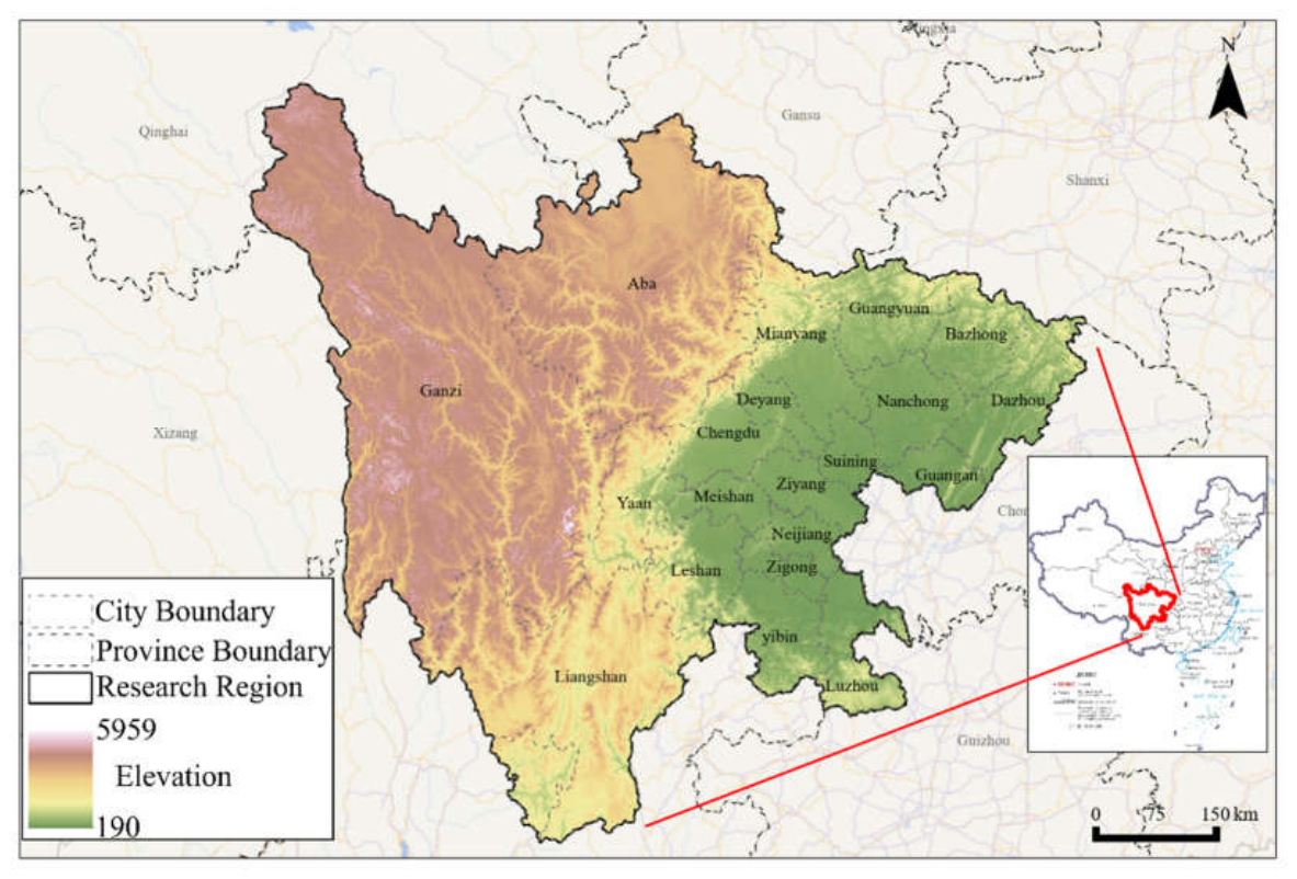
Sichuan Province (28°N–34°N, 97°E–109°E) is located in inland southwestern China, with a total area of 486,000 km2. In 2023, its permanent population was 83.68 million, and the urbanization rate reached 59.1% (Sichuan Provincial Bureau of Statistics, 2024). As the only Chinese province covering the Qinghai-Tibet Plateau, Hengduan Mountains, and Sichuan Basin, it shows a clear west–ecology, east–economy pattern. The western plateau and mountainous area (48.1% of the province, average elevation >3,000 m) contains 87% of ecological redline zones. The eastern basin and hills (51.9% of the area) hold 78% of cropland and 92% of urban construction land (Sichuan Provincial Department of Natural Resources, 2023). This strong spatial heterogeneity makes Sichuan an ideal case for studying territorial spatial functional conflicts, supporting grid analysis, coupling coordination, and carbon emission–economy research.
Figure 1.
Overview Map of the Sichuan Province.
2.2. Data Sources
The data used in this study include raster data, vector data, and statistical data. Data sources are presented in Table 1. Specifically: 1) Raster data mainly include land change survey data and GDP data for Sichuan Province. 2) Vector data primarily comprise the administrative boundary of Sichuan Province. 3) Statistical data mainly cover fossil energy consumption, forest fire area, crop yield, coal mining output, oil and natural gas production, industrial product output, livestock inventory, population size, rice planting area, domestic waste landfill volume, domestic waste incineration volume, and COD emissions. These statistical data are used to calculate the net carbon emissions of Sichuan Province. To meet the requirements of subsequent analyses, all data were preprocessed using the ESRI ArcGIS platform: 1) Coordinate system unification: All data were converted to a consistent coordinate reference system, with the geographic coordinate system set to WGS-1984 and the projected coordinate system based on a customized Albers projection (first standard parallel: 25°, second standard parallel: 47°, central meridian: 105°). 2) Data resampling: Using Python-based data processing tools, the GDP, net carbon emissions, and functional classification raster data were resampled to an image size of 1035 × 934 pixels.
2.3. Methods
2.3.1. Analysis of Territorial Spatial Functional Conflicts
- Classification of Territorial Spatial Functions
This study constructs a territorial spatial function classification system based on land use types, following the principles of “function dominance, multi-level classification, and dynamic adaptation”. Drawing on relevant research findings[34] and the technical specifications of the Guidelines for Land and Sea Space Classification for Territorial Spatial Survey, Planning, and Use Control (Ministry of Natural Resources, 2023), a classification framework is established(Table 2).
Classification framework construction: Primary and secondary classes are divided based on dominant functions, highlighting the “core responsibilities” of spatial use (e.g., ecological space with carbon sequestration and biodiversity maintenance as its primary functions). Tertiary classes are refined according to the Current Land Use Classification (GB/T 21010-2017), for example, subdividing “urban production space” into industrial land, logistics and warehousing land, etc.
Functional classification basis: Following the Guidelines for Land and Sea Space Classification for Territorial Spatial Survey, Planning, and Use Control (Ministry of Natural Resources of the People’s Republic of China, 2023) and prioritizing the functional attributes of land use types, this study integrates the “Production-Living-Ecological Space” (PLE Space) theory and the “Three Zones and Three Lines” (urban, agricultural, and ecological zones along with their corresponding control lines) management requirements. Consequently, the territorial spatial functions are classified into five secondary categories: urban production space, urban living space, rural production space, rural living space, and ecological space.
Land use classification basis: The study period spans the Second National Land Survey and the Third National Land Survey. To maintain consistency in land use classification, this study adopts the official classification document from the Second National Land Survey, i.e., the Current Land Use Classification (GB/T 21010-2007). A total of 37 land use types are classified at the tertiary level, including: mining land, port and wharf land, highway land, pipeline transport land, airport land, railway land, urban land, town land, paddy fields, dry land, irrigated land, ridge land, canals, tea gardens, orchards, rural roads, other orchard land, agricultural facility land, village land, hydraulic structure land, glaciers and permanent snow, scenic and special land, shrubland, river surfaces, lake surfaces, pond surfaces, bare land, inland mudflats, other grassland, other forestland, artificial pastureland, sandy land, reservoir surfaces, natural pastureland, saline-alkali land, forestland, and marshland.
Land use type to functional space mapping: Based on the “land use–territorial spatial function” correspondence database established in previous research and referring to the spatial mapping standards of similar classification studies, this study integrated expert consultation opinions to merge the land use types of Sichuan Province into the five functional spaces. The classification results are presented in Supplementary Method S1[3,35,36,37,38,39].
- 2.
- Calculation of the TSFC Index
Based on the territorial spatial function classification data, this study constructs a territorial spatial functional conflict assessment index derived from landscape ecological risk assessment theory and landscape ecology principles[40,41]. It should be clarified that this study does not equate landscape ecological risk directly with territorial spatial functional conflicts. Instead, we take the landscape ecological risk index as a pattern-based proxy indicator to quantify the intensity of TSFCs, grounded in the inherent correspondence between landscape pattern features and functional conflict processes.
The theoretical rationale for this mapping is established in three dimensions:
(1) Landscape complexity - functional competition intensity. The complexity of adjacent landscape patches reflects the degree of spatial interleaving among different territorial spatial functions (production, living, ecological). Higher landscape complexity indicates more frequent functional interactions and more intense competition for spatial resources, which is the core manifestation of TSFCs[42].
(2) Landscape vulnerability - conflict potential risk. Different functional spaces differ significantly in resistance to external disturbance. Ecological spaces with high vulnerability are more likely to be squeezed by production and living spaces, thus bearing higher potential conflict risk. This dimension captures the asymmetry of functional conflict impacts[43,44].
(3) Landscape fragmentation - conflict spatial dispersion. Fragmented landscape patterns correspond to scattered spatial allocation of various functions, which reduces the stability of the territorial spatial function system and intensifies the incoordination of development behaviors among different stakeholders, further aggravating functional conflicts[19,21].
Following this analytical framework, we characterize risk sources with landscape complexity indices, risk receptors with ecological vulnerability indices, and risk effects with landscape fragmentation indices (Figure 2). The composite index synthesized from the three dimensions is defined as the Territorial Spatial Functional Conflict Index (TSFCI), which quantifies the relative intensity of functional conflicts from the landscape pattern perspective. The detailed calculation workflow is provided in Supplementary Method S2.
- 3.
- Analysis of Spatiotemporal Distribution Characteristics of TSFCs
To facilitate the identification of TSFCs intensity across different regions, this study classifies the TSFCI calculated at the county scale. Although spatial indices are commonly classified using the natural breaks (Jenks) method or the quantile method[42], this study adopts the equal interval method to enhance cross-year comparability and improve the interpretability of TSFCI. Specifically, the TSFCI is divided into 10 classes by equally partitioning the range from its minimum to maximum value into 10 intervals, with each interval corresponding to a conflict level (levels 1 to 10, Table 3).
2.3.2. Analysis of Economic-Environmental Coupling Synergy
In this study, two methods are employed to characterize the synergy between economic growth and carbon emission in territorial space. First, the CCD model is used to calculate the coupling coordination degree between economic benefits and carbon emissions for each spatial unit, thereby obtaining the spatial distribution of the CCD between economic growth and carbon emissions. Second, the Tapio decoupling model is applied to calculate the decoupling elasticity index(DEI) between economic benefits and carbon emissions for each spatial unit, revealing the correlation between economic growth and carbon emission. By integrating the CCD and the DEI, this study comprehensively characterizes the spatiotemporal patterns of the synergy between economic growth and carbon emission in territorial space.
- Calculation of Net Carbon Emission
Based on the “2006 IPCC Guidelines for National Greenhouse Gas Inventories”, the “2019 Refinement, the Provincial Greenhouse Gas Inventory Compilation Guidelines (Trial)”, and relevant domestic and international studies, and taking into account the actual situation of Sichuan Province, this study integrates carbon source and carbon sink accounting items to construct a territorial carbon source and carbon sink inventory for Sichuan Province (Table 4). This study adopts a territorial production-based accounting framework, that is, all carbon emissions and sinks generated within the geographical scope of Sichuan Province are included in the accounting, regardless of whether the corresponding products and services are consumed locally or outside the province. This accounting principle is consistent with the official greenhouse gas inventory compilation specifications and most regional carbon emission studies, ensuring the comparability of results. The carbon source inventory comprises four sectors (energy sector; industrial processes and product use sector; agriculture, forestry, and other land use sector; and waste sector) and 11 categories: carbon emissions from fossil fuel combustion, forest fires, straw burning, coal mining fugitive emissions, oil and natural gas system fugitive emissions, industrial processes, livestock enteric fermentation and manure management, animal respiration, rice cultivation, solid waste treatment, and wastewater treatment. The carbon sink inventory refers to carbon sink by terrestrial ecosystems.
It should be further noted that, based on relevant research findings and considerations of accounting feasibility, this study does not include carbon sink by cropland vegetation, constructed land, or unused land in the accounting scope. Instead, only carbon sink by forestland (shrubland, forestland, and other forestland), grassland (natural pastureland, artificial pastureland, and other grassland), and water bodies (lake surfaces, pond surfaces, reservoir surfaces, marshland, river surfaces, inland mudflats, and hydraulic structure land) is considered. The rationale is as follows: although crops possess some carbon sink capacity during their growth cycle, their relatively short growth period, combined with the fact that most of the biomass is released back into the atmosphere through decomposition or utilization after harvest, makes it difficult to achieve long-term stable carbon sequestration[45]. Meanwhile, constructed land is predominantly characterized by carbon emissions, and the carbon sink of unused land is generally small, resulting in a limited contribution of both to regional carbon sink.
Following the carbon emission calculation methods and basic parameters proposed by the IPCC and related studies (see Supplementary Method S3), the carbon emissions and carbon sink for each accounting item in Sichuan Province from 2010 to 2022 were calculated. The carbon emissions and carbon sink were then spatially downscaled using the following methods: (1) Carbon emissions from fossil fuel combustion were spatially allocated based on the spatial weights of nighttime light data for Sichuan Province. (2) Carbon emissions from human respiration, solid waste treatment, and domestic wastewater treatment were spatially allocated based on the spatial weights of population density data for Sichuan Province. (3) Carbon emissions from forest fires were distributed equally across all forestland spatial units. (4) Carbon emissions from straw burning and rice cultivation were distributed equally across all cropland spatial units; carbon emissions from coal mining fugitive emissions, oil and natural gas system fugitive emissions, industrial processes, and industrial wastewater treatment were distributed equally across all industrial and mining land spatial units. (5) Carbon emissions from livestock enteric fermentation and manure management, as well as from livestock respiration, were distributed equally across all grassland spatial units. (6) Carbon sink by forestland, grassland, and water bodies was distributed equally across forestland, grassland, and water body spatial units, respectively.
It should be specifically noted that forestland (shrubland, forestland, and other forestland), cropland (dry land, irrigated land, and paddy fields), and grassland (natural pastureland, artificial pastureland, and other grassland) are represented as raster data with a resolution of 120 m × 120 m, while industrial and mining land and water bodies (lake surfaces, pond surfaces, reservoir surfaces, marshland, river surfaces, inland mudflats, and hydraulic structure land) are represented as raster data with a resolution of 15 m × 15 m. When allocating carbon emissions equally using land use data, the land use raster data at 120 m × 120 m and 15 m × 15 m resolutions were first resampled to 125 m × 125 m and 25 m × 25 m resolutions, respectively. Carbon emissions were then allocated equally to the spatial grids corresponding to each land use type. Finally, a 250 m × 250 m vector grid for Sichuan Province was used to aggregate and compile the carbon emission data within each grid cell, producing spatial distribution maps of carbon emissions and carbon sink for Sichuan Province from 2010 to 2022. On this basis, the spatial distribution map of net carbon emissions for Sichuan Province from 2010 to 2022 was generated using the Raster Calculator tool in the ESRI ArcGIS platform. The net carbon emission results for Sichuan Province are presented in Supplementary Method S3.
- 2.
- Calculation of the CCD
By calculating the CCD between economic benefits and carbon emissions for each spatial unit, the spatial distribution of the CCD between economic growth and carbon emission is obtained, characterizing the spatial features of the synergy between economic growth and carbon emission in territorial space. The coupling coordination degree for each spatial unit is calculated using the following formulas:
where represents the coupling degree; and denote the normalized economic benefits and carbon emissions of the -th spatial unit, respectively; is the comprehensive coordination index of economic benefits and carbon emissions, representing the overall influence of the performance levels of the economic system and the carbon emission system on the CCD; and represents the CCD between economic growth and carbon emission.

Table 5.
Coupling Coordination between Economic Growth and Carbon Emission Reduction.
| Value of D | Class | Development stages |
|---|---|---|
| 0.0 ≤ D < 0.25 | 1 | Seriously unbalanced |
| 0.25 ≤ D < 0.5 | 2 | Slightly unbalanced |
| 0.5 ≤ D < 0.75 | 3 | Barely balanced |
| 0.75 ≤ D < 1.0 | 4 | With superior balance |
The CCD model was applied to calculate the coupling coordination degree between GDP and net carbon emissions for each spatial grid at five time points (2010, 2013, 2016, 2019, and 2022). The spatial distribution of the CCD between economic growth and carbon emission in Sichuan Province was then obtained, and its spatial distribution characteristics were analyzed.
- 3.
- Calculation of the Decoupling Elasticity Index
The Tapio decoupling model[24] is one of the most commonly used models in decoupling analysis, and this study adopts it for analysis. Research has shown that the Tapio decoupling model is more robust than the OECD decoupling elasticity index model. For instance, the original OECD decoupling method has a limitation in its sensitivity to the choice of base period, which leads to unstable calculation results. Moreover, this method lacks clear judgment criteria, making it prone to measurement errors[46]. In contrast, Tapio’s decoupling analysis provides stable results that are not affected by changes in statistical dimensions, thereby better reflecting the decoupling state between economic development and carbon emissions.
According to Tapio’s definition, the decoupling elasticity index equation is calculated as follows:
Where, is the decoupling elasticity index, which measures the degree of decoupling between economic growth and carbon emissions.and denote the carbon dioxide emissions in the study year and the base year, respectively, while and denote the corresponding GDP values (at constant prices). The terms and represent the changes in carbon emissions and GDP, respectively, between the study period and the base period. Drawing on the decoupling elasticity index framework established by Tapio[24], eight distinct decoupling types are defined and summarized in Table 6 .
2.3.3. Association Between TSFCs and the Synergy Between Economic Benefits and Net Carbon Emissions
Economic conditions, carbon emissions, and TSFs exhibit evident spatiotemporal heterogeneity; however, the spatial interactions between TSFC and economic growth, carbon emission reduction, and their synergy remain unconfirmed, introducing uncertainty into coordinated governance efforts. This study employs the single-factor geographical detector, phased geographical detector, and Mann-Kendall trend test to conduct systematic analysis from both spatial and temporal perspectives.
- Spatial Association of TSFCs and the Synergy Between Economic Benefits and Net Carbon Emissions
This study applies the GD model to quantitatively measure the spatiotemporal coupling between TSFCs, GDP, and net carbon emissions, in order to explore the statistical linkage between TSFC patterns and the economic-environmental synergy. The model measures the explanatory power of independent variables regarding the spatial differentiation of dependent variables based on the principle of variance decomposition. This power is expressed as the q-statistic, and is calculated as follows:
Where indexes the category of territorial spatial functions, with ; and represent the total number of territorial spatial function patches and the number of patches belonging to category , respectively; denotes the variance of economic benefits, carbon emissions, or their coupling coordination degree—calculated both across all patches and within the patches of category ; and quantifies the explanatory power between the spatial distribution of territorial spatial functions and that of economic benefits, carbon emissions, or their CCD.
The TSFCI is a continuous index ranging from 0 to 1. To meet the input requirement of the geographical detector model (independent variables must be categorical), we adopted the equal interval method consistent with the TSFCI grading system in Table 3 to discretize the index, which ensures consistency with the conflict intensity classification framework used throughout the study. Initially, the index was divided into 10 equal-interval levels (levels 1–10). Considering that levels 1, 2, and 10 had extremely small sample sizes which would lead to unstable variance estimation within strata, we merged these low-sample levels into adjacent categories, resulting in 7 final categories (levels 3–9) for model input. This setting balances grading granularity and statistical reliability of each stratum.
Empirically, Sichuan Province was partitioned into 183 county-level administrative units. For each unit, the mean and median values of the TSFCI, the economic-environmental coupling coordination degree, and the economic-environmental DEI were computed. These aggregated values were subsequently linked to the county-level vector layer. A geographical detector analysis was then carried out, yielding statistical results at the county scale.
- 2.
- Temporal Association Between TSFCs and the Synergy Between Economic Growth and carbon emission
To further reveal the temporal evolution characteristics of the association between TSFCs and the economic-environmental synergy, this study conducts time-stratified geographical detector analysis and Mann-Kendall non-parametric trend testing based on the spatial geographical detector analysis.
The study period 2010–2022 is divided into four consecutive periods (2010–2013, 2013–2016, 2016–2019, and 2019–2022). For each period, a single-factor geographical detector model is constructed using the TSFCI at the beginning of the period as the independent variable and the DEI of the corresponding period as the dependent variable, to compare the temporal changes in q-statistics and identify the temporal evolution of the explanatory power. Additionally, a year-by-year geographical detector analysis is conducted using the TSFCI for the years 2010, 2013, 2016, 2019, and 2022 as independent variables and the CCD of the corresponding years as dependent variables, to supplementarily verify the temporal stability of the explanatory power. Non-parametric trend tests are performed on the time series of q-statistics, median TSFCI, median CCD, and median DEI to determine whether there is a significant linear upward or downward trend, with the Theil-Sen median slope estimator used to quantify the magnitude of change.
3. Results
3.1. Spatiotemporal Characteristics of TSFCs
To enhance regional readability, the TSFCI calculated at the county scale was aggregated and visualized at the prefectural (city) level. Subsequent geographical detector analyses, however, retained the 183 county-level administrative units as the basic analytical sample. Using the TSFCI constructed from landscape pattern indices, this study measured the intensity of TSFCs for each prefecture-level city in Sichuan Province from 2010 to 2022(Appendix A Table A1). The results indicate that TSFCs in Sichuan Province exhibit pronounced spatiotemporal heterogeneity, with clear regional differentiation and phased evolutionary trends (Figure 3).
At the overall level, the TSFCI for most prefecture-level cities falls within the range of 0.6–0.8, corresponding to a moderately high conflict level. From 2010 to 2016, the average TSFCI values across cities remained relatively stable, with most regions maintaining TSFCI averages between 0.68 and 0.76, indicating a persistently strong competitive relationship among different territorial spatial functions during the period of rapid industrialization and urbanization.
From a temporal perspective, the TSFCI in most regions exhibited minor fluctuations from 2010 to 2016, generally remaining stable. For instance, Nanchong, Yibin, Bazhong, Zigong, and Suining maintained TSFCI averages above 0.73 over an extended period, indicating persistent high-intensity competition in territorial spatial development and utilization.
However, a clear trend of differentiation in TSFCs emerged after 2016. On the one hand, conflict intensity markedly decreased in some traditional resource development and mountainous regions. For example, the mean TSFCI in Liangshan Prefecture decreased from 0.619 in 2010 to 0.435 in 2022, in Ganzi Prefecture from 0.555 to 0.307, in Aba Prefecture from 0.561 to 0.314, and in Yaan City from 0.604 to 0.398. This indicates that, driven by ecological protection policies, the “Three Lines One Permit” (TLOP), and ecological restoration projects, TSFCs have been alleviated in the western Sichuan Plateau and ecologically dominant areas. On the other hand, conflict intensity has steadily increased in parts of the Chengdu-Chongqing Economic Circle and urbanized areas in eastern Sichuan. For instance, the mean TSFCI in Ziyang City increased from 0.709 in 2010 to 0.815 in 2022, in Neijiang City from 0.727 to 0.802, in Zigong City from 0.749 to 0.802, and in Guangan City from 0.685 to 0.741, suggesting that rapid urban expansion, transportation infrastructure construction, and industrial agglomeration have substantially intensified the competitive relationship between production and ecological spaces.
Furthermore, to further reveal the dynamic evolutionary characteristics of TSFCs across different regional types, this study selected Luzhou, Nanchong, Liangshan, Aba, and Chengdu as representative examples from the southeast, northeast, southwest, northwest, and central regions, respectively, based on spatial location and development characteristics of Sichuan Province. The trends in TSFCI from 2010 to 2022 were then analyzed (Figure 4).
The results reveal significant regional disparities in the evolution of TSFC across Sichuan Province. Overall, basin and highly urbanized regions such as Chengdu, Nanchong, and Luzhou maintain persistently high conflict levels, while ecology-dominated areas like Aba and Liangshan exhibit relatively low values.Chengdu shows consistently high TSFC (0.67–0.70), driven by intense population agglomeration and urban expansion, with ongoing ecological restoration unable to fully offset development pressure. Nanchong maintains stable, high TSFC (>0.74) due to combined agricultural and urban expansion. Luzhou’s TSFC declined from 0.73 to 0.61, indicating moderate conflict alleviation, though spatial heterogeneity increased.Western ecological regions display distinct trends: TSFC remained low and decreased notably after 2016, from 0.56 to 0.31 in Aba and from 0.62 to 0.44 in Liangshan, reflecting effective ecological protection policies.Spatially, TSFC exhibits an east intensification–west mitigation pattern, with high conflict in economically active areas and low conflict in ecological zones. Population density, industrial structure, development intensity, and ecological policies are key drivers of TSFC spatiotemporal variation.
In summary, TSFCs in Sichuan Province from 2010 to 2022 exhibited pronounced regional differentiation and phased evolutionary characteristics. Conflicts in ecologically dominant areas tended to alleviate, while those in rapidly urbanizing and industrializing regions continued to intensify, indicating a substantial correlation between TSFCs and the intensity of regional economic development, population agglomeration, and ecological protection policies.
3.2. Spatiotemporal Characteristics of the Synergy Between Economic Benefits and Net Carbon Emissions
To comprehensively characterize this synergy, this study employs both the CCD model and the Tapio decoupling model. The CCD reflects the coordinated development level between the economic and carbon emission systems, while the DEI measures the response relationship between economic growth and carbon emission changes, identifying whether growth has shed its reliance on emission increases. Their combination reveals both the overall coordination of the economic-environmental system and its dynamic correlation, offering a more comprehensive characterization of the spatiotemporal evolution of the synergy between economic growth and carbon emission in Sichuan Province.
The results indicate that from 2010 to 2022, the synergy between economic growth and carbon emission in Sichuan Province exhibited pronounced spatiotemporal heterogeneity and phased evolution, with substantial differences in CCD levels and decoupling states across regions, and a substantial spatial correlation with the pattern of TSFCs.
3.2.1. Spatiotemporal Characteristics of the CCD
Based on the CCD model, the synergy between GDP and net carbon emissions in Sichuan Province from 2010 to 2022 was measured. The results indicate that the overall coordination between economic growth and carbon emission in Sichuan Province remains at a relatively low level, yet exhibits pronounced spatial heterogeneity and regional differentiation. During the study period, CCD values for most prefecture-level cities were mainly concentrated between 0.20 and 0.40, generally falling within the “severe disorder to mild disorder” range, suggesting that a stable coordinated relationship between economic growth and net carbon emissions has not yet been established in Sichuan Province (Figure 5).
From a temporal perspective, CCDs in most prefecture-level cities exhibited only minor fluctuations from 2010 to 2022, generally showing a slight downward trend. For example, the mean CCD in Chengdu decreased from 0.403 in 2010 to 0.395 in 2022, in Deyang from 0.347 to 0.340, in Neijiang from 0.283 to 0.278, and in Nanchong from 0.267 to 0.262. Overall, although Sichuan’s total economic output continued to grow during the study period, the simultaneous increase in carbon reduction pressure led to stagnation in the coordination level between economic growth and carbon emission (Appendix B Table A2).
From the perspective of spatial heterogeneity, CCDs in Sichuan Province generally present a pattern of “higher in the Chengdu Plain, lower in the western Sichuan ecological zone.” Chengdu maintains the highest coordination level in the province over the long term, with its mean CCD stabilizing between 0.39 and 0.41—substantially higher than other cities. This indicates that Chengdu, as the province’s core economic region, possesses substantial advantages in industrial structure optimization, green technology investment, and energy efficiency, resulting in a relatively high synergy capacity between economic growth and carbon emission. Deyang and Neijiang, which have relatively high degrees of industrialization, also exhibit higher coordination levels, suggesting that industrial agglomeration and technological progress have promoted the coordinated development of the economic-environmental system to some extent.
In contrast, CCDs in ecologically dominant regions of western Sichuan, such as Aba and Liangshan, have remained persistently low. The mean CCD in Aba decreased from 0.234 in 2010 to 0.229 in 2022, and in Liangshan from 0.240 to 0.235, generally remaining in the “moderate disorder” stage. This indicates that in regions with strong ecological protection constraints and relatively weak economic foundations, although carbon emission levels are low, insufficient economic development capacity makes it difficult to achieve effective synergy between economic growth and carbon emission.
For further analysis, Chengdu, Aba, Liangshan, Nanchong and Luzhou were selected as typical cities and prefectures, and the relevant results are presented in Supplementary Results S4.
In summary, from 2010 to 2022, the CCD between economic growth and carbon emission in Sichuan Province remained at a relatively low level, yet with substantial spatial heterogeneity across regions. The economic core region exhibited a relatively strong coordination capacity, while ecologically dominant areas and traditional resource-dependent regions showed relatively low coordination levels. This indicates that regional economic foundation, industrial structure, energy efficiency, and ecological protection constraints are important factors influencing the synergy between economic growth and carbon emission in Sichuan Province. Furthermore, the spatial pattern of CCD exhibits a certain correspondence with the spatial pattern of TSFCs. However, this relationship is not a simple linear decline but rather manifests as hierarchical differences in the economic-environmental synergy state across different conflict levels. Regions with moderate conflict levels may possess a higher capacity to balance development and protection, whereas regions with high conflict levels are more prone to accumulating structural contradictions between economic growth and carbon emission.
3.2.2. Spatiotemporal Characteristics of the DEI
Based on the dynamic relationship between GDP and net carbon emissions in Sichuan Province from 2010 to 2022, as measured by the Tapio decoupling model (for detailed DEI data, see Supplementary Table S5), the results indicate that there are certain decoupling characteristics between economic growth and net carbon emissions in Sichuan Province. However, this decoupling is not a continuous and stable unidirectional improvement process; rather, it exhibits pronounced characteristics of phased fluctuations and structural transformation (Figure 6).
From the perspective of the overall structure, strong decoupling(SD), weak decoupling (WD), and recessive decoupling(RD) are the main decoupling types in Sichuan Province during the study period. From 2010 to 2013, SD accounted for 53.4%, while WD and RD accounted for 4.3% and 42.3%, respectively. From 2013 to 2016, SD remained dominant with a proportion of 52.7%, but the proportion of WD increased significantly to 39.4%. This indicates that although some regions achieved economic growth faster than carbon emission growth, the pressure of rising carbon emissions still persisted. From 2016 to 2019, the proportion of SD further increased to 60.8%—the highest level during the study period—while the proportion of RD was 32.3%. This indicates that the dependence of carbon emissions on economic growth weakened to some extent, and the coordination between economic growth and carbon emission was relatively favorable.
From 2019 to 2022, the decoupling structure in Sichuan Province underwent pronounced changes. The proportion of SD decreased to 34.7%, while the proportion of RD rose to 52.0%, becoming the dominant decoupling type during this stage. This suggests that the decline in carbon emissions in some regions during the later period may have been accompanied by economic slowdown or contraction of economic activities, rather than being equivalent to stable green growth-oriented decoupling. Therefore, the period from 2019 to 2022 should be understood as a stage dominated by RD, reflecting that the synergy between economic growth and carbon emission in Sichuan Province remains volatile, and the stability and quality of the low-carbon transition still need improvement. Overall, Sichuan Province exhibited relatively positive changes dominated by SD from 2010 to 2019, but shifted to RD from 2019 to 2022. his indicates that the relationship between economic growth and carbon emission is characterized by phased changes rather than a continuously optimizing linear process.
Table 7.
Proportion of decoupling types in Sichuan Province.
| Period | SD | WD | RD | SND | WND | END | EC | RC |
|---|---|---|---|---|---|---|---|---|
| 2010-2013 | 53.38 | 4.32 | 42.30 | 0 | 0 | 0 | 0 | 0 |
| 2013-2016 | 52.72 | 39.37 | 3.74 | 0 | 2.40 | 1.78 | 0 | 0 |
| 2016-2019 | 60.75 | 6.98 | 32.28 | 0 | 0 | 0 | 0 | 0 |
| 2019-2022 | 34.72 | 13.30 | 51.98 | 0 | 0 | 0 | 0 | 0 |
Note: SD: Strong decoupling, WD: Weak decoupling, RD: Recessive decoupling, SND: Strong negative decoupling, WND: Weak negative decoupling, END: Expansive negative decoupling, EC: Expansive coupling, RC: Recessive coupling.
From the perspective of spatial heterogeneity (Supplementary Table S5 for detailed data), the decoupling state in Sichuan Province exhibits certain regional differentiation, roughly manifested as the following spatial characteristics: relatively prominent growth-oriented decoupling in the Chengdu Plain Economic Zone, pronounced stage fluctuations in the industrialized areas of southern Sichuan, and relatively distinctive decoupling types in the ecological function zones of western Sichuan.
To explore the evolutionary patterns of decoupling between economic growth and net carbon emissions across different regions in Sichuan Province, this study selects Chengdu, Nanchong, Luzhou, Liangshan, and Aba for comparative analysis(Figure 7). The results show significant regional disparities in decoupling characteristics: Chengdu is dominated by growth-oriented decoupling with the optimal decoupling level; Nanchong and Luzhou maintain stable decoupling states but see slow progress in low-carbon transformation. Aba and Liangshan follow development paths distinctly different from those of basin cities. Due to low regional development intensity and strong ecological protection constraints, the two regions exhibit alternating characteristics of strong decoupling (SD), weak decoupling (WD), and recessive decoupling (RD) across different periods. Among these, strong decoupling indicates that economic growth and net carbon emission reduction can occur simultaneously in certain stages. However, considering the small industrial scale and low carbon emission base in the western Sichuan Plateau ecological function zone, their strong decoupling does not fully equate to proactive decoupling driven by industrial green upgrading. In contrast, periods with a high proportion of recessive decoupling largely reflect passive emission reduction under conditions of low economic activity intensity or slowing economic growth. This suggests that although the western Sichuan ecological function zone faces relatively low pressure from carbon emission growth, its decoupling state exhibits obvious eco-constrained attributes.
In summary, a decoupling trend between economic growth and carbon emission preliminarily emerged in Sichuan Province from 2010 to 2022. Nevertheless, the mechanisms underlying decoupling differ considerably across regions. In economic core areas such as Chengdu, decoupling may primarily reflect growth-oriented decoupling driven by industrial structure optimization, energy utilization efficiency improvement, and green technology application. In ecological function zones such as Aba and Liangshan, decoupling is more influenced by a combination of low development intensity, ecological protection constraints, and a low carbon emission base. In traditional industrial or agricultural–industrial composite regions such as Nanchong and Luzhou, economic growth has not yet fully shed its dependence on resource consumption and carbon emissions.
These findings reveal significant spatial heterogeneity in the synergy between economic growth and carbon emission across Sichuan Province. Furthermore, this heterogeneity is likely associated with the spatial pattern of TSFCs identified earlier, providing a foundation for further analysis of the association between TSFCs and the synergy between economic growth and carbon emission.
3.3. Association Between TSFCs and the Synergy Between Economic Benefits and Net Carbon Emissions
3.3.1. Spatial Association Between TSFCs and the Synergy Between Economic Benefits and Net Carbon Emissions
To identify the explanatory role of TSFCs in the spatial heterogeneity of the synergistic state between economic growth and carbon emission, this study takes the 183 county-level administrative units in Sichuan Province as the basic analytical units and constructs a single-factor geographical detector model for the entire region. The independent variable X is defined as the median level of TSFCI at the county level, while the dependent variables Y are the median values of the CCD and the DEI between carbon emissions and GDP, respectively. The CCD is a static indicator measured at five time points (2010, 2013, 2016, 2019, and 2022), yielding 915 valid samples (5 years × 183 counties) for the CCD model. The DEI is a dynamic indicator measuring changes between adjacent years, corresponding to four periods (2010–2013, 2013–2016, 2016–2019, and 2019–2022), thus yielding 732 valid samples (4 periods × 183 counties) for the DEI model. By comparing the within-group and between-group variances of CCD and DEI across different TSFCI levels, it is possible to determine whether TSFCI levels can explain the spatial heterogeneity of the synergistic state between economic growth and carbon emission.
Table 8.
Results of the single-factor geographical detector analysis for CCD and DEI.
| Analysis dimension | Dependent variable | samples | X categories | q-statistic | F-statistic | p-value | Significance |
| Static coupling coordination | Median CCD | 915 | 7 | 0.081 | 15.52 | p<0.001 | *** |
| Dynamic decoupling process | Median DEI | 732 | 7 | 0.023 | 4.33 | p<0.001 | *** |
Note:*** denotes extremely significant, ** denotes very significant, * denotes significant.
The single-factor geographical detector analysis reveals that the median TSFCI level exerts a significant explanatory effect on the spatial heterogeneity of both CCD and DEI. For CCD, the q-statistic is 0.081, indicating that approximately 8.1% of the spatial variation in the county-level coupling coordination degree across Sichuan Province can be attributed to TSFCI levels. For DEI, the q-statistic is 0.023, suggesting that about 2.30% of its spatial variation is explained by TSFCI levels. With both models yielding p-values below 0.001, these results establish a stable statistical association between TSFCs and the synergy between economic growth and carbon emission. Nevertheless, judging from the magnitude of the q-statistics, the explanatory power of TSFCI for both CCD and DEI is not substantial, with its full-period explanatory power for DEI being particularly weak. Consequently, TSFCs should be interpreted as one of the significant factors influencing the spatial heterogeneity of the synergy between economic growth and carbon emission, rather than the exclusive or decisive determinant.
Figure 8.
Explanatory power of TSFC for CCD and DEI based on the geographical detector model.
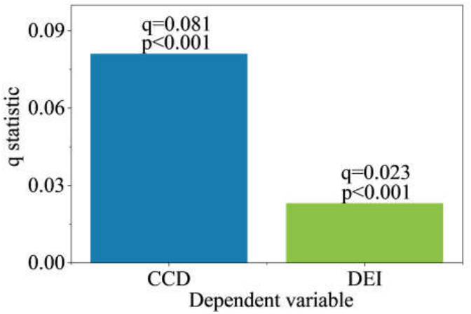
A further comparison between the CCD and DEI models reveals that the explanatory power of TSFCI for CCD is substantially higher than that for DEI. This indicates that, in the full-period pooled analysis, the explanatory role of TSFCs in the spatial heterogeneity of static coupling coordination levels is stronger than their overall explanatory role in the dynamic decoupling process. This discrepancy may be attributed to the following: CCD represents the comprehensive coordination status between the economic system and the carbon emission system at a given point in time, characterized by strong spatial stability. By contrast, DEI represents the dynamic relationship between economic growth and changes in carbon emissions over consecutive periods, rendering it more sensitive to episodic economic fluctuations, emission variations, industrial restructuring, and exogenous shocks. Therefore, while DEI may demonstrate considerable explanatory power in period-by-period analyses, the overall explanatory power of TSFCI for its spatial heterogeneity is inevitably diluted by inter-period volatility when the data are pooled across the full study period.
An examination of the stratified DEI statistics across TSFCI levels reveals that the influence of TSFCs on the dynamic decoupling state is not linear. According to the full-period pooled results, the mean DEI is highest for TSFCI level 6 (0.767), followed by level 8 (0.267), whereas levels 5 and 7 yield considerably lower means (-1.148 and -0.018, respectively). These findings preclude any simple linear inference—such as “greater conflict intensity leads to a poorer decoupling state” or “greater conflict intensity leads to a better decoupling state.” On the contrary, the effect of TSFCI on DEI exhibits pronounced hierarchical variation and phase-dependent sensitivity. Moderate-conflict regions, characterized by a combination of moderate development intensity and ecological constraints, may achieve relatively high decoupling levels during certain periods. Meanwhile, high-conflict or low-conflict regions display substantial internal heterogeneity, with their decoupling states additionally modulated by industrial structure, economic foundations, energy consumption patterns, and carbon sink conditions. Consequently, the discussion that follows should emphasize the nonlinear characteristics of their statistical association with TSFCs, rather than interpreting it as a unidirectional, linear driving mechanism.
Table 9.
CCD、DEI summary by TSFC level.
| TSFC level | indicator | count | mean | std |
|---|---|---|---|---|
| 3 | CCD |
72 | 0.223 | 0.003 |
| 4 | 23 | 0.333 | 0.246 | |
| 5 | 21 | 0.433 | 0.305 | |
| 6 | 135 | 0.260 | 0.131 | |
| 7 | 201 | 0.328 | 0.191 | |
| 8 | 402 | 0.257 | 0.080 | |
| 9 | 61 | 0.243 | 0.039 | |
| 3 | DEI |
37 | 0.197 | 0.005 |
| 4 | 12 | -0.130 | 1.224 | |
| 5 | 12 | -1.150 | 3.501 | |
| 6 | 113 | 0.767 | 2.852 | |
| 7 | 180 | -0.020 | 1.555 | |
| 8 | 344 | 0.267 | 1.092 | |
| 9 | 34 | 0.153 | 0.542 |
To verify the sensitivity of the results to discretization schemes, we conducted two sets of robustness tests: (1) varying the number of categories (5, 7, and 9 equal-interval levels); (2) applying different classification methods (equal interval, natural breaks, and quantile, all with 7 categories). The results show that across all schemes, TSFCI always has significant explanatory power for both CCD and DEI (p < 0.001), and the relative magnitude of q-values remains stable, with only small fluctuations in absolute values. This indicates that the core conclusion of a significant statistical association between TSFCs and economic-carbon synergy is robust to discretization settings.
3.3.2. Temporal Association Between TSFCs and the Synergy Between Economic Growth and Carbon Emission
To further reveal the temporal evolution characteristics of the Association Between TSFCs and the synergy between economic growth and carbon emission, this study conducts time-stratified geographical detector analysis and Mann-Kendall trend testing based on the full-region single-factor geographical detector analysis. Specifically, for the dynamic decoupling process, the median DEI values for four consecutive periods (2010–2013, 2013–2016, 2016–2019, and 2019–2022) are used as dependent variables, and the median TSFCI level at the beginning of each period is used as the independent variable to construct period-specific single-factor geographical detector models. For the static coupling coordination state, the median CCD values for the years 2010, 2013, 2016, 2019, and 2022 are used as dependent variables, and the median TSFCI level for the corresponding year is used as the independent variable to construct year-specific single-factor geographical detector models. On this basis, Mann-Kendall non-parametric trend tests are performed on the period-specific q-values for DEI, the year-specific q-values for CCD, and the temporal series of TSFCI, CCD, and DEI to determine whether there are significant unidirectional trends.
The time-stratified geographical detector results for DEI demonstrate that the explanatory power of TSFCI for the dynamic decoupling relationship between economic growth and carbon emissions exhibits pronounced temporal fluctuations. During 2010–2013, the explanatory power of TSFCI for DEI reached its peak, with a q-value of 0.254, indicating that TSFCI levels accounted for 25.4% of the spatial variation in county-level DEI, passing the significance test at the p < 0.001 level. In the subsequent period (2013–2016), the q-value fell to 0.065, reflecting a substantial reduction in explanatory power, though it remained significant at the p < 0.01 level. Between 2016 and 2019, the q-value recovered to 0.118, suggesting a phased resurgence in the explanatory power of TSFCI for the decoupling state. During 2019–2022, the q-value further decreased to 0.030—the lowest among all four periods—with a p-value of 0.044, still meeting the significance threshold at the p < 0.05 level. Consequently, the influence of TSFCs on DEI is neither persistently strengthening nor persistently weakening; rather, it follows a fluctuating trajectory characterized by “strong initial influence, mid-period decline, phased recovery, and later-period attenuation.” It merits particular emphasis that the 2019–2022 period is not statistically “non-significant”; instead, while the explanatory power has diminished considerably, the underlying influential relationship remains present.
Figure 9.
Temporal variation in the explanatory power of TSFC for CCD.
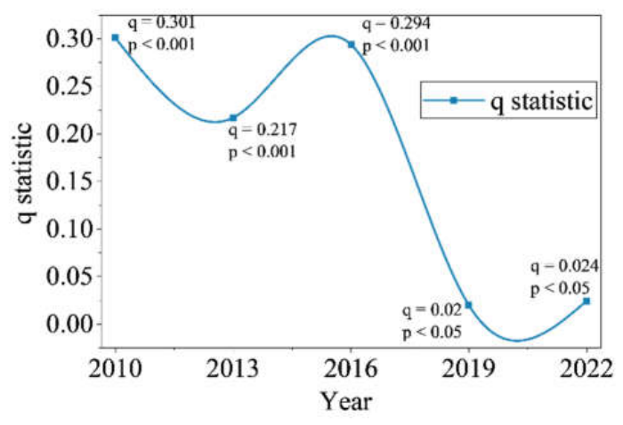
The Mann-Kendall trend test(Table 10) further reveals that the period-specific q-values for DEI, the year-specific q-values for CCD, the median TSFCI, the median CCD, and the median DEI all fail to reach statistical significance at the 0.05 level, indicating that none of these variables exhibit a significant monotonic trend—either upward or downward—over the study period. For the period-specific q-values of DEI, Kendall’s τ is -0.67, the Theil-Sen slope is -0.07, and the p-value is 0.33, suggesting a directional inclination toward declining explanatory power of TSFCI for DEI; however, given the lack of statistical significance, this cannot be interpreted as a stable unidirectional downward trend. For the year-specific q-values of CCD, Kendall’s τ is -0.60, the Theil-Sen slope is -0.077, and the p-value is 0.23, likewise failing the significance test. This implies that, despite a pronounced decline after 2019, the complete temporal sequence should still be characterized as exhibiting phased fluctuations rather than a significant unidirectional downward trend. In summary, the Mann-Kendall test outcomes corroborate the findings derived from the geographical detector analysis: the temporal association between TSFCs and the synergy between economic growth and carbon emission is characterized by temporal heterogeneity, yet no stable unidirectional trend of intensification or attenuation is present.
Table 10.
The Time-segmented Geodetector Results of DEI by TSFC.
| Phase | Effective sample size | The amount of TSFC classifications | q statistic | F statistic | p value | significance |
| 2010—2013 | 183 | 5 | 0.254 | 15.861 | 2e-4 | *** |
| 2013—2016 | 183 | 5 | 0.065 | 3.434 | 9.9e-2 | ** |
| 2016—2019 | 183 | 5 | 0.118 | 6.472 | 1e-4 | *** |
| 2019—2022 | 183 | 7 | 0.030 | 2.217 | 4.4e-2 | * |
Note:*** denotes extremely significant, ** denotes very significant, * denotes significant.
Table 10.
results of Mann-Kendall trend test.
| Inspection object | Kendall’s τ | p value | Theil-Sen coefficient | Trends |
| Period-specific q-values for DEI | -0.67 | 0.33 | -0.07 | No significant linear trend |
| Year-specific q-values for CCD | -0.60 | 0.23 | -0.077 | No significant linear trend |
| Median TSFCI (annual mean) | -0.53 | 0.21 | -0.53 | No significant linear trend |
| Median CCD (annual mean) | -0.80 | 0.08 | -0.80 | No significant linear trend |
| Median DEI (period mean) | 0.00 | 1.00 | 0.00 | No significant linear trend |
In summary, from the temporal dimension, the association between TSFCs and the synergy between economic growth and carbon emission is characterized by the coexistence of stage-specific stability and fluctuation. On the one hand, the explanatory power of TSFCI for DEI passes the significance test across all four consecutive periods, and its explanatory power for CCD reaches significant levels in all five years, indicating that TSFCs are indeed an important spatial factor influencing the county-level economic-environmental synergy in Sichuan Province. On the other hand, for both DEI and CCD, the q-values exhibit no trend of continuous increase or decrease over time; instead, they show pronounced fluctuations across different periods or years. Notably, after 2019, the explanatory power of TSFCI for both CCD and DEI declined to relatively low levels, suggesting that the influence of TSFCs on the synergy between economic growth and carbon emission weakened in the later period. However, this weakening does not imply the disappearance of the relationship, as the explanatory power of TSFCI for CCD in 2019 and 2022 still passed the significance test. This indicates that, in the later stage, the decoupling state and coupling coordination level may have been jointly influenced by multiple factors, including macroeconomic fluctuations, industrial structure adjustment, energy consumption changes, and external shocks. Therefore, the association between TSFCs and the contradiction between economic growth and carbon emission cannot be understood as a simple linear process; rather, it should be characterized as a dynamic process with significant spatial association, phased fluctuations, and nonlinear evolutionary characteristics.
4. Discussion
4.1. The Relationship Between TSFCs and the Contradiction of Economic Growth and Carbon Emission
Based on county-level data of Sichuan Province from 2010 to 2022, this study investigates the spatiotemporal association between territorial spatial functional conflicts (TSFCs) and the synergy between economic growth and carbon emission reduction from both spatial and temporal dimensions. The results show that the territorial spatial function conflict index (TSFCI) has significant explanatory power for the spatial heterogeneity of both the coupling coordination degree (CCD) and the decoupling elasticity index (DEI) (q = 0.081 and 0.023, respectively, p < 0.001), and there are obvious hierarchical differences in the economic-environmental synergy levels across regions with different conflict intensities.
However, TSFCI has limited explanatory power, with only a 2.30% explanatory rate for DEI over the entire study period. This indicates that TSFCs are an important correlative factor but not a decisive driving force. The relationship between economic growth and carbon emissions is jointly shaped by multiple factors including industrial structure, energy mix, technological progress, and ecological background. Theoretically, by altering land development intensity, ecological space stability, carbon source-sink patterns, and regional development pathways, TSFCs may exert a significant but limited spatial constraint on the economic-carbon synergy.
This finding provides empirical support for alleviating the “growth-emission reduction” contradiction through territorial spatial governance. Unlike existing studies that focus on single perspectives of land use or carbon emissions, this study integrates TSFCs into the analytical framework of economic-carbon synergy, proving that optimizing the allocation of territorial spatial functions and mitigating conflicts among production-living-ecological spaces is an important governance pathway to promote regional low-carbon transition and coordinated development.
Notably, the production-based territorial accounting adopted in this study means the observed economic-carbon contradiction reflects local production-side pressure. Against the background of industrial transfer from eastern China, inter-regional carbon leakage in Sichuan partly accounts for the limited explanatory power of TSFCs, as the contradiction is driven by both local spatial allocation and external consumption demand. Therefore, optimizing territorial spatial patterns can alleviate the production-side contradiction, while fundamental resolution requires cross-regional collaborative governance.
4.2. Spatial Mechanisms Underlying the Association Between TSFCs and the Economic-Environmental Synergy
Territorial spatial functional conflicts (TSFCs) in Sichuan Province exhibit a pronounced spatial differentiation pattern of “high in the basin, low in western Sichuan”. High-conflict areas are concentrated in the Chengdu Plain Economic Zone, Southern Sichuan Economic Zone, and urban agglomerations in northeastern Sichuan, while low-conflict areas are mainly distributed in the western Sichuan ecological barrier regions including Ganzi, Aba, and Ya’an. This pattern is highly consistent with Sichuan’s “west ecology – east economy” territorial spatial structure, indicating that population density, industrial agglomeration, and construction development intensity are highly coupled with the spatial pattern of TSFCs.
This spatial matching pattern provides a factual basis for interpreting the association between TSFCs and economic-carbon synergy. In basin and urbanized areas, construction land expansion and the concentration of industries and population intensify competition among production-living-ecological spaces. Theoretically, while high-intensity development drives short-term economic growth, it increases carbon emission pressure and compresses carbon sink capacity, thereby weakening synergy levels. In contrast, although western Sichuan ecological zones have low conflict levels, their weak economic foundations lead to a “low conflict – low synergy” paradox. Thus, low conflict does not equal high synergy, nor does high conflict necessarily correspond to the worst synergy state.
The study further reveals a nonlinear hierarchical relationship between TSFCs and synergy: neither the coupling coordination degree (CCD) nor the decoupling elasticity index (DEI) changes monotonically with conflict intensity. Moderate-conflict regions, with balanced development intensity and ecological constraints, are more likely to achieve a dynamic balance between development and protection (e.g., regions with TSFCI level 6 have the highest average DEI). Low-conflict regions often suffer from insufficient synergy due to underdevelopment, while high-conflict regions tend to accumulate structural contradictions from over-development.
Therefore, territorial spatial governance should not pursue “uniform conflict reduction across all regions” but shift to “optimizing conflict structure and improving the development-protection match”. High-conflict regions should strictly control construction land expansion and promote industrial low-carbon transformation; moderate-conflict regions should maintain the balance between development and protection; low-conflict yet low-synergy regions should enhance synergy through the value realization of ecological products and green industry cultivation.
4.3. Differences Between Static Coupling Coordination and Dynamic Decoupling Responses
This study employs both the coupling coordination degree (CCD) and decoupling elasticity index (DEI) to characterize the synergy between economic growth and carbon emissions. CCD is a static indicator reflecting the overall coordination level of the economic and carbon emission systems at a specific time point, while DEI is a dynamic indicator measuring the elastic relationship between changes in the economy and carbon emissions over adjacent periods. In this study, CCD was calculated for five time points (2010, 2013, 2016, 2019, 2022), and DEI was estimated for four consecutive periods (2010–2013, 2013–2016, 2016–2019, 2019–2022).
Full-period analysis shows that the territorial spatial function conflict index (TSFCI) has stronger explanatory power for the spatial heterogeneity of CCD. CCD is shaped by long-term territorial spatial patterns and stable factors such as economic scale, total carbon emissions, and regional development foundations, exhibiting strong spatial stability. In contrast, DEI is susceptible to short-term economic fluctuations, industrial cycles, energy consumption changes, policy adjustments, and external shocks. When data from multiple periods are pooled, these fluctuations dilute the overall strength of association between TSFCI and DEI.
Period-specific results further reveal pronounced phased characteristics in the statistical association between TSFCs and dynamic decoupling. The q-values for each period are 0.254 (2010–2013), 0.065 (2013–2016), 0.118 (2016–2019), and 0.030 (2019–2022), all statistically significant at the p < 0.05 level. This indicates that the influence intensity of TSFCs varies with development stages, policy environments, and macroeconomic conditions.
During periods of rapid economic expansion or drastic adjustment of territorial development patterns, spatial conflict patterns are more closely aligned with decoupling outcomes, alongside processes of construction land expansion, industrial restructuring, and ecological space compression. In contrast, during economic slowdowns, strengthened regulation, or external shocks, macroeconomic and industrial adjustments become the dominant factors, reducing the explanatory power of TSFCs. Therefore, the low full-period explanatory power of TSFCI for DEI does not negate the role of TSFCs, but rather indicates their significant phase sensitivity.
4.4. Temporal Evolution Characteristics: Phased Fluctuations Rather Than a Unidirectional Trend
The Mann-Kendall trend test shows that neither the period-specific q-values for DEI and year-specific q-values for CCD, nor the time series of TSFCI, CCD, and DEI themselves exhibit significant linear trends. This confirms that the strength of the association between TSFCs and economic-carbon synergy is not a unidirectional process of continuous strengthening or weakening, but rather manifests as phased fluctuations.
Analyses based on a single year or period would lead to one-sided conclusions. The marked decline in TSFCI’s explanatory power after 2019 does not mean its role has disappeared, but rather reflects that the economic-carbon synergy was influenced by more overlapping external factors during this stage. Meanwhile, the decrease in the proportion of strong decoupling and increase in recessive decoupling from 2019 to 2022 also indicate insufficient stability of low-carbon transition and increased volatility of regional development patterns in some areas of Sichuan Province.
In summary, the temporal dimension finding is summarized as “phased fluctuations with no significant overall linear trend”. This implies that territorial spatial conflict governance cannot rely on one-time static control, but requires the establishment of dynamic monitoring and phased regulation mechanisms to flexibly adjust development intensity, ecological control requirements, and low-carbon transition paths according to different development stages.
4.5. Policy Implications
Based on the above findings, the following territorial spatial governance recommendations are proposed for Sichuan Province and similar regions with complex terrain:
(1) Incorporate TSFCs into the overall governance framework. The territorial spatial development and conservation pattern is closely related to regional low-carbon development performance. Therefore, “dual carbon” governance should not only focus on energy structure optimization and industrial emission reduction, but also take into account territorial spatial function allocation, construction land expansion, ecological space protection, and carbon sink maintenance.
(2) Implement differentiated governance based on conflict levels. High-conflict regions should strictly control uncontrolled construction land expansion, revitalize stock land, promote green transformation of energy-intensive industries, and firmly uphold ecological bottom lines. Moderate-conflict regions should maintain the balance between development and protection to prevent further escalation of conflicts. Low-conflict regions should not blindly restrict development, but should simultaneously enhance economic strength and ecological benefits through the value realization of ecological products, green industry cultivation, and infrastructure improvement.
(3) Establish a phased dynamic monitoring system. Given the fluctuating strength of association between spatial conflicts and economic-carbon synergy, static planning cannot adapt to development needs. It is recommended to integrate TSFCI, CCD, and DEI into the monitoring and evaluation system of territorial spatial planning and “dual carbon” goals to track changes in spatial conflicts and their covariation with economic-environmental synergy in real time.
4.6. Limitations and Future Research Directions
First, the geographical detector can only identify the explanatory power of factors for spatial heterogeneity and cannot strictly establish causal relationships. The mechanistic inferences in this paper are mainly based on spatial statistical associations and existing theoretical frameworks. Throughout the paper, descriptions of the relationship between TSFCs and economic-carbon synergy strictly distinguish statistical correlation from causal inference, and all conclusions about exacerbation effects remain theoretical hypotheses. In addition, the geographical detector is sensitive to the discretization scheme of continuous independent variables. Although we adopted a consistent equal-interval classification method and verified the robustness of core conclusions through multiple discretization schemes, the absolute value of q-statistics may still be affected by the number of categories and boundary settings. Future research can further validate the results by combining spatial econometric models, panel causal inference methods, or scenario simulation approaches.
Second, this study uses county-level administrative units as the basic analytical units, which facilitates policy implementation but is susceptible to scale effects and the modifiable areal unit problem (MAUP). Future research can conduct multi-scale comparative analyses at the prefectural, grid, and watershed levels to test the robustness of the conclusions.
Third, this study mainly analyzes the relationship from the perspective of economic output and carbon emissions, without fully incorporating mediating variables such as industrial structure, energy mix, technological level, and ecological restoration investment. Subsequent research can use interaction detectors, multi-factor geographical detectors, or structural equation models to clarify the specific pathways through which TSFCs affect the contradiction between economic growth and carbon emission reduction.
Fourth, the TSFCI constructed in this study measures functional conflict intensity from the landscape pattern perspective, which mainly captures the structural conflict of spatial function allocation. It cannot fully cover the institutional and stakeholder dimensions of TSFCs derived from political ecology and land system science, such as interest games among multiple subjects and institutional arrangement deviations. Future research can integrate socio-economic statistics and stakeholder surveys to build a more comprehensive measurement system combining pattern structure and behavioral process.
Fifth, this study adopts production-based carbon emission accounting based on territorial boundaries, and does not include consumption-side carbon emissions and inter-provincial carbon transfer. For Sichuan Province, which undertakes industrial transfer, the production-side contradiction cannot fully reflect the real carbon emission responsibility of the region. Future research can combine multi-regional input-output models to expand the analysis from the consumption perspective, so as to more comprehensively identify the formation mechanism of the growth-emission reduction contradiction.
5. Conclusions
This study takes Sichuan Province, China, as the study area. Based on county-scale data from 2010 to 2022, it comprehensively employs landscape pattern indices, the coupling coordination degree model, the Tapio decoupling model, the geographical detector, the time-stratified geographical detector, and the Mann-Kendall trend test to investigate the spatiotemporal association between TSFC intensity and the synergy between economic growth and carbon emission from both spatial and temporal dimensions. The main conclusions are as follows.
(1) From 2010 to 2022, TSFCs in Sichuan Province exhibited pronounced spatial differentiation, generally characterized by a pattern of “high in the basin, low in western Sichuan.” High conflict levels were persistently observed in the Chengdu Plain Economic Zone, the Southern Sichuan Economic Zone, and some cities in northeastern Sichuan, while relatively low conflict levels were found in the western Sichuan ecological barrier regions, including Ganzi, Aba, and Ya’an. This pattern is largely consistent with Sichuan’s “west ecology – east economy” territorial spatial structure, indicating that population agglomeration, industrial activities, and development intensity are closely coupled with the spatial differentiation of TSFCs.
(2) The synergy between economic growth and carbon emission in Sichuan Province exhibited pronounced spatial heterogeneity and phased fluctuations. The CCD results indicate that most regions in Sichuan Province remain at a relatively low coordination stage between economic growth and net carbon emissions. The DEI results show that a certain decoupling trend emerged during the study period, but with significant differences across periods. The proportion of strong decoupling was relatively high from 2010 to 2019, while from 2019 to 2022, the proportion of strong decoupling decreased and the proportion of recession decoupling increased, indicating that the synergy between economic growth and carbon emission fluctuated in some regions during the later period, and the stability of the low-carbon transition remains insufficient.
(3) TSFCs have significant but limited spatial explanatory power for the synergy between economic growth and carbon emission. The full-region single-factor geographical detector results show that the q-values of TSFCI for CCD and DEI are 0.081 and 0.023, respectively, both passing the significance test. This indicates that TSFCI levels can significantly explain the spatial heterogeneity of county-level economic-environmental synergy, but their explanatory power is not strong. Therefore, TSFCI should be regarded as one of the important factors influencing the synergy between economic growth and carbon emission, rather than the sole or decisive factor.
(4) The impact of TSFCs is distinctly nonlinear and phased. Across different TSFCI levels, CCD and DEI do not exhibit simple linear changes but rather show hierarchical differentiation. The time-stratified geographical detector results reveal that the explanatory power of TSFCI for DEI was strongest from 2010 to 2013, declined from 2013 to 2016, rebounded from 2016 to 2019, and declined again from 2019 to 2022 while remaining significant. The explanatory power of TSFCI for CCD also exhibited a phased pattern of being stronger in the early period and markedly weaker in the later period. The Mann-Kendall trend test shows that the period-specific q-values for DEI, the year-specific q-values for CCD, and the temporal series of TSFCI, CCD, and DEI all exhibit no significant linear trends, indicating that the impact process is not one of continuous strengthening or weakening but rather manifests as phased fluctuations.
(5) This study confirms a significant spatiotemporal correlation between TSFC intensity and the degree of imbalance between economic growth and carbon emission reduction. Regions with higher TSFC intensity generally correspond to poorer economic-carbon synergy, and this correlation exhibits phased fluctuations and nonlinear characteristics. Optimizing territorial spatial development and conservation patterns to coordinate functional conflicts provides a feasible analytical perspective for alleviating the growth-emission reduction contradiction, and offers theoretical implications for promoting regional low-carbon transition and high-quality development.
Supplementary Materials
The following supporting information can be downloaded at the website of this paper posted on Preprints.org.
Author Contributions
Conceptualization, K.R. and D.O.; methodology, K.R. and D.O.; software, K.R.; validation, K.R.; formal analysis, K.R.; investigation, K.R. and Y.L.; resources, D.O. and J.X.; data curation, K.R.; writing—original draft preparation, K.R.; writing—review and editing, K.R. and Y.L.; visualization, K.R.; supervision, D.O. and J.X.; project administration, D.O. and J.X.; funding acquisition, D.O. and J.X. All authors have read and agreed to the published version of the manuscript.
Funding
This research was Supported by Open Fund of Observation and Research Station of Land Ecology and Land Use in Chengdu Plain, Ministry of Natural Resources, grant number CDORS-2024-06”.
Data Availability Statement
The raw data supporting the conclusions of this article will be made available by the authors on request.
Conflicts of Interest
The authors declare no conflicts of interest.
Appendix A
Table A1.
The average and median of TSFC Index of various urban areas in Sichuan Province.
| TSFC Index(Average) | TSFC Index(median) | |||||||||
|---|---|---|---|---|---|---|---|---|---|---|
| City | 2010 | 2013 | 2016 | 2019 | 2022 | 2010 | 2013 | 2016 | 2019 | 2022 |
| Leshan | 0.685 | 0.715 | 0.686 | 0.516 | 0.524 | 0.702 | 0.726 | 0.704 | 0.529 | 0.538 |
| Neijiang | 0.727 | 0.739 | 0.726 | 0.804 | 0.802 | 0.732 | 0.743 | 0.732 | 0.828 | 0.824 |
| Liangshan | 0.619 | 0.633 | 0.593 | 0.421 | 0.435 | 0.596 | 0.633 | 0.59 | 0.372 | 0.391 |
| Nanchong | 0.745 | 0.762 | 0.745 | 0.774 | 0.771 | 0.757 | 0.772 | 0.757 | 0.779 | 0.775 |
| Yibin | 0.743 | 0.761 | 0.744 | 0.682 | 0.682 | 0.76 | 0.775 | 0.76 | 0.717 | 0.715 |
| Bazhong | 0.756 | 0.777 | 0.757 | 0.66 | 0.659 | 0.771 | 0.788 | 0.772 | 0.708 | 0.706 |
| Guangyuan | 0.744 | 0.767 | 0.745 | 0.615 | 0.618 | 0.76 | 0.779 | 0.76 | 0.651 | 0.654 |
| Guangan | 0.685 | 0.702 | 0.686 | 0.743 | 0.741 | 0.701 | 0.716 | 0.701 | 0.802 | 0.795 |
| Deyang | 0.681 | 0.7 | 0.679 | 0.704 | 0.7 | 0.687 | 0.702 | 0.686 | 0.785 | 0.78 |
| Chengdu | 0.682 | 0.701 | 0.681 | 0.678 | 0.671 | 0.695 | 0.709 | 0.693 | 0.747 | 0.736 |
| PanzhiHua | 0.642 | 0.677 | 0.644 | 0.498 | 0.508 | 0.652 | 0.687 | 0.654 | 0.501 | 0.514 |
| Luzhou | 0.731 | 0.682 | 0.658 | 0.603 | 0.606 | 0.757 | 0.763 | 0.746 | 0.685 | 0.688 |
| Ganzi | 0.555 | 0.609 | 0.557 | 0.295 | 0.307 | 0.551 | 0.606 | 0.553 | 0.279 | 0.29 |
| Meishan | 0.704 | 0.726 | 0.704 | 0.68 | 0.683 | 0.727 | 0.741 | 0.727 | 0.759 | 0.759 |
| Mianyang | 0.694 | 0.723 | 0.694 | 0.583 | 0.585 | 0.721 | 0.742 | 0.722 | 0.648 | 0.648 |
| Zigong | 0.749 | 0.76 | 0.747 | 0.804 | 0.802 | 0.753 | 0.764 | 0.751 | 0.816 | 0.812 |
| Ziyang | 0.709 | 0.72 | 0.708 | 0.823 | 0.815 | 0.717 | 0.727 | 0.717 | 0.834 | 0.824 |
| Dazhou | 0.722 | 0.742 | 0.723 | 0.651 | 0.655 | 0.736 | 0.753 | 0.736 | 0.679 | 0.681 |
| Suining | 0.736 | 0.751 | 0.736 | 0.77 | 0.764 | 0.754 | 0.767 | 0.753 | 0.782 | 0.776 |
| Aba | 0.561 | 0.611 | 0.561 | 0.303 | 0.314 | 0.551 | 0.606 | 0.553 | 0.279 | 0.29 |
| Yaan | 0.604 | 0.649 | 0.606 | 0.388 | 0.398 | 0.553 | 0.607 | 0.555 | 0.296 | 0.307 |
Appendix B
Table A2.
CCD of GDP and net carbon emissions in cities (prefectures).
| City | mean | median | ||||||||
|---|---|---|---|---|---|---|---|---|---|---|
| 2010 | 2013 | 2016 | 2019 | 2022 | 2010 | 2013 | 2016 | 2019 | 2022 | |
| LeShan | 0.263 | 0.264 | 0.260 | 0.253 | 0.259 | 0.230 | 0.229 | 0.226 | 0.220 | 0.226 |
| NeiJiang | 0.283 | 0.285 | 0.280 | 0.273 | 0.278 | 0.238 | 0.239 | 0.236 | 0.230 | 0.235 |
| LiangShan | 0.240 | 0.239 | 0.235 | 0.229 | 0.235 | 0.230 | 0.229 | 0.226 | 0.221 | 0.226 |
| NanChong | 0.267 | 0.268 | 0.263 | 0.257 | 0.262 | 0.231 | 0.229 | 0.226 | 0.221 | 0.226 |
| YiBin | 0.252 | 0.252 | 0.248 | 0.242 | 0.248 | 0.230 | 0.229 | 0.226 | 0.220 | 0.225 |
| BaZhong | 0.243 | 0.243 | 0.239 | 0.233 | 0.239 | 0.231 | 0.229 | 0.226 | 0.220 | 0.226 |
| GuangYuan | 0.254 | 0.254 | 0.249 | 0.243 | 0.249 | 0.230 | 0.229 | 0.226 | 0.220 | 0.226 |
| GuangAn | 0.278 | 0.278 | 0.273 | 0.267 | 0.271 | 0.230 | 0.229 | 0.226 | 0.220 | 0.226 |
| DeYang | 0.347 | 0.349 | 0.344 | 0.336 | 0.340 | 0.273 | 0.272 | 0.270 | 0.263 | 0.266 |
| ChengDu | 0.403 | 0.406 | 0.399 | 0.392 | 0.395 | 0.304 | 0.307 | 0.302 | 0.294 | 0.297 |
| PanZhihua | 0.298 | 0.298 | 0.293 | 0.286 | 0.291 | 0.231 | 0.229 | 0.226 | 0.220 | 0.226 |
| LuZhou | 0.251 | 0.251 | 0.247 | 0.241 | 0.246 | 0.230 | 0.229 | 0.226 | 0.221 | 0.225 |
| GanZi | 0.232 | 0.231 | 0.227 | 0.221 | 0.227 | 0.231 | 0.229 | 0.225 | 0.219 | 0.226 |
| MeiShan | 0.273 | 0.274 | 0.270 | 0.264 | 0.268 | 0.230 | 0.229 | 0.226 | 0.221 | 0.226 |
| MianYang | 0.264 | 0.264 | 0.260 | 0.253 | 0.259 | 0.231 | 0.229 | 0.226 | 0.220 | 0.225 |
| ZiGong | 0.269 | 0.270 | 0.265 | 0.259 | 0.264 | 0.230 | 0.229 | 0.226 | 0.221 | 0.226 |
| ZiYang | 0.259 | 0.262 | 0.258 | 0.251 | 0.257 | 0.231 | 0.229 | 0.225 | 0.220 | 0.226 |
| DaZhou | 0.256 | 0.256 | 0.251 | 0.245 | 0.251 | 0.230 | 0.229 | 0.226 | 0.220 | 0.225 |
| SuiNing | 0.287 | 0.289 | 0.284 | 0.277 | 0.282 | 0.230 | 0.229 | 0.226 | 0.221 | 0.226 |
| ABa | 0.234 | 0.233 | 0.229 | 0.223 | 0.229 | 0.230 | 0.229 | 0.225 | 0.219 | 0.225 |
References
- Foley, J.A.; DeFries, R.; Asner, G.P.; Barford, C.; Bonan, G.; Carpenter, S.R.; Chapin, F.S.; Coe, M.T.; Daily, G.C.; Gibbs, H.K.; et al. Global Consequences of Land Use. Science 2005, 309, 570–574. [Google Scholar] [CrossRef] [PubMed]
- Intergovernmental Panel On Climate Change. Climate Change and Land: IPCC Special Report on Climate Change, Desertification, Land Degradation, Sustainable Land Management, Food Security, and Greenhouse Gas Fluxes in Terrestrial Ecosystems, 1st ed.; Cambridge University Press, 2022; ISBN 978-1-009-15798-8. [Google Scholar]
- Lambin, E.F.; Geist, H.J.; Lepers, E. Dynamics of Land-Use and Land-Cover Change in Tropical Regions. Annu. Rev. Environ. Resour. 2003, 28, 205–241. [Google Scholar] [CrossRef]
- Wu, J. Landscape Sustainability Science: Ecosystem Services and Human Well-Being in Changing Landscapes. Landsc. Ecol. 2013, 28, 999–1023. [Google Scholar] [CrossRef]
- Seto, K.C.; Güneralp, B.; Hutyra, L.R. Global Forecasts of Urban Expansion to 2030 and Direct Impacts on Biodiversity and Carbon Pools. Proc. Natl. Acad. Sci. 2012, 109, 16083–16088. [Google Scholar] [CrossRef] [PubMed]
- Liu, Y.; Fang, F.; Li, Y. Key Issues of Land Use in China and Implications for Policy Making. Land Use Policy 2014, 40, 6–12. [Google Scholar] [CrossRef]
- Grimm, N.B.; Faeth, S.H.; Golubiewski, N.E.; Redman, C.L.; Wu, J.; Bai, X.; Briggs, J.M. Global Change and the Ecology of Cities. Science 2008, 319, 756–760. [Google Scholar] [CrossRef] [PubMed]
- Friedlingstein, P.; O’Sullivan, M.; Jones, M.W.; Andrew, R.M.; Hauck, J.; Olsen, A.; Peters, G.P.; Peters, W.; Pongratz, J.; Sitch, S.; et al. Global Carbon Budget 2020. Earth Syst. Sci. Data 2020, 12, 3269–3340. [Google Scholar] [CrossRef]
- Zou, L.; Liu, Y.; Wang, J.; Yang, Y. An Analysis of Land Use Conflict Potentials Based on Ecological-Production-Living Function in the Southeast Coastal Area of China. Ecol. Indic. 2021, 122, 107297. [Google Scholar] [CrossRef]
- Xiao, P.; Xu, J.; Zhao, C. Conflict Identification and Zoning Optimization of “Production-Living-Ecological” Space. Int. J. Environ. Res. Public. Health 2022, 19, 7990. [Google Scholar] [CrossRef] [PubMed]
- Hou, Y.; Zhang, Z.; Wang, Y.; Sun, H.; Xu, C. Function Evaluation and Coordination Analysis of Production–Living–Ecological Space Based on the Perspective of Type–Intensity–Connection: A Case Study of Suzhou, China. Land 2022, 11, 1954. [Google Scholar] [CrossRef]
- Zheng, W.; Guo, B.; Su, H.; Liu, Z. Study on Multi-Scenarios Regulating Strategy of Land Use Conflict in Urban Agglomerations under the Perspective of “Three-Zone Space”: A Case Study of Harbin-Changchun Urban Agglomerations, China. Front. Environ. Sci. 2024, 11, 1288933. [Google Scholar] [CrossRef]
- Feng, Z.; Long, S.; Liu, Y. Spatial Conflicts in ‘Production, Living, and Ecological Space’ Functions at Urban Fringes: The Case of Zengcheng, Guangzhou. Appl. Sci. 2025, 15, 3483. [Google Scholar] [CrossRef]
- Xiong, J.; Yue, W.; Xia, H.; Wang, T.; Liu, Y.; Pijanowski, B.C. Will China’s Territorial Spatial Planning Policies Enhance Land Use Sustainability? An Integrated Assessment under Global Environmental Change. Resour. Environ. Sustain. 2025, 21, 100228. [Google Scholar] [CrossRef]
- Yu, Y.; Cao, X.; Ye, D.; Jiang, X. Critical Considerations in Provincial Territorial Spatial Planning in China: A Qualitative and Spatial Analysis. Humanit. Soc. Sci. Commun. 2025, 12, 1422. [Google Scholar] [CrossRef]
- Jiang, S.; Meng, J.; Zhu, L. Spatial and Temporal Analyses of Potential Land Use Conflict under the Constraints of Water Resources in the Middle Reaches of the Heihe River. Land Use Policy 2020, 97, 104773. [Google Scholar] [CrossRef]
- Long, H.; Qu, Y.; Tu, S.; Zhang, Y.; Jiang, Y. Development of Land Use Transitions Research in China. J. Geogr. Sci. 2020, 30, 1195–1214. [Google Scholar] [CrossRef]
- Huang, W.; Wang, Z.; Liu, Y.; Shi, J. Evolution Characteristics and Pattern Optimization of Land Use Conflict in Inland River Basin from the Perspective of Production-Living-Ecological. PLoS ONE 2025, 20, e0321481. [Google Scholar] [CrossRef] [PubMed]
- Turner, M.G. Landscape Ecology: The Effect of Pattern on Process. Annu. Rev. Ecol. Syst. 1989, 20, 171–197. [Google Scholar] [CrossRef]
- McGarigal, K.; Marks, B.J. FRAGSTATS: Spatial Pattern Analysis Program for Quantifying Landscape Structure; General Technical Report; USDA Forest Service: Portland, OR, USA, 1995. [Google Scholar]
- Uuemaa, E.; Mander, Ü.; Marja, R. Trends in the Use of Landscape Spatial Metrics as Landscape Indicators: A Review. Ecol. Indic. 2013, 28, 100–106. [Google Scholar] [CrossRef]
- Lambin, E.F.; Meyfroidt, P. Global Land Use Change, Economic Globalization, and the Looming Land Scarcity. Proc. Natl. Acad. Sci. 2011, 108, 3465–3472. [Google Scholar] [CrossRef] [PubMed]
- Chen, X.; Nordhaus, W.D. Using Luminosity Data as a Proxy for Economic Statistics. Proc. Natl. Acad. Sci. 2011, 108, 8589–8594. [Google Scholar] [CrossRef] [PubMed]
- Tapio, P. Towards a Theory of Decoupling: Degrees of Decoupling in the EU and the Case of Road Traffic in Finland between 1970 and 2001. Transp. Policy 2005, 12, 137–151. [Google Scholar] [CrossRef]
- Houghton, R.A.; Nassikas, A.A. Global and Regional Fluxes of Carbon from Land Use and Land Cover Change 1850–2015. Glob. Biogeochem. Cycles 2017, 31, 456–472. [Google Scholar] [CrossRef]
- Canadell, J.G.; Le Quéré, C.; Raupach, M.R.; Field, C.B.; Buitenhuis, E.T.; Ciais, P.; Conway, T.J.; Gillett, N.P.; Houghton, R.A.; Marland, G. Contributions to Accelerating Atmospheric CO2 Growth from Economic Activity, Carbon Intensity, and Efficiency of Natural Sinks. Proc. Natl. Acad. Sci. 2007, 104, 18866–18870. [Google Scholar] [CrossRef] [PubMed]
- Xiong, S.; Yang, F.; Zhang, J.; Tang, Y. An Integrated Model Chain for Diagnosing and Predicting Conflicts between Production-Living-Ecological Space in Lake Network Regions: A Case of the Dongting Lake Region, China. Ecol. Indic. 2024, 166, 112237. [Google Scholar] [CrossRef]
- Wang, J.-F.; Zhang, T.-L.; Fu, B.-J. A Measure of Spatial Stratified Heterogeneity. Ecol. Indic. 2016, 67, 250–256. [Google Scholar] [CrossRef]
- Song, Y.; Wang, J.; Ge, Y.; Xu, C. An Optimal Parameters-Based Geographical Detector Model Enhances Geographic Characteristics of Explanatory Variables for Spatial Heterogeneity Analysis: Cases with Different Types of Spatial Data. GIScience Remote Sens. 2020, 57, 593–610. [Google Scholar] [CrossRef]
- Wang, F.; Shao, W.; Yu, H.; Kan, G.; He, X.; Zhang, D.; Ren, M.; Wang, G. Re-Evaluation of the Power of the Mann-Kendall Test for Detecting Monotonic Trends in Hydrometeorological Time Series. Front. Earth Sci. 2020, 8, 14. [Google Scholar] [CrossRef]
- Then, Y.J.; Abdul Halim, S. Modified Mann-Kendall with Higher-Order Statistics for Trend Analysis. Sci. Rep. 2025, 16, 500. [Google Scholar] [CrossRef] [PubMed]
- Luo, H.; Zhang, Y.; Li, Y.; Liu, Z.; Gao, X.; Luo, X.; Shang, W.-L.; Yang, X.; Meng, X. Deciphering Land Use-Carbon Emissions-Economy Nexus: Decoupling Dynamics and Sustainable Planning Pathways. Nexus 2025, 2, 100088. [Google Scholar] [CrossRef]
- Chen, J.; Gao, M.; Cheng, S.; Hou, W.; Song, M.; Liu, X.; Liu, Y. Global 1 Km × 1 Km Gridded Revised Real Gross Domestic Product and Electricity Consumption during 1992–2019 Based on Calibrated Nighttime Light Data. Sci. Data 2022, 9, 202. [Google Scholar] [CrossRef] [PubMed]
- Jinchuan, H.U.A.N.G.; Haoxi, L.I.N.; Xiaoxiao, Q.; Jinchuan, H.; Haoxi, L.; Xiaoxiao, Q. A Literature Review on Optimization of Spatial Development Pattern Based on Ecological-Production-Living Space. Prog. Geogr. 2017, 36, 378–391. [Google Scholar] [CrossRef]
- SHAN, W.; Jing, X.B. Yin-kang Production-Living-Ecological” Function Evaluation and Coupling Coordination Analysis of Land Use in Jiangsu Province. Resour. Environ. YANGTZE BASIN 2019, 28, 1541. [Google Scholar] [CrossRef]
- Ren Jun Analysis on Spatial-Temporal Characteristics and Influencing Factors of Multi-Functionality of Land Use in Qinghai-Tibet Alpine Mountain Areas: A Case Study of Haidong City in Qinghai Province, China. China Land Sci. 2021, 35. [CrossRef]
- JIANG Xintong, Z.S.; Shiyan, Z.H.A.I.; Zheng, W.A.N.G.; Huan, L.I.U.; Jing, C.H.E.N.; Yueyue, Z.H.U. Simulating the Production-Living-Ecological Space and Analyzing Eco-Environmental Effects Based on FLUS Model in Zhengzhou, China. Acta Ecol. Sin. 2023, 43, 6225. [Google Scholar] [CrossRef]
- Basu, T.; Das, A. Urbanization Induced Changes in Land Use Dynamics and Its Nexus to Ecosystem Service Values: A Spatiotemporal Investigation to Promote Sustainable Urban Growth. Land Use Policy 2024, 144, 107239. [Google Scholar] [CrossRef]
- Liu, J.; Liu, Y.; Yan, M. Spatial and Temporal Change in Urban-Rural Land Use Transformation at Village Scale—A Case Study of Xuanhua District, North China. J. Rural Stud. 2016, 47, 425–434. [Google Scholar] [CrossRef]
- Lin, G.; Jiang, D.; Fu, J.; Cao, C.; Zhang, D. Spatial Conflict of Production–Living–Ecological Space and Sustainable-Development Scenario Simulation in Yangtze River Delta Agglomerations. Sustainability 2020, 12, 2175. [Google Scholar] [CrossRef]
- Zhou, D.; Lin, Z.; Lim, S.H. Spatial Characteristics and Risk Factor Identification for Land Use Spatial Conflicts in a Rapid Urbanization Region in China. Environ. Monit. Assess. 2019, 191, 677. [Google Scholar] [CrossRef] [PubMed]
- Jiang, S.; Meng, J.; Zhu, L.; Cheng, H. Spatial-Temporal Pattern of Land Use Conflict in China and Its Multilevel Driving Mechanisms. Sci. Total Environ. 2021, 801, 149697. [Google Scholar] [CrossRef] [PubMed]
- Ma, W.; Jiang, G.; Chen, Y.; Qu, Y.; Zhou, T.; Li, W. How Feasible Is Regional Integration for Reconciling Land Use Conflicts across the Urban–Rural Interface? Evidence from Beijing–Tianjin–Hebei Metropolitan Region in China. Land Use Policy 2020, 92, 104433. [Google Scholar] [CrossRef]
- Tang, L.; Wang, L.; Li, Q.; Zhao, J. A Framework Designation for the Assessment of Urban Ecological Risks. Int. J. Sustain. Dev. World Ecol. 2018, 25, 387–395. [Google Scholar] [CrossRef]
- Mcgarigal, K.S.; Cushman, S.A.; Neel, M.C.; Ene, E. FRAGSTATS: Spatial Pattern Analysis Program for Categorical Maps. 2002. Available online: www.umass.edu/landeco/research/fragstats/fragstats.html.
- Wu, T.; Zha, P.; Yu, M.; Jiang, G.; Zhang, J.; You, Q.; Xie, X. Landscape Pattern Evolution and Its Response to Human Disturbance in a Newly Metropolitan Area: A Case Study in Jin-Yi Metropolitan Area. Land 2021, 10, 767. [Google Scholar] [CrossRef]
- Wang, X.; Li, X.; Sha, J.; Zhang, H.; Shifaw, E.; Guo, X.; Lai, S.; Wang, J. Trade-Offs and Synergies for Urban Production-Living-Ecological Spatial Patterns-Comparison Study between Fuzhou, China, and Saskatoon, Canada. Ecol. Indic. 2024, 169, 112816. [Google Scholar] [CrossRef]
- Chen, S.; Chen, B.; Fath, B.D. Ecological Risk Assessment on the System Scale: A Review of State-of-the-Art Models and Future Perspectives. Ecol. Model. 2013, 250, 25–33. [Google Scholar] [CrossRef]
- OECD. European Union; Joint Research Centre - European Commission Handbook on Constructing Composite Indicators: Methodology and User Guide; OECD, 2008; ISBN 978-92-64-04345-9. [Google Scholar]
- Chuai, X.; Huang, X.; Wang, W.; Zhao, R.; Zhang, M.; Wu, C. Land Use, Total Carbon Emissions Change and Low Carbon Land Management in Coastal Jiangsu, China. J. Clean. Prod. 2015, 103, 77–86. [Google Scholar] [CrossRef]
- Zhao, X.; Zhang, X.; Shao, S. Decoupling CO 2 Emissions and Industrial Growth in China over 1993–2013: The Role of Investment. Energy Econ. 2016, 60, 275–292. [Google Scholar] [CrossRef]
Figure 2.
Conceptual framework of coupled TSFC and landscape ecological risk assessment.
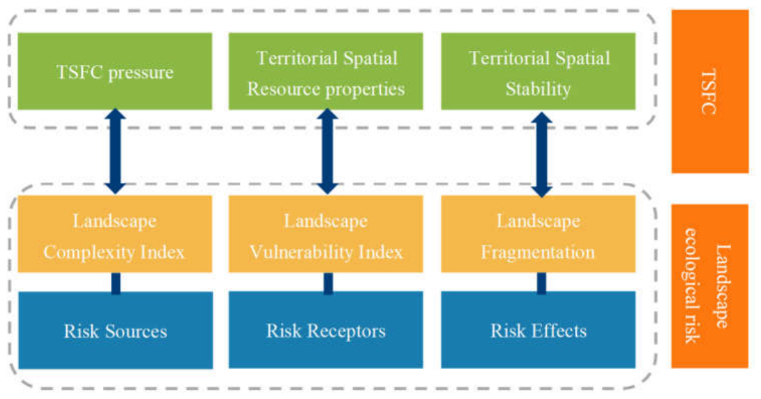
Figure 3.
Spatial distribution of TSFCI. (a) shows the TSFCI distribution in 2010, (b) shows the TSFCI distribution in 2013, (c) shows the TSFCI distribution in 2016, (d) shows the TSFCI distribution in 2019, and (e) shows the TSFCI distribution in 2022.
Figure 3.
Spatial distribution of TSFCI. (a) shows the TSFCI distribution in 2010, (b) shows the TSFCI distribution in 2013, (c) shows the TSFCI distribution in 2016, (d) shows the TSFCI distribution in 2019, and (e) shows the TSFCI distribution in 2022.
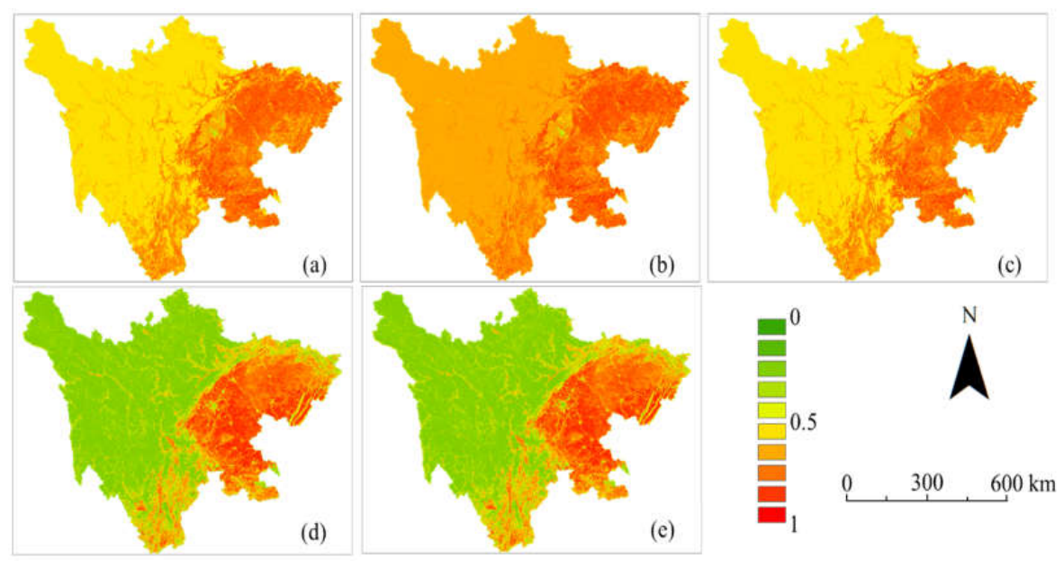
Figure 4.
Temporal changes of TSFCI in typical regions.
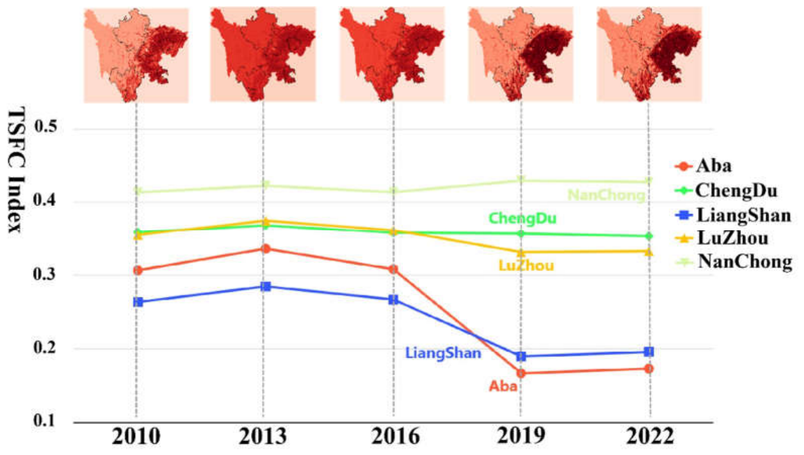
Figure 5.
Spatial Distribution of Annual Coupling Coordination Degree in Sichuan Province. (a) represents the coupling coordination degree in 2010, (b) represents the coupling coordination degree in 2013, (c) represents the coupling coordination degree in 2016, (d) represents the coupling coordination degree in 2019, and (e) represents the coupling coordination degree in 2022.
Figure 5.
Spatial Distribution of Annual Coupling Coordination Degree in Sichuan Province. (a) represents the coupling coordination degree in 2010, (b) represents the coupling coordination degree in 2013, (c) represents the coupling coordination degree in 2016, (d) represents the coupling coordination degree in 2019, and (e) represents the coupling coordination degree in 2022.
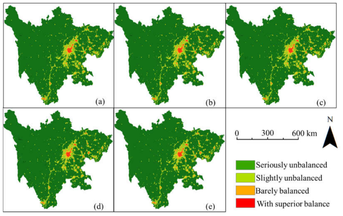
Figure 6.
Changes in the proportional structure of decoupling types across different stages. (It can be observed that from 2010 to 2019, strong decoupling (SD) accounted for a relatively high proportion. However, from 2019 to 2022, SD decreased significantly, and recession decoupling (RD) became the dominant type. This indicates that the decoupling state in Sichuan Province has gradually shifted from growth-oriented decoupling in the earlier period to recession-oriented decoupling in the later period.).
Figure 6.
Changes in the proportional structure of decoupling types across different stages. (It can be observed that from 2010 to 2019, strong decoupling (SD) accounted for a relatively high proportion. However, from 2019 to 2022, SD decreased significantly, and recession decoupling (RD) became the dominant type. This indicates that the decoupling state in Sichuan Province has gradually shifted from growth-oriented decoupling in the earlier period to recession-oriented decoupling in the later period.).
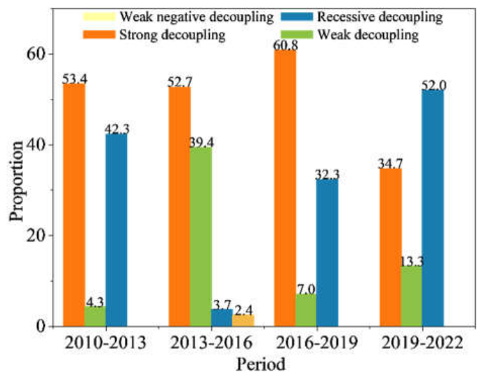
Figure 7.
Changes in SD and WD proportions in Chengdu, Nanchong, Luzhou, Liangshan, and Aba (2010–2022). (a) is Changes in Strong Decoupling Proportion. (b) is Weak Decoupling Proportion.
Figure 7.
Changes in SD and WD proportions in Chengdu, Nanchong, Luzhou, Liangshan, and Aba (2010–2022). (a) is Changes in Strong Decoupling Proportion. (b) is Weak Decoupling Proportion.
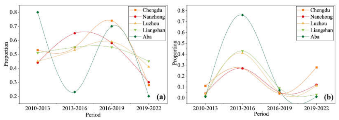
Table 1.
This is a table. Tables should be placed in the main text near to the first time they are cited.
Table 1.
This is a table. Tables should be placed in the main text near to the first time they are cited.
| Data type | Name | Time | Precision | Resource |
|---|---|---|---|---|
| Raster | Land change survey data of Sichuan Province | 2010-2022 | 120m | Sichuan Provincial Academy of Land Science and Technology (Sichuan Satellite Application Technology Center) |
| GDP | 2010-2022 | 1km | Chen et al.[33]. | |
| Vector | Administrative boundary of Sichuan Province | 2024 | National Platform for Common GeoSpatial Information Services(https://www.tianditu.gov.cn/) | |
| Statistical | Fossil energy consumption | 2010-2022 | “China Energy Statistical Yearbook” | |
| Forest fire area | 2010-2022 | “Sichuan Statistical Yearbook” | ||
| Crop yield | 2010-2022 | “Sichuan Statistical Yearbook” | ||
| Coal mining output | 2010-2022 | “China Energy Statistical Yearbook” | ||
| Oil and natural gas production | 2010-2022 | “China Energy Statistical Yearbook” | ||
| Industrial product output | 2010-2022 | “Sichuan Statistical Yearbook” | ||
| Livestock inventory | 2010-2022 | “Sichuan Statistical Yearbook” | ||
| Population size | 2010-2022 | “Sichuan Statistical Yearbook” | ||
| Rice planting area | 2010-2022 | “China Agricultural Statistical Yearbook” | ||
| Domestic waste landfill volume | 2010-2022 | “China Environmental Statistical Yearbook” | ||
| Domestic waste incineration volume | 2010-2022 | “China Environmental Statistical Yearbook” | ||
| COD emissions | 2010-2022 | “China Environmental Statistical Yearbook” |
Note: all grid data are resampled to a 1 km scale when participating in TSFC, CCD and DEI calculations.
Table 2.
Classification of Territorial Space.
| Primary class | Secondary class | Land use types |
| Urban Space (US) | Urban Production Space (UPS) | Mining land, port and wharf land, highway land, pipeline transport land, airport land, railway land |
| Urban Living Space (ULS) | Urban land, town land | |
| Rural Space (RS) | Rural Production Space (RPS) | Paddy fields, dry land, irrigated land, ridge land, canals, tea gardens, orchards, rural roads, other orchard land, agricultural facility land |
| Rural Living Space (RLS) | Village land | |
| Ecological Space (ES) | Natural Ecological Space (ES) | Hydraulic structure land, glaciers and permanent snow, scenic and special land, shrubland, river surfaces, lake surfaces, pond surfaces, bare land, inland mudflats, other grassland, other forestland, artificial pastureland, sandy land, reservoir surfaces, natural pastureland, saline-alkali land, forestland, marshland |
Table 3.
Classification of TSFCs.
| TSFC Index | Level | Note |
|---|---|---|
| 0.0-0.1 | 1 | Minimal |
| 0.1-0.2 | 2 | Very low |
| 0.2-0.3 | 3 | Low |
| 0.3-0.4 | 4 | Low to moderate |
| 0.4-0.5 | 5 | Moderate |
| 0.5-0.6 | 6 | Low to moderate |
| 0.6-0.7 | 7 | High |
| 0.7-0.8 | 8 | Very high |
| 0.8-0.9 | 9 | Severe |
| 0.9-1.0 | 10 | Extreme |
Table 4.
territorial carbon source and carbon sink inventory.
| Carbon budget | Department | Item |
| Carbon source | Department of Energy | Fossil fuel combustion |
| Forest fires | ||
| straw burning | ||
| coal mining fugitive emissions | ||
| oil and natural gas system fugitive emissions | ||
| Department of Industrial Processes and Product Usage | Industrial processes | |
| Department of Agriculture, Forestry and Other Land Use | Livestock enteric fermentation and manure management | |
| Breathing of humans and animals | ||
| rice cultivation | ||
| Department of Waste Processing | Solid waste treatment | |
| wastewater treatment | ||
| Carbon sink | Terrestrial ecosystem carbon sink | Forestland, grassland, water bodies |
Table 6.
Tapio decoupling types and their classification criteria.
| States | Indicators | ||
|---|---|---|---|
| ΔCO2 / CO2 | ΔGDP / GDP | DEI | |
| Strong decoupling | < 0 | > 0 | DEI < 0 |
| Weak decoupling | > 0 | > 0 | 0 < DEI < 0.8 |
| Recessive decoupling | < 0 | < 0 | DEI > 1.2 |
| Strong negative decoupling | > 0 | < 0 | DEI < 0 |
| Weak negative decoupling | < 0 | < 0 | 0 < DEI < 0.8 |
| Expansive negative decoupling | > 0 | < 0 | DEI > 1.2 |
| Expansive coupling | > 0 | > 0 | 0.8 < DEI < 1.2 |
| Recessive coupling | < 0 | < 0 | 0.8 < DEI < 1.2 |
Disclaimer/Publisher’s Note: The statements, opinions and data contained in all publications are solely those of the individual author(s) and contributor(s) and not of MDPI and/or the editor(s). MDPI and/or the editor(s) disclaim responsibility for any injury to people or property resulting from any ideas, methods, instructions or products referred to in the content. |
© 2026 by the authors. Licensee MDPI, Basel, Switzerland. This article is an open access article distributed under the terms and conditions of the Creative Commons Attribution (CC BY) license (http://creativecommons.org/licenses/by/4.0/).
Copyright: This open access article is published under a Creative Commons CC BY 4.0 license, which permit the free download, distribution, and reuse, provided that the author and preprint are cited in any reuse.


