

Submitted:
29 June 2026
Posted:
29 June 2026
You are already at the latest version
Abstract
In open-pit optimization software, metallurgical recovery is commonly treated as a constant for every block, although it varies with ore type and grade. Here, recovery is modelled as a block-grade-dependent variable using 24 laboratory flotation tests on the sulfide ore of a copper deposit in eastern Türkiye, and its effect on net present value (NPV) and the cut-off grade decision is examined. The deposit is split by sulfur content into two routes: sulfide ore (S ≥ 9%) to flotation and oxide ore (S < 9%) to heap leaching. Across a feed grade of 0.22–6.99% Cu, the measured recovery increases with feed grade from about 61% to 94%; the linear correlation is only moderate (r = 0.60), but the relationship is well described by a bounded, saturating recovery–grade curve (R(g) = R_max•g/(g + k); R_max = 0.95, k = 0.12; R² = 0.87). For the leach route, where no test data are available, a fixed 80% recovery is retained throughout. Optimization I (fixed recovery) and Optimization II (variable recovery on the sulfide route) are compared over ten scenarios, using a slope-constrained ultimate pit (50° overall slope, 5% discount rate). Because the deposit's copper is concentrated in high-grade sulfide blocks with measured recovery of about 90–93%, the metal-weighted recovery of the sulfide ore is 88.9%, and the fixed 80% assumption underestimates both recoverable copper and NPV. Under a fixed pit and cut-off, variable recovery yields roughly 8% higher NPV and about 2.9 kt more copper. When the cut-off grade is instead determined economically, variable recovery reclassifies the marginal low-grade sulfide ore (~0.05 Mt, measured recovery below 80%) as uneconomic; even so, total copper output rises from 40.2 kt (fixed) to 43.0 kt (variable) — a slightly smaller gain, because this marginal ore is excluded. Grade-dependent recovery derived from laboratory data thus determines both the recoverable metal and the marginal-ore boundary more realistically than a fixed assumption, and materially affects NPV for this deposit.
Keywords:
copper
; flotation
; direct block scheduling
; metallurgical recovery
; pit optimization
; net present value
; cut-off grade
1. Introduction
Mining ventures are capital-intensive activities whose long-term investment decisions must be made years before the associated cash flows are realised. Because of the natural variability of an ore deposit and the limited density of sampling, the geological data underlying these decisions carry inherent uncertainty [2,3], which propagates into economic evaluation, investment appraisal, and mine design [4]. Three-dimensional reserve optimization compounds this issue: the objective function and its parameters — selling price, costs, and metallurgical recovery — are each estimated rather than known, so the optimized pit and schedule inherit their uncertainty [1].
Among these parameters, metallurgical recovery is particularly often simplified. In most pit-optimization software it is entered as a single constant applied to every block over the entire mine life, even though recovery in practice varies with ore type and grade. Treating recovery as a block-independent constant therefore embeds a hidden bias in the recoverable-metal estimate, in the block economic value, and ultimately in net present value (NPV) and the cut-off grade decision. This study addresses that bias directly. Using grade-dependent recovery derived from 24 laboratory flotation tests on the sulfide ore of an open-pit copper deposit in eastern Türkiye, recovery is modelled as a block-level variable and incorporated into a slope-constrained pit optimization. By comparing this variable-recovery optimization against the conventional fixed-recovery case over a common set of scenarios, the study quantifies how much the constant-recovery assumption distorts NPV and the marginal-ore (cut-off) boundary for a real deposit.
2. Uncertainty in Metallurgical Recovery and Related Studies
Metallurgical recovery has been treated in the literature well beyond simple qualitative description. The value of analysing multivariate metal recovery and plant performance with rigorous statistical tools has been emphasised [7], and methods have been proposed to simulate grade and metallurgical recovery jointly at drill-hole locations so that recovery can be carried as a block attribute rather than a global average [8]. In a closely related experimental line, processing studies on chromite have shown that recovery is governed by feed characteristics rather than being a fixed property of the ore, so that a single constant recovery can misrepresent the recoverable metal [9].
Despite this evidence, many planning frameworks still rely on fixed recovery and fixed cost [10,11]. It has been demonstrated, however, that the recovery of an ore mass is not constant and that, under a fixed-cost assumption, recovery and capacity may themselves vary [12,13]. Building on this, a dynamic cut-off grade criterion has been advocated within the optimal production pattern [14], and metallurgical recovery and grinding performance have been shown to influence both planned production and the timing of cash flows [16]. More broadly, incorporating geometallurgical attributes and geological uncertainty into long-term planning — whether through multivariate resource models, stochastic optimization of mining complexes, or heuristic scheduling — yields more realistic economic outcomes than deterministic, single-value approaches [5,6,15,16,23].
Taken together, these studies establish that recovery is variable and that this variability matters economically. What remains largely unquantified, however, is the effect of a laboratory-derived, block-grade-dependent recovery on the NPV and the cut-off grade of a real open-pit copper deposit, relative to the constant-recovery assumption embedded in standard optimization software. The present work fills this gap: dynamic (variable) recovery obtained from flotation tests is applied block by block, the pit is re-optimized on this basis, and the outcome is compared directly with the conventional fixed-recovery case.
3. Constant Recovery Assumption and the Approach of the Study
The problem addressed here is how the choice of metallurgical-recovery model changes the optimized pit and its economics for the study deposit, with every other input held fixed. Each block i is characterised by its copper grade g_i (% Cu) and its sulfur content Si (% S), and these two attributes drive two separate decisions. First, the processing route is set by sulfur content: high-sulfur blocks are sulfidic and are sent to flotation, whereas low-sulfur blocks are oxidic and are sent to heap leaching. Using a site-specific operational threshold of 9% S,
Route(i) = sulfide (flotation), Si ≥ 9% ; Route(i) = oxide (leach), Si < 9%
Second — and only on the flotation route — the metallurgical recovery of a block is allowed to depend on its copper grade. The oxide route, for which no flotation test data exist, is assigned a constant recovery in all cases. On this basis, two recovery models are compared. In Optimization I (fixed recovery), every flotation block is assigned the same constant recovery — here 80%, as in conventional practice. In Optimization II (variable recovery), each flotation block is instead assigned the grade-dependent recovery R(g_i) obtained from the laboratory flotation tests (Section 4.1). Crucially, the recovery model applied to the sulfide route is the only quantity that changes between the two cases: in both optimizations the leach route keeps its fixed recovery, and the block model, prices, costs, slope constraints, discount rate, and production capacities are held identical. For each model the ultimate pit limit is solved, the blocks are scheduled, and the recoverable copper, the net present value (NPV), and the economic cut-off (marginal-ore) boundary are computed. Comparing these outputs isolates the effect of the constant-recovery assumption from every other modelling choice and quantifies its consequences for the economic evaluation of the deposit.
4. Methodology
4.1. Recovery Model Based on Grade from Flotation Tests
To characterise the concentration behaviour of the sulfide ore, 24 laboratory flotation tests were carried out. In a beneficiation circuit the copper mass balance over feed (F), concentrate (C), and tailing (T) is preserved [18,19]
where f, c, and t are the feed, concentrate, and tailing grades (% Cu), respectively. The metallurgical recovery R is the proportion of feed copper reporting to the concentrate [18]
F · f = C · c + T · t
R = (C · c) / (F · f) · 100
Because recovery is computed directly from the feed and concentrate assays (Eq. 3), it already reflects any copper lost to other streams. In practice three products form — concentrate, middling, and tailing — so the copper carried by the middling is not recovered; the measured recovery (mean 85.6%) therefore lies below the value that the idealised two-product balance (Eq. 2) would predict. The measured recovery, which already incorporates this middling loss, was used directly throughout.
Across the 24 tests the feed grade ranged over 0.22–6.99% Cu, the concentrate grade averaged 30.3% Cu, and the feed-to-tailing grade ratio (f/t) averaged 8.8. The measured recovery correlates positively with feed grade (r = 0.60; Table 6) and even more strongly with concentrate grade (r = 0.80). Recovery is nevertheless modelled as a function of feed grade, because in the block model only the in-situ (feed) grade of a block is known in advance; the concentrate grade is an outcome of processing, not a block attribute available for prediction. To capture the dependence of recovery on grade while respecting its physical bounds, an empirical saturating model was adopted rather than a linear regression. Recovery must be non-negative, must increase with grade, and cannot exceed 100%; a straight-line fit honours none of these limits at the extremes. A bounded, saturating function of the rectangular-hyperbola (Michaelis–Menten / Langmuir) type satisfies all three requirements and was therefore fitted to the data:
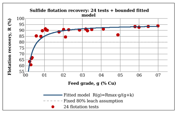
where R_max is the asymptotic (maximum attainable) recovery and k is the half-saturation grade at which R = R_max/2. The two parameters were estimated from the 24 test points by least squares, with R_max constrained not to exceed 100%; this gave R_max = 0.95, k = 0.12, and R² = 0.87 (Figure 1). The relationship is used purely as an empirical, physically constrained descriptor of the measured recovery–grade trend, not as a theoretically derived recovery law. The tests span 0.22–6.99% Cu and therefore cover essentially the full grade range of the sulfide blocks: only a negligible fraction of the sulfide copper (about 0.36%) lies above 6.99% Cu and is obtained by extrapolating the curve. For the oxide (leach) route, for which no flotation test data are available, a fixed recovery of 80% was retained in both optimizations.
R(g) = R_max · g / (g + k)
4.2. Slope Restricted Ultimate pit and Period Planning
In Micromine—as in comparable pit-optimization packages—metallurgical recovery does not act on the optimizer directly; it enters only through the recoverable metal, and hence the economic value, assigned to each block (Equation 6), which conventional practice supplies as a single global constant. Optimization II was therefore implemented by evaluating each block's recovery R(g_i) from the fitted grade–recovery curve and assigning it as a per-block attribute, so that the ultimate-pit (Lerchs–Grossmann) and NPV-based scheduling algorithms operate on block economic values that already embed the grade-dependent recovery; Optimization I uses the identical workflow with the recovery field held at the fixed 80%. The optimizer is agnostic to the origin of each block's value, which is what makes variable recovery implementable within software that conventionally assumes a single constant.
The economic optimization was carried out in Micromine in two linked stages: the ultimate pit defined the outer mining limit, and the blocks inside it were then scheduled directly into production periods. The ultimate pit limit was obtained by solving a maximum-closure problem under slope precedence constraints. An economic value v_i (Section 4.3) is assigned to each block i; for any valid closure Π — a set of blocks that satisfies the precedence constraints — the objective is
max Σ_{i∈Π} v_i , Π a closure satisfying the slope constraint
This problem was solved by Lerchs–Grossmann optimisation as implemented in Micromine [21]. The slope constraint was imposed through a precedence pattern corresponding to a 50° overall slope angle obtained from a geotechnical slope optimisation for the deposit; a block may be extracted only after the overlying blocks defined by this pattern.
Within the ultimate pit, production was scheduled with Micromine's net-present-value scheduler, which assigns individual blocks directly to annual periods — rather than through predefined pushbacks — so as to maximise discounted value. The schedule honours the same slope precedence and is bounded by the annual mining and processing capacities (Section 4.4); the resulting period cash flows CF_t give the NPV (Eq. 10). This direct block-scheduling approach [20,22] therefore optimizes the production sequence for NPV rather than for undiscounted tonnage. Because the block value v_i depends on the metallurgical recovery, the ultimate pit, the schedule, and the resulting NPV all differ between Optimization I (fixed recovery) and Optimization II (variable recovery); this is the mechanism by which the recovery model propagates to the economic result.
4.3. Block Economic Value and Economic Threshold Grade
The recoverable copper of a block is obtained from its tonnage Bt and grade g (% Cu), the beneficiation recovery R(g) and the smelter recovery Rs (both expressed as fractions):
Cu_rec = Bt · (g/100) · R(g) · Rs
The economic value of a block depends on whether it is processed as ore or sent to waste. The process value of an ore block (EVP) and the value of a waste block (EVW) are
where PCu is the copper price, Cs the smelter charge, Csat the selling cost, Cpr the processing cost, Cm the mining cost, Cga the general-and-administrative cost, and Creh the rehabilitation cost. The processing cost Cpr, the smelter recovery Rs, and the smelter charge Cs are route-dependent and are applied to each block according to its route (flotation or leach; Table 7).
EVP = Curec · (PCu − Cs − Csat) − Bt · (Cpr + Cm + Cga)
EVW = − Bt · (Cm + Creh)
A block is classified as ore when EVP > EVW, and as waste otherwise. Because the mining cost Cm is incurred whether the block is processed or dumped, it cancels in this comparison; the economic cut-off grade gc therefore follows from the indifference condition EVP = EVW as
Cu_rec(gc) · (PCu − Cs − Csat) = Bt · (Cpr + Cga − Creh)
The rehabilitation cost enters with a negative sign because processing a marginal block as ore avoids the rehabilitation that the same material would require as waste. The cut-off grade was evaluated in Micromine on this economic basis.
Finally, the period cash flows CF_t are discounted to the present and netted against the initial capital expenditure to obtain the net present value:
NPV = − CAPEX + Σ_{t=1}{T} CF_t / (1 + i) t , i = 0.05
4.4. Case Study: Eastern Türkiye Copper Deposit
4.4.1. Deposit and Block Model
The study site is an open-pit copper deposit in eastern Türkiye of volcanogenic massive sulfide (VMS) type. Copper occurs principally as chalcopyrite within the sulfide-rich body and as oxide minerals (malachite, cuprite) in an overlying oxidised cap. Consistent with the massive-sulfide character of the deposit, the two processing routes are separated by sulfur content: the high-sulfur sulfide ore (S ≥ 9%) is amenable to flotation, whereas the low-sulfur oxidised ore (S < 9%) is treated by heap leaching.
The block model was constructed in Micromine and comprises 4,680 valid blocks of 10 × 10 × 5 m (total ≈ 6.95 Mt). Each block carries grade (% Cu), density, sulfur (%), and resource class (1: measured, 2: indicated, 3: inferred). Table 1 gives the resource classification and Table 2 the ore distribution by processing route. Figure 2 and Figure 3 show the modelled blocks (≥ 0.2% Cu) in isometric and plan view, respectively.

Table 1.
Resource classification of the block model.
| Class | Blocks | Tonnage (Mt) | Avg Cu (%) |
|---|---|---|---|
| Measured | 2684 | 3.89 | 0.458 |
| Indicated | 1815 | 2,76 | 0,962 |
| Inferred | 181 | 0,30 | 2,468 |
Table 2.
Ore split by processing route (cut-off 0.2% Cu).
| Route | Blocks | Tonnage (Mt) | Avg Cu (%) |
|---|---|---|---|
| Sulfide | 1303 | 2.09 | 1.629 |
| Oxide | 1318 | 1.93 | 0.764 |
Table 3 summarises the descriptive statistics of the block-model variables. The copper grade averages 0.69% Cu (maximum 7.60%), while the sulfur content averages 7.25% and reaches 41.0%; this wide, strongly right-skewed sulfur distribution reflects the massive-sulfide character of the deposit and underpins the 9% S threshold used to separate the flotation and leach routes.
4.4.2. Flotation Test Results and Statistical Evaluation
The full set of 24 flotation test results is given in Table 4, the descriptive statistics in Table 5, and the correlation matrix in Table 6. The concentrate grade is consistently high (mean 30.3% Cu) and the tailing grade low (mean 0.27% Cu), giving a high feed-to-tailing ratio (mean 8.8) that reflects effective rejection of copper to the concentrate. Recovery correlates most strongly with concentrate grade (r ≈ 0.80) and with the feed-to-tailing ratio (r ≈ 0.83), and positively but more weakly with feed grade (r ≈ 0.60); this weaker feed-grade correlation is why the recovery–grade model of Section 4.1 — fitted on feed grade, the only attribute known for each block in advance — captures the overall trend rather than the test-to-test scatter. Consistent with Section 4.1, the measured recoveries lie slightly below the values a two-product mass balance would predict, the difference reflecting copper reporting to the middling rather than to the final concentrate; this scatter and closure gap are characteristic of real flotation data.
Table 4.
Laboratory flotation test results (24 tests).
| Sample | Feed (%) | Tailing (%) | Conc (%) | Recovery (%) | F/T |
|---|---|---|---|---|---|
| 1 | 0.22 | 0.08 | 13.8 | 63.5 | 2.75 |
| 2 | 0.28 | 0.11 | 14.8 | 60.8 | 2.54 |
| 3 | 0.31 | 0.11 | 14.8 | 66.1 | 2.82 |
| 4 | 0.35 | 0.12 | 15.3 | 66.9 | 2.92 |
| 5 | 0.57 | 0.09 | 22.4 | 85.3 | 6.33 |
| 6 | 0.81 | 0.12 | 19.7 | 84.9 | 6.75 |
| 7 | 0.89 | 0.10 | 21.0 | 89.7 | 8.90 |
| 8 | 1.05 | 0.10 | 25.4 | 91.3 | 10.50 |
| 9 | 1.08 | 0.11 | 25.1 | 90.4 | 9.82 |
| 10 | 1.15 | 0.12 | 26.8 | 90.1 | 9.58 |
| 11 | 1.77 | 0.21 | 36.7 | 88.7 | 8.43 |
| 12 | 2.01 | 0.11 | 35.9 | 90.7 | 18.27 |
| 13 | 2.11 | 0.35 | 34.4 | 84.4 | 6.03 |
| 14 | 2.28 | 0.23 | 35.5 | 90.5 | 9.91 |
| 15 | 2.85 | 0.30 | 38.5 | 90.3 | 9.50 |
| 16 | 3.18 | 0.31 | 38.4 | 91.1 | 10.26 |
| 17 | 3.27 | 0.37 | 36.5 | 89.7 | 8.84 |
| 18 | 3.50 | 0.36 | 37.9 | 90.7 | 9.72 |
| 19 | 4.11 | 0.41 | 38.8 | 91.1 | 10.02 |
| 20 | 4.88 | 0.76 | 37.3 | 86.2 | 6.42 |
| 21 | 5.78 | 0.45 | 40.1 | 93.2 | 12.84 |
| 22 | 5.99 | 0.51 | 39.8 | 92.7 | 11.74 |
| 23 | 6.48 | 0.51 | 39.2 | 93.3 | 12.71 |
| 24 | 6.99 | 0.52 | 39.0 | 93.8 | 13.44 |
Table 5.
Descriptive statistics of the 24 flotation tests.
| Parameter | Min | Max | Mean | St.Dev | 5% | 95% |
|---|---|---|---|---|---|---|
| Feed | 0.22 | 6.99 | 2.58 | 2.135 | 0.285 | 6.406 |
| Tailing | 0.08 | 0.76 | 0.269 | 0.186 | 0.092 | 0.518 |
| Concentrate | 13.8 | 40.1 | 30.296 | 9.578 | 14.8 | 39.71 |
| Recovery | 60.8 | 93.8 | 85.642 | 10.104 | 63.89 | 93.285 |
| Feed/Tailing | 2.545 | 18.273 | 8.794 | 3.801 | 2.76 | 13.352 |
Table 6.
Correlation matrix of flotation test parameters.
| Parameter | Feed | Tailing | Conc. | Recovery | F/T |
|---|---|---|---|---|---|
| Feed | 1.000 | 0.898 | 0.821 | 0.601 | 0.597 |
| Tailing | 0.898 | 1.000 | 0.751 | 0.441 | 0.313 |
| Concentrate | 0.821 | 0.751 | 1.000 | 0.801 | 0.726 |
| Recovery | 0.601 | 0.441 | 0.801 | 1.000 | 0.830 |
| F/T | 0.597 | 0.313 | 0.726 | 0.830 | 1.000 |
4.4.3. Cost and Price Parameters
The operating cost and price parameters used in the valuation are listed in Table 7. The mining, processing, and administrative costs are representative values for a small open-pit copper operation comprising a flotation plant and a heap-leach (SX-EW) circuit; the selling cost, the downstream (smelter / SX-EW) recovery, and the corresponding treatment and refining charges were set within ranges that are reasonable for the copper industry. The base copper price of 13,500 $/t corresponds to the prevailing market level in 2026, and a 5% discount rate is adopted; the influence of price is examined separately in the sensitivity analysis (Table 13). Crucially, Optimization I and Optimization II use identical cost and price parameters, so the comparison between fixed and variable recovery — the object of this study — does not depend on the absolute values adopted and reflects only the change in the recovery model.
Table 7.
Cost and price parameters.
| Item | Value | Unit |
|---|---|---|
| Mining cost (Cm) | 1.50 | $/t mined |
| Processing cost Cpr (flotation / leach) | 7.00 / 4.60 | $/t ore |
| G&A (Cga) | 0.50 | $/t ore |
| Rehabilitation (Creh) | 0.20 | $/t waste |
| Selling cost (Csat) | 45 | $/t Cu |
| Smelter recovery Rs (sulf./ox.) | 96.5 / 99.0 | % |
| Smelter charge Cs (sulf./ox.) | 110 / 15 | $/t Cu |
| Cu price (PCu) | 13,500 | $/t Cu |
| Discount rate (i) | 5 | % |
| CAPEX | 32.5 | M$ |
| Leach recovery (fixed, both opt.) | 80 | % |
Rs and Cs are route-dependent (sulfide / oxide). For the sulfide route they are the smelter recovery and smelter charge; for the oxide route, which is processed by heap leaching and SX-EW, they represent the SX-EW recovery and the electrowinning/refining charge.
4.4.4. Scenario Design
To test whether the effect of the recovery model is robust to the operating assumptions, the optimization was repeated over ten scenarios. In every scenario the overall slope angle (50°) and the discount rate (5%) were held constant, and the scenarios differ only in the operational and strategic levers — the flotation and leach plant capacities, the vertical advance rate, and the annual mining capacity (Table 8). Scenario 1 is the baseline; scenarios 2–3 vary the plant capacity, scenarios 4–6 the vertical advance rate, scenarios 7–8 the mining capacity, and scenarios 9–10 test alternative flotation/leach capacity splits. Varying one lever at a time in this way shows whether the conclusions depend on a particular operating configuration.
Each scenario was solved under two recovery models — Optimization I (fixed 80% recovery on both the sulfide and oxide routes) and Optimization II (variable, grade-dependent recovery on the sulfide route and fixed 80% on the oxide route) — and under three economic cases: (A) the operation's fixed 0.2% Cu cut-off at the base copper price, (B) an economically determined cut-off grade, and (C) a low copper price (9,000 $/t). The full comparison therefore spans ten scenarios × two recovery models × three cases, and the results are reported along these axes in Section 5.
5. Results
The analysis was carried out along three axes: (A) the operation’s fixed 0.2% Cu cut-off grade and the base price; (B) the economic cut-off grade; and (C) a low metal price (9,000 $/t).
5.1. Base Case (fixed cut-off, 13,500 $/t)
Table 9 gives the results for the ten scenarios. Under the fixed 0.2% cut-off, both optimizations send the same blocks to processing; however, the recovered copper differs. Because the copper of the deposit is concentrated in high-grade sulfide blocks and the measured flotation recovery in those blocks reaches about 90–93% (sulfide ore metal-weighted recovery ≈ 88.9%), variable recovery produces about 2.9 kt more copper (37.9 → 40.9 kt) and roughly 8% higher NPV. In other words, the fixed 80% assumption underestimates both recoverable copper and NPV. Across the ten scenarios the ore tonnage, waste tonnage, and recovered copper are unchanged, because the fixed cut-off sends exactly the same blocks to processing in every case; the scenarios alter only the production schedule, and therefore the NPV (through the timing of cash flows), but not the tonnages or the recovered metal. The mine life is governed by the processing-plant throughput — usually the leach plant — in most scenarios, and by the vertical advance rate when that rate is low (Scenario 4); the annual mining capacity is never the binding constraint for this deposit, so Scenarios 7 and 8 reproduce the baseline (Scenario 1). Figure 4 shows the NPV by scenario for both the operational and the economic cut-off.
5.2. Economic Cut-off Grade
When the cut-off grade is treated economically (Equation 9), variable recovery has two effects (Table 10): (i) it removes the marginal low-grade sulfide ore (~0.05 Mt) whose measured recovery falls below 80% by classifying it as uneconomic (ore 6.36 → 6.31 Mt); and (ii) thanks to the high recovery in the high-grade blocks, it markedly increases total copper (40.2 → 43.0 kt). The realized average recovery is 85.8% (overall, economic cut-off) above the fixed 80% (Table 11). Consequently, the fixed recovery misstates both the marginal ore boundary and the recoverable metal; in this deposit the net effect is to understate NPV by about 8%. Figure 5 visualises the difference. The flotation recovery model is calibrated over the tested feed-grade range of 0.22–6.99% Cu. At the prevailing copper price (~13,500 $/t), the economic cut-off grade falls just below this range, so the recovery assigned to the marginal sulfide blocks is obtained by extrapolating the recovery curve; the absolute cut-off grade and the precise reclassified tonnage (~0.05 Mt) should therefore be regarded as indicative rather than exact. The direction of the effect, however, is supported by the measurements themselves: the measured recovery of low-grade sulfide ore is already well below the assumed 80% (about 60–67% at 0.22–0.35% Cu), so variable recovery correctly identifies low-grade sulfide as less economic than the fixed assumption implies. The robust, data-supported conclusion is therefore the relative comparison between fixed and variable recovery — the higher recoverable copper and NPV (Section 5.1) and the upward shift of the marginal-ore boundary — rather than the absolute value of the economic cut-off.
5.3. Low Price (9,000 $/t, Fixed Cut-Off)
At the lower price as well, variable recovery yields higher NPV and more copper because of the superior recovery in the high-grade blocks (Table 12); the direction of the effect is preserved.
5.4. Price Sensitivity
Figure 6 and Table 13 show the variation of NPV with metal price and the difference between fixed and variable recovery. Under the economic cut-off, the gap is relatively larger at low prices (up to about 9.5%) and decreases toward about 7.8% at high prices. This shows that the economic impact of variable recovery depends on the deposit and on the price.
Table 13.
NPV (variable − fixed) gap vs Cu price under economic cut-off.
| Cu price ($/t) | NPV I (M$) |
NPV II (M$) |
Gap (M$) |
Gap (%) |
|---|---|---|---|---|
| 5,000 | 132.4 | 144.9 | 12.51 | 9.45 |
| 6,500 | 180.7 | 196.7 | 15.92 | 8.81 |
| 8,000 | 230.9 | 250.3 | 19.48 | 8.44 |
| 9,500 | 280.2 | 303.1 | 22.90 | 8.17 |
| 11,000 | 329.2 | 355.6 | 26.36 | 8.01 |
| 13,500 | 413.2 | 445.5 | 32.33 | 7.83 |
6. Discussion
Grade-dependent recovery based on laboratory flotation tests removes the hidden constant-recovery assumption in optimization and represents the block-level economics more realistically. In the deposit examined, the measured flotation recovery increases markedly with grade (about 61% at the lowest grade to about 94% at the highest), while the copper is concentrated in the high-grade blocks. The fixed 80% assumption therefore understates recoverable copper and NPV; and when the cut-off grade is treated economically, it misclassifies the marginal low-grade ore. The direction of the effect (here, an underestimate) and its magnitude depend on the grade distribution of the deposit, on the cut-off approach, and on the price. The finding reported by the reference study for chromite [9]. — that a fixed recovery can be misleading — is confirmed here for copper and with real experimental data.
7. Conclusions
The variable-recovery solution based on laboratory flotation tests produced more realistic NPV and cut-off grade results than the fixed-recovery solution. Variable recoveries that rest on the mineralization structure and on real metallurgical testing allow the pit economics to be evaluated more reliably in terms of both total metal and the marginal ore boundary. For the deposit examined, the fixed 80% assumption understated NPV by about 8%. Because leach recovery likewise depends on ore characteristics and processing conditions [17], the variable-recovery approach can be extended to the oxide route once leach test work is carried out, covering the whole deposit.
Assumptions and Limitations
- The sulfide-route recovery rests on the measured recovery obtained from 24 laboratory flotation tests; because it incorporates middling loss, the measured recovery was used directly rather than the two-product formula.
- The flotation tests span a feed grade of 0.22–6.99% Cu and therefore cover essentially the full grade range of the sulfide blocks; only a negligible fraction of the sulfide metal (~0.36%) lies above 6.99% Cu and is predicted by extrapolating the curve.
- As no test data are available for the oxide (leach) route, a fixed 80% recovery is assumed in both optimizations; the variable-recovery approach can be applied to this route once leach tests are performed.
- The selling cost, smelter recovery, and smelter charge are adjustable parameters defined within the scope of the study.
- The ultimate pit was solved by Lerchs–Grossmann optimisation in Micromine under a 50° slope precedence constraint; production was then scheduled with Micromine's NPV-based scheduler, which assigns blocks directly to annual periods to maximise discounted value subject to slope precedence and the mining and processing capacities.
References
- Levinson, Z.; Dimitrakopoulos, R. Adaptive simultaneous stochastic optimization of a gold mining complex: A case study. J. South. Afr. Inst. Min. Metall. 2020, 120, 221–232. [Google Scholar] [CrossRef]
- Bardossy, G.; Fodor, J. Evaluation of Uncertainties and Risks in Geology; Springer-Verlag: Berlin Heidelberg, 2004. [Google Scholar]
- Tutmez, B. An uncertainty oriented fuzzy methodology for grade estimation. Comput. Geosci. 2007, 33, 280–288. [Google Scholar] [CrossRef]
- Groeneveld, B.; Lame, E. Flexible open-pit mine design under uncertainty. J. Min. Sci. 2011, 47, 212–226. [Google Scholar] [CrossRef]
- Montoya, C.; Emery, X.; Rubio, E.; Wiertz, J. Multivariate resource modelling for assessing uncertainty in mine design and mine planning. J. South. Afr. Inst. Min. Metall. 2012, 112, 353–363. [Google Scholar]
- Goodfellow, R.C.; Dimitrakopoulos, R. Global optimization of open-pit mining complexes with uncertainty. Appl. Soft Comput. 2016, 40, 292–304. [Google Scholar]
- Boisvert, J.B.; Rossi, M.E.; Ehrig, K.; Deutsch, C.V. Geometallurgical modeling at Olympic Dam mine, South Australia. Math. Geosci. 2013, 45, 901–925. [Google Scholar] [CrossRef]
- Garrido, M.; Ortiz, J.M.; Villaseca, F.; Kracht, W.; Townley, B.; Miranda, R. Change of support using non-additive variables with Gibbs Sampler: application to metallurgical recovery of sulphide ores. Comput. Geosci. 2019, 122, 68–76. [Google Scholar] [CrossRef]
- Freire, L.A.; Leite, J.Y.P.; da Silva, D.N.; da Silva, B.G.; Oliveira, J.C.S. Behavior of the chromite tailings in a centrifugal concentrator (Falcon). REM Int. Eng. J. 2019, 72, 147–152. [Google Scholar] [CrossRef]
- Dimitrakopoulos, R.G.; Sabour, S.A.A. Evaluating mine plans under uncertainty: can the real options make a difference? Resour. Policy 2007, 32, 116–125. [Google Scholar]
- Smith, G.L.; Surujhlal, S.N.; Manyuchi, K.T. Strategic mine planning – communicating uncertainty with scenarios. J. South. Afr. Inst. Min. Metall. 2008, 108, 725–732. [Google Scholar]
- Brunette, M. Incorporating geo-metallurgical information into mine production scheduling. J. Oper. Res. Soc. 2011, 62, 60–68. [Google Scholar] [CrossRef]
- Brunette, M. Grade control in multi-variable ore deposits as a quality management problem under uncertainty. Int. J. Qual. Reliab. Manag. 2015, 32, 334–345. [Google Scholar] [CrossRef]
- Moosavi, E.; Gholamnejad, J. Optimal extraction sequence modeling for open pit mining operation considering the dynamic cutoff grade. J. Min. Sci. 2016, 52, 956–964. [Google Scholar] [CrossRef]
- Montiel, L.; Dimitrakopoulos, R. A heuristic approach to the stochastic optimization of mine production schedules. J. Heuristics 2017, 23, 397–415. [Google Scholar] [CrossRef]
- Morales, N.; Seguel, S.; Cáceres, A.; Jélvez, E.; Alarcón, M. Incorporation of geometallurgical attributes and geological uncertainty into long-term open-pit mine planning. Minerals 2019, 9, 108. [Google Scholar]
- Kržanović, D.; Conić, V.; Bugarin, D.; Jovanović, I.; Božić, D. Maximizing economic performance in the mining industry by applying bioleaching technology. Minerals 2019, 9, 400. [Google Scholar] [CrossRef]
- Rao, D.S. Minerals and Coal Process Calculations; CRC Press: London, 2016. [Google Scholar]
- Metso. Basics in Minerals Processing, 11th edn; Metso Corporation, 2018. [Google Scholar]
- Morales, N.; Jélvez, E.; Nancel-Penard, P.; Marinho, A.; Guimaraes, O. A comparison of conventional and direct block scheduling methods for open-pit mine production scheduling. APCOM 2015, 37, 1040–1051. [Google Scholar]
- Lerchs, L.; Grossmann, F. Optimum design of open-pit mines. Can. Min. Metall. Bull. 1965, 58, 17–24. [Google Scholar]
- Souza, F.R.; Burgarelli, H.R.; Nader, A.S.; Ortiz, C.E.A.; Chaves, L.S.; et al. Direct block scheduling technology: analysis of Avidity. REM Int. Eng. J. 2018, 71, 97–104. [Google Scholar] [CrossRef]
- Kasa, F.K.; Dağ, A. Appraising Economic Uncertainty in Open-Pit Mining Based on Fixed and Variable Metallurgical Recovery. Arch. Min. Sci. 2022, 67, 699–713. [Google Scholar] [CrossRef]
Figure 1.
Sulfide flotation recovery: 24 laboratory tests and the bounded fitted model.
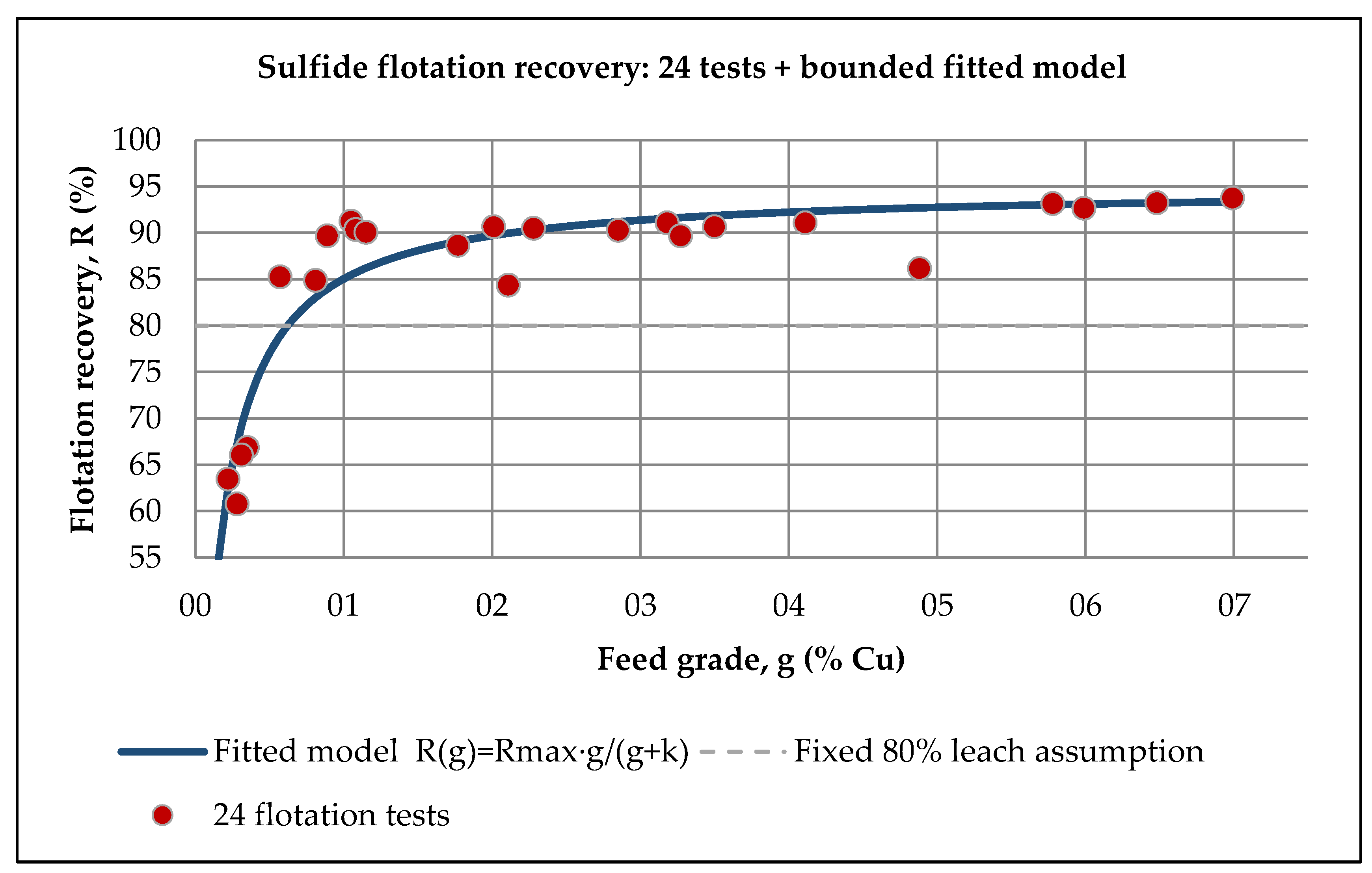
Figure 2.
Block Model (isometric) ≥ 0.2% C.
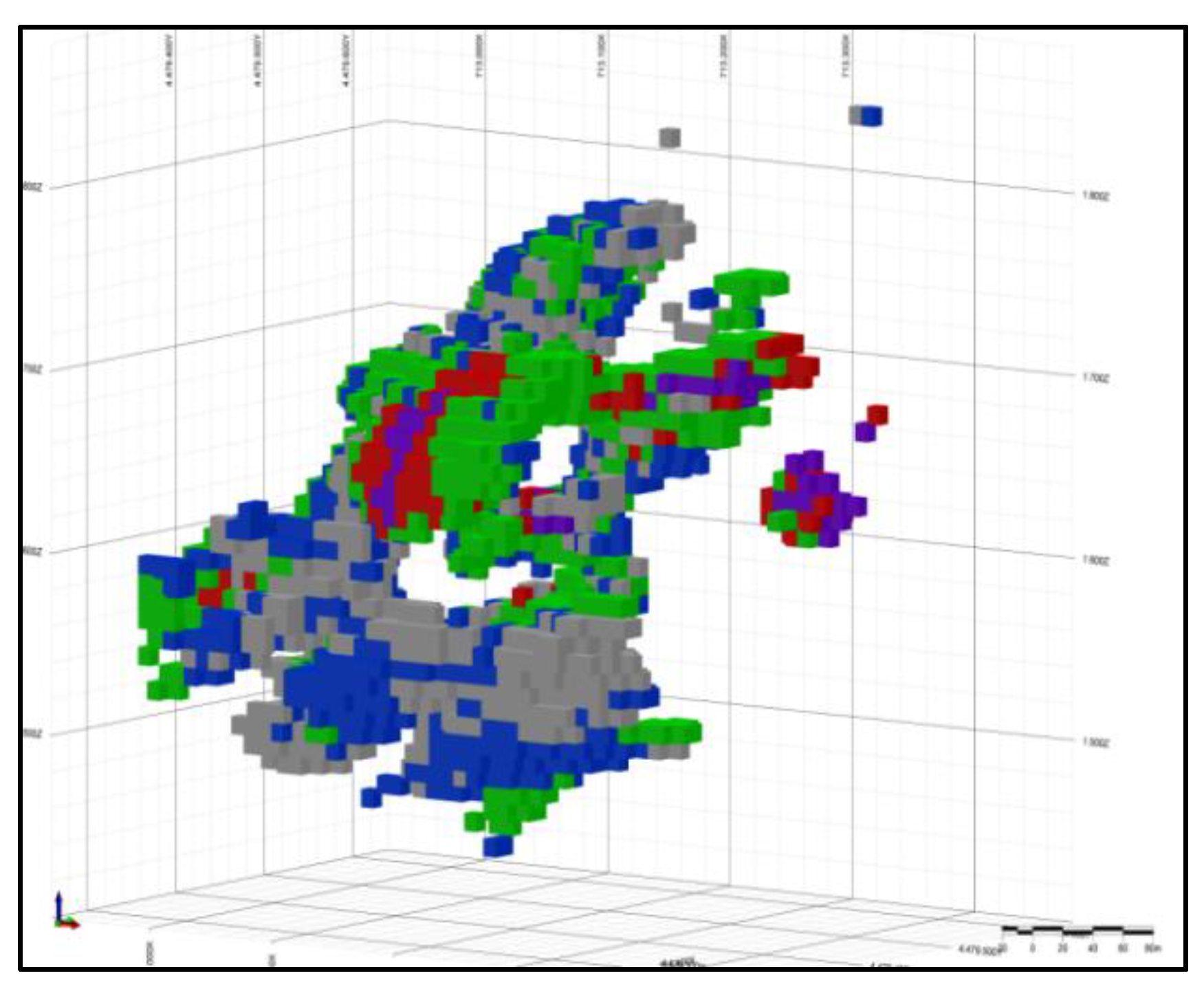
Figure 3.
Block Model Plan View ≥ 0.2% Cu.
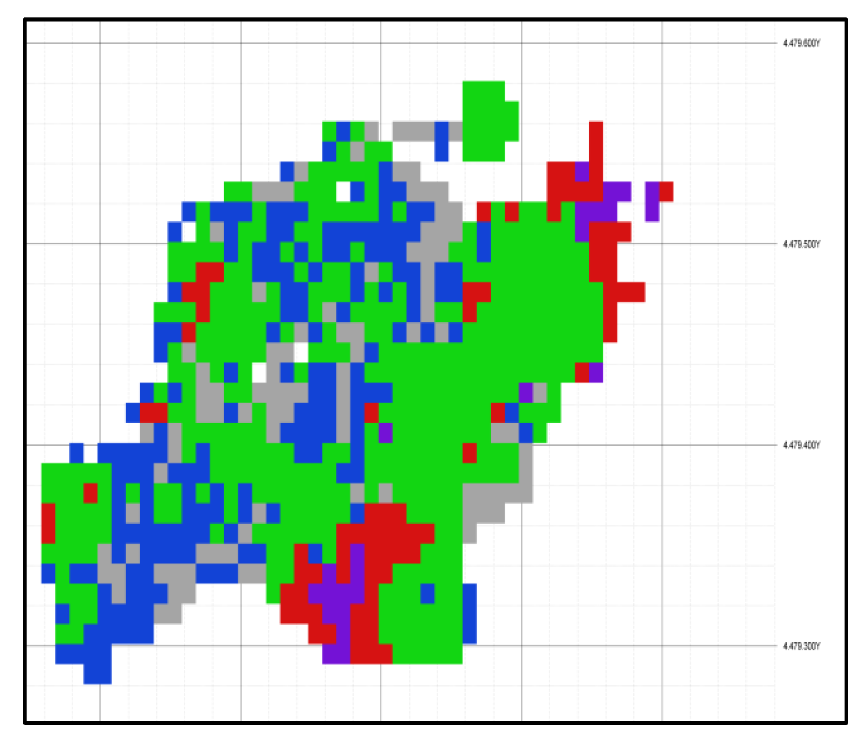
Figure 4.
NPV by scenario under operational and economic cut off.
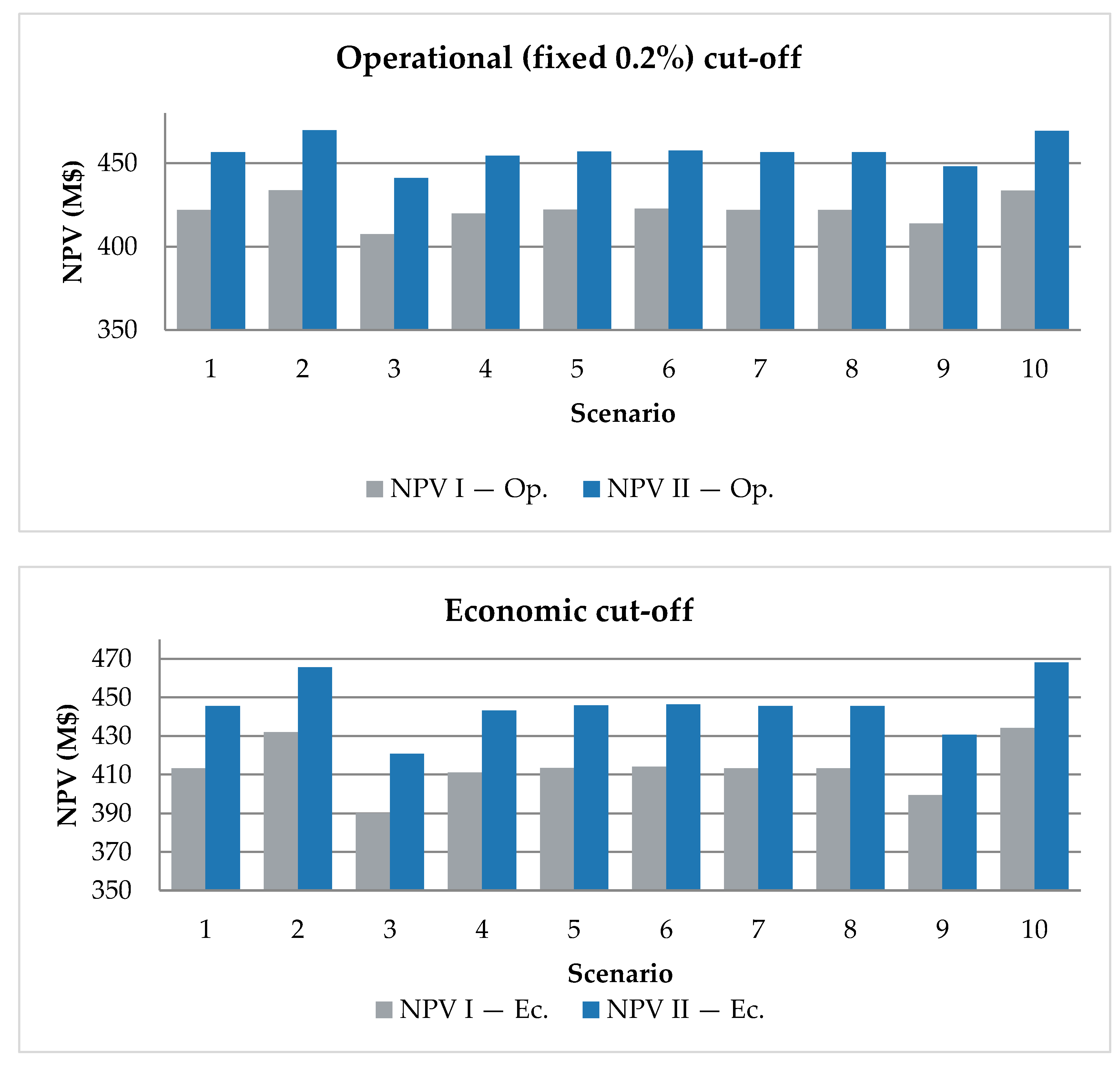
Figure 5.
Ore tonnage and Recovered copper, fixed vs variable recovery (economic cut-off).
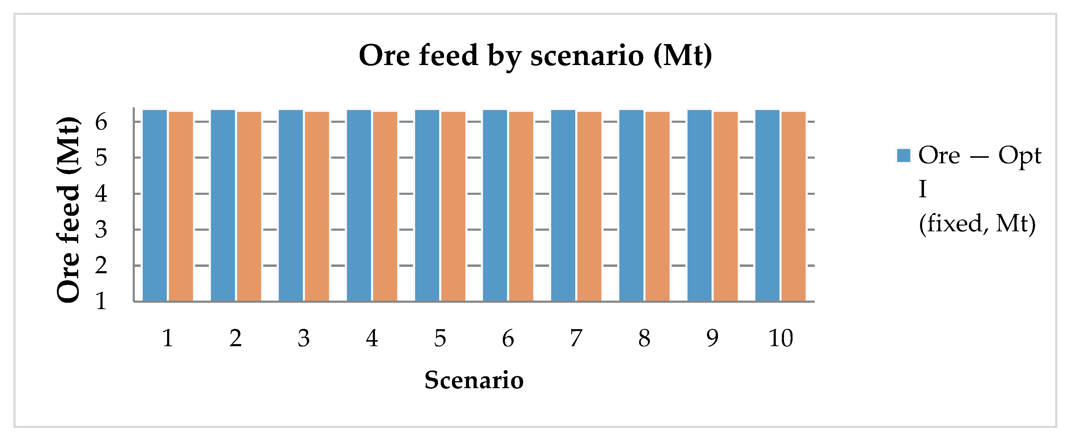
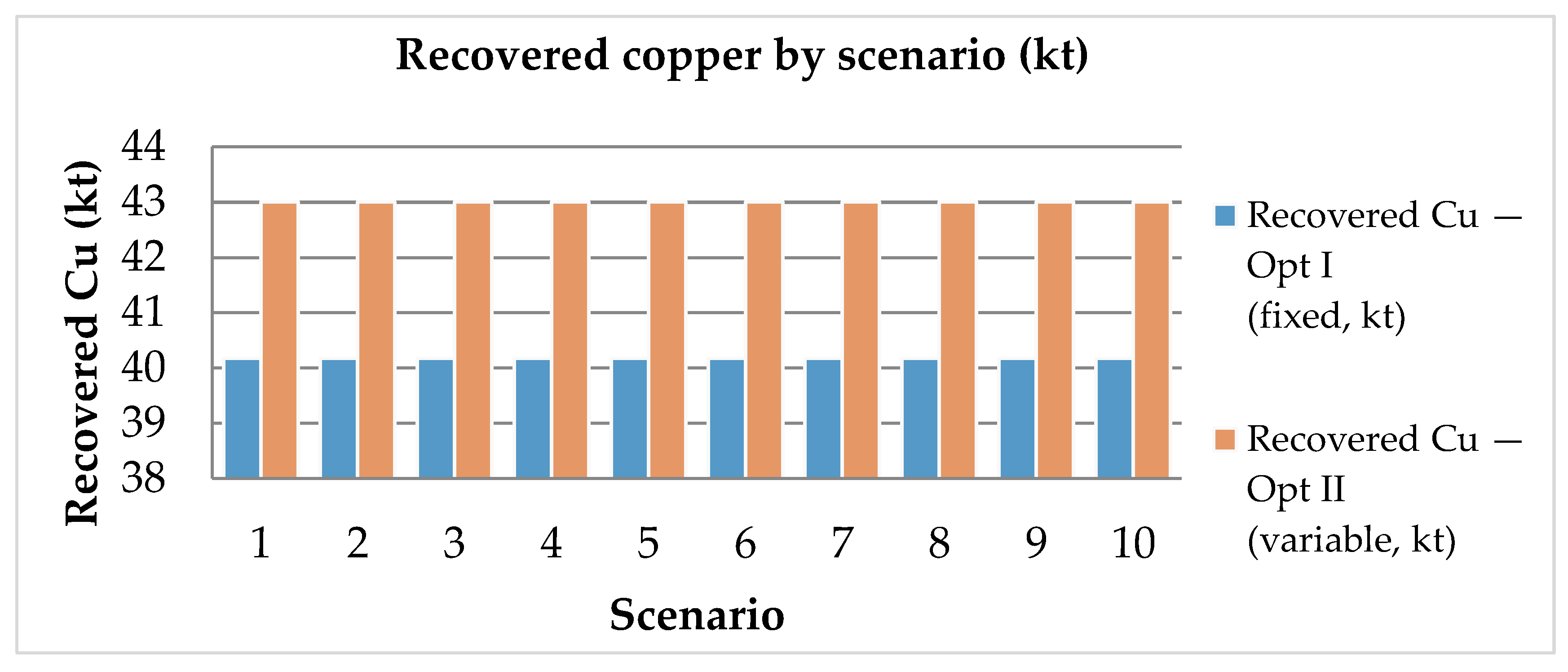
Figure 6.
NPV vs Cu price under fixed and variable recovery.
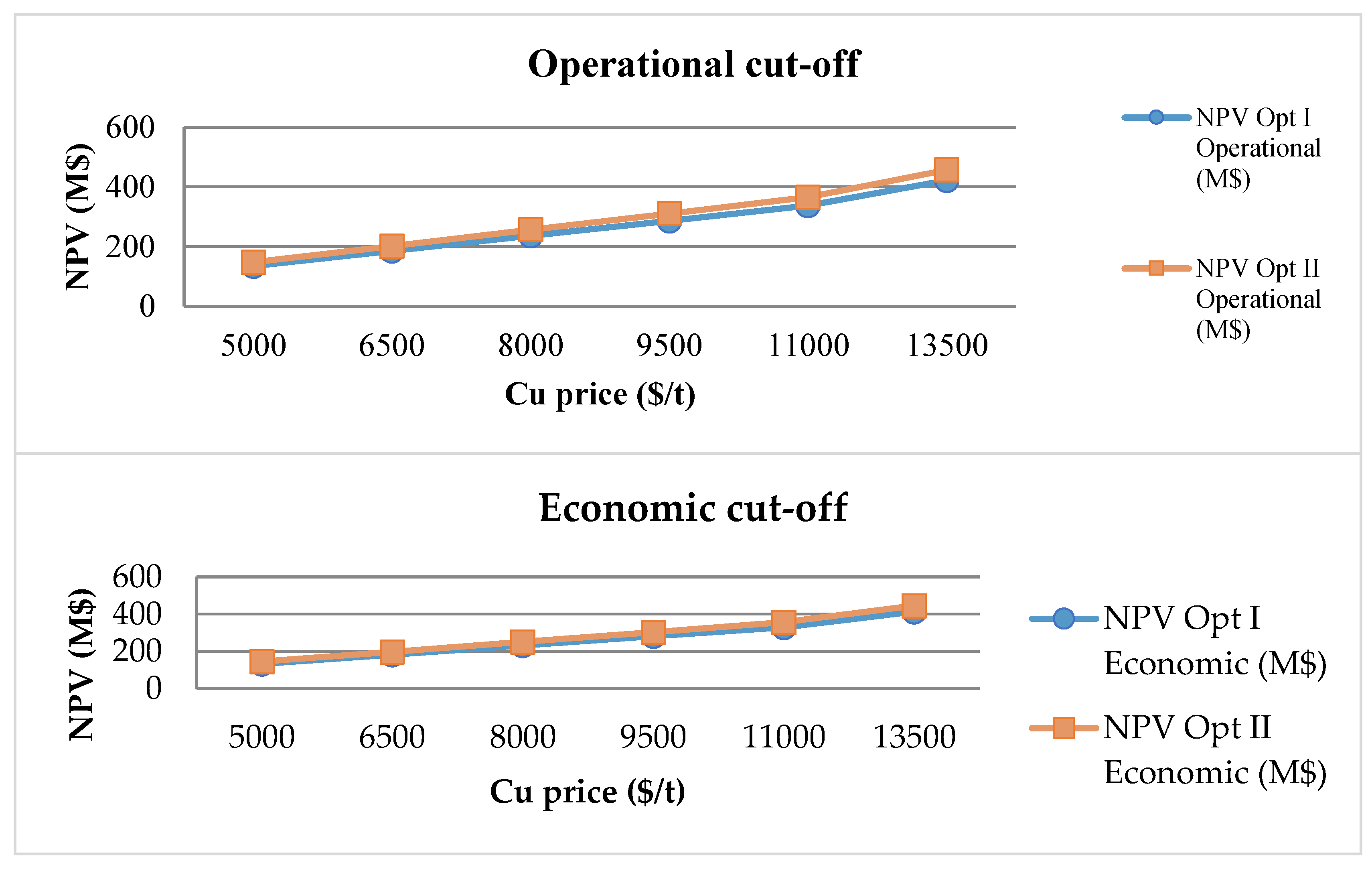
Table 3.
Descriptive statistics of block-model variables.
| Parameter | Min | Max | Mean | St.Dev | 5% | 95% |
|---|---|---|---|---|---|---|
| Cu_% | 0.001 | 7.603 | 0.688 | 0.947 | 0.038 | 2.884 |
| S | 0.000 | 41.002 | 7.254 | 6.086 | 1.031 | 19.528 |
| Density | 2.473 | 4.130 | 2.969 | 0.237 | 2.707 | 3.452 |
Table 8.
Ten optimization scenarios (overall slope 50°, discount 5%).
| Scenario | Flot./Leach capacity (Mt/yr) | Vertical excavation (m/yr) | Mining capacity (Mt/yr) |
|---|---|---|---|
| 1 | 1.0 / 0.5 | 100 | 3 |
| 2 | 1.5 / 0.75 | 100 | 3 |
| 3 | 0.7 / 0.35 | 100 | 3 |
| 4 | 1.0 / 0.5 | 50 | 3 |
| 5 | 1.0 / 0.5 | 150 | 3 |
| 6 | 1.0 / 0.5 | 200 | 3 |
| 7 | 1.0 / 0.5 | 100 | 2 |
| 8 | 1.0 / 0.5 | 100 | 5 |
| 9 | 1.2 / 0.4 | 100 | 3 |
| 10 | 0.8 / 0.8 | 100 | 3 |
Table 9.
Base case results (operational cut-off, 13,500 $/t). NPV in M$, tonnages in Mt, Cu in kt.
| Scn | Ore I (Mt) | Ore II (Mt) | Waste I (Mt) | Waste II (Mt) | NPV I (M$) | NPV II (M$) | Cu I (kt) |
Cu II (kt) | Per I (yr) | Per II (yr) |
|---|---|---|---|---|---|---|---|---|---|---|
| 1 | 4.01 | 4.01 | 1.84 | 1.84 | 422.0 | 456.8 | 37.9 | 40.9 | 4 | 4 |
| 2 | 4.01 | 4.01 | 1.84 | 1.84 | 433.9 | 469.8 | 37.9 | 40.9 | 3 | 3 |
| 3 | 4.01 | 4.01 | 1.84 | 1.84 | 407.6 | 441.3 | 37.9 | 40.9 | 6 | 6 |
| 4 | 4.01 | 4.01 | 1.84 | 1.84 | 419.9 | 454.6 | 37.9 | 40.9 | 6 | 6 |
| 5 | 4.01 | 4.01 | 1.84 | 1.84 | 422.2 | 457.1 | 37.9 | 40.9 | 4 | 4 |
| 6 | 4.01 | 4.01 | 1.84 | 1.84 | 422.8 | 457.7 | 37.9 | 40.9 | 4 | 4 |
| 7 | 4.01 | 4.01 | 1.84 | 1.84 | 422.0 | 456.8 | 37.9 | 40.9 | 4 | 4 |
| 8 | 4.01 | 4.01 | 1.84 | 1.84 | 422.0 | 456.8 | 37.9 | 40.9 | 4 | 4 |
| 9 | 4.01 | 4.01 | 1.84 | 1.84 | 413.9 | 448.1 | 37.9 | 40.9 | 5 | 5 |
| 10 | 4.01 | 4.01 | 1.84 | 1.84 | 433.7 | 469.5 | 37.9 | 40.9 | 3 | 3 |
Table 10.
Economic cut-off results (13,500 $/t).
| Scn | Ore I (Mt) | Ore II (Mt) | Waste I (Mt) | Waste II (Mt) | NPV I (M$) | NPV II (M$) | Cu I (kt) |
Cu II (kt) | Per I (yr) | Per II (yr) |
|---|---|---|---|---|---|---|---|---|---|---|
| 1 | 6.36 | 6.31 | 0.30 | 0.34 | 413.2 | 445.5 | 40.2 | 43.0 | 9 | 9 |
| 2 | 6.36 | 6.31 | 0.30 | 0.34 | 431.9 | 465.6 | 40.2 | 43.0 | 6 | 6 |
| 3 | 6.36 | 6.31 | 0.30 | 0.34 | 390.1 | 420.7 | 40.2 | 43.0 | 12 | 12 |
| 4 | 6.36 | 6.31 | 0.30 | 0.34 | 411.0 | 443.2 | 40.2 | 43.0 | 9 | 9 |
| 5 | 6.36 | 6.31 | 0.30 | 0.34 | 413.4 | 445.8 | 40.2 | 43.0 | 9 | 9 |
| 6 | 6.36 | 6.31 | 0.30 | 0.34 | 414.0 | 446.4 | 40.2 | 43.0 | 9 | 9 |
| 7 | 6.36 | 6.31 | 0.30 | 0.34 | 413.2 | 445.5 | 40.2 | 43.0 | 9 | 9 |
| 8 | 6.36 | 6.31 | 0.30 | 0.34 | 413.2 | 445.5 | 40.2 | 43.0 | 9 | 9 |
| 9 | 6.36 | 6.31 | 0.30 | 0.34 | 399.5 | 430.7 | 40.2 | 43.0 | 11 | 11 |
| 10 | 6.36 | 6.31 | 0.30 | 0.34 | 434.2 | 468.1 | 40.2 | 43.0 | 6 | 6 |
Table 11.
Realized recovery, reclassified ore, and copper difference (economic cut-off).
| Scenario | Fixed R (%) | Variable R (%) | ΔR (pp) | Reclass. ore I−II (Mt) | Cu diff II−I (kt) |
|---|---|---|---|---|---|
| 1 | 80.0 | 85.8 | 5.8 | 0.05 | 2.8 |
| 2 | 80.0 | 85.8 | 5.8 | 0.05 | 2.8 |
| 3 | 80.0 | 85.8 | 5.8 | 0.05 | 2.8 |
| 4 | 80.0 | 85.8 | 5.8 | 0.05 | 2.8 |
| 5 | 80.0 | 85.8 | 5.8 | 0.05 | 2.8 |
| 6 | 80.0 | 85.8 | 5.8 | 0.05 | 2.8 |
| 7 | 80.0 | 85.8 | 5.8 | 0.05 | 2.8 |
| 8 | 80.0 | 85.8 | 5.8 | 0.05 | 2.8 |
| 9 | 80.0 | 85.8 | 5.8 | 0.05 | 2.8 |
| 10 | 80.0 | 85.8 | 5.8 | 0.05 | 2.8 |
Table 12.
Low-price case (9,000 $/t, operational cut-off).
| Scn | Ore I (Mt) | Ore II (Mt) | Waste I (Mt) | Waste II (Mt) | NPV I (M$) | NPV II (M$) | Cu I (kt) |
Cu II (kt) | Per I (yr) | Per II (yr) |
|---|---|---|---|---|---|---|---|---|---|---|
| 1 | 4.01 | 4.00 | 1.79 | 1.79 | 269.6 | 292.7 | 37.9 | 40.8 | 4 | 4 |
| 2 | 4.01 | 4.00 | 1.79 | 1.79 | 277.3 | 301.0 | 37.9 | 40.8 | 3 | 3 |
| 3 | 4.01 | 4.00 | 1.79 | 1.79 | 260.4 | 282.7 | 37.9 | 40.8 | 6 | 6 |
| 4 | 4.01 | 4.00 | 1.79 | 1.79 | 268.3 | 291.3 | 37.9 | 40.8 | 6 | 6 |
| 5 | 4.01 | 4.00 | 1.79 | 1.79 | 269.8 | 292.9 | 37.9 | 40.8 | 4 | 4 |
| 6 | 4.01 | 4.00 | 1.79 | 1.79 | 270.1 | 293.3 | 37.9 | 40.8 | 4 | 4 |
| 7 | 4.01 | 4.00 | 1.79 | 1.79 | 269.6 | 292.7 | 37.9 | 40.8 | 4 | 4 |
| 8 | 4.01 | 4.00 | 1.79 | 1.79 | 269.6 | 292.7 | 37.9 | 40.8 | 4 | 4 |
| 9 | 4.01 | 4.00 | 1.79 | 1.79 | 264.4 | 287.1 | 37.9 | 40.8 | 5 | 5 |
| 10 | 4.01 | 4.00 | 1.79 | 1.79 | 277.1 | 300.9 | 37.9 | 40.8 | 3 | 3 |
Disclaimer/Publisher’s Note: The statements, opinions and data contained in all publications are solely those of the individual author(s) and contributor(s) and not of MDPI and/or the editor(s). MDPI and/or the editor(s) disclaim responsibility for any injury to people or property resulting from any ideas, methods, instructions or products referred to in the content. |
© 2026 by the authors. Licensee MDPI, Basel, Switzerland. This article is an open access article distributed under the terms and conditions of the Creative Commons Attribution (CC BY) license (http://creativecommons.org/licenses/by/4.0/).
Copyright: This open access article is published under a Creative Commons CC BY 4.0 license, which permit the free download, distribution, and reuse, provided that the author and preprint are cited in any reuse.


