

Submitted:
26 June 2026
Posted:
29 June 2026
You are already at the latest version
Abstract
In this paper 31 sediment samples collected from the Danube River, Delta and Black Sea in Romania were investigated by INAA, ICP-MS and CV-AAS techniques for the quantification of 42 elements (Al, Mg, Cl, Ti, Ca, V, Mn, Na, Si, K, Sc, Cr, Fe, Co, Ni, Zn, As, Br, Rb, Sr, Sb, Zr, Mo, Cs, Ba, La, Ce, Sm, Ta, Nd, Eu, Tb, Yb, Lu, Hf, W, Th, U, Cd, Cu, Pb and Hg) and highlighting geochemical peculiarities. Contamination and ecotoxicological risks were evaluated based on single (CF, Er) and complex (PLI, RPLI, RI) indices computed for 26 presumably contaminant elements, suggesting a pollution load in the maritime sector of the Danube and Chilia branch. Significant contribution to the RI had the elements with high toxic response factor, e.g. Hg, rare earth elements (REEs) (Lu having the highest percentage), As, Cd, U, Pb and Sb. Assessment of radiological hazard due to 238U, 232Th and 40K through the absorbed dose rate (ADR), radium equivalent activity index (Raeq), external hazard index (Hex), representative level index (IG), annual effective dose (AED) and excess lifetime cancer risk (ELCR) suggested an elevated radiation exposure of people in the Danube region compared to Black Sea littoral.
Keywords:
sediments
; Danube
; Black Sea
; geochemistry
; INAA
; ICP—MS
; potential contaminant elements
; ecotoxicological risk
; radiological risk
1. Introduction
The second largest river in Europe (2826 km long) and a vital European waterway, the Danube River rises from the Black Forest Mountains (Donaueschingen in Germany), flows into the Black Sea through its three arms—Chilia, Sulina and Sf. Gheorghe—encompassing 19 countries and has been building, for over 12000 years by now, one of the most characteristic and beautiful deltas in Europe through the transport and deposition of sediments [1,2,3,4,5,6,7]. The characteristics and quality of the sediments transported by the Danube reflect human developments over time but, at the same time, the problems related to the environmental state and the socio-economic situation of the river region [2,8,9,10,11].
Sediments could concentrate a large number of waterborne pollutants, including inorganic harmful substances, such as presumably contaminant elements (PCEs)—heavy metals and trace elements, radioelements, rare earth elements (REEs)—which may be released in the surrounding environment, causing habitat degradation and toxicological hazards to aquatic biota and humans consuming them [2,10,11,12,13,14]. The sources of these contaminants in aquatic ecosystems can be of both natural and anthropogenic origin, including erosion processes, base rock weathering, runoffs from agricultural terrains, urbanization, industrialization, effluents resulted from wastewater plants and abattoirs, existence of inadequate waste disposal sites, mineral processing, iron and steel making, harbor activities, shipbuilding, and naval transport [12,15,16,17,18,19]. Instrumental neutron activation analysis (INAA) technique has been extensively used in various studies for multielemental characterization of environmental and biological materials [17,18,20,21,22,23,24,25,26], determination of PCEs and elements of geological interest, with a significant role in soil/sediment mineralogy and provenance studies [14,17,23,24,27,28]. Due to its drawbacks in quantification of several heavy metals of environmental concern (e.g., Cu, Pb, Cd, Hg), INAA can be complemented with other analytical techniques [11], such as Inductively Coupled Plasma Mass Spectrometry (ICP–MS) [10,12,17,21,29] or Atomic Absorption Spectrometry (AAS) [15,21,30].
Several studies have been focused on the monitoring of a limited number of heavy metals and trace elements in the Danube River sediments [10,12,31], including the lower sector in Romania, but in the connected river-delta-sea area was insufficiently investigated as regards the sediment multielement composition [20]. The present work is an extension and completion of regional studies of various classes of inorganic toxicants in the Black Sea Basin and Lower Danube Basin environments (sediments, surface water, soils, water suspensions) [9,10,11,13,17,18,19] performed in the frame of the BSB27 (MONITOX) project (https://www.monitox.ugal.ro/)—a cross-border environmental initiative (2018–2021) funded by the Joint Operational Programme Black Sea Basin 2014-2020 of EU (https://keep.eu/projects/22488/Black-Sea-Basin-interdiscip-EN/) [32].
The aim of this paper is: a) the study of the spatial distribution pattern and geochemistry of 42 major and trace elements in Danube River—Delta—Black Sea sediments; and b) ecotoxicological and radiological risk assessment of selected PCEs in the investigated sediments.
2. Materials and Methods
2.1. Sampling and Sample Processing
Sediment samples were collected from 31 representative points of MONITOX network in the Danube River Basin and Black Sea coast of Romania (Figure 1) [9,10], during the fluvial and marine expeditions organized in June-July 2019 by the MONITOX project teams of Danube Delta National Institute for Research and Development, Tulcea (DDNI), and Dunarea de Jos University of Galati (UDJG), Romania. The sites’ coordinates and description are given in Table 1.
The sediment samples were collected using a Van Veen grab sampler (40 × 40 cm) to minimize disturbance, targeting the upper 5 cm of the sediment layer. This superficial layer was selected due to its higher chemical activity compared to deeper layers, as it represents the primary zone of exchange between sediment and water. The samples were taken from the Danube navigable channel area and from the Black Sea coastal area at a distance of 15–25 m from the shoreline, at depth of about 1.5 m. The collected samples were prepared for various analyses at DDNI and INPOLDE research center of UDJG, dried at room temperature, then grounded and sieved to a granulation of 0.01 mm.
2.2. INAA Analytical Technique
The elemental composition of the samples was determined using instrumental neutron activation analysis (INAA) at the Regata facility of the IBR-2 reactor (Frank Laboratory of Neutron Physics (FLNP), Joint Institute for Nuclear Research (JINR), Dubna) [17,18,35,36]. Before analysis, the sediment samples were dried to constant weight, homogenized, and packed in polyethylene bags or aluminum foil, depending on the type of irradiation.
The content of elements producing short-lived radionuclides (Al, Mg, Cl, Ti, Ca, V, and Mn) was determined by irradiating samples for 3 minutes at a thermal neutron flux of 1.2 × 10¹² n cm–2 s–1, followed by a 15-minute measurement. For elements forming long-lived isotopes (Na, Si, K, Sc, Cr, Fe, Co, Ni, Zn, As, Br, Rb, Sr, Sb, Zr, Mo, Cs, Ba, La, Ce, Sm, Ta, Nd, Eu, Tb, Yb, Lu, Hf, W, Th, and U), the cadmium-screened Channel 1 was used. Samples were irradiated for 4 days at a neutron flux of 1.1 × 1011 cm-2 s-1. Gamma spectra of induced activity were acquired after 4 and 22 days, respectively, using Canberra HPGe detectors with an efficiency of 100% and resolution of 1.8-2.0 keV at 1332 keV 60Co total-absorption peak. Spectral analysis was performed using Canberra’s Genie2000 software, while element concentrations in the samples were calculated using software developed at JINR [35,36].
A set of reference materials (SRM), including NIST 2709a—San Joaquin Soil, NIST 2709 -San Joaquin Soil, NIST 1515- apple leaves, NIST 1547—peach Leaves, NIST 2710 -Montana Soil, NIST 1633b—bituminous coal fly ash, NIST 2711a—Montana II Soil, BCR-667 Estuarine Sediment, CTA-FFA-1- fine fly ash, were irradiated with samples to create group standard and to ensure the quality control of the results. All measurements were performed in triplicate. The quality control results of INAA (elemental determined and certified amounts and respective uncertainties) along with minimal detectable concentrations (MDC) is given in Table 2.
2.3. ICP-MS and CV-AAS Techniques
The extraction of the four selected metals (Cd, Hg, Pb, Cu) from sediment samples was performed according to EPA Method SW-846 3051A (2007): Microwave-Assisted Acid Digestion of Sediments, Sludges, Soils, and Oils [37].
For mineralization, a 20 g subsample was air-dried to prevent mercury loss. For the determination of Cd, Hg, Pb, and Cu, a 0.1 g sediment subsample was digested with 10 mL of concentrated HNO3 for 20 minutes using an Anton Paar Multiwave 3000 microwave digestion system. Digestion was carried out in quartz tubes (XQ80-8 rotor) at a pressure of 7.5 ± 0.7 atm. The operating program consisted of 600 W for 5.5 minutes, followed by 1200 W for 4.5 minutes. After cooling to room temperature, the digest was quantitatively transferred into 100 mL volumetric flasks and diluted to volume with ultrapure water.
Mercury concentrations were determined by cold vapor atomic absorbtion spectrometry (CV-AAS) using a FIMS400 spectrometer based on flow injection mercury hydride atomic absorption spectrometry (FI-MH-AAS), employing a reducing agent (0.2% NaBH4 in 0.05% NaOH), transport solution (3% HCl), and oxidizing solution (5% KMnO4), in accordance with SW-846 Method 7000A [38] and Method 7471B [39] (Mercury in Solid or Semisolid Waste—Manual Cold-Vapor Technique).
Quantitative determination of Cd, Pb, and Cu was carried out by ICP-MS (Elan DRC-e), following EPA Method SW-846 6020 B (Inductively Coupled Plasma—Mass Spectrometry) [40], with measurements performed in triplicate.
For mercury, the calibration curve was drawn with Merck, Certified Reference Material 1000 mg/L Mercury in 5% HNO3, Lot HC 7265526, by successive dilutions, to concentrations of 1 µg L-1, 2 µg L-1, 4 µg L-1, 6 µg L-1, 8 µg L-1, 10 µg L-1 (the regression coefficient of the curve was 0.997) and for the other three metals, namely cadmium, mercury and lead, with MRC ICP multielement calibration Standard VI (No Hg) Merck, Lot HC15473080, stock of 10 mg mL-1, in the concentration range: 2 µg L-1, 4 µg L-1, 6 µg L-1, 8 µg L-1, 10 µg L-1 (regression coefficients were 0.998, 0.999 and 0.996, respectively).
Analytical quality control was achieved using the certified reference material for metals in Soil, Sigma-Aldrich, Product Id SQC001-30g Lot LRAC3749 (Cd 149±6 mg kg-1, Hg 14±1 mg kg-1, Pb 333±13 mg kg-1, Cu 225±9 mg kg-1). The recovery percentages (%) of Cd, Hg, Pb, Cu concentrations from the reference material were 98.14, 97.24, 98.21 and 99.12, respectively. The quantification limits were 0.2 µg kg-1 for Cd, Pb, Cu, and 0.1 µg kg-1for Hg. The detection limits were 0.1 µg kg-1 for Cd, Pb, Cu, and is 0.05 µg kg-1 for Hg.
2.4. Contamination and Ecotoxicological Risk Indices
In order to describe the pollution degree and ecotoxicological risk in a target area impacted by multi-pollutants, several single and complex (multielement) contamination [41,42] and ecological risk [42] indices (Table 3) have been extensively used to evaluate the impact of selected PCEs on the sediment quality and surrounding aquatic ecosystem state, such as: Contamination Factor—CF (Equation (1)), Pollution Load Index—PLI (Equation (2)), Regional Pollution Load Index —RPLI (Equation (3)), Ecological risk factor— (Equation (4), and Potential Ecological Risk Index—RI (Equation (5)) [17,18,43].
For the toxic-response factors the following values established by Hakansson [41] for the heavy metals Hg, Cd, As, Pb, Cu, Cr and Zn, or reported/used in various studies [17,44,45,46,47,48,49,50,51,52,53] for Co, Ni, Mn, rare earth elements (REEs), W, U, V, Sb, Ba, Mo, Fe and Ti have been used in calculation of the Ecological risk factor () for the selected trace elements (n=26) with documented toxicity for the aquatic ecosystems: Hg–40 [41], Cd–30 [41], As–10 [41], Pb–5 [41], Cu–5 [41], Co–5 [17], Ni–5 [17], Cr–2 [41], Mn–1 [17], Zn–1 [41], REEs (La–1, Ce–1, Nd–2, Sm–5, Eu–10, Tb–10, Yb–5, Lu–20) [44], W–2 [45], U–40 [46], V–2 [47], Sb–7 [48,49], Ba–2 [50], Mo–18 [51], Fe–1 [52], Ti–1 [53].
For the calculation of CFs, the Upper Continental Crust (UCC) values specified in [54] have been used.
2.5. Radiological Parameters
To assess the radiological and human health risk of sediments’ radioactivity, we computed the absorbed gamma dose rate (ADR) due to natural radionuclides and the associated radiological parameters − radium equivalent activity index (Raeq), external hazard index (Hex), representative level index (IG), annual effective dose (AED), and excess lifetime cancer risk (ELCR) − reported in other studies [19,55,56,57,58].
ADR (nGy⋅h−1) in air at 1 m above ground due to the natural radionuclides in sediment was calculated from the activity concentrations A(U), A(Th) and A(K) (in Bq⋅kg−1) of 238U, 232Th and 40K, respectively, with the aid of Equation (6):
where the values of 0.462, 0.604 and 0.0417, expressed in nGy⋅h−1 per Bq⋅kg−1, represent the activity to-outdoor dose conversion factors for the natural radionuclides. In Equation (6), the activity concentrations of 238U, 232Th and 40K were calculated using the results provided by INAA technique for the mass fractions of the radioelements U, Th and K, respectively [25,58,59], considering that 1 g natural U yields 12357 Bq 238U, 1 g natural Th yields 4069 Bq 232Th, and 1 g K yields 31.66 Bq 40K [19].
ADR (nGy⋅h−1) = 0.462 A(U) + 0.604 A(Th) + 0.0417 A(K)
With the notations given above, the radiological parameters have been assessed using the following equations (Equations (7)–(11)) [19,55,56,57,58]:
Raeq (Bq⋅kg−1) = A(U) + 1.43 A(Th) + 0.077 A(K)
Hex = A(U)/(370 Bq⋅kg−1) + A(Th)/(259 Bq⋅kg−1) + A(K)/(4810 Bq⋅kg−1)
IG = A(U)/(150 Bq⋅kg−1) + A(Th)/(100 Bq⋅kg−1) + A(K)/(1500 Bq⋅kg−1)
AED (mSv⋅y−1) = DR (nGy⋅h−1) ⋅ 8760 h⋅y−1 ⋅ 0.2 ⋅ 0.7 Sv⋅Gy−1 ⋅ 10−6
ELCR = AED (mSv⋅y−1) ⋅ 70 y ⋅ 0.055 Sv−1 ⋅ 10−3
2.6. Statistical Data Analysis and Mapping
All statistical analyses were performed by means of the PAST freeware (https://www.nhm.uio.no/english/research/resources/past/) [60,61] as well as OriginLab® Origin 10 software (https://www.originlab.com/origin) [62], and MS Excel 2019.
All data concerning the distribution of Pollution Load Index (PLI) were processed by the Spatial Analyst specific tools provided by ArcMap 10.4 [https://desktop.arcgis.com/en/arcmap/latest/analyze/main/what-is-geoprocessing.htm] [63]. This permitted to obtain a qualitative picture of the PLI spatial distributions along the low-water channel of the investigated Danube River sector. The experimental data were interpolated using the Inverse Distance Weighting (IDW) technique with a cell size of 100. The resulted map was represented using the Lambert azimuthal projection. This was done by means of the Surface volume tool in 3D Analyst of the same ArcMap 10.4 software.
3. Results and Discussion
3.1. Geochemistry of Sediments from Danube River-Danube Delta-Black Sea System
3.1.1. Spatial Distribution of Elements in Sediments
The results obtained for elemental mass fractions by employing the combined analytical methods INAA, ICP-MS and CV-AAS highlighted the existence of 42 elements in sediments, whose mass fractions (in mg·kg-1) are given in Table S1 (Supplementary Materials), together with descriptive statistics parameters (minimum—min; maximum—max; average—ave; standard deviation—SD; median—med) and coefficients of variations (CV) and literature data for element content in stream sediments [64]. Chlorine was only detected in 3 sites from the Black Sea. Figure 2 shows the spatial distribution of the elemental amounts.
Comparison of the major element concentrations with the European median stream baseline values [64] revealed sediment enrichment primarily in Mn, Ca, and Na. Based on the number of elements exceeding the reference values (out of 9 analyzed major elements), site 8 did not show any exceedances, whereas site 21 recorded five exceedances, involving Ti, Mn, Mg, Ca, and Na.
Comparison with the European median stream baseline values [64] revealed elevated concentrations of several PCE—trace elements across the study area. Mercury (Hg) was the only element whose concentrations exceeded the reference value at all studied locations. Other elements that showed exceedances at most sampling sites were lead (Pb), nickel (Ni), and chromium (Cr). Considering the number of elements (out of 23) that exceeded the reference values [64], site 1 exhibited the fewest number of exceedances, with only Hg, Ni, and Pb exceeding the baseline levels. In contrast, site 18 showed the highest number of exceedances (21 out of 23 elements), with only Ba and Cd remaining below the European median stream reference values [64].
For other trace elements, not included in the PCE group, such as Sr, Hf, Ta, Th, and Zr, higher values of mass fraction were found, compared with European median stream reference values [64]. No reference values were available for Br and Sc; therefore, these elements could not be evaluated in terms of exceedance. The fewest exceedances were observed for Cs and Th. The highest Cs concentration was recorded at Site 12 (5.65 mg kg−1), whereas the highest Th concentration was measured at Site 7 (18.5 mg kg−1). Strontium (Sr) was one of the most frequently enriched elements, with concentrations exceeding the Salminen reference value at the majority of sampling sites. The maximum concentration was recorded at Braila harbor downstream (Site 7), reaching 165 mg kg−1.
Taking into account the chemical quality standards for sediments (<63 μm fraction) established by the Order no. 161/2006 [65], all measured values of As, Cd, Pb, and Zn were lower than the corresponding standard values of 29, 0.8, 85, and 150 mg kg−1, respectively. However, elements such as Cr, Cu, Hg, and Ni presented values higher than those established by the legislation [65]. Cr exceeded the limit value of 100 mg kg−1 [65] at seven locations (7, 10, 11, 13, 17, 18, and 19), with concentrations ranging between 100 and 440 mg kg−1. Cu exceeded the legal limit at only five locations (11, 12, 19, 20, and 22), with concentrations ranging from 40.5 to 51.2 mg kg−1. Hg amount was above the legal limit of 0.3 mg kg−1 [65] only at locations 29 and 30, with values of 0.34 and 0.35 mg kg−1, respectively. Ni was another element that presented concentrations above the legal limit of 35 mg kg−1 [65] at locations 10, 12, 17, 19, 20, 21, and 24, with concentrations ranging between 36 and 50 mg kg−1.
Compared to 1996 study [20], the 2019 sediment samples generally presented higher maximum and average concentrations for most of the analyzed elements (Figure 3 and Figure 4). The most notable differences can be observed for Ti and Mn. In the case of Ti, the maximum concentration recorded in 1996 (40 mg kg−1) [20] was 5.35 times lower than the maximum value determined in 2019 (214 mg kg−1). Mn, on the other hand, exhibited a maximum concentration of 339 mg kg−1 in 2019, which was 2.44 times higher than the value recorded in 1996 (139 mg kg−1) [20]. In contrast, Si presented relatively stable concentrations.
3.1.2. Major Elements in Sediments
The mass fractions of all nine major, rock forming elements which corresponds to the Danube River fluvial sediments are provided in Table A1 (Appendix A), while those corresponding to the Black Sea marine sediments are reproduced in Table A2 (Appendix A). In both cases, the mass fractions are expressed in percent of corresponding oxides. Also, the values for UCC [54], NASC [66], Average World Suspended Sediments (AWSS) and [67], Dobrogea Loess (DL) [68] are presented in Table A1 and Table A2.
The data reproduced in Table A1 shows that silicon represents the dominant element, followed by aluminum and calcium. The mass fractions of the other elements (as oxides) follow the following order: Mg > Fe > > Na > K > Ti > Mn, very similar as the UCC, NASC, AWSS and even DL. All these data pointed a common, continental origin of the depositional material of the analyzed Danube River sediments.
Also, the corresponding distribution functions of the same data normalized to the UCC [54] are illustrated in Figure 5. Accordingly, although for almost all elements, there were small discrepancies between average and median, their mass fractions were close to the UCC one, suggesting a continental origin of the deposition material. Excepting three outliers, i. e. TiO2, MnO and CaO, the distribution of the mass fractions of all other elements appeared uni-modal, suggesting a relative uniformity of their distribution (Figure 5a).
Further, the analysis of the corresponding tree diagram (Figure 5b) evidenced two main clusters, well separated, one of them consisting only of SiO2. The most likely explanation of this finding points towards quartz as the main component of sediments. It is of interest to remark the fact that SiO2 and TiO2 form another small cluster, while the other elements form another small cluster, almost indistinguishable, which suggests a relative uniformity of the nature of the sedimentary material. More details on the sediments’ nature is provided by the log(Na2O\K2O) vs. log (SiO2\Al2O3) bi-plot [69] (Figure 5c) and by the Na2O/Al2O3 vs. K2O/Al2O3 one [70] (Figure 5d). While the log(Na2O\K2O) vs. log (SiO2\Al2O3) bi-plot suggests a lith-arenitic origin of sediments, the log(Na2O\K2O) vs. log (SiO2\Al2O3) one allows classification of the investigated sediments in the “Flood plain” category, in good correlation with the fact that the Danube River crosses both the Pannonian [23] and Romanian plains.
On contrary, the distribution of the same elements in the marine sediments, illustrates quite different situation (Figure 6 and Table A2, Appendix A). In this case, although silicon continues to be the dominant element, its mass fraction as oxide is smaller than those reported for all reference systems, e.g., UCC, NASC, AWSS and DL. The same peculiarity characterizes almost all other elements excepting calcium, of which mass fraction as CaO overpasses the references one by about one order of magnitude. Moreover, the mass fraction all major elements presents a significant variability varying between 31% in the case of sodium oxide and about 160% in the case of titanium oxide.While the increased variability can be partially attributed to the reduced number of sampling points spread on almost Black Sea Romanian shore, as the distance between Gura Portitei and Mangalia is about 125 km, corresponding to a sampling rate of 1 sample/25 km. On the other hand, the relatively reduced presence of the majority of major elements mass fractions accompanied by a significant increase in calcium one can be attributed to a significant fraction of marine bivalves and gastropods shell debris, as well as possible Emiliania huxleyi Lohmann calcareous coccoliths [27,71].
But, given the evidenced variability on one hand and the increased presence of Ca, on the other, the geochemistry of the Black Sea shallow zone sediments deserves more interest, so the presented data could be considered as a modest attempt.
3.1.3. Trace Elements in Sediments
Another main advantage of the INAA consists in its ability to determine in the same time the mass fractions of about 30 trace elements, allowing a better description and understanding of the geochemical peculiarities of the chosen system.
In the case of the present study, INAA allowed determining the mass fraction of 30 elements, the majority belonging to the class of incompatible elements [72] which acts as tracers in petrology allowing to infer the nature and provenience of a large category of rocks and minerals, including the sedimentary ones.
Accordingly, the mass fractions of the following elements were determined with a total uncertainty of about 8-10%, i.e., Sc, V, Cr, Co, Ni, Zn, As, Br, Rb, Sr, Zr, Mo, Sb, Cs, Ba, La, Ce, Nd, Sm, Eu, Tb, Yb, Lu, Hf, Ta, W, Th, and U. To complete our study concerning the anthropogenic contamination of the Danube River sediments, the mass fractions of another four Presumably Contaminating Elements (PCEs), i.e., Cu, Cd, Hg, and Pb were determined by ICP-MS and CV-AAS, given the INAA’s inadequacy to dose these elements (Table A3, Appendix A). Although their majority consists of incompatible or even High Field Strength Elements (HFSEs), certain of them such as V, Cr, Co, Ni, Cu, Zn, As, Sb, Cd, Hg and Pb belong to the PCEs group, and therefore they are discussed separately.
For a unitary presentation, the mass fractions of all investigated trace elements were normalized to the UCC [54] (Figure 7). Accordingly, Figure 7a is devoted to all incompatible and HSF elements other than PCE ones, while Figure 7b concerns all investigated PCEs, regardless their mass fractions were determined by INAA or ICP-MS and CV-AAS.
Concerning the first category of elements, the data illustrated in Figure 7a) points towards a relative closeness to the UCC [54] values, while in the case of PCE elements, only Hg and Pb showed values of which mass fraction exceeded the UCC ones by a factor up to 4, as the case of Hg. In the case of all PCE, it worth mentioning that the UCC mass fractions were considered as reference when the Contamination Factors (CF) were calculated (see the next subsection), which situated this report in a more conservative treatment, as UCC can be considered as the best approximation of pristine, uncontaminated environment.
As mentioned before, the presence of incompatible and HFSEs, permits inferring valuable information concerning not only the origin of sedimentary material but also the influences of environmental factors during their transport and position.
Accordingly, Rb/Sr ratio is a widely used geochemical marker to evaluate the extent of chemical weathering in soils and sediments [73]. In the case of investigated sediments, this ratio was of 0.37 ± 0.13, comparable with experimental uncertainty with those of the UCC of 0.26 [54], NASC of 0.71 [66], Average World Suspended Sediments (AWSS) of 0.42 and [67], or 0.35 in the case of Dobrogea Loess (DL) [68], which suggests a low intensity of weathering, which can be attributed to a relatively young age of the sediments transported by the Danube River.
At their turn, the incompatible V and Ni, together with the HFSE Sc, La and Th were intensively used in evidencing the nature of a large category of rocks. In the present case, two discriminating ternary diagrams, e.g., Sc-La-Th [74], and V-Ni-10*Th [75], proved the belonging of considered sediments to the clay, silt and gravels from mixed sources varieties (Figure 8a) as well as to the felsic category of rocks (Figure 8b). In this regard, it is worth mentioning that a similar behavior was noticed for the UCC, NASC, WASS and DL sedimentary materials. This finding was confirmed by the discriminating bi-plot La/Th vs. Hf [70], all elements belonging to HFSE group, where all data points are grouped in the region of felsic source. Only some samples showed the presence of old sedimentary material, similar to the DL (Figure 8c), confirming the previous remark concerning their felsic origin.
Further, another discriminating bi-plot—Th/Sc vs. Zr/Sc [76] showed a grouping of experimental point around UCC, NASC and AWSS, and only few of them, enriched in Zr confirmed the previous finding concerning the presence of some recycled material (Figure 8d). In this regard it should be remarked that Zr and Hf have the same behavior, so that the presence of a certain sediment recycling (Figure 8d) is consistent with the previous remark concerning the presence of old sedimentary components.
Both Zr and Hf belong to the 4th group of transition elements, presenting the most similar chemical properties of any elemental pair in the periodic table of elements. For this reason, the Zr/Hf mass fractions ratio is an excellent index for the homogeneity of magmatic rocks which during weathering generate the sedimentary material. In the case of investigated sediments, the Zr/Hf ratio of 36.42 ± 1.14, as well as the correlation factors of 0.998 (Pearson) and 0.985 (Spearman) (Figure 8e), proved the homogeneity of the source rock as well as their felsic origin.
The Lanthanides form a group 15 HFS elements from La (Z=57) to Lu (Z=71) with very similar chemical properties and whose distribution is currently used in inferring data on the nature and evolution of a large category of minerals and rocks [80]. In this regard, the La/Th ratio is a good proxy of the sedimentary material origin [77], as a ratio around 2.9-3.1 confirm a continental origin, which is well evidenced by the Th vs. La, of which ratio 3.1 ± 0.15 fits perfectly this value (Figure 8f).
Moreover, the relative distribution to some REE with respect to the UCC [54] (Figure 7a), showed slightly lower mass fractions for all investigated Lanthanides, with the exception of Yb and Lu, of which mass fractions slightly exceeded the UCC one. This finding is well illustrated by the La vs. Lu biplot (Figure 8g), which evidenced for the La/Lu a ratio of 51.3 ± 5.4, quite different from the value of 100 reported for the UCC [54], 106.7 for AWSS [67], and 80 for DL [68], but closer to the NASC value of 68.2 [66].
On this point it worth mentioning that, in the case of unconsolidated sediments of which material comes from many disseminated sources belonging to different formations, the UCC represents the best reference. At the same time, as INAA is able to determines the mass fractions of only eight Lanthanides, the date provided in Figure 8h was restrained only to La, Ce, Nd, Sm, Eu, Th, Yb and Lu. Despite it, by comparing their distribution with the similar distribution in NASC [66], WASS [67] or DL [68], evidences significant differences, covered by the relatively higher experimental uncertainties (Figure 8h).
Finally, the Th/U is useful in provenance study as a Th/U ratio greater than 0.5 indicate an igneous origin while if the ratio is lower than this threshold, this points toward a metamorphic origin [78,81]. The value found in the present study of 3.43 ± 0.15, is in good concordance with the same ratio reported for UCC [54] of 3.89, 3.67 reported for the AWSS [67] and 3.74 in the case of average DL [68] and even 4.59 in the case of NASC [66], and suggests an igneous origin of the sedimentary material, in good correlation with the above mentioned observations.
In the case of trace elements distribution in the Black Sea sediments, some peculiarities could be remarked. This concerns both incompatible and HFSE (a) and PCE (b) elements as in can be remarked in Figure 9, the absolute majority of elements presented mass fractions lower than the corresponding UCC [54], with the exception of Sr, Br and Hg.
In the case of Sr this peculiarity can be well explained by taking into account the increased presence of CaO, as Sr belonging to the second group of alkali-earth elements as Ca, substitutes for it in marine bivalves of calcareous exoskeleton, on major component of the investigated Black Sea sediments. At its turn, the increased presence of Br in marine sediments can be explained by its connection with the carbon cycle, as Br frequently bonds with the organic carbon [82].
Concerning PCE, it can be remark quasi-absence of all of them, their mass fraction being lower than the UCC [54] excepting the Hg, of which the Contamination Factor reported to the UCC [54] reached a value of 0.25 ± 0.08 mg/kg, which exceeds five-fold the reference value of 0.05 mg/kg [54]. It is worth mentioning that the maximum values of 0.34, 0.35 and 0.28 mg/kg were reached at Constanta, Costinesti and Mangalia respectively, all of them being important tourist resorts.
3.2. Risk assessment of Harmful Elements in Danube-Black Sea Sediments
3.2.1. Contamination and Ecotoxicological Risk Assessment
Individual contamination factors CF were calculated firstly for n=14 presumably contaminant elements (PCEs) (Hg, Cd, As, Pb, Cu, Co, Ni, Cr, Mn, Zn, Ba, Mo, V and Sb) and secondly for another 12 PCEs (metals, trace elements, radioelements, rare earth elements) with documented toxicity for aquatic life (Fe, Ti, W, U, La, Ce, Nd, Sm, Eu, Tb, Yb, Lu) and the results are presented in Table B1 (Appendix B).
In general, the contamination factor (CF) was smaller than 1 for most of the analyzed elements, indicating a low level of pollution.
Mercury (Hg) exhibited the highest CF values. Except for locations 1, 2, 4, 5, 14, and 27, where the CF indicated moderate contamination, and locations 28 and 30, where the CF corresponded to a very high level of pollution, all remaining locations showed considerable contamination.
In addition to Hg, only Ti at location 27 and As at location 5 indicated a very high level of pollution according to the CF values.
At location 7, several elements showed a considerable level of contamination, as: Cr, Hg, Lu, Mn, Ti, and Yb.
The spatial distribution of PLI values computed for selected n=14 PCEs, e.g., Hg, Cd, As, Pb, Cu, Co, Ni, Cr, Mn, Zn, Ba, Mo, V and Sb, for m=31 investigated sites, is drawn in Figure 10. The experimental data concerning the spatial distribution of PLI values for selected PCEs were organized in a geospatial data base, further processed by ArcMap 10.4 Spatial Analyst [63], which permitted to generate a map representing the spatial distribution of site PLI indices (Figure 10).
For the more in-depth evaluation of the site pollution risk, the PLI was also calculated for the larger group of harmful elements, totaling n=26 PCEs. The comparison of PLI-14 and PLI-26 levels is presented in the Figure 11, evidencing the lowering of the PLI in the case of increasing the pollutants’ number for the majority of sites, with the exception of site 7 (Braila downwards), 13 (Prut River downstream), 16 (Ceatal Chilia) and all the sites located on Black Sea littoral (26-31), where site 27 (Corbu) exhibits the highest increase. For these sites it seems that the newly added toxic PCEs influence in a significant extent the local sediment pollution load, probably due to the contribution of anthropogenic activities in the Braila municipality area and Big Island of Braila or the impact of Macin secondary Danube branch.
According to the pollution load index PLI-14 values, the sites 7, 12, 17-22 and 24 are polluted, whereas the PLI-26 values show that the sites 7, 12, 17, 19-22 are polluted (Figure 11).
Regional Pollution Load Index (RPLI) was calculated with the aid of Equation (3) or m sites in various fluvial and maritime sectors z of the target area: lower (sites 1-5), pre-deltaic (sites 6-15), deltaic (sites 16-25) and marine (sites 26-31) sector of the system. For all four sectors, the obtained values indicate not polluted (RPLI<1) areas, as follows: RPLI (lower sector) = 0.457; RPLI (pre-deltaic sector) = 0.680; RPLI (deltaic sector) = 0.944; RPLI (marine sector) = 0.167.
Ecological risk factors Er was computed for n=26 elements and the obtained values are presented in Table B2 (Appendix B). In most cases, the ecological risk factor index (Er) is smaller than 40 indicating a low ecological risk. A moderate ecological risk values were observed for As at location 5; Cd at locations 9, 11-13, 17, 18, 24 and 25; Hg at location 2; and Lu and U at location 7. A strong ecological risk was identified for Cd at locations 19-22 and for Hg at locations 1, 3-6, 8-11, 13-15 and 20. Similar risk levels were also found in the coastal areas of Gura Portiței and Corbu. Hg presented very strong levels of ecological risk at the remaining locations (7, 12, 16-19, 21-25, 29-31).
The risk index RI was calculated for all n=26 toxic trace elements, based on the computed values of Er (Table B2 (Appendix B)). A comparison of RI-14 and RI-26 levels presented in the Figure 12, clearly demonstrates the increasing of the RI in the case of taking into consideration a larger number of toxicants.
Potential ecological risk RI-14 values indicated a strong level of pollution for sites 12, 17-22 and 24. A low potential ecological risk ((RI-14)< 150) was found at locations 1, 2 and 27.
RI-26 values indicated a strong level of pollution for sites 7, 10-13, 12, 16-22, 24, 25, 29 and 30.
The percentage contribution of individual Er to the additive RI index (Figure 13) pointed to a significant contribution to the RI of the elements with high toxic response factor (Tr), e.g., Hg, rare earth elements (REEs) (sum of the single element Er-REE contribution, La, Ce, Nd, Sm, Eu, Tb, Yb and Lu—having the highest percentage among all 8 REES), As, Cd, U, Pb and Sb.
3.2.2. Radiological Risk Assessment
The results obtained for the activity concentrations of natural radionuclides 238U, 232Th and 40K − A(U), A(Th) and A(K) (Bq⋅kg−1) − and the associated radiological hazard parameters calculated with aid of Equations (6)−(11) are presented in Table 4, together with corresponding statistical descriptors and values recommended by international organizations [83] and various reports [19,84]. Figure 14 depicts the spatial variability of natural radionuclidic content of sediments. From Table 4 and Figure 14 it is noticed an elevated radiation exposure of people in the Danube region compared to Black Sea littoral and an exceedance of several indices values and radionuclide activities at Braila, Prut River confluence at Giurgiulesti, Danube Delta (Chilia and Sf. Gheorghe arms).
5. Conclusions
INAA, ICP-MS and CV-AAS techniques were employed for the quantification of 42 chemical elements (Al, Mg, Cl, Ti, Ca, V, Mn, Na, Si, K, Sc, Cr, Fe, Co, Ni, Zn, As, Br, Rb, Sr, Sb, Zr, Mo, Cs, Ba, La, Ce, Sm, Ta, Nd, Eu, Tb, Yb, Lu, Hf, W, Th, U—by INAA; Cd, Cu, and Pb—by ICP-MS; Hg—by CV-AAS ) in 31 sediment samples from the Danube River and Black Sea and clarification of several geochemical peculiarities and sedimentation processes of fluviatile sediments. Based on multielement analysis results, contamination and ecotoxicological risks induced by selected presumably contaminant elements (PCEs) were evaluated, suggesting a pollution load in the maritime sector of the Lower Danube and Chilia branch, with a significant contribution of Hg, rare earth elements (REEs) As, Cd, U, Pb and Sb. The obtained values of radiological hazard due to terrestrial radionuclides 238U, 232Th and 40K (ADR, Raeq, Hex, IG, AED, and ELCR), indicated an enhanced external radiation exposure of people in the Danube region compared to Black Sea littoral. The results represent a useful sediment contaminants’ database in the Danube-Black Sea region and its transboundary areas, as well as a valuable tool for the assessment of ecological risk severity and sedimentological and geochemical features of riverine and coastal sediments at basin level.
Supplementary Materials
The following supporting information can be downloaded at the website of this paper posted on Preprints.org.
Funding
This research was partially funded by: JINR-Romania program, in the frame of JINR Theme no. 03-4-1128-2017/2022 „Investigations in the Field of Nuclear Physics with Neutrons”; Joint Operational Programme Black Sea Basin 2014–2020 of EC through the project with eMS code BSB27 “Black Sea Basin interdisciplinary cooperation network for sustainable joint monitoring of environmental toxicants migration, improved evaluation of ecological state and human health impact of harmful substances, and public exposure prevention (MONITOX)”; and Dunarea de Jos University of Galati, Romania, through the institutional research grant no. 9187/2023 „Research on interdisciplinary applications of advanced analysis and control techniques in environmental, health and materials science studies (INTERVENT)”.
Data Availability Statement
Data supporting reported results are available from the corresponding author upon request.
Acknowledgments
We acknowledge the technical support given by the laboratory team of FLNP-JINR during INAA analyses (Protocol no. 4613-4-17/22 between JINR and Dunarea de Jos University of Galati). The support of Dunarea de Jos University of Galati, Romania, and its partners—Institute of Zoology (Chisinau, Republic of Moldova), and DDNI (Tulcea, Romania)—is highly appreciated, for financing the joint sustainability actions of the BSB27-MONITOX project in the period 2021–2026.
Conflicts of Interest
The authors declare no conflicts of interest. The funders had no role in the design of the study, collection, analyses, or interpretation of data, writing of the manuscript, or in the decision to publish the results.
Appendix A

Table A1.
The mass fractions of oxides of major elements in Danube River fluvial sediments as determined by INAA. MAD stands for the Median Absolute Deviation. For comparison, mass fractions of the same elements in UCC, NASC, AWSS and DL are provided, too*. The mass fractions expressed in %.
Table A1.
The mass fractions of oxides of major elements in Danube River fluvial sediments as determined by INAA. MAD stands for the Median Absolute Deviation. For comparison, mass fractions of the same elements in UCC, NASC, AWSS and DL are provided, too*. The mass fractions expressed in %.
| Parameter | SiO2 | TiO2 | Al2O3 | FeO | MnO | MgO | CaO | Na2O | K2O |
|---|---|---|---|---|---|---|---|---|---|
| Average | 76.02 | 0.66 | 8.29 | 2.55 | 0.07 | 3.17 | 5.16 | 1.45 | 1.39 |
| St.Dev. | 7.21 | 0.67 | 2.23 | 1.50 | 0.07 | 1.36 | 2.12 | 0.35 | 0.45 |
| Median | 77.42 | 0.55 | 8.00 | 1.93 | 0.06 | 3.30 | 5.06 | 1.56 | 1.30 |
| MAD | 4.28 | 0.22 | 1.48 | 0.50 | 0.02 | 0.95 | 1.49 | 0.25 | 0.23 |
| UCC | 66.62 | 0.64 | 15.40 | 5.04 | 0.10 | 2.48 | 3.59 | 3.27 | 2.80 |
| NASC | 64.80 | 0.78 | 19.90 | 5.70 | 0.06 | 2.85 | 3.56 | 1.15 | 3.99 |
| AWSS | 61.24 | 0.83 | 18.57 | 8.42 | 0.02 | 2.35 | 4.08 | 1.08 | 2.29 |
| DL | 62.82 | 0.71 | 14.53 | 5.34 | 0.10 | 2.55 | 9.51 | 2.51 | 1.99 |
*UCC [Rudnick and Gao, 2014], NASC [Gromet et al. 1984], Average World Suspended Sediments (AWSS) and [Viers et al. 2009], Dobrogea Loess (DL) [Tugulan et al. 2016].
Table A2.
The mass fractions of major elements in Black Sea marine sediments as determined by INAA. MAD stands for the Median Absolute Deviation. The mass fractions expressed in %.
Table A2.
The mass fractions of major elements in Black Sea marine sediments as determined by INAA. MAD stands for the Median Absolute Deviation. The mass fractions expressed in %.
| Parameter | SiO2 | TiO2 | Al2O3 | FeO | MnO | MgO | CaO | Na2O | K2O |
|---|---|---|---|---|---|---|---|---|---|
| Average | 53.99 | 0.87 | 5.09 | 1.07 | 0.08 | 1.87 | 33.42 | 1.34 | 0.82 |
| St.Dev. | 20.62 | 1.47 | 2.88 | 0.79 | 0.06 | 1.06 | 26.31 | 0.41 | 0.47 |
| Median | 58.31 | 0.26 | 5.95 | 0.93 | 0.05 | 1.70 | 27.96 | 1.43 | 0.89 |
| MAD | 13.51 | 0.14 | 1.75 | 0.40 | 0.01 | 0.90 | 18.93 | 0.27 | 0.38 |
Table A3.
The mass fractions of major elements in Danube River fluvial sediments as determined by INAA. MAD stands for the Median Absolute Deviation. For comparison, mass fractions of the same elements in UCC, NASC, AWSS and DL are provided too. The mass fractions expressed in mg/kg.
Table A3.
The mass fractions of major elements in Danube River fluvial sediments as determined by INAA. MAD stands for the Median Absolute Deviation. For comparison, mass fractions of the same elements in UCC, NASC, AWSS and DL are provided too. The mass fractions expressed in mg/kg.
| Element | Sc | V | Cr | Co | Ni | Cu | Zn | As | Br | Rb | Sr | Zr | Mo | Cd | Sb | Cs |
| Average | 7.3 | 51.1 | 94.4 | 7.9 | 26.5 | 20.1 | 50.3 | 5.2 | 1.2 | 52.5 | 141.0 | 257.2 | 0.3 | 0.1 | 0.6 | 2.1 |
| St.Dev. | 4.4 | 27.0 | 80.2 | 3.2 | 11.0 | 16.5 | 24.4 | 2.4 | 1.0 | 21.5 | 18.9 | 185.0 | 0.3 | 0.1 | 0.2 | 1.5 |
| Median | 6.0 | 55.0 | 91.0 | 7.1 | 24.0 | 10.0 | 41.9 | 4.5 | 0.7 | 43.0 | 144.0 | 260.0 | 0.3 | 0.1 | 0.5 | 1.2 |
| MAD | 2.14 | 25 | 33 | 3.9 | 13.0 | 11.7 | 17.5 | 2.1 | 0.5 | 22 | 9 | 116 | 0.2 | 0.0 | 0.2 | 0.8 |
| UCC | 14 | 97 | 97 | 17.3 | 47 | 28 | 67 | 4.8 | 1.6 | 84 | 320 | 193 | 1.1 | 0.09 | 0.4 | 4.9 |
| NASC | 14.9 | 130 | 124.5 | 25.7 | 58 | --- | --- | 28.4 | 0.69 | 125 | 142 | 200 | --- | --- | 2.09 | 5.16 |
| AWSS | 18.2 | 129 | 130 | 22.5 | 74.5 | 75.9 | 160 | 36.3 | 21.5 | 78.5 | 187 | 160 | 2.98 | 1.55 | 2.19 | 6.25 |
| DL | 10.1 | 92 | 122 | 15 | 58 | --- | 80 | 1.3 | --- | --- | --- | 394 | 0.9 | --- | --- | 5.4 |
| Element | Ba | La | Ce | Nd | Sm | Eu | Tb | Yb | Lu | Hf | Ta | W | Hg | Pb | Th | U |
| Average | 281.2 | 23.6 | 45.7 | 20.6 | 4.0 | 0.9 | 0.6 | 2.3 | 0.4 | 7.2 | 0.9 | 1.0 | 0.2 | 30.9 | 7.1 | 1.9 |
| St.Dev. | 72.4 | 13.6 | 25.9 | 12.2 | 2.2 | 0.4 | 0.3 | 1.4 | 0.2 | 4.9 | 0.6 | 0.5 | 0.1 | 12.3 | 4.0 | 1.0 |
| Median | 280.0 | 25.2 | 51.0 | 21.3 | 4.4 | 0.8 | 0.6 | 2.2 | 0.4 | 7.0 | 0.9 | 1.0 | 0.2 | 33.6 | 7.5 | 2.2 |
| MAD | 50 | 8.2 | 16.0 | 9.0 | 1.60 | 0.33 | 0.24 | 0.86 | 0.16 | 4.61 | 0.23 | 0.43 | 0.04 | 8.52 | 3.00 | 0.82 |
| UCC | 624 | 31 | 63 | 27 | 4.7 | 1 | 0.7 | 2 | 0.31 | 5.3 | 0.9 | 1.9 | 0.05 | 17 | 10.5 | 2.7 |
| NASC | 636 | 31.1 | 66.7 | 27.4 | 5.69 | 1.18 | 0.85 | 3.06 | 0.456 | 6.3 | 1.12 | 2.1 | --- | --- | 12.3 | 2.66 |
| AWSS | 522 | 37.4 | 73.6 | 32.2 | 6.12 | 1.29 | 0.82 | 2.11 | 0.35 | 4.04 | 1.27 | 1.99 | --- | 61.1 | 12.1 | 3.3 |
| DL | 525 | 32 | 61.4 | 29.8 | 4.3 | 0.9 | 0.6 | 1.7 | 0.4 | 6.3 | --- | 1.4 | --- | --- | 11.6 | 3.1 |
*UCC [Rudnick and Gao, 2014], NASC [Gromet et al. 1984], Average World Suspended Sediments (AWSS) and [Viers et al. 2009], Dobrogea Loess (DL) [Tugulan et al. 2016].
Table A4.
The mass fractions of minor elements in Black Sea marine sediments as determined by INAA. MAD stands for the Median Absolute Deviation. The mass fractions expressed in mg/kg.
Table A4.
The mass fractions of minor elements in Black Sea marine sediments as determined by INAA. MAD stands for the Median Absolute Deviation. The mass fractions expressed in mg/kg.
| Element | Sc | V | Cr | Co | Ni | Cu | Zn | As | Br | Rb | Sr | Zr | Mo | Cd | Sb | Cs |
| Average | 2.58 | 23.88 | 30.43 | 2.56 | 5.41 | 0.73 | 11.53 | 2.39 | 2.46 | 20.47 | 542 | 63 | 0.05 | 0.01 | 0.21 | 0.46 |
| St.Dev. | 2.56 | 30.85 | 45.40 | 1.17 | 3.80 | 0.66 | 6.67 | 0.60 | 0.78 | 10.97 | 382 | 70 | 0.01 | 0.00 | 0.12 | 0.25 |
| Median | 1.84 | 13.40 | 11.95 | 2.56 | 6.05 | 0.56 | 10.75 | 2.25 | 2.83 | 24.50 | 480 | 42 | 0.05 | 0.01 | 0.19 | 0.51 |
| MAD | 1.25 | 8.75 | 9.65 | 0.95 | 3.15 | 0.41 | 5.80 | 0.42 | 0.25 | 5.00 | 302 | 27 | 0.01 | 0.00 | 0.10 | 0.20 |
| Element | Ba | La | Ce | Nd | Sm | Eu | Tb | Yb | Lu | Hf | Ta | W | Hg | Pb | Th | U |
| Average | 140 | 10.55 | 21.68 | 10.33 | 1.87 | 0.47 | 0.25 | 0.93 | 0.21 | 1.64 | 0.33 | 0.43 | 0.25 | 2.57 | 2.16 | 0.70 |
| St.Dev. | 48 | 6.47 | 13.07 | 5.61 | 1.05 | 0.20 | 0.17 | 0.91 | 0.18 | 1.75 | 0.43 | 0.35 | 0.08 | 2.56 | 1.85 | 0.44 |
| Median | 149 | 8.45 | 17.55 | 8.90 | 1.54 | 0.47 | 0.19 | 0.59 | 0.15 | 1.14 | 0.20 | 0.32 | 0.25 | 2.04 | 1.52 | 0.51 |
| MAD | 23 | 3.15 | 6.25 | 1.05 | 0.51 | 0.11 | 0.06 | 0.18 | 0.04 | 0.55 | 0.14 | 0.10 | 0.08 | 1.74 | 0.91 | 0.10 |
Appendix B
Table 1.
CF values of PCEs in fluvial and marine sediments (color legend for CF: < 1 green, 1-3 yellow, 3-6 orange, >6 red).
Table 1.
CF values of PCEs in fluvial and marine sediments (color legend for CF: < 1 green, 1-3 yellow, 3-6 orange, >6 red).
| No. | As | Ba | Cd | Co | Cr | Cu | Hg | Mn | Mo | Ni | Pb | Sb | V | Zn | ||||||||||||
|---|---|---|---|---|---|---|---|---|---|---|---|---|---|---|---|---|---|---|---|---|---|---|---|---|---|---|
| 1 | 0.92 | 0.51 | 0.72 | 0.32 | 0.46 | 0.17 | 2.35 | 0.65 | 0.15 | 0.51 | 1.22 | 0.9 | 0.31 | 0.46 | ||||||||||||
| 2 | 1.04 | 0.48 | 0.96 | 0.35 | 0.92 | 0.36 | 1.96 | 0.33 | 0.06 | 0.45 | 1.98 | 1 | 0.24 | 0.51 | ||||||||||||
| 3 | 0.94 | 0.45 | 0.83 | 0.41 | 0.33 | 0.25 | 3.53 | 0.28 | 0.05 | 0.44 | 2.21 | 1.08 | 0.19 | 0.52 | ||||||||||||
| 4 | 0.83 | 0.45 | 1.18 | 0.28 | 0.63 | 0.34 | 2.35 | 0.54 | 0.06 | 0.37 | 2.48 | 1.1 | 0.28 | 0.42 | ||||||||||||
| 5 | 6.55 | 0.41 | 0.16 | 0.35 | 0.84 | 0 | 2.94 | 0.57 | 0.06 | 0.54 | 0.01 | 1.23 | 0.22 | 0.6 | ||||||||||||
| 6 | 1.02 | 0.43 | 0.93 | 0.39 | 0.41 | 0.21 | 3.73 | 0.59 | 0.06 | 0.46 | 1.97 | 1.2 | 0.36 | 0.53 | ||||||||||||
| 7 | 0.65 | 0.21 | 1.07 | 0.6 | 4.78 | 0.36 | 4.12 | 4.5 | 0.35 | 0.44 | 2.25 | 2.03 | 1.2 | 1.16 | ||||||||||||
| 8 | 0.43 | 0.21 | 0.44 | 0.18 | 0.08 | 0.17 | 3.33 | 0.33 | 0.04 | 0.11 | 0.52 | 0.63 | 0.18 | 0.21 | ||||||||||||
| 9 | 0.75 | 0.4 | 1.38 | 0.36 | 0.95 | 0.84 | 3.14 | 0.54 | 0.43 | 0.4 | 1.47 | 1.05 | 0.63 | 0.56 | ||||||||||||
| 10 | 1.52 | 0.56 | 0.92 | 0.65 | 1.09 | 0.31 | 3.73 | 1.08 | 0.4 | 0.89 | 1.56 | 1.95 | 0.88 | 1.21 | ||||||||||||
| 11 | 0.81 | 0.43 | 2.17 | 0.41 | 1.15 | 1.62 | 3.53 | 0.69 | 0.08 | 0.59 | 2.71 | 1.25 | 0.49 | 0.63 | ||||||||||||
| 12 | 2.15 | 0.56 | 2.15 | 0.69 | 0.99 | 1.44 | 4.31 | 1.61 | 0.8 | 0.85 | 2.53 | 2.05 | 0.7 | 1.24 | ||||||||||||
| 13 | 0.62 | 0.4 | 1.4 | 0.37 | 1.41 | 0.67 | 3.06 | 0.89 | 0.59 | 0.45 | 1.46 | 1.2 | 0.57 | 0.68 | ||||||||||||
| 14 | 0.63 | 0.38 | 0.86 | 0.29 | 0.53 | 0.3 | 2.94 | 0.41 | 0.06 | 0.42 | 1.5 | 0.8 | 0.33 | 0.49 | ||||||||||||
| 15 | 0.59 | 0.27 | 0.69 | 0.23 | 0.28 | 0.17 | 3.53 | 0.42 | 0.05 | 0.31 | 1.35 | 1 | 0.23 | 0.32 | ||||||||||||
| 16 | 0.59 | 0.35 | 0.73 | 0.28 | 0.63 | 0.21 | 4.51 | 0.5 | 0.07 | 0.38 | 1.27 | 0.88 | 0.34 | 0.44 | ||||||||||||
| 17 | 1.33 | 0.57 | 2.36 | 0.65 | 1.36 | 1.19 | 5.29 | 0.9 | 0.45 | 0.85 | 2.05 | 1.93 | 0.7 | 1.04 | ||||||||||||
| 18 | 1.29 | 0.57 | 1.44 | 0.62 | 1.12 | 0.9 | 4.9 | 0.86 | 0.69 | 0.72 | 2.31 | 1.9 | 0.7 | 1.15 | ||||||||||||
| 19 | 1.94 | 0.59 | 2.92 | 0.66 | 1.32 | 1.56 | 4.12 | 1.14 | 0.66 | 0.85 | 2.53 | 2.18 | 0.82 | 1.22 | ||||||||||||
| 20 | 2.13 | 0.65 | 2.92 | 0.87 | 1.21 | 1.72 | 3.82 | 1.16 | 0.71 | 1.06 | 2.46 | 3.15 | 0.91 | 1.54 | ||||||||||||
| 21 | 1.58 | 0.53 | 2.93 | 0.63 | 1.51 | 1.27 | 5.29 | 1.01 | 0.37 | 0.77 | 1.73 | 2.28 | 0.84 | 1.01 | ||||||||||||
| 22 | 0.88 | 0.49 | 2.96 | 0.53 | 1 | 1.83 | 5.1 | 0.88 | 0.3 | 0.57 | 2.77 | 1.65 | 0.65 | 0.85 | ||||||||||||
| 23 | 0.47 | 0.3 | 0.32 | 0.19 | 0.55 | 0.07 | 5.69 | 0.32 | 0.05 | 0.21 | 0.58 | 0.74 | 0.19 | 0.22 | ||||||||||||
| 24 | 1.21 | 0.53 | 1.57 | 0.58 | 1.07 | 1.06 | 5.1 | 0.86 | 0.33 | 0.77 | 2.38 | 1.63 | 0.64 | 0.94 | ||||||||||||
| 25 | 1.54 | 0.46 | 1.63 | 0.54 | 1.03 | 0.96 | 4.47 | 0.77 | 0.35 | 0.68 | 2.2 | 1.88 | 0.6 | 0.83 | ||||||||||||
| 26 | 0.38 | 0.24 | 0.1 | 0.13 | 0.12 | 0.05 | 3.53 | 0.5 | 0.04 | 0.12 | 0.27 | 0.49 | 0.18 | 0.16 | ||||||||||||
| 27 | 0.38 | 0.23 | 0.13 | 0.25 | 1.3 | 0 | 2.94 | 1.82 | 0.06 | 0.18 | 0.02 | 0.95 | 0.88 | 0.31 | ||||||||||||
| 28 | 0.44 | 0.31 | 0.14 | 0.19 | 0.37 | 0.06 | 4.41 | 0.39 | 0.05 | 0.21 | 0.36 | 0.78 | 0.23 | 0.26 | ||||||||||||
| 29 | 0.58 | 0.27 | 0.07 | 0.17 | 0.14 | 0.03 | 6.59 | 0.25 | 0.05 | 0.14 | 0.21 | 0.48 | 0.09 | 0.16 | ||||||||||||
| 30 | 0.7 | 0.09 | 0.02 | 0.08 | 0.02 | 0.01 | 6.94 | 0.37 | 0.04 | 0.04 | 0.01 | 0.11 | 0.04 | 0.05 | ||||||||||||
| 31 | 0.5 | 0.2 | 0.02 | 0.07 | 0.03 | 0.01 | 5.49 | 0.31 | 0.05 | 0.01 | 0.02 | 0.29 | 0.05 | 0.09 | ||||||||||||
| No. | Ce | Eu | Fe | La | Lu | Nd | Sm | Tb | Ti | U | W | Yb | ||||||||||||||
| 1 | 0.3 | 0.56 | 0.39 | 0.33 | 0.58 | 0.07 | 0.3 | 0.33 | 1.27 | 0.27 | 0.23 | 0.6 | ||||||||||||||
| 2 | 0.27 | 0.47 | 0.33 | 0.27 | 0.68 | 0.3 | 0.36 | 0.36 | 0.36 | 0.24 | 0.22 | 0.65 | ||||||||||||||
| 3 | 0.26 | 0.42 | 0.33 | 0.28 | 0.55 | 0.23 | 0.34 | 0.38 | 0.46 | 0.3 | 0.28 | 0.58 | ||||||||||||||
| 4 | 0.31 | 0.54 | 0.31 | 0.32 | 0.65 | 0.47 | 0.45 | 0.42 | 0.56 | 0.26 | 0.45 | 0.58 | ||||||||||||||
| 5 | 0.34 | 0.42 | 0.38 | 0.38 | 0.74 | 0.43 | 0.4 | 0.45 | 0.42 | 0.27 | 0.2 | 0.7 | ||||||||||||||
| 6 | 0.59 | 0.75 | 0.36 | 0.65 | 0.61 | 0.63 | 0.66 | 0.52 | 0.73 | 0.45 | 0.31 | 0.55 | ||||||||||||||
| 7 | 1.94 | 1.73 | 1.62 | 2.16 | 3.74 | 1.89 | 2.13 | 2.11 | 5.85 | 1.4 | 1.27 | 4.08 | ||||||||||||||
| 8 | 0.36 | 0.36 | 0.14 | 0.4 | 0.3 | 0.46 | 0.28 | 0.23 | 0.43 | 0.16 | 0.24 | 0.45 | ||||||||||||||
| 9 | 0.81 | 0.75 | 0.38 | 0.88 | 1.03 | 0.86 | 0.94 | 0.73 | 0.79 | 0.9 | 0.5 | 0.98 | ||||||||||||||
| 10 | 0.95 | 1.17 | 0.52 | 0.99 | 1.58 | 0.98 | 1.15 | 1.05 | 0.96 | 0.92 | 0.73 | 1.37 | ||||||||||||||
| 11 | 0.63 | 0.74 | 0.5 | 0.71 | 0.9 | 0.61 | 0.72 | 0.65 | 1.01 | 0.59 | 0.49 | 0.96 | ||||||||||||||
| 12 | 0.92 | 1.06 | 0.69 | 0.95 | 1.61 | 1.26 | 1.11 | 1.05 | 0.89 | 0.96 | 0.82 | 1.41 | ||||||||||||||
| 13 | 1 | 1.12 | 0.39 | 1.09 | 1.97 | 1.22 | 1.17 | 1.09 | 1.4 | 1.13 | 0.51 | 1.63 | ||||||||||||||
| 14 | 0.33 | 0.45 | 0.29 | 0.36 | 0.45 | 0.26 | 0.45 | 0.45 | 0.67 | 0.34 | 0.21 | 0.52 | ||||||||||||||
| 15 | 0.26 | 0.4 | 0.33 | 0.27 | 0.84 | 0.22 | 0.28 | 0.4 | 0.53 | 0.23 | 0.2 | 0.68 | ||||||||||||||
| 16 | 0.6 | 0.66 | 0.33 | 0.66 | 1.61 | 0.7 | 0.72 | 0.9 | 0.8 | 0.62 | 0.43 | 1.49 | ||||||||||||||
| 17 | 1.03 | 0.56 | 0.85 | 1.02 | 1.35 | 1.02 | 1.23 | 1.1 | 1.54 | 1 | 0.65 | 1.39 | ||||||||||||||
| 18 | 1.06 | 1.39 | 0.77 | 1.08 | 1.9 | 1.33 | 1.3 | 1.24 | 0.03 | 1.06 | 0.74 | 1.57 | ||||||||||||||
| 19 | 1.06 | 1.28 | 0.86 | 1.05 | 1.77 | 1.03 | 1.28 | 1.13 | 1.49 | 1 | 0.7 | 1.38 | ||||||||||||||
| 20 | 0.92 | 1.34 | 0.71 | 0.95 | 1.35 | 0.92 | 1.17 | 1.04 | 1 | 0.95 | 0.88 | 1.26 | ||||||||||||||
| 21 | 1.25 | 1.6 | 0.84 | 1.29 | 1.87 | 1.41 | 1.4 | 1.27 | 1.77 | 1.2 | 0.78 | 1.64 | ||||||||||||||
| 22 | 0.92 | 1.09 | 0.47 | 0.95 | 1.42 | 0.85 | 1.11 | 1.03 | 1.24 | 0.94 | 0.59 | 1.39 | ||||||||||||||
| 23 | 0.27 | 0.46 | 0.21 | 0.27 | 0.55 | 0.22 | 0.32 | 0.38 | 0.66 | 0.34 | 0.15 | 0.48 | ||||||||||||||
| 24 | 0.81 | 1.11 | 0.59 | 0.81 | 1.58 | 0.79 | 1.02 | 0.9 | 1.07 | 0.83 | 0.64 | 1.13 | ||||||||||||||
| 25 | 0.94 | 1.19 | 0.48 | 0.94 | 1.52 | 0.96 | 1.11 | 0.99 | 0.94 | 0.93 | 0.7 | 1.37 | ||||||||||||||
| 26 | 0.32 | 0.5 | 0.15 | 0.32 | 0.58 | 0.3 | 0.38 | 0.31 | 1.03 | 0.18 | 0.18 | 0.35 | ||||||||||||||
| 27 | 0.71 | 0.79 | 0.4 | 0.7 | 1.81 | 0.79 | 0.79 | 0.81 | 8.12 | 0.57 | 0.59 | 1.4 | ||||||||||||||
| 28 | 0.43 | 0.55 | 0.19 | 0.45 | 0.61 | 0.37 | 0.51 | 0.41 | 0.68 | 0.3 | 0.21 | 0.43 | ||||||||||||||
| 29 | 0.24 | 0.34 | 0.14 | 0.23 | 0.39 | 0.31 | 0.27 | 0.22 | 0.41 | 0.2 | 0.16 | 0.24 | ||||||||||||||
| 30 | 0.13 | 0.21 | 0.06 | 0.13 | 0.27 | 0.18 | 0.17 | 0.16 | 0.38 | 0.18 | 0.11 | 0.17 | ||||||||||||||
| 31 | 0.23 | 0.43 | 0.06 | 0.21 | 0.35 | 0.34 | 0.26 | 0.21 | 0.32 | 0.13 | 0.11 | 0.26 | ||||||||||||||
Table 2.
Er values of PCEs in fluvial and marine sediments (color legend for Er: <40 green, 40-80 yellow, 80-160 orange, 160-320 red).
Table 2.
Er values of PCEs in fluvial and marine sediments (color legend for Er: <40 green, 40-80 yellow, 80-160 orange, 160-320 red).
| No. | As | Ba | Cd | Ce | Co | Cr | Cu | Eu | Fe | Hg | La | Lu | Mn | |||||||||||||
|---|---|---|---|---|---|---|---|---|---|---|---|---|---|---|---|---|---|---|---|---|---|---|---|---|---|---|
| 1 | 9.17 | 1.02 | 21.49 | 0.30 | 1.59 | 0.91 | 0.83 | 5.60 | 0.39 | 94.12 | 0.33 | 11.61 | 0.65 | |||||||||||||
| 2 | 10.42 | 0.96 | 28.89 | 0.27 | 1.73 | 1.85 | 1.79 | 4.70 | 0.33 | 78.43 | 0.27 | 13.55 | 0.33 | |||||||||||||
| 3 | 9.38 | 0.89 | 24.98 | 0.26 | 2.05 | 0.66 | 1.25 | 4.20 | 0.33 | 141.18 | 0.28 | 10.97 | 0.28 | |||||||||||||
| 4 | 8.33 | 0.89 | 35.42 | 0.31 | 1.39 | 1.26 | 1.72 | 5.40 | 0.31 | 94.12 | 0.32 | 12.90 | 0.54 | |||||||||||||
| 5 | 65.45 | 0.83 | 4.81 | 0.34 | 1.73 | 1.67 | 0.00 | 4.20 | 0.38 | 117.65 | 0.38 | 14.84 | 0.57 | |||||||||||||
| 6 | 10.21 | 0.86 | 27.98 | 0.59 | 1.94 | 0.82 | 1.05 | 7.50 | 0.36 | 149.02 | 0.65 | 12.26 | 0.59 | |||||||||||||
| 7 | 6.52 | 0.43 | 32.11 | 1.94 | 3.01 | 9.57 | 1.79 | 17.30 | 1.62 | 164.71 | 2.16 | 74.84 | 4.50 | |||||||||||||
| 8 | 4.31 | 0.43 | 13.29 | 0.36 | 0.88 | 0.17 | 0.86 | 3.60 | 0.14 | 133.33 | 0.40 | 6.00 | 0.33 | |||||||||||||
| 9 | 7.50 | 0.80 | 41.29 | 0.81 | 1.79 | 1.89 | 4.18 | 7.50 | 0.38 | 125.49 | 0.88 | 20.65 | 0.54 | |||||||||||||
| 10 | 15.21 | 1.11 | 27.49 | 0.95 | 3.27 | 2.17 | 1.57 | 11.70 | 0.52 | 149.02 | 0.99 | 31.61 | 1.08 | |||||||||||||
| 11 | 8.13 | 0.86 | 65.12 | 0.63 | 2.05 | 2.30 | 8.11 | 7.40 | 0.50 | 141.18 | 0.71 | 18.06 | 0.69 | |||||||||||||
| 12 | 21.46 | 1.11 | 64.48 | 0.92 | 3.44 | 1.98 | 7.22 | 10.60 | 0.69 | 172.55 | 0.95 | 32.26 | 1.61 | |||||||||||||
| 13 | 6.21 | 0.80 | 41.93 | 1.00 | 1.85 | 2.83 | 3.37 | 11.20 | 0.39 | 122.35 | 1.09 | 39.35 | 0.89 | |||||||||||||
| 14 | 6.31 | 0.76 | 25.72 | 0.33 | 1.43 | 1.07 | 1.48 | 4.50 | 0.29 | 117.65 | 0.36 | 9.03 | 0.41 | |||||||||||||
| 15 | 5.94 | 0.54 | 20.76 | 0.26 | 1.16 | 0.56 | 0.85 | 4.00 | 0.33 | 141.18 | 0.27 | 16.77 | 0.42 | |||||||||||||
| 16 | 5.94 | 0.70 | 21.90 | 0.60 | 1.41 | 1.26 | 1.07 | 6.60 | 0.33 | 180.39 | 0.66 | 32.26 | 0.50 | |||||||||||||
| 17 | 13.33 | 1.15 | 70.89 | 1.03 | 3.27 | 2.72 | 5.94 | 5.60 | 0.85 | 211.76 | 1.02 | 27.10 | 0.90 | |||||||||||||
| 18 | 12.92 | 1.15 | 43.09 | 1.06 | 3.09 | 2.24 | 4.49 | 13.90 | 0.77 | 196.08 | 1.08 | 38.06 | 0.86 | |||||||||||||
| 19 | 19.38 | 1.18 | 87.53 | 1.06 | 3.29 | 2.63 | 7.80 | 12.80 | 0.86 | 164.71 | 1.05 | 35.48 | 1.14 | |||||||||||||
| 20 | 21.25 | 1.31 | 87.75 | 0.92 | 4.34 | 2.41 | 8.58 | 13.40 | 0.71 | 152.94 | 0.95 | 27.10 | 1.16 | |||||||||||||
| 21 | 15.83 | 1.05 | 88.04 | 1.25 | 3.15 | 3.02 | 6.35 | 16.00 | 0.84 | 211.76 | 1.29 | 37.42 | 1.01 | |||||||||||||
| 22 | 8.75 | 0.99 | 88.78 | 0.92 | 2.66 | 2.00 | 9.14 | 10.90 | 0.47 | 203.92 | 0.95 | 28.39 | 0.88 | |||||||||||||
| 23 | 4.69 | 0.61 | 9.65 | 0.27 | 0.95 | 1.10 | 0.33 | 4.60 | 0.21 | 227.45 | 0.27 | 10.97 | 0.32 | |||||||||||||
| 24 | 12.08 | 1.05 | 46.96 | 0.81 | 2.92 | 2.13 | 5.28 | 11.10 | 0.59 | 203.92 | 0.81 | 31.61 | 0.86 | |||||||||||||
| 25 | 15.42 | 0.92 | 48.95 | 0.94 | 2.72 | 2.07 | 4.79 | 11.90 | 0.48 | 178.82 | 0.94 | 30.32 | 0.77 | |||||||||||||
| 26 | 3.81 | 0.49 | 2.90 | 0.32 | 0.64 | 0.24 | 0.23 | 5.00 | 0.15 | 141.18 | 0.32 | 11.61 | 0.50 | |||||||||||||
| 27 | 3.83 | 0.46 | 3.84 | 0.71 | 1.24 | 2.61 | 0.02 | 7.90 | 0.40 | 117.65 | 0.70 | 36.13 | 1.82 | |||||||||||||
| 28 | 4.42 | 0.61 | 4.14 | 0.43 | 0.96 | 0.74 | 0.31 | 5.50 | 0.19 | 176.47 | 0.45 | 12.26 | 0.39 | |||||||||||||
| 29 | 5.77 | 0.54 | 2.14 | 0.24 | 0.84 | 0.28 | 0.14 | 3.40 | 0.14 | 263.53 | 0.23 | 7.74 | 0.25 | |||||||||||||
| 30 | 7.02 | 0.18 | 0.67 | 0.13 | 0.41 | 0.03 | 0.04 | 2.10 | 0.06 | 277.65 | 0.13 | 5.35 | 0.37 | |||||||||||||
| 31 | 4.96 | 0.40 | 0.69 | 0.23 | 0.35 | 0.07 | 0.05 | 4.30 | 0.06 | 219.61 | 0.21 | 7.10 | 0.31 | |||||||||||||
| No. | Mo | Nd | Ni | Pb | Sb | Sm | Tb | Ti | U | V | W | Yb | Zn | |||||||||||||
| 1 | 2.78 | 0.14 | 2.55 | 6.11 | 6.30 | 1.51 | 3.30 | 1.27 | 10.81 | 0.61 | 0.46 | 2.98 | 0.46 | |||||||||||||
| 2 | 1.03 | 0.59 | 2.23 | 9.88 | 7.00 | 1.81 | 3.60 | 0.36 | 9.78 | 0.48 | 0.44 | 3.27 | 0.51 | |||||||||||||
| 3 | 0.97 | 0.47 | 2.20 | 11.06 | 7.53 | 1.70 | 3.77 | 0.46 | 11.85 | 0.38 | 0.56 | 2.88 | 0.52 | |||||||||||||
| 4 | 1.01 | 0.94 | 1.84 | 12.39 | 7.70 | 2.23 | 4.17 | 0.56 | 10.52 | 0.56 | 0.91 | 2.88 | 0.42 | |||||||||||||
| 5 | 1.06 | 0.86 | 2.71 | 0.03 | 8.58 | 2.02 | 4.47 | 0.42 | 10.67 | 0.44 | 0.40 | 3.49 | 0.60 | |||||||||||||
| 6 | 1.13 | 1.25 | 2.31 | 9.83 | 8.40 | 3.30 | 5.19 | 0.73 | 17.93 | 0.73 | 0.61 | 2.76 | 0.53 | |||||||||||||
| 7 | 6.22 | 3.78 | 2.22 | 11.23 | 14.18 | 10.64 | 21.14 | 5.85 | 55.85 | 2.39 | 2.55 | 20.41 | 1.16 | |||||||||||||
| 8 | 0.80 | 0.91 | 0.54 | 2.60 | 4.38 | 1.40 | 2.27 | 0.43 | 6.52 | 0.36 | 0.47 | 2.24 | 0.21 | |||||||||||||
| 9 | 7.69 | 1.73 | 2.02 | 7.37 | 7.35 | 4.68 | 7.27 | 0.79 | 36.00 | 1.26 | 1.00 | 4.92 | 0.56 | |||||||||||||
| 10 | 7.20 | 1.96 | 4.47 | 7.78 | 13.65 | 5.74 | 10.47 | 0.96 | 36.89 | 1.75 | 1.45 | 6.86 | 1.21 | |||||||||||||
| 11 | 1.52 | 1.23 | 2.96 | 13.55 | 8.75 | 3.62 | 6.50 | 1.01 | 23.41 | 0.97 | 0.99 | 4.82 | 0.63 | |||||||||||||
| 12 | 14.40 | 2.52 | 4.26 | 12.63 | 14.35 | 5.53 | 10.47 | 0.89 | 38.37 | 1.40 | 1.63 | 7.04 | 1.24 | |||||||||||||
| 13 | 10.64 | 2.44 | 2.26 | 7.32 | 8.40 | 5.85 | 10.93 | 1.40 | 45.19 | 1.13 | 1.01 | 8.16 | 0.68 | |||||||||||||
| 14 | 0.99 | 0.52 | 2.09 | 7.49 | 5.60 | 2.23 | 4.47 | 0.67 | 13.48 | 0.66 | 0.42 | 2.58 | 0.49 | |||||||||||||
| 15 | 0.89 | 0.44 | 1.54 | 6.77 | 7.00 | 1.41 | 4.00 | 0.53 | 9.04 | 0.47 | 0.40 | 3.42 | 0.32 | |||||||||||||
| 16 | 1.28 | 1.39 | 1.91 | 6.33 | 6.13 | 3.62 | 8.96 | 0.80 | 24.74 | 0.68 | 0.86 | 7.47 | 0.44 | |||||||||||||
| 17 | 8.18 | 2.04 | 4.26 | 10.25 | 13.48 | 6.17 | 11.00 | 1.54 | 40.00 | 1.40 | 1.29 | 6.96 | 1.04 | |||||||||||||
| 18 | 12.44 | 2.67 | 3.62 | 11.53 | 13.30 | 6.49 | 12.43 | 0.03 | 42.37 | 1.40 | 1.48 | 7.83 | 1.15 | |||||||||||||
| 19 | 11.95 | 2.05 | 4.26 | 12.67 | 15.23 | 6.38 | 11.29 | 1.49 | 40.15 | 1.65 | 1.40 | 6.89 | 1.22 | |||||||||||||
| 20 | 12.76 | 1.84 | 5.32 | 12.30 | 22.05 | 5.85 | 10.43 | 1.00 | 38.07 | 1.81 | 1.77 | 6.30 | 1.54 | |||||||||||||
| 21 | 6.71 | 2.81 | 3.83 | 8.67 | 15.93 | 7.02 | 12.71 | 1.77 | 48.15 | 1.67 | 1.57 | 8.19 | 1.01 | |||||||||||||
| 22 | 5.40 | 1.70 | 2.86 | 13.87 | 11.55 | 5.53 | 10.29 | 1.24 | 37.63 | 1.30 | 1.18 | 6.94 | 0.85 | |||||||||||||
| 23 | 0.82 | 0.44 | 1.06 | 2.89 | 5.20 | 1.60 | 3.76 | 0.66 | 13.63 | 0.37 | 0.29 | 2.42 | 0.22 | |||||||||||||
| 24 | 5.89 | 1.58 | 3.83 | 11.89 | 11.38 | 5.11 | 9.00 | 1.07 | 33.04 | 1.28 | 1.27 | 5.64 | 0.94 | |||||||||||||
| 25 | 6.22 | 1.93 | 3.40 | 10.99 | 13.13 | 5.53 | 9.86 | 0.94 | 37.33 | 1.20 | 1.40 | 6.84 | 0.83 | |||||||||||||
| 26 | 0.80 | 0.59 | 0.60 | 1.36 | 3.40 | 1.91 | 3.06 | 1.03 | 7.27 | 0.37 | 0.36 | 1.73 | 0.16 | |||||||||||||
| 27 | 1.04 | 1.57 | 0.89 | 0.12 | 6.65 | 3.94 | 8.14 | 8.12 | 22.67 | 1.75 | 1.19 | 7.02 | 0.31 | |||||||||||||
| 28 | 0.97 | 0.75 | 1.06 | 1.80 | 5.43 | 2.55 | 4.14 | 0.68 | 12.00 | 0.47 | 0.42 | 2.14 | 0.26 | |||||||||||||
| 29 | 0.83 | 0.63 | 0.69 | 1.07 | 3.33 | 1.35 | 2.23 | 0.41 | 7.88 | 0.18 | 0.32 | 1.22 | 0.16 | |||||||||||||
| 30 | 0.68 | 0.36 | 0.20 | 0.06 | 0.79 | 0.87 | 1.59 | 0.38 | 7.17 | 0.07 | 0.21 | 0.84 | 0.05 | |||||||||||||
| 31 | 0.84 | 0.69 | 0.07 | 0.12 | 2.05 | 1.31 | 2.11 | 0.32 | 5.02 | 0.11 | 0.22 | 1.28 | 0.09 | |||||||||||||
References
- Nichersu, I.; Livanov, O.; Mierla, M.; Trifanov, C.; Simionov, M.; Lupu, G.; Ibram, O.; Burada, A.; Despina, C.; Covaliov, S.; Doroftei, M.; Doroşencu, A.; Bolboaca, L.; Nastase, A.; Ene, L.; Balaican, D. Chapter 6—The Danube Delta—The link between the Danube River and the Black Sea. In The Danube River and the Western Black Sea Coast: Complex transboundary management; Bloesch, J., Cyffka, B., Hein, T., Sandu, C., Sommerwerk, N., Eds.; Elsevier: Amsterdam, Netherlands, 2025; pp. 107–120. ISBN 978-0-443-18686-8. [Google Scholar] [CrossRef]
- Vignati, D.A.; Secrieru, D.; Bogatova, Y.I.; Dominik, J.; Céréghino, R.; Berlinsky, N. A.; Oaie, G.; Szobotka, S.; Stanica, A. Trace element contamination in the arms of the Danube Delta (Romania/Ukraine): current state of knowledge and future needs. J. Environ. Manag. 2013, 125, 169–178. [Google Scholar] [CrossRef] [PubMed]
- Vespremeanu-Stroe, A.; Zăinescu, F.; Preoteasa, L.; Tătui, F.; Rotaru, S.; Morhange, C.; Stoica, M.; Hanganu, J.; Timar-Gabor, A.; Cârdan, I.; Piotrowska, N. Holocene evolution of the Danube Delta: An integral reconstruction and a revised chronology. Mar. Geol. 2017, 388, 38–61. [Google Scholar] [CrossRef]
- Oaie, G.; Secrieru, D.; Bondar, C.; Szobotka, Ş.; Duțu, L.; Stănescu, I.; Opreanu, G.; Duțu, F.; Pojar, I.; Manta, T. Lower Danube River: Characterization of sediments and pollutants. Geo-Eco-Marina 2015, 21. Available online: https://journal.geoecomar.ro/geo-eco-marina/article/view/02_2015.
- Oaie, G.; Secrieru, D.; Shimkus, K. Black Sea Basin: sediment types and distribution, sedimentation processes. Geoecomarina 2005, 9(10), 21–30. Available online: https://geoecomar.ro/website/publicatii/Nr.9-10-2004/4.pdf.
- Oaie, G.; Secrieru, D.; Szobotka, S.; Fulga, C.; Stanica, A. Danube River: sedimentological, mineralogical and geochemical characteristics of the bottom sediments. GeoEcoMarina 2005, 11, 77–85. Available online: https://geoecomar.ro/website/publicatii/Nr.11-2005/9.pdf.
- Ferrarin, C.; Bellafiore, D.; Paladio Hernandez, A.; Dinu, I.; Stanica, A. Modelling river-sea continuum: The case of the Danube Delta. Ocean Sci. 2025, 21, 3291–3310. [Google Scholar] [CrossRef]
- Martin, J.-M.; Meybeck, M. Elemental mass-balance of material carried by major world rivers. Mar. Chem. 1979, 7, 173–206. [Google Scholar] [CrossRef]
- Ene, A.; Teodorof, L.; Chiţescu, C.L.; Burada, A.; Despina, C.; Bahrim, G.E.; Vasile, A.M.; Seceleanu-Odor, D.; Enachi, E. Surface Water Contaminants (Metals, Nutrients, Pharmaceutics, Endocrine Disruptors, Bacteria) in the Danube River and Black Sea Basins, SE Romania. Appl. Sci. 2025, 15, 5009. [Google Scholar] [CrossRef]
- Teodorof, L.; Burada, A.; Despina, C.; Seceleanu-Odor, D.; Spiridon, C.; Țigănuș, M.; et al. Sediments quality assessment in terms of single and integrated indices from Romanian MONITOX network (2019–2020). Ann. Dunarea De Jos Univ. Galati Fasc. II Math. Phys. Theor. Mech. 2020, 43(2), 175–183. [Google Scholar] [CrossRef]
- Chiţescu, C.L.; Ene, A.; Geana, E.-I.; Vasile, A.M.; Ciucure, C.T. Emerging and Persistent Pollutants in the Aquatic Ecosystems of the Lower Danube Basin and North West Black Sea Region—A Review. Appl. Sci. 2021, 11, 9721. [Google Scholar] [CrossRef]
- Calmuc, V.A.; Calmuc, M.; Arseni, M.; Topa, C.M.; Timofti, M.; Burada, A.; Iticescu, C.; Georgescu, L.P. Assessment of heavy metal pollution levels in sediments and of ecological risk by quality indices, applying a case study: The Lower Danube River, Romania. Water 2021, 13, 1801. [Google Scholar] [CrossRef]
- Zubcov, E.; Zubcov, N.; Bileţchi, L.; Bagrin, N.; Ene, A.; Ciornea, V.; Ciorba, P.; Jurminskaia, O. Dynamics and migration of microelements-metals in the water-solid suspension system of the Prut River. Present Environ. Sustain. Dev. 2024, 18, 137–149. [Google Scholar] [CrossRef]
- Badawy, W.M.; Ghanim, E.H.; Duliu, O.G.; El Samman, H.; Frontasyeva, M.V. Major and trace element distribution in soil and sediments from the Egyptian central Nile Valley. J. Afr. Earth Sci. 2017, 131, 53–61. [Google Scholar] [CrossRef]
- Ene, A.; Moraru, D.I.; Pintilie, V.; Iticescu, C.; Georgescu, P.L. Metals and natural radioactivity investigation of Danube River water in the lower sector. Rom. J. Phys. 2024, 69, 702. [Google Scholar] [CrossRef]
- Seif, R.A.; Ene, A.; Zakaly, H.M.H.; Sallam, A.M.; Taalab, S.A.; Fnais, M.S.; Saadawi, D.A.; Amer, S.A.; Awad, H.A. Distribution of Heavy Metals along the Mediterranean Shoreline from Baltim to El-Burullus (Egypt): Consequences for Possible Contamination. Minerals 2024, 14, 931. [Google Scholar] [CrossRef]
- Ene, A.; Sloată, F.; Frontasyeva, M.V.; Duliu, O.G.; Sion, A.; Gosav, S.; Persa, D. Multi-Elemental Characterization of Soils in the Vicinity of Siderurgical Industry: Levels, Depth Migration and Toxic Risk. Minerals 2024, 14, 559. [Google Scholar] [CrossRef]
- Ene, A.; Frontasyeva, M.V.; Zinicovscaia, I.; Sion, A.; Zakaly, H.M.H.; Tekin, H.O.; Pantelică, A.; Bașliu, V.; Peshkova, A.; Vergel, K. INAA-XRF multielemental study of soils surrounding the steel industry and contamination assessment. Romanian Rep. Phys. 2025, 77, 706. [Google Scholar] [CrossRef]
- Ene, A.; Pantelică, A.; Sloată, F.; Zakaly, H.M.H.; Tekin, H.O. Gamma spectrometry analysis of natural and man-made radioactivity and assessment of radiological risk in soils around steel industry. Rom. J. Phys. 2023, 68(7–8), 803. [Google Scholar] [CrossRef]
- Pantelica, A.I.; Georgescu, I.I.; Oprica, M.H.I.; Borcia, C.M. INAA and chemical analysis of water and sediments sampled in 1996 from the Romanian Sector of the Danube River. Czechoslov. J. Phys. 1999, 49, 331–337. [Google Scholar] [CrossRef]
- Papaefthymiou, H.; Papatheodorou, G.; Christodoulou, D.; Geraga, M.; Moustakli, A.; Kapolos, J. Elemental concentrations in sediments of the Patras Harbour, Greece, using INAA, ICP-MS and AAS. Microchem. J. 2010, 96, 269–276. [Google Scholar] [CrossRef]
- Pantelica, A.; Ene, A.; Georgescu, I.I. Instrumental neutron activation analysis of some fish species from Danube River in Romania. Microchem. J. 2012, 103, 142–147. [Google Scholar] [CrossRef]
- Culicov, O.A.; Trtić-Petrović, T.; Nekhoroshkov, P.S.; Zinicovscaia, I.; Duliu, O.G. On the geochemistry of the Danube River sediments (Serbian sector). Int. J. Environ. Res. Public Health 2022, 19, 12879. [Google Scholar] [CrossRef] [PubMed]
- Culicov, O.A.; Trtić-Petrović, T.; Balvanović, R.; Petković, A.; Ražić, S. Spatial distribution of multielements including lanthanides in sediments of Iron Gate I Reservoir in the Danube River. Environ. Sci. Pollut. Res. 2021, 28, 44877–44889. [Google Scholar] [CrossRef] [PubMed]
- Akbarova, S.M.; Aliyev, F.A.; Mauyey, B.; Mirzayeva, D.M.; Hashhash, A.; Kurmanaliyev, Z.; Imanova, G.; Mirzayev, M.N. Analysis of natural radionuclides in rocks from various regions of Azerbaijan using neutron activation techniques. J. Radiat. Res. Appl. Sci. 2025, 18, 102061. [Google Scholar] [CrossRef]
- Severinenko, M.A.; Solodukhin, V.P.; Djenbaev, B.M.; Lennik, S.G.; Zholboldiev, B.T.; Snow, D.D. Occurrence of Radionuclides and Hazardous Elements in the Transboundary River Basin Kyrgyzstan–Kazakhstan. Water 2023, 15, 1759. [Google Scholar] [CrossRef]
- Duliu, O.G.; Cristache, C.I.; Bojar, A.-V.; Oaie, G.; Culicov, O.-A.; Frontasyeva, M.V.; Constantinescu, E. The Geochemistry of 1 ky Old Euxinic Sediments of the Western Black Sea. Geosciences 2019, 9, 455. [Google Scholar] [CrossRef]
- Abdushukurov, D.A.; Abdusamadzoda, D.; Duliu, O.G.; Zinicovscaia, I.; Nekhoroshkov, P.S. On the geochemistry of major and trace elements distribution in sediments and soils of Zarafshon River Valley, Western Tajikistan. Appl. Sci. 2022, 12, 2763. [Google Scholar] [CrossRef]
- Sardinha, D.S.; Pinto, M.S.; Menezes, P.H.B.J.; Brucha, G.; Silveira, J.T.; Godoy, L.H.; De Melo, D.A.S.; Laureano, F.V. Major, trace and rare earth elements geochemistry of bottom sediments in the Retiro Baixo Reservoir after the B1 Tailings Dam rupture, Paraopeba River (Brazil). Minerals 2024, 14, 621. [Google Scholar] [CrossRef]
- Oros, A.; Coatu, V.; Lazar, L.; Damir, N.; Danilov, D.; Ristea, E. Marine sediment pollution in the Black Sea: Spatial distribution, sources, and contamination assessment on the Romanian Shelf. Rech. Mar. 2025, 55, 5–33. [Google Scholar] [CrossRef]
- International Commission for the Protection of Danube River (ICPDR), Joint Danube Survey 4 (JDS4) Report. 2021. Available online: https://www.danubesurvey.org/jds4/files/nodes/documents/jds4_scientific_report_20mb.pdf (accessed on 20 October 2025).
- keep.eu. Available online: https://keep.eu/projects/22488/Black-Sea-Basin-interdiscip-EN/ (accessed on 20 March 2026).
- Free World Maps. Available online: https://www.freeworldmaps.net/europe/mediterranean/physical.html (accessed on 24 April 2026).
- Joint Research Centre. Available online: https://joint-research-centre.ec.europa.eu/scientific-tools-and-databases/catchment-characterisation-and-modelling-ccm-0_en (accessed on 14 March 2026).
- Grozdov, D.; Galustov, V.; Zinicovscaia, I. Modernization on the Regata facility (IBR-2 Reactor) designed for instrumental neutron activation analysis. J. Radioanal. Nucl. Chem. 2025, 334, 2435–2442. [Google Scholar] [CrossRef]
- Grozdov, D.; Galustov, V.; Zinicovscaia, I. Software for the INAA automation on Regata Facility at the IBR-2 reactor. J. Radioanal. Nucl. Chem. 2025, 334, 7351–7366. [Google Scholar] [CrossRef]
- U.S. Environmental Protection Agency (EPA). Method 3051A: Microwave Assisted Acid Digestion of Sediments, Sludges, Soils, and Oils. Revision 1. In Test Methods for Evaluating Solid Waste, Physical/Chemical Methods (SW-846); Office of Solid Waste, U.S. Environmental Protection Agency: Washington, DC, USA, 2007; Available online: https://www.epa.gov/sites/default/files/2015-12/documents/3051a.pdf (accessed on 15 May 2026).
- U.S. Environmental Protection Agency (EPA). Method 7000A: Flame atomic absorption spectrophotometry. In Test methods for evaluating solid waste, physical/chemical methods (SW-846);Revision 1, 3rd ed.; U.S. Environmental Protection Agency: Washington, DC, USA, 1993; Available online: https://www.epa.gov/sites/default/files/2015-12/documents/7000b.pdf (accessed on 15 May 2026).
- U.S. Environmental Protection Agency (EPA). Method 7471B: Mercury in solid or semisolid waste (manual cold-vapor technique). Test methods for evaluating solid waste, physical/chemical methods (SW-846), Revision 2; U.S. Environmental Protection Agency: Washington, DC, 2007. Available online: https://www.epa.gov/sites/default/files/2015-12/documents/7471b.pdf (accessed on 15 March 2026).
- U.S. Environmental Protection Agency (EPA). Method 6020B: Inductively coupled plasma-mass spectrometry. Test methods for evaluating solid waste, physical/chemical methods (SW-846), Revision 2; U.S. Environmental Protection Agency: Washington, DC, USA, 2014. Available online: https://www.epa.gov/sites/default/files/2015-12/documents/6020b.pdf (accessed on 15 March 2026).
- Håkanson, L. An Ecological Risk Index for Aquatic Pollution Control: A Sedimentological Approach. Water Res. 1980, 14, 975–1101. [Google Scholar] [CrossRef]
- Tomlinson, D.L.; Wilson, J.G.; Harris, C.R.; Jeffrey, D.W. Problems in the assessment of heavy-metal levels in estuaries and the formation of a pollution index. Helgol. Meeresunters 1980, 33, 566–575. [Google Scholar] [CrossRef]
- Konstantinova, E.; Minkina, T.; Nevidomskaya, D.; Bauer, T.; Zamulina, I.; Latsynnik, E.; Dudnikova, T.; Yadav, R.K.; Burachevskaya, M.; Mandzhieva, S. Pollution and ecological risk assessment of potentially toxic elements in sediments along the fluvial-to-marine transition zone of the Don River. Water 2024, 16, 3200. [Google Scholar] [CrossRef]
- Chen, H.; Chen, Z.; Chen, Z.; Ou, X.; Chen, J. Calculation of toxicity coefficient of potential ecological risk assessment of rare earth elements. Bull. Environ. Contam. Toxicol. 2020, 104, 582–587. [Google Scholar] [CrossRef] [PubMed]
- Li, Q.; Chen, M.; Zheng, X.; Chen, W. Determination of tungsten’s toxicity coefficient for potential ecological risk assessment. Environ. Res. Commun. 2023, 5, 025003. [Google Scholar] [CrossRef]
- Kumar, V.; Pandita, S.; Setia, R. A meta-analysis of potential ecological risk evaluation of heavy metals in sediments and soils. Gondwana Res. 2022, 103, 487–501. [Google Scholar] [CrossRef]
- Liu, J.; Chen, X.; Liu, J.; Cai, B.; Guo, Y. Characterization and source apportionment of heavy metal contamination in surface sediments from the Zhuyukou Waterway, Pingtan Island, Southeast China. Reg. Stud. Mar. Sci. 2025, 90, 104410. [Google Scholar] [CrossRef]
- Wang, N.; Wang, A.; Kong, L.; He, M. Calculation and application of Sb toxicity coefficient for potential ecological risk assessment. Sci. Total Environ. 2018, 610–611, 167–174. [Google Scholar] [CrossRef] [PubMed]
- Zheng, X.; Rehman, A.; Zhong, S.; Faisal, S.; Hussain, M.M.; Fatima, S.U.; Du, D. Source and ecological risk assessment of potentially toxic metals in urban riverine sediments using multivariate analytical and statistical tools. Land 2024, 14, 32. [Google Scholar] [CrossRef]
- Shen, H.; Li, X.; Dong, J.; Zheng, X.; Jiang, Y.; Jin, P.; Kui, X.; Liu, H.; Zhang, X.; Yan, X. Risk assessment based on Cr, Mn, Co, Ni, Cu, Zn, Ba, Pb, and Sc contents in soils and blood Pb levels in children: Seasonable variations and Monte Carlo simulations. Soil Environ. Health 2025, 3, 100131. [Google Scholar] [CrossRef]
- Ivaneev, A.I.; Brzhezinskiy, A.S.; Karandashev, V.K.; Ermolin, M.S.; Fedotov, P.S. Assessment of sources, environmental, ecological, and health risks of potentially toxic elements in urban dust of Moscow Megacity, Russia. Chemosphere 2023, 321, 138142. [Google Scholar] [CrossRef] [PubMed]
- Jiao, X.; Teng, Y.; Zhan, Y.; Wu, J.; Lin, X. Soil heavy metal pollution and risk assessment in Shenyang industrial district, Northeast China. PLoS ONE 2015, 10, e0127736. [Google Scholar] [CrossRef] [PubMed]
- Barde, B.G.; Adeleye, A.O.; Oladeji, A.A.; Duhu, Y.B. Heavy metals pollution and ecological risk assessment around artisanal gold mines in Zamfara, Nigeria. Environ. Anaysis Health Toxicol. 2024, 39, e2024016. [Google Scholar] [CrossRef] [PubMed]
- Rudnick, R.L.; Gao, S. 4.1—Composition of the Continental Crust. In Treatise on Geochemistry, 2nd ed.; Holland, H.D., Turekian, K.K., Eds.; Elsevier: Oxford, 2014; Volume 4, pp. 1–51. ISBN 978-0-08-098300-4. [Google Scholar] [CrossRef]
- Zakaly, H.M.H.; Uosif, M.A.M.; Issa, S.A.M.; Tekin, H.O.; Madkour, H.; Tammam, M.; El-Taher, A.; Alharshan, G.A.; Mostafa, M.Y.A. An extended assessment of natural radioactivity in the sediments of the mid-region of the Egyptian Red Sea Coast. Mar. Pollut. Bull. 2021, 171, 112658. [Google Scholar] [CrossRef] [PubMed]
- Sandu, M. C.; Iancu, G. O.; Chelariu, C.; Ion, A.; Balaban, S. I.; Scarlat, A. A. Radiological risk assessment and spatial distribution of naturally occurring radionuclides within riverbed sediments near uranium deposits: Tulgheș-Grințieș, Eastern Carpathians (Romania). J. Radiat. Res. Appl. Sci. 2020, 13, 730–746. [Google Scholar] [CrossRef]
- Arhangelova, N.; Salim, S. Investigation of the radioactivity of sands collected from Bulgarian Black Sea coast. BioRisk 2026, 24, 103–117. [Google Scholar] [CrossRef]
- El-Taher, A.; Uosif, M.A.M. The assessment of the radiation hazard indices due to uranium and thorium in some Egyptian environmental matrices. J. Phys. D. Appl. Phys. 2006, 39, 4516–4521. [Google Scholar] [CrossRef]
- Baria, R.; Watanabe, S.; Munita, C.S.; Silva, P.C.S.; Tatumi, S. Levels of thorium, uranium and potassium in Brazilian geological sediment determined by gamma-ray spectroscopy and instrumental neutron activation analysis. Braz. J. Radiat. Sci. 2023, 10. [Google Scholar] [CrossRef]
- PAST 4.03 Statistical analysis app for Windows. Available online: https://past.en.lo4d.com/windows (accessed on 19 February 2026).
- Hammer, Ø.; Harper, D.A.T.; Ryan, P.D. PAST: Paleontological Statistics Software Package for Education and Data Analysis. Palaeontol. Electron. 2001, 4(1), 4. Available online: https://palaeo-electronica.org/2001_1/past/past.pdf.
- OriginLab Corporation. Available online: https://www.originlab.com/2021 (accessed on 18 March 2026).
- Spatial Analyst in ArcGIS for Desktop 10.4. Available online: https://www.esri.com/arcgis-blog/products/analytics/analytics/spatial-analyst-in-arcgis-for-desktop-10-4/ (accessed on 26 March 2026).
- Salminen, R. Geochemical Atlas of Europe, Part I—Background Information, Methodology and Maps, FOREGS. 2005. Available online: http://weppi.gtk.fi/publ/foregsatlas/articles/Statistics.pdf (accessed on 10 April 2026).
- Order 161/2006, Regarding the Classification of Surface Water Quality to Determine the Ecological Status of Water Bodies, (Published in 13 June 2006), Bucharest [in Romanian]. Available online: https://legislatie.just.ro/Public/DetaliiDocument/74255 (accessed on 18 March 2026).
- Gromet, L.P.; Haskin, L.A.; Korotev, R.L.; Dymek, R.F. The “North American shale composite”: Its compilation, major and trace element characteristics. Geochim. Et. Cosmochim. Acta 1984, 48, 2469–2482. [Google Scholar] [CrossRef]
- Viers, J.; Dupré, B.; Gaillardet, J. Chemical composition of suspended sediments in world rivers: New insights from a new database. Sci. Total Environ. 2009, 407, 853–868. [Google Scholar] [CrossRef] [PubMed]
- Tugulan, L.C.; Duliu, O.G.; Bojar, A.-V.; Dumitras, D.; Zinicovskaia, I.; Culicov, O.A.; Frontasyeva, M.V. On the geochemistry of the late quaternary loess deposits of Dobrogea (Romania). Quat. Int. 2016, 399, 100–110. [Google Scholar] [CrossRef]
- Pettijohn, F.J.; Potter, P.E.; Siever, R. Sand and sandstone; Springer: Berlin, Heidelberg, New York, 1972; ISBN 978-0-387-05528-2. [Google Scholar]
- Garrels, R.M.; Mackenzie, F.T. Evolution of sedimentary rocks, 1. ed.; Norton: New York, N.Y, 1971; ISBN 978-0-393-09959-1. [Google Scholar]
- Paasche, E. A review of the coccolithophorid Emiliania huxleyi (Prymnesiophyceae), with particular reference to growth, coccolith formation, and calcification-photosynthesis interactions. Phycologia 2001, 40, 503–529. [Google Scholar] [CrossRef]
- Chauvel, C. Encyclopedia of Geochemistry: A Comprehensive reference source on the chemistry of the Earth; White, W.M., Ed.; Encyclopedia of Earth Sciences Series; Springer International Publishing: Cham, 2018; ISBN 978-3-319-39311-7. [Google Scholar]
- Liu, L.; Yu, K.; Li, A.; Zhang, C.; Wang, L.; Liu, X.; Lan, J. Weathering intensity response to climate change on decadal scales: A record of Rb/Sr ratios from Chaonaqiu Lake Sediments, Western Chinese Loess Plateau. Water 2023, 15, 1890. [Google Scholar] [CrossRef]
- Bhatia, M.R.; Crook, K.A.W. Trace element characteristics of graywackes and tectonic setting discrimination of sedimentary basins. Contr. Mineral. Petrol. 1986, 92, 181–193. [Google Scholar] [CrossRef]
- Bracciali, L.; Marroni, M.; Luca, P.; Sergio, R. Geochemistry and petrography of western tethys cretaceous sedimentary covers (Corsica and Northern Apennines): From source areas to configuration of margins. In Sedimentary Provenance and Petrogenesis: Perspectives from Petrography and Geochemistry; Geological Society of America, 2007. [Google Scholar] [CrossRef]
- McLennan, S.M.; Hemming, S.; McDaniel, D.K.; Hanson, G.N. Geochemical approaches to sedimentation, provenance, and tectonics. In Geological Society of America Special Papers; Geological Society of America, 1993; Vol. 284, pp. 21–40. [Google Scholar] [CrossRef]
- Taylor, S.R.; McLennan, S.M. The continental crust: Its composition and evolution: An examination of the geochem. Record preserved in sedimentary rocks; Geoscience texts; Blackwell: Oxford, 1985; ISBN 978-0-632-01148-3. [Google Scholar]
- Cao, L.; Zhang, Z.; Zhao, J.; Jin, X.; Li, H.; Li, J.; Wei, X. Discussion on the applicability of Th/U Ratio for evaluating the paleoredox conditions of lacustrine basins. Int. J. Coal Geol. 2021, 248, 103868. [Google Scholar] [CrossRef]
- Martínez-Aguirre, A.; Garcia-León, M.; M. Ivanovich, M. U and Th speciation in river sediments. Sci. Total Environ. 1995, 173-174, 203–209. [Google Scholar] [CrossRef]
- McLennan, S.M.; Lipin, B.R.; McKay, G.A. Geochemistry and Mineralogy of Rare Earth Elements. Rare earth elements in sedimentary rocks: influence of provenance and sedimentary processes. In Reviews in mineralogy; Mineralogical society of America: Washington (D.C.), 1989; pp. 169–196. ISBN 978-0-939950-25-6. [Google Scholar]
- Kirkland, C.L.; Smithies, R.H.; Taylor, R.J.M.; Evans, N.; McDonald, B. Zircon Th/U ratios in magmatic environs. Lithos 2015, 212–215, 397–414. [Google Scholar] [CrossRef]
- Leri, A.C.; Hakala, J.A.; Marcus, M.A.; Lanzirotti, A.; Reddy, C.M.; Myneni, S.C. Natural organobromine in marine sediments: new evidence of biogeochemical Br cycling. Glob. Biogeochem. Cycles 2010, 24(4), GB4017. [Google Scholar] [CrossRef]
- United Nations Scientific Committee on the Effects of Atomic Radiation (UNSCEAR). Report to the General Assembly, with scientific annexes; Sources and Effects of Ionising Radiation; United Nations: New York, 2000; Vol. 1. [Google Scholar]
- Mamont-Ciesla, K.; Gwiazdowski, B.; Biernacka, M.; Zak, A. Radioactivity of building materials in Poland. In Natural Radiation Environment: proceedings of the Second Special Symposium on Natural Radiation Environment; Bombay, India, 19–23 January 1981, Vohra, K.G., Mishra, U.C., Pillai, K.C., Sadavisan, S., Eds.; John Wiley and Sons Inc: New York, USA, 1982; pp. 551–557. [Google Scholar]
Figure 1.
The map of sediment sampling points in the Danube River Basin, Danube Delta and Black Sea coast, SE Romania, compiled after maps available on free platforms (© OpenStreetMap contributors, Free World Maps [33]), Joint Research Centre [34] and BSB27-MONITOX project reports [9,10].
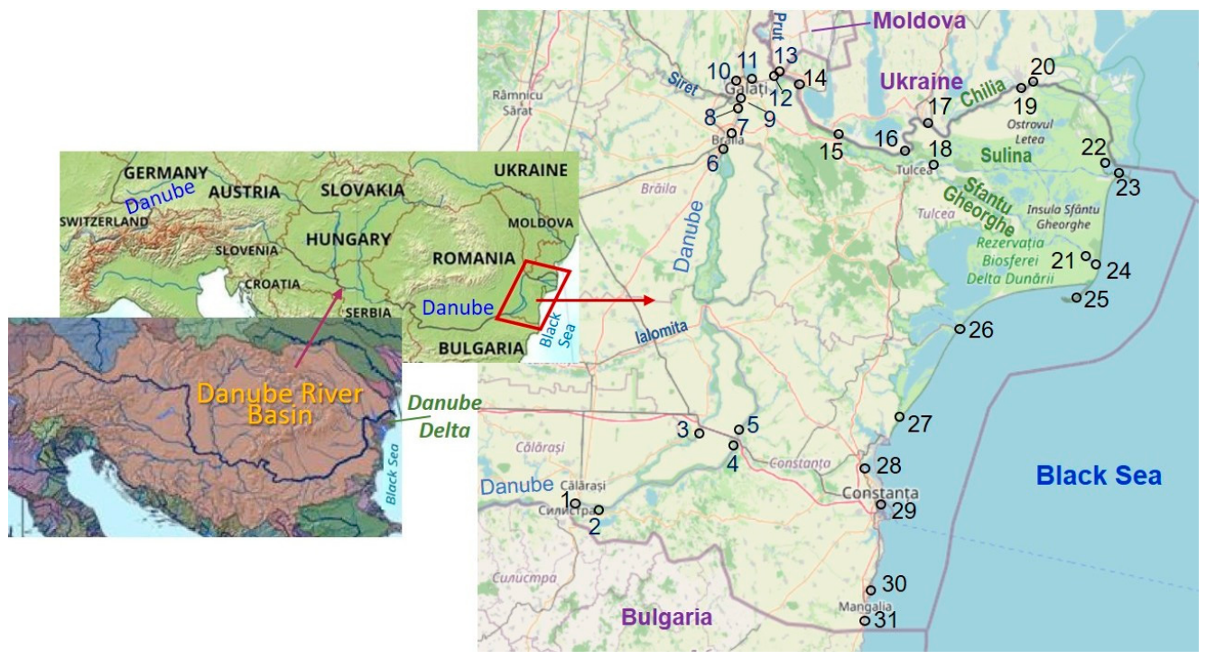
Figure 2.
Spatial distribution of the element mass fractions determined in the investigated fluvial and marine sediment samples (values on vertical axis are expressed in mg·kg-1).
Figure 2.
Spatial distribution of the element mass fractions determined in the investigated fluvial and marine sediment samples (values on vertical axis are expressed in mg·kg-1).
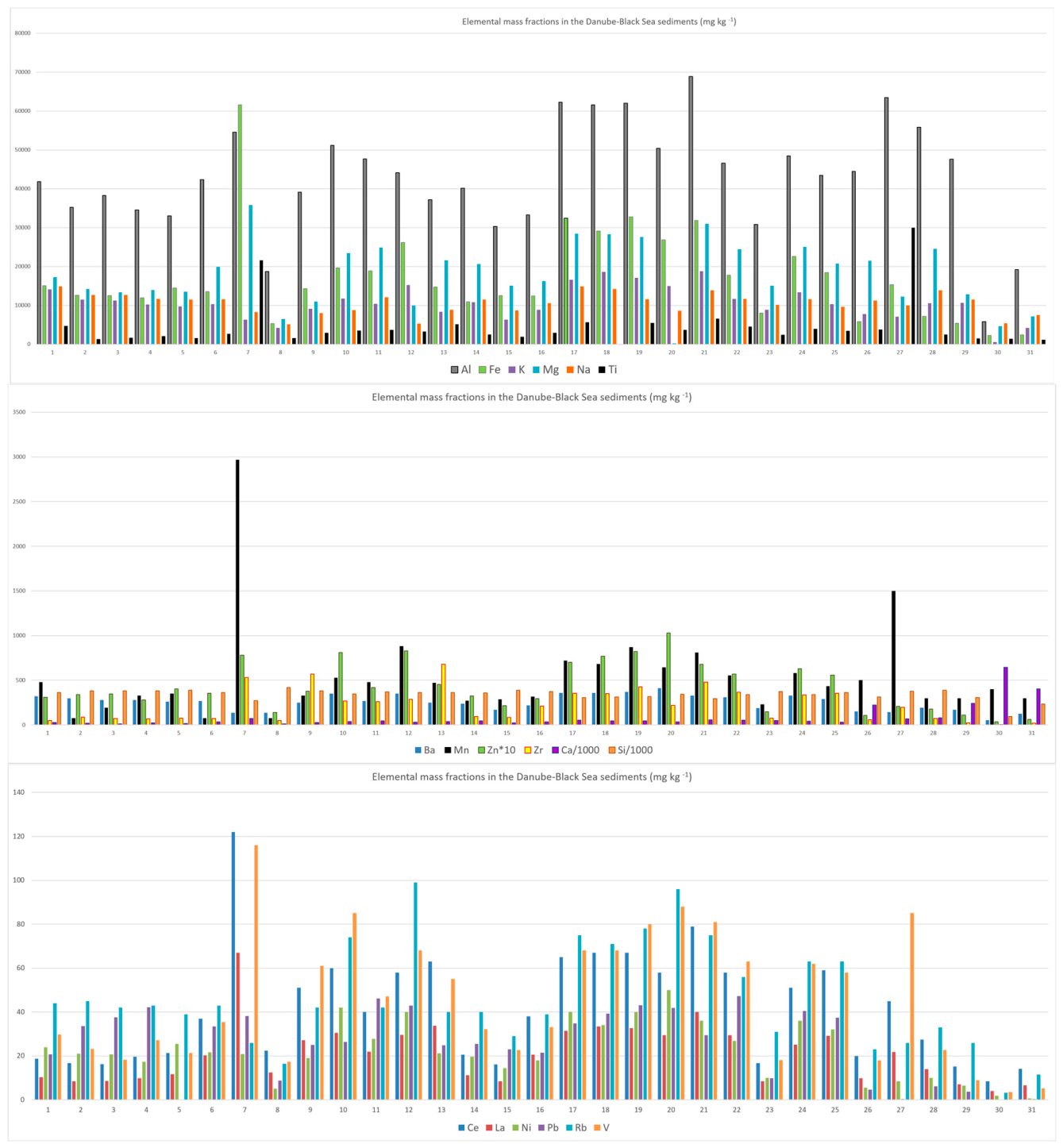
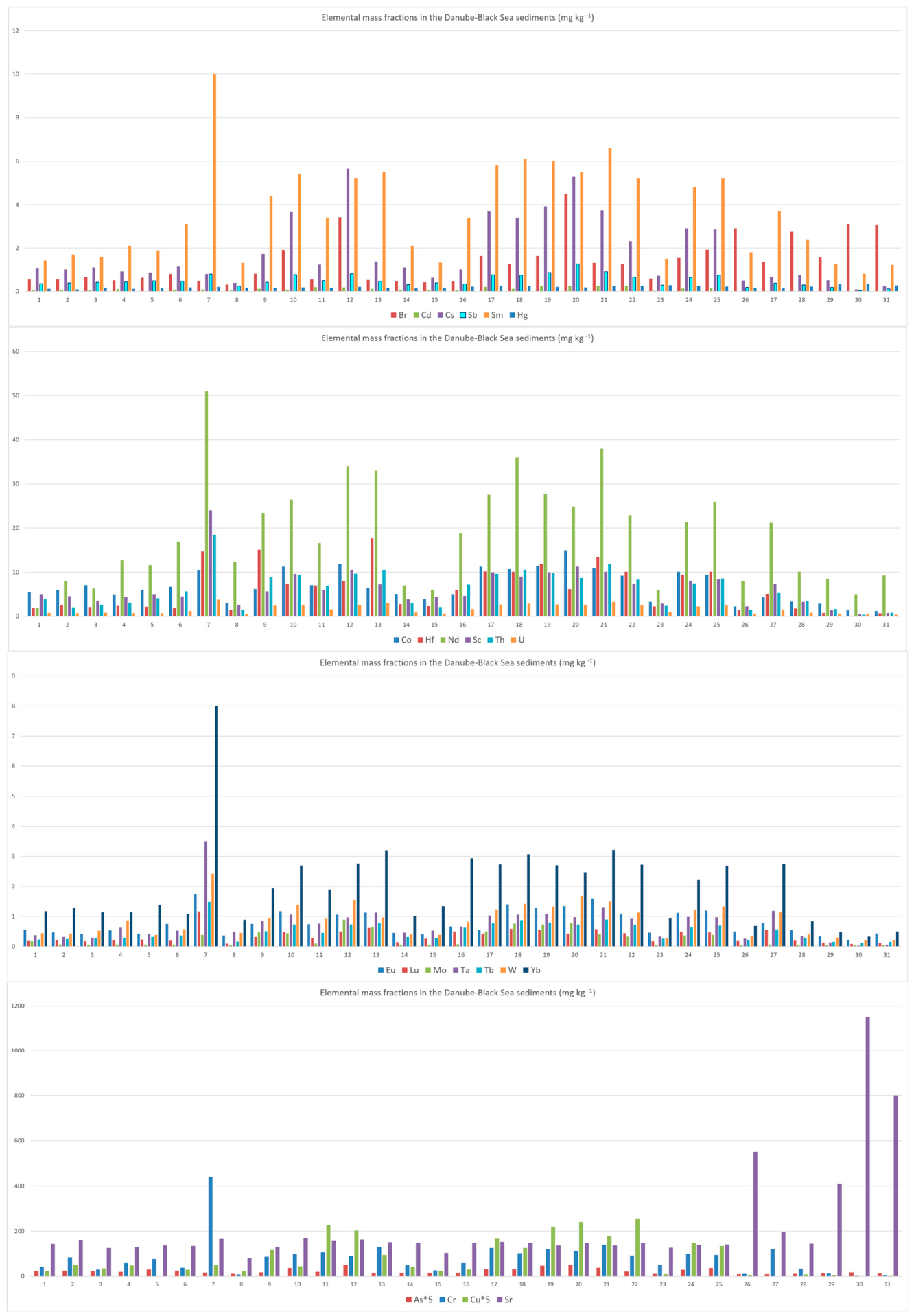
Figure 3.
Comparison of minimum, maximum, average and median values of the selected element mass fractions in the Danube sediment samples recorded in the present campaign (2019) and in 1996, reported by Pantelica et al., 1999 [20].
Figure 3.
Comparison of minimum, maximum, average and median values of the selected element mass fractions in the Danube sediment samples recorded in the present campaign (2019) and in 1996, reported by Pantelica et al., 1999 [20].
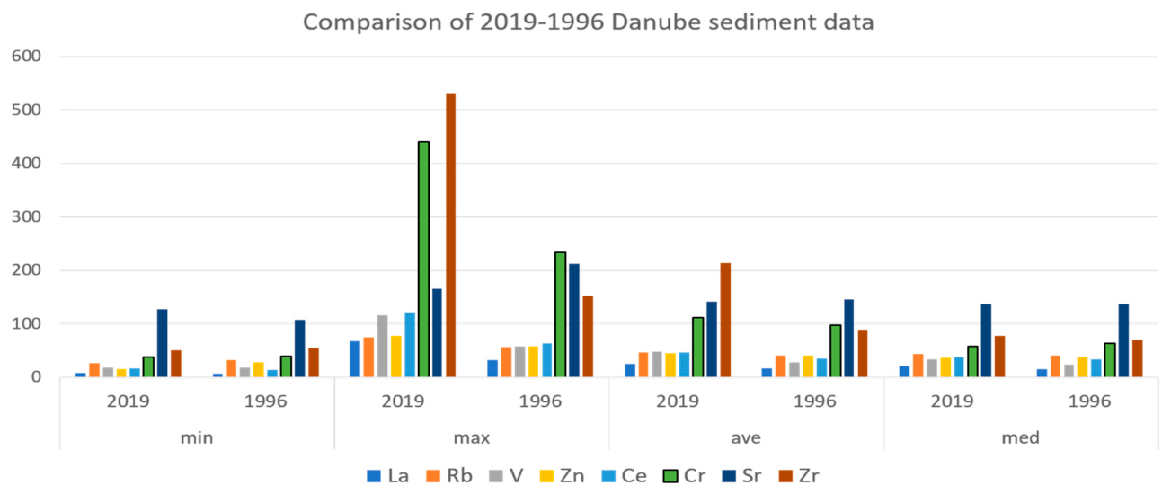
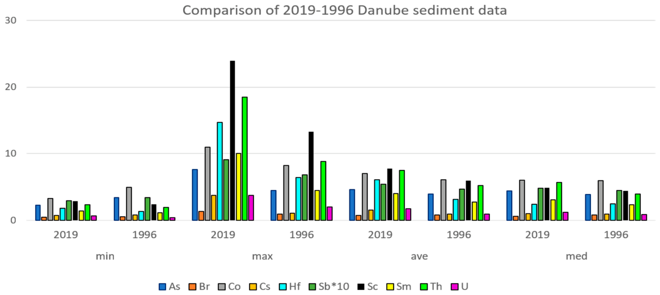
Figure 4.
Ratio of the selected element mass fractions determined in the Danube sediment samples in the present campaign (2019) and in 1996, reported by Pantelica et al., 1999 [20].
Figure 4.
Ratio of the selected element mass fractions determined in the Danube sediment samples in the present campaign (2019) and in 1996, reported by Pantelica et al., 1999 [20].
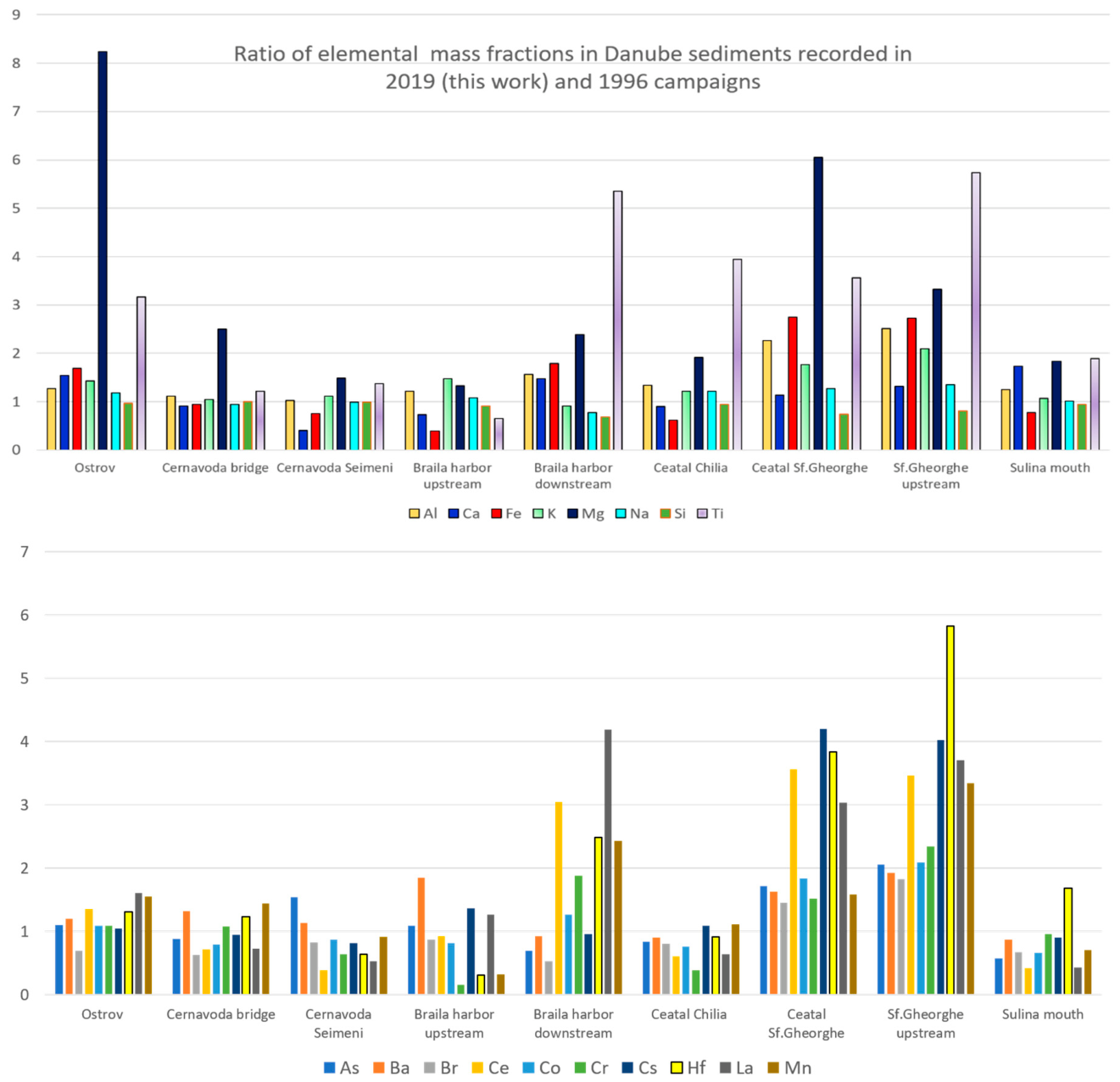
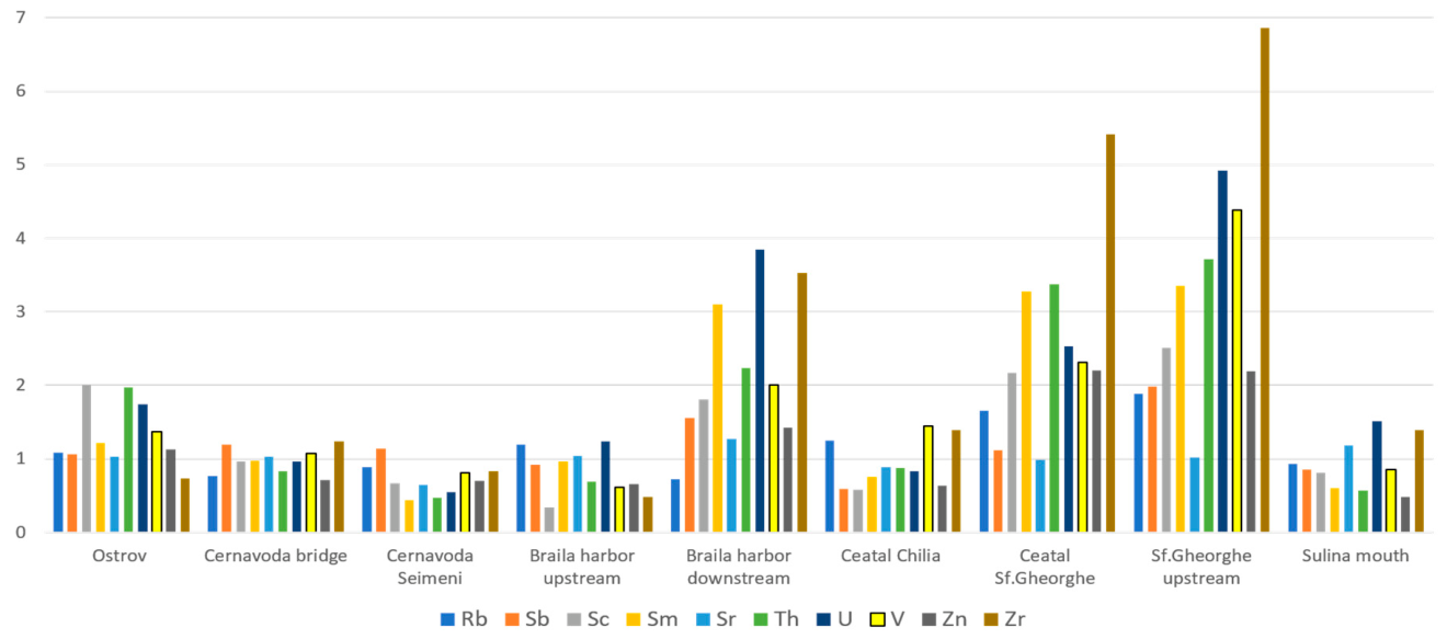
Figure 5.
Violin diagram of the Lower Danube major elements mass fraction normalized to UCC [54] (a); tree diagram illustrating the existence of two main clusters, SiO2 representing one of them (b); the log(Na2O\K2O) vs. log (SiO2\Al2O3) permitting a geochemical classification of the investigated Lower Danube unconsolidated sediments [69] (c); the Na2O/Al2O3 vs. K2O/Al2O3 biplot (d) [70].
Figure 5.
Violin diagram of the Lower Danube major elements mass fraction normalized to UCC [54] (a); tree diagram illustrating the existence of two main clusters, SiO2 representing one of them (b); the log(Na2O\K2O) vs. log (SiO2\Al2O3) permitting a geochemical classification of the investigated Lower Danube unconsolidated sediments [69] (c); the Na2O/Al2O3 vs. K2O/Al2O3 biplot (d) [70].
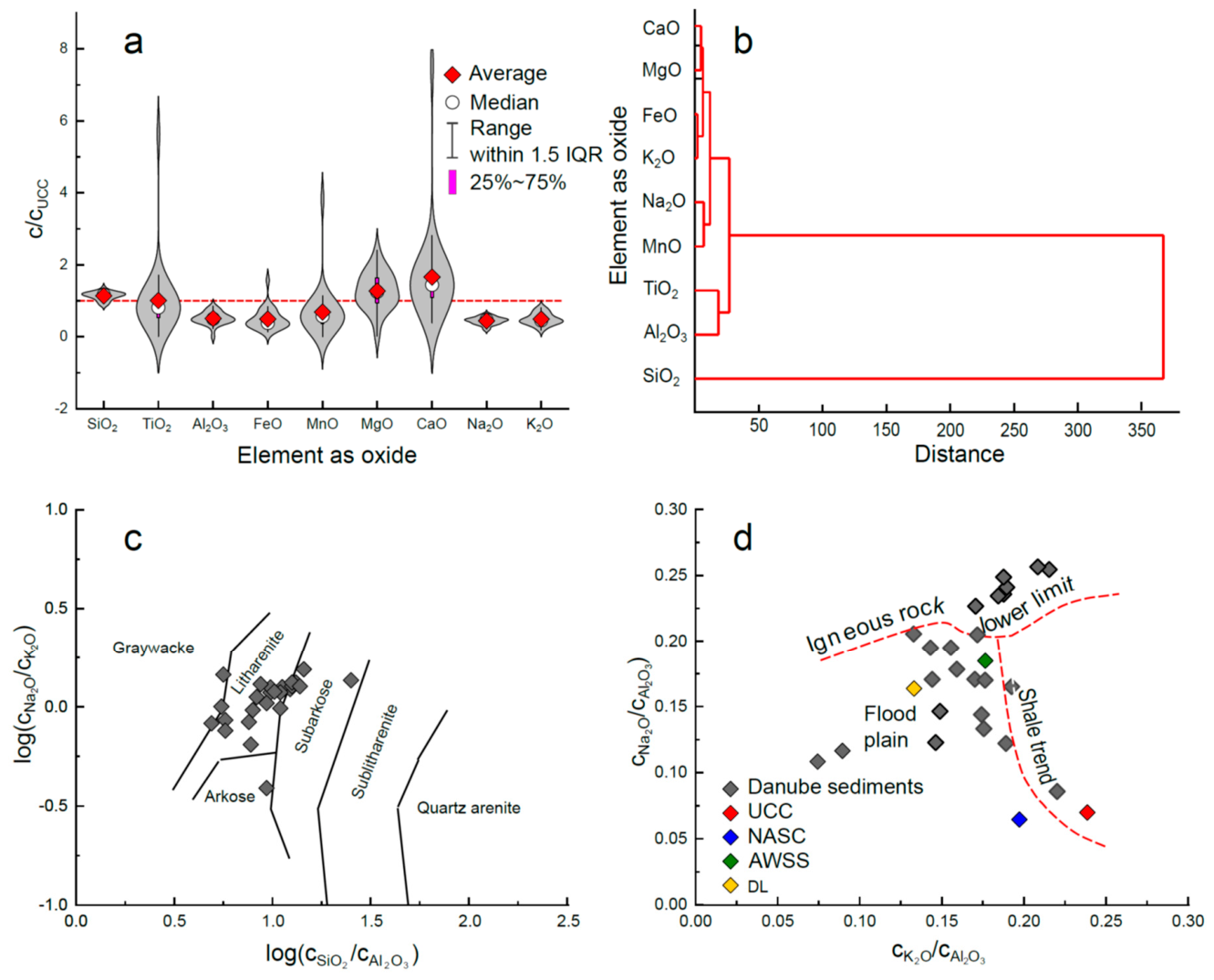
Figure 6.
Violin diagram illustrating the distribution of the major elements mass fraction normalized to UCC [54] in Black Sea marine sediments.
Figure 6.
Violin diagram illustrating the distribution of the major elements mass fraction normalized to UCC [54] in Black Sea marine sediments.
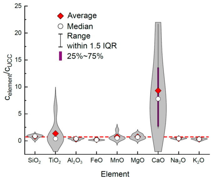
Figure 7.
Violin diagram illustrating the distribution of the investigated incompatible and HFSE (a) and PCE (b) elements in Danube River sediments. All mass fractions were normalized to UCC [54].
Figure 7.
Violin diagram illustrating the distribution of the investigated incompatible and HFSE (a) and PCE (b) elements in Danube River sediments. All mass fractions were normalized to UCC [54].
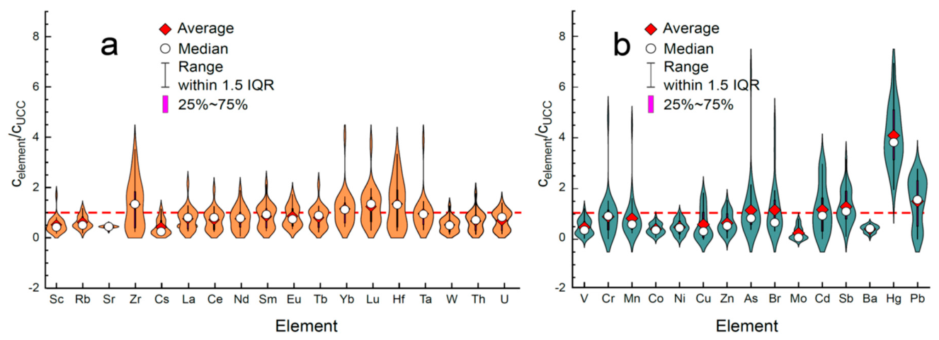
Figure 8.
Ternary discriminating diagram Sc-La-Th (a) [74], and V-Ni-10*Th (b) [75], biplots La/Th vs. Hf (c) [70], Th/Sc vs. Zr/Sc (d) [76], La vs. Th (e) [77], Th vs. U (f) [78], UCC normalized Lanthanides (h) [79] and Th vs. U (i) [78].
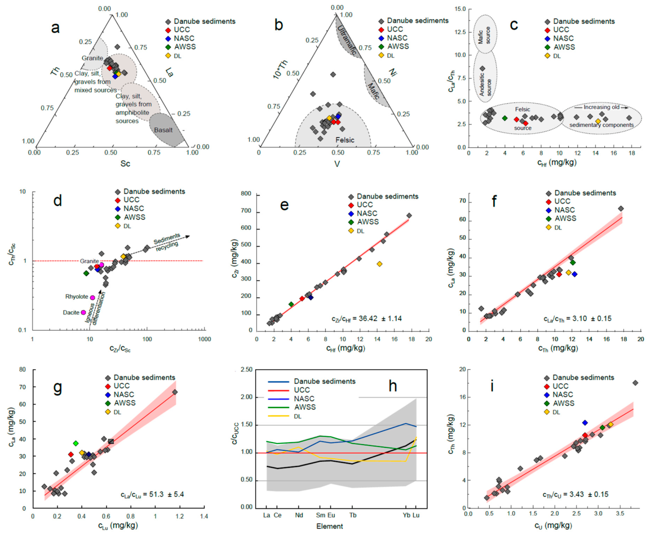
Figure 9.
Violin diagram illustrating the distribution of the investigated incompatible and HFSE (a) and PCE (b) elements in Black Sea marine sediments. All mass fractions were normalized to UCC [54].
Figure 9.
Violin diagram illustrating the distribution of the investigated incompatible and HFSE (a) and PCE (b) elements in Black Sea marine sediments. All mass fractions were normalized to UCC [54].
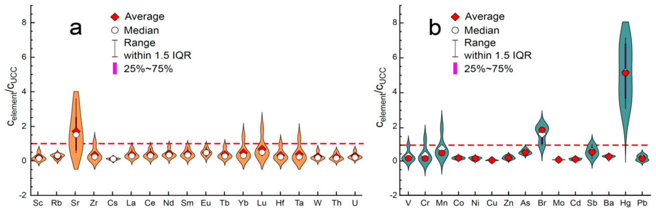
Figure 10.
The distribution of PLI along the minor valley of the Lower Danube River as well as Romanian Black Sea shore.
Figure 10.
The distribution of PLI along the minor valley of the Lower Danube River as well as Romanian Black Sea shore.
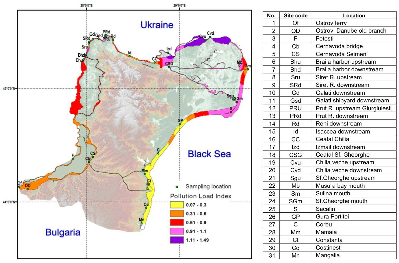
Figure 11.
The distribution of PLI along the minor valley of the Lower Danube River as well as Romanian Black Sea shore.
Figure 11.
The distribution of PLI along the minor valley of the Lower Danube River as well as Romanian Black Sea shore.
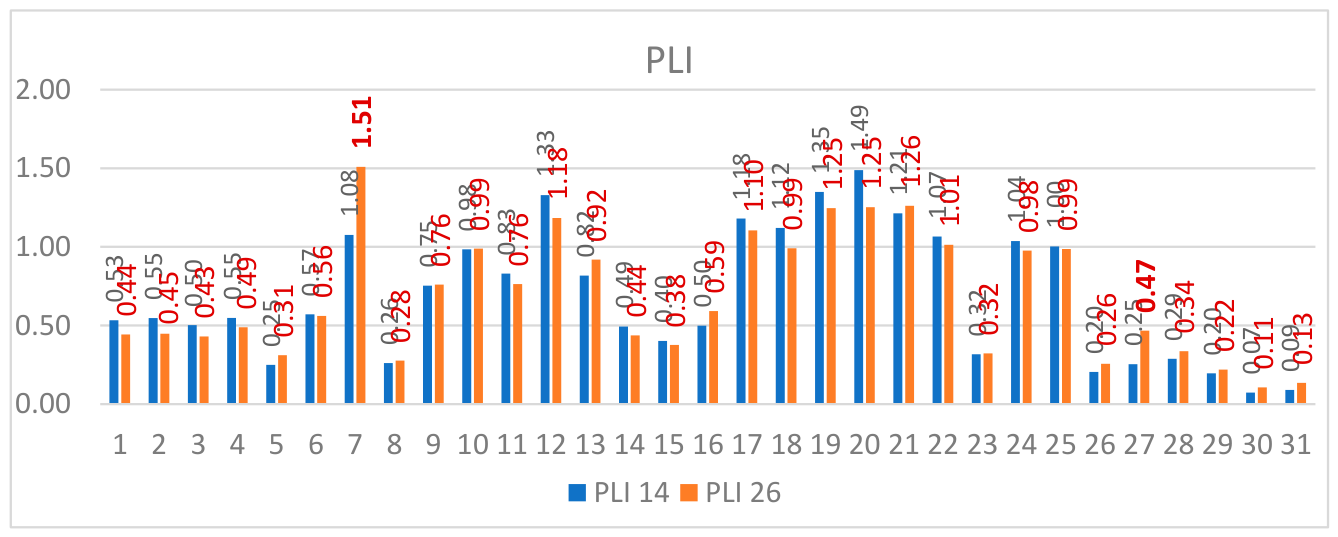
Figure 12.
The distribution of RI along the minor valley of the Lower Danube River and Romanian Black Sea shore.
Figure 12.
The distribution of RI along the minor valley of the Lower Danube River and Romanian Black Sea shore.
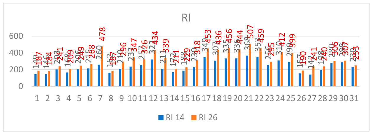
Figure 13.
The percentage contribution of Er to the total RI value for the 31 targeted sites; the REEs group is formed by the contribution of La, Ce, Nd, Sm, Eu, Tb, Yb, Lu.
Figure 13.
The percentage contribution of Er to the total RI value for the 31 targeted sites; the REEs group is formed by the contribution of La, Ce, Nd, Sm, Eu, Tb, Yb, Lu.
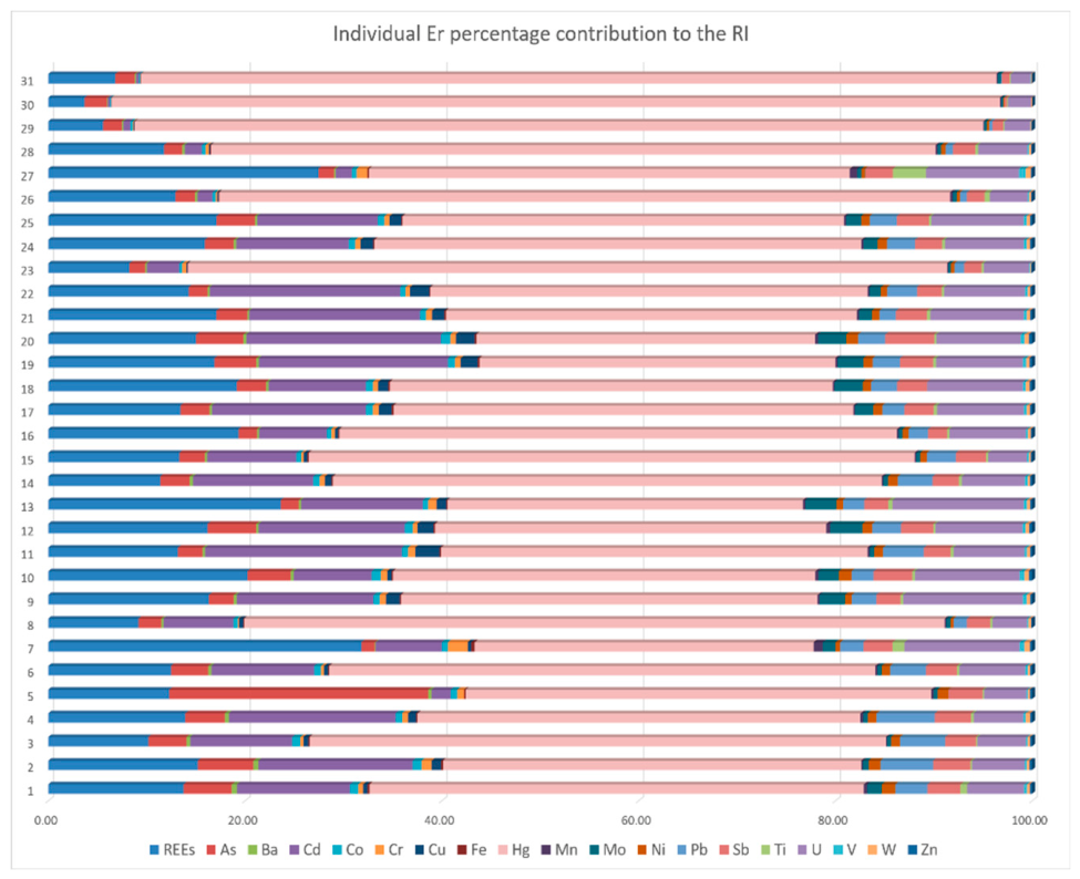
Figure 14.
The distribution of natural radionuclides activity concentration in sediments along the Lower Danube River and Romanian Black Sea shore.
Figure 14.
The distribution of natural radionuclides activity concentration in sediments along the Lower Danube River and Romanian Black Sea shore.
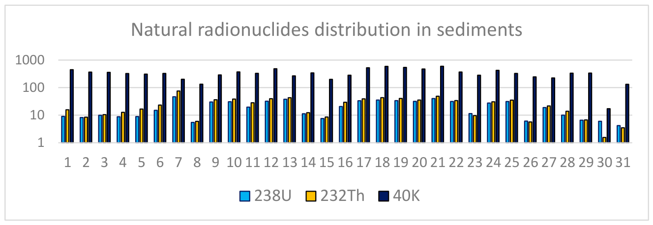
Table 1.
Description of the sampling sites.
| No. | Location | Longitude | Latitude |
|---|---|---|---|
| 1 | Ostrov ferry | 27.2770423065 | 44.1342510844 |
| 2 | Ostrov, Danube old branch | 27.3682014498 | 44.1132680431 |
| 3 | Fetesti | 27.8526166667 | 44.3776666667 |
| 4 | Cernavoda bridge | 28.0283325197 | 44.3514887492 |
| 5 | Cernavoda Seimeni | 28.0689945964 | 44.3968500445 |
| 6 | Braila harbor upstream | 27.9553333333 | 45.2288166667 |
| 7 | Braila harbor downstream | 27.9703166667 | 45.2549666667 |
| 8 | Siret R. upstream | 28.0242340642 | 45.3963383886 |
| 9 | Siret R. downstream | 28.0286048992 | 45.4106793422 |
| 10 | Galati downstream | 28.0683833333 | 45.4310000000 |
| 11 | Galati shipyard downstream | 28.1300166667 | 45.4383666667 |
| 12 | Prut R. upstream Giurgiulesti | 28.2025000000 | 45.4668666667 |
| 13 | Prut R. downstream | 28.2146666667 | 45.4671666667 |
| 14 | Reni downstream | 28.2861333333 | 45.4287000000 |
| 15 | Isaccea downstream | 28.4642833333 | 45.2838500000 |
| 16 | Ceatal Chilia | 28.7340333333 | 45.2284166667 |
| 17 | Izmail downstream | 28.8778166667 | 45.3137500000 |
| 18 | Ceatal Sf. Gheorghe | 28.8887500000 | 45.1876166667 |
| 19 | Chilia veche upstream | 29.2820000000 | 45.4265333333 |
| 20 | Chilia veche downstream | 29.3277532417 | 45.4506251037 |
| 21 | Sf.Gheorghe upstream | 29.5763316759 | 44.9023348772 |
| 22 | Musura bay mouth | 29.6447995422 | 45.1999407758 |
| 23 | Sulina mouth | 29.7352946497 | 45.1683710674 |
| 24 | Sf.Gheorghe mouth | 29.6175659223 | 44.8807156800 |
| 25 | Sacalin | 29.5540309449 | 44.7906880005 |
| 26 | Gura Portitei | 29.0090166667 | 44.6868833333 |
| 27 | Corbu | 28.7723666667 | 44.4274333333 |
| 28 | Mamaia | 28.6263833333 | 44.2459833333 |
| 29 | Constanta | 28.6735500000 | 44.1549333333 |
| 30 | Costinesti | 28.6421000000 | 43.9479166667 |
| 31 | Mangalia | 28.5922000000 | 43.8122666667 |
Table 2.
Quality assurance of INAA at the Regata facility, in mg·kg-1.
| Element | SRM | Determined | Uncertainty (%) | Certified | Uncertainty (%) | MDC |
|---|---|---|---|---|---|---|
| Na | 2709 | 9684 | 4.1 | 11600 | 2.6 | 20 |
| Mg | 1515 | 2699 | 4.4 | 2710 | 3 | 100 |
| Al | 2710 | 65319 | 5.3 | 64400 | 1.2 | 40 |
| Cl | 1547 | 347 | 8.2 | 360 | 5.3 | 44 |
| Si | 2709 | 303000 | 1.3 | 303000 | 9.8 | 88000 |
| K | 1515 | 15674 | 8 | 16100 | 1.2 | 980 |
| Ca | 1515 | 14518 | 14.5 | 15260 | 1 | 70 |
| Sc | 2709 | 11.9 | 5.5 | 12 | 3 | 0.005 |
| Ti | 2709a | 3116 | 6.8 | 3360 | 2.1 | 50 |
| V | 1632с | 23.9 | 4.6 | 23.72 | 2.2 | 0.11 |
| Cr | 667 | 189 | 6.3 | 178 | 9 | 1.3 |
| Mn | 1633b | 132.5 | 8.3 | 131.8 | 1.3 | 0.38 |
| Fe | 667 | 46198 | 5.4 | 44800 | 2.2 | 21 |
| Co | 667 | 23.7 | 5.5 | 23 | 5.6 | 0.01 |
| Ni | 667 | 134.9 | 6.8 | 128 | 7 | 0.48 |
| Zn | 667 | 177.6 | 4.4 | 175 | 7.4 | 0.4 |
| As | 2711a | 102 | 6 | 107 | 5 | 0.14 |
| Br | 667 | 82.8 | 4.4 | 99.7 | 2.5 | 0.1 |
| Rb | 2711a | 126 | 16.6 | 120 | 3 | 0.09 |
| Sr | 2709 | 244 | 9.2 | 231 | 0.9 | 1.4 |
| Sb | 667 | 1.031 | 5.1 | 0.96 | 5.2 | 0.002 |
| Zr | 2709a | 195 | 24.3 | 195 | 23.6 | 4.0 |
| Mo | 2710 | 19 | 3 | 18.6 | 2.7 | 0.08 |
| Cs | 667 | 8.6 | 3 | 7.8 | 9 | 0.005 |
| Ba | FFA-1 | 792 | 11.1 | 835 | 6.7 | 1.2 |
| La | FFA-1 | 61.3 | 3.8 | 60.7 | 6.6 | 0.03 |
| Ce | FFA-1 | 122 | 5.6 | 120 | 5.8 | 0.4 |
| Sm | FFA-1 | 8.2 | 17 | 10.9 | 5.5 | 0.001 |
| Ta | FFA-1 | 8.3 | 6.1 | 6.2 | 7.4 | 0.002 |
| Nd | FFA-1 | 56.8 | 6.5 | 55.7 | 6.1 | 0.01 |
| Eu | 2709a | 0.98 | 8.3 | 0.83 | 2.4 | 0.01 |
| Tb | FFA-1 | 1.38 | 10.1 | 1.39 | 10.5 | 0.002 |
| Yb | FFA-1 | 4.24 | 4.4 | 4.16 | 5.1 | 0.002 |
| Lu | FFA-1 | 0.658 | 6.65 | 0.66 | 6.3 | 0.002 |
| Hf | FFA-1 | 7.3 | 6.1 | 6.2 | 7.4 | 0.01 |
| W | FFA-1 | 10.5 | 11.1 | 10.2 | 10.5 | 0.001 |
| Th | 667 | 10.2 | 4.7 | 10 | 5 | 0.005 |
| U | 2711a | 3.007 | 8.5 | 3.01 | 4 | 0.03 |
| Indices | Formula | Definition | Risk categories/ Site pollution degree |
|---|---|---|---|
| Contamination factor (CF) | (1) | Contamination factor CF(i) of an individual element (i) is the ratio between the measured concentration of each element concentration, , in the sediment sample and its background (baseline) concentration, (i=1÷n; n=number of chemical elements of interest) | Low, CF<1 Moderate, 1 ≤ CF < 3 Considerable, 3 ≤ CF < 6 Very high, CF ≥ 6 |
| Pollution Load Index (PLI) | (2) | Pollution Load Index for a site #Sk is the nth root of the product of the individual contamination factors calculated for target PCEs (n=number of PCEs/ contamination factors). | Not polluted, PLI<1 Baseline level, PLI=1 Polluted, PLI>1 |
| Regional Pollution Load Index (RPLI) | (3) | Regional Pollution Load Index for a study area (region/sector/zone) #z is the mth root of the product of the PLIs of individual site average (k=1÷m; m= number of sampling sites comprised in the respective area). | Not polluted, RPLI<1 Baseline level, RPLI=1 Polluted, RPLI>1 |
| Ecological risk factor () | (4) | Ecological risk factor () for an element i measures the potential ecological risk of a single given toxic (contaminant) element i in sediment and it is defined as the product of the contamination factor () and the toxic-response factor () for that specific element. | Low, Er < 40 Moderate, 40 ≤ Er < 80 Considerable, 80 ≤ Er < 160 High, 160 ≤ Er < 320 Very high, Er ≥ 320 |
| Potential Ecological Risk Index (RI) | (5) | The (total) Potential Ecological Risk Index (RI) is the sum of the individual ecological risk factors () of the n considered PCEs. | Low, RI < 150 Moderate, 150 ≤ RI < 300 Strong, 300 ≤ RI < 600 Very strong, 600 ≤ RI < 1200 Highly strong, RI ≥ 1200 |
Table 4.
Activity concentrations A(U), A(Th) and A(K) (Bq⋅kg−1) of natural radionuclides 238U, 232Th and 40K and associated radiological hazard parameters − Raeq (Bq⋅kg−1), ADR (nGy h−1), Hex, IG, AED (mSv y−1), ELCR.
Table 4.
Activity concentrations A(U), A(Th) and A(K) (Bq⋅kg−1) of natural radionuclides 238U, 232Th and 40K and associated radiological hazard parameters − Raeq (Bq⋅kg−1), ADR (nGy h−1), Hex, IG, AED (mSv y−1), ELCR.
| Site | A(U) (Bq kg−1) |
A(Th) (Bq kg−1) |
A(K) (Bq kg−1) |
Raeq (Bq kg−1) |
ADR (nGy h−1) |
IG | Hex | AED (mSv y−1) |
ECLR |
|---|---|---|---|---|---|---|---|---|---|
| Ostrov ferry | 9.0 | 15.6 | 447.2 | 65.8 | 32.25 | 0.51 | 0.18 | 0.040 | 0.000138 |
| Ostrov, Danube old branch | 8.2 | 8.4 | 364.8 | 48.3 | 24.07 | 0.38 | 0.13 | 0.030 | 0.000103 |
| Fetesti | 9.9 | 10.4 | 357.1 | 52.3 | 25.75 | 0.41 | 0.14 | 0.032 | 0.000111 |
| Cernavoda bridge | 8.8 | 12.6 | 324.9 | 51.8 | 25.22 | 0.40 | 0.14 | 0.031 | 0.000108 |
| Cernavoda Seimeni | 8.9 | 16.6 | 307.8 | 56.4 | 27.00 | 0.43 | 0.15 | 0.033 | 0.000116 |
| Braila harbor upstream | 15.0 | 23.2 | 326.9 | 73.2 | 34.52 | 0.55 | 0.20 | 0.042 | 0.000148 |
| Braila harbor downstream | 46.6 | 75.3 | 201.5 | 169.7 | 75.39 | 1.20 | 0.46 | 0.092 | 0.000324 |
| Siret R. upstream | 5.4 | 5.9 | 132.9 | 24.2 | 11.64 | 0.18 | 0.07 | 0.014 | 0.000050 |
| Siret R. downstream | 30.0 | 36.2 | 289.2 | 104.1 | 47.81 | 0.76 | 0.28 | 0.059 | 0.0805 |
| Galati downstream | 30.8 | 38.2 | 371.9 | 114.1 | 52.83 | 0.84 | 0.31 | 0.065 | 0.0827 |
| Galati shipyard downstream | 19.5 | 28.1 | 329.1 | 85.0 | 39.70 | 0.63 | 0.23 | 0.049 | 0.000170 |
| Prut R. upstream Giurgiulesti | 32.0 | 39.5 | 482.6 | 125.6 | 58.75 | 0.93 | 0.34 | 0.072 | 0.0852 |
| Prut R. downstream | 37.7 | 42.7 | 266.2 | 119.3 | 54.32 | 0.86 | 0.32 | 0.067 | 0.0833 |
| Reni downstream | 11.2 | 12.2 | 342.4 | 55.1 | 26.87 | 0.43 | 0.15 | 0.033 | 0.000115 |
| Isaccea downstream | 7.5 | 8.5 | 200.1 | 35.2 | 16.99 | 0.27 | 0.09 | 0.021 | 0.000073 |
| Ceatal Chilia | 20.6 | 29.3 | 282.3 | 84.3 | 39.00 | 0.62 | 0.23 | 0.048 | 0.000167 |
| Izmail downstream | 33.4 | 39.1 | 526.0 | 129.7 | 60.94 | 0.96 | 0.35 | 0.075 | 0.0862 |
| Ceatal Sf.Gheorghe | 35.3 | 43.1 | 589.2 | 142.4 | 66.95 | 1.06 | 0.38 | 0.082 | 0.0887 |
| Chilia veche upstream | 33.5 | 40.3 | 540.6 | 132.7 | 62.35 | 0.99 | 0.36 | 0.076 | 0.0868 |
| Chilia veche downstream | 31.8 | 35.4 | 473.6 | 118.8 | 55.80 | 0.88 | 0.32 | 0.068 | 0.0840 |
| Sf.Gheorghe upstream | 40.2 | 48.4 | 595.9 | 155.3 | 72.65 | 1.15 | 0.42 | 0.089 | 0.000312 |
| Musura bay mouth | 31.4 | 33.8 | 368.5 | 108.1 | 50.27 | 0.79 | 0.29 | 0.062 | 0.0816 |
| Sulina mouth | 11.4 | 9.6 | 282.4 | 46.9 | 22.85 | 0.36 | 0.13 | 0.028 | 0.000098 |
| Sf.Gheorghe mouth | 27.6 | 30.5 | 424.4 | 103.9 | 48.86 | 0.77 | 0.28 | 0.060 | 0.0810 |
| Sacalin | 31.1 | 35.0 | 327.4 | 106.4 | 49.17 | 0.78 | 0.29 | 0.060 | 0.0811 |
| Gura Portitei | 6.1 | 5.7 | 245.0 | 33.0 | 16.44 | 0.26 | 0.09 | 0.020 | 0.000071 |
| Corbu | 18.9 | 21.6 | 225.2 | 67.1 | 31.15 | 0.49 | 0.18 | 0.038 | 0.000134 |
| Mamaia | 10.0 | 13.8 | 334.7 | 55.6 | 26.94 | 0.43 | 0.15 | 0.033 | 0.000116 |
| Constanta | 6.6 | 6.7 | 336.9 | 42.1 | 21.14 | 0.34 | 0.11 | 0.026 | 0.000091 |
| Costinesti | 6.0 | 1.5 | 17.1 | 9.5 | 4.41 | 0.07 | 0.03 | 0.005 | 0.000019 |
| Mangalia | 4.2 | 3.5 | 132.3 | 19.3 | 9.54 | 0.15 | 0.05 | 0.012 | 0.000041 |
| min | 4.2 | 1.5 | 17.1 | 9.5 | 4.4 | 0.07 | 0.03 | 0.01 | 0.008 |
| max | 46.6 | 75.3 | 596 | 169.7 | 75.4 | 1.20 | 0.46 | 0.09 | 0.00032 |
| ave | 20.3 | 24.9 | 337 | 81.8 | 38.4 | 0.61 | 0.22 | 0.05 | 0.00016 |
| SD | 12.8 | 17.0 | 132.8 | 42.8 | 19.4 | 0.31 | 0.12 | 0.02 | 0.00008 |
| med | 19 | 23 | 329 | 73 | 35 | 0.55 | 0.20 | 0.04 | 0.00015 |
| CV (%) | 63.1 | 68.5 | 39.4 | 52.4 | 50.5 | 50.45 | 52.36 | 50.48 | 50.48 |
| Recommended [83,84] | 35 | 30 | 400 | 370 | 57 | 1 | 1 | 0.070 | 2.9×10⁻⁴ |
Disclaimer/Publisher’s Note: The statements, opinions and data contained in all publications are solely those of the individual author(s) and contributor(s) and not of MDPI and/or the editor(s). MDPI and/or the editor(s) disclaim responsibility for any injury to people or property resulting from any ideas, methods, instructions or products referred to in the content. |
© 2026 by the authors. Licensee MDPI, Basel, Switzerland. This article is an open access article distributed under the terms and conditions of the Creative Commons Attribution (CC BY) license (http://creativecommons.org/licenses/by/4.0/).
Copyright: This open access article is published under a Creative Commons CC BY 4.0 license, which permit the free download, distribution, and reuse, provided that the author and preprint are cited in any reuse.


