

Submitted:
25 June 2026
Posted:
26 June 2026
You are already at the latest version
Abstract
Acoustic Emission (AE) measurements have many uses to evaluate the integrity of mate-rials. AE is often used to detecting leakage in pipelines. It has also been used to monitor changes in strength properties of fiber reinforced concrete. In the oil and gas industry, AE is predominantly used to study fracture initiation and propagation. In particular, charac-terization of samples is key for evaluating subsurface formations for successful under-ground storage. Research has been done to understand the behavior of AE in uniaxial compression and single stage triaxial compression tests. However, the validity of this method has not been documented in a multistage triaxial test. This characterization is required to understand the stability of the host rock under the related stress changes and potential mineralogic changes which may occur. Typically, there is a shortage of geolog-ic samples. A single multistage triaxial test eliminates the need for twin samples and provides an economic and time saving protocol compared to conventional methods. A single multi-stage triaxial (MST) test allows a constitutive model to be developed for a host rock. This work establishes a protocol for performing these tests with minimal correc-tions to the measurements. Acoustic Emissions were measured on five different samples undergoing Multi-stage Triaxial Tests. Two different behaviors were observed. For the “coarse grained” samples, designated Group 1 (Miocene sandstone, Wilcox and Cambri-an sandstone), the number of AE events did not show a strong dependence on confining stress. They did show an exponential increase of AE events with increasing deviatoric stress during each stage. In contrast, the Group 2 samples (Niobrara Marl and Niobrara Chalk) exhibited a significantly different stress dependent AE behavior. The amplitude of the AE events is significantly smaller than the quartz dominated samples indicating a more ductile and diffuse failure mechanism. The correction between maximum compres-sive strength and the point of positive dilatancy is still 1.2 for these samples, even though a different pattern of AE events is observed.
Keywords:
acoustic emissions
; triaxial test
1. Introduction
Understanding the geomechanical behavior of rocks under in-situ stress conditions is critical for petroleum geomechanics, underground excavation, geothermal systems, mining, carbon sequestration, and subsurface energy storage. Mechanical properties such as Young’s modulus, Poisson’s ratio, unconfined compressive strength, pore pressure response, and elastic-wave velocities are commonly determined using triaxial compression tests, where axial stress is increased under constant confining pressure until failure (Fjaer et al., 2008). Conventional triaxial testing, however, requires multiple specimens to define a complete failure envelope, which is problematic for limited or heterogeneous cores. Multistage triaxial testing (MST) addresses this limitation by evaluating several stress states using a single specimen (Alsalman et al., 2015). In MST, the specimen is repeatedly loaded, unloaded, and reloaded under increasing confinement, though accumulated damage may influence later stages. Unloading criteria commonly include the onset of dilation, inflection points, or maximum-curvature points associated with crack initiation and nonlinear deformation (Kovari & Tisa, 1975; Youn & Tonon, 2010; Vakilinezhad, 2022). Because significant internal damage may occur before visible failure, acoustic emission (AE) monitoring provides an effective means of tracking progressive damage during MST.
AE refers to transient elastic waves generated by rapid strain-energy release during localized deformation. In rocks, AE is associated with crack initiation, crack growth, grain crushing, pore collapse, frictional sliding, and crack coalescence (Lockner, 1993; Michlmayr et al., 2012). AE signals generally range from 10–1000 kHz and provide a non-invasive method for monitoring internal damage evolution. Early studies showed that AE activity accelerates near failure and follows statistical relations similar to earthquakes (Mogi, 1962; Scholz, 1968). Lockner (1993) later established AE as a major experimental tool for investigating crack nucleation and fracture evolution in rocks.AE activity evolves systematically during deformation. Initial loading is dominated by crack closure and low AE activity, followed by stable crack growth and increasing AE counts. Near failure, AE accelerates rapidly as cracks localize and coalesce (Lockner, 1993; Read et al., 1995; Zang et al., 2000). Sun et al. (2023) identified compaction, rising activity, peak activity, and descending AE stages in granite and sandstone, with AE quiet zones preceding failure. Ohnaka and Mogi (1982), Li and Nordlund (1993), and Read et al. (1995) further showed that AE frequency characteristics evolve significantly with stress level and crack propagation, while Zang et al. (2000) distinguished brittle fracture from frictional sliding using AE duration and energy characteristics. AE monitoring can distinguish deformation mechanisms through variations in event rate, energy, amplitude, duration, and frequency content. Liakopoulou-Morris et al. (1994) related AE waveform evolution to fracture localization in sandstone, while Stanchits et al. (2006) linked AE activity to crack-density evolution and ultrasonic velocity reduction. Wang et al. (2021) showed that decreasing Gutenberg–Richter b-values correspond to the transition from distributed microcracking to unstable macrofracture formation, with low-frequency AE signals associated with shear fractures and high-frequency signals linked to tensile cracking. AE generation mechanisms in rocks are diverse and include grain-contact rearrangement, frictional sliding, rupture of cementation bonds, grain crushing, and crack formation (Michlmayr et al., 2012). In porous rocks, pore collapse and cataclastic deformation also contribute significantly (Baud et al., 2004; Fortin et al., 2006). Guo and Zhao (2022) showed that granite generates more AE activity than sandstone or marble because of its abundant pre-existing microcracks, although tensile cracking dominated across all lithologies.
In granular geomaterials, stress is transmitted through heterogeneous force-chain networks whose collapse and reformation generate significant AE activity (Behringer et al., 1999; Hidalgo et al., 2002; Tordesillas, 2007; Tordesillas et al., 2009; Welker & McNamara, 2011). Crack formation remains the dominant AE mechanism during brittle failure, while increasing confining pressure suppresses unstable tensile cracking and promotes distributed shear deformation (Amitrano, 2003; Brantut et al., 2011). Zhao et al. (2023) showed that crack initiation and damage thresholds increase with confining pressure, whereas AE activity remains low during stable crack growth before accelerating sharply near failure. AE has also been widely applied to compaction and grain crushing in porous rocks. Baud et al. (2004) and Fortin et al. (2006) demonstrated that pore collapse and permeability reduction are associated with distinct AE evolution. Zhang et al. (2023) further showed that increasing confining pressure strengthens sandstone, whereas pore-water pressure weakens the rock and suppresses AE activity, as water softening reduces abrupt elastic energy release during crack propagation. The statistical behavior of AE provides important insights into the evolution of progressive damage. Numerous studies have shown that AE amplitudes and energies follow Gutenberg–Richter-type power-law distributions (Mogi, 1962; Scholz, 1968; Lockner, 1993). Decreasing b-values are commonly associated with increasing crack localization and coalescence (Main et al., 1989; Amitrano, 2003; Lavrov & Shkuratnik, 2005). Zhang et al. (2015) demonstrated that AE evolution during uniaxial and triaxial loading exhibits fractal scaling behavior, with increasing localization preceding failure. Waiting-time distributions and AE energy statistics have also been linked to avalanche-like crack interaction and self-organized criticality (Bak et al., 1987; Johansen & Sornette, 2000; Anifrani et al., 1995). Liu and Meng (2024) further showed that AE signals exhibit multifractal characteristics that systematically evolve with the loading path and crack-network complexity. Confining pressure strongly influences AE behavior. At low confinement, brittle tensile cracking dominates and AE acceleration near failure is rapid. Higher confinement promotes more distributed crack growth, frictional sliding, grain crushing, and compaction processes (Amitrano, 2003; Baud et al., 2004; Brantut et al., 2011). Consequently, AE signatures evolve significantly with confinement and stress path, making AE monitoring particularly valuable for MST applications.
Despite extensive research on AE during uniaxial and conventional triaxial compression, relatively few studies have investigated AE during MST. This is important because MST subjects a single specimen to repeated loading cycles that may progressively accumulate irreversible damage. AE is uniquely suited to investigate this process because it directly detects internal microstructural damage not visible in stress–strain measurements alone. The present study integrates AE monitoring with MST to evaluate the implications of different unloading criteria. AE hits, cumulative counts, energy, and statistical parameters are used as indicators of progressive damage accumulation. The study compares unloading at the maximum-curvature point, the PPD criterion, and the maximum compressive-strength point to identify an unloading criterion that minimizes irreversible damage while still accurately defining the yield surface and failure envelope.
2. Materials and Methods
2.1. Experimental Setup
Figure 1 is a sketch of the experimental setup. The axial load is applied to a one-inch diameter by two-inch-long cylindrical sample. A constant axial strain rate loading parameter is used for these tests. The radial (confining stress) is applied using Multitherm IG-4©.
2.2. Strain Measurements
Axial strain is measured by two Linear Variable Differential Transducers (LVDTs) mounted on the end-caps (Figure 1). Average of both LVDTs determines the axial strain. A four-arm cantilever bridge is used to measure radial strain at two different points. A positive strain is defined as a decreasing sample dimension. The axial strain under loading is therefore positive and the radial strain is negative. Volumetric strain is a calculated parameter. A 30,000 lb. vented internal load cell measures the applied load. All strain measurements are calibrated. They are adjusted for endcap strain and confining pressure corrections using a Tungsten billet and then verified by measuring an Aluminum billet.
The point of positive dilatancy (PPD) shown in Figure 2 is used as the unloading point for each stage in the multistage triaxial measurements. PPD is defined as the point where the strain ratio between radial and axial strain reaches 0.5. When the radial to axial strain ratio reaches 0.5 the sample volume change is zero. (Bilal, 2016).
2.3. AE Equipment
The AE equipment used in this research is a portable 1283 USB node© manufactured by Physical Acoustics. It consists of an AE sensor, a SMA-SMB coaxial cable, USB node and USB connector (Figure 2.7). The USB node is connected to a laptop and runs of battery power. A single sensor with a resonant frequency of 150 kHz (model- R15 alpha) is used in this work. The sensor is mounted on the bottom end-cap (Figure 2.1). The sensor is connected to the USB node via a SMA-SMB coaxial cable. The USB node is connected to a laptop using conventional USB cable. This setup is isolated from the main computer that runs the MR compaction software.
The device is operated from the laptop using the vendor supplied software, AEWin©. Data is collected between a bandwidth of 100-300 kHz with an amplitude threshold of 25dB. The sample rate is set to be at 5 mega-samples per second and the pre-trigger is at 50 micro-seconds. Length of the wavelet collected is capped at 5000 points (Figure 2.8).
2.3. Attributes of an AE Waveform
There are many attributes in an acoustic emission event (Pollock, 1989). These are AE hits, amplitude threshold, rise time, total energy, duration of the event and total number of counts (Figure 3). Amplitude threshold is a user defined parameter, defined to maximize the number of true events detected minimizing triggering on noise. This was optimized at 25dB. When an AE waveform crosses this amplitude threshold, it is recorded and registered as an event. Rise time is the time difference between the first recorded peak, when the wave amplitude is higher than the amplitude threshold and the peak amplitude of the wave. The area under the curve that exceeds the threshold amplitude in a waveform is the total energy of the waveform. Duration of the event is the time difference between the first crest that crosses the threshold amplitude and the last crest that does the same. Total counts is the total number of crests that have higher amplitude than the amplitude threshold in an AE waveform.
2.4. Samples
Five different formations with varying characteristics were measured. A Miocene aged sandstone (WEEKS ISLAND) is a Tertiary Gulf of Mexico (GOM) sandstone. It is weakly cemented and very well sorted. (BURHAN) is a medium grained Cambrian sandstone. It is very well consolidated with intergranular pressure solution and quartz cement. The Wilcox sandstone (WILCOX) is a fine grained Paleogene (Tertiary) sandstone in deep-water GOM. It has a small amount of quartz cement and high amounts of lithic fragments and is poorly sorted. Deformation bands have been known to occur in the sub-surface.
The fine-grained samples consist of Niobrara Marl and Niabrara Chalk. Niobrara Marl (NIO) is a Cretaceous calcareous mudrock. This Marl facies has high Total Organic Content (TOC) and high 30% to 40% clay content. This marl is dominated by porosity associated with clay minerals. Presence of TOC and clays make this formation more ductile in nature. This sample was collected from an outcrop in Colorado. Niobrara Chalk (NICH) is a Cretaceous Chalk. It’s close to a 100% carbonate with a very small amount of clay and absence of any organic material. It has a higher inter-particle porosity than the Marl. This sample was also collected from an outcrop in Colorado.
2.5. Sample Preparation
Cores were drilled to a two inch length by one inch diameter. An end trim is cut for pre-test thin section analysis. The ends were surface ground and polished to achieve better acoustic contact with the endcaps. The pre-test samples were all imaged in the Micro-CT scanner (Zeiss Xradia 510 Versa©). The sample is placed between triaxial steel end caps and sealed using a viton sleeve. Another layer of viton© sleeves is placed over the endcap O-rings to prevent leakage of confining fluid into the sample. The sensors and gauges are placed on the sample (Figure 2.1). This setup is placed inside the pressure vessel.
2.6. Multi-Stage Triaxial Testing Protocol
After the measurement stack is assembled the pressure vessel is filled with confining fluid. The confining pressure is then raised to 500 psi (1st stage) and a deviatoric stress is raised to 100 psi. The sample is loaded at a constant axial strain rate up to the the point of positive dilatancy (PPD). Unloading starts at this point and ends at a low deviatoric stress (100 psi). The confining pressure is then raised and the 2nd stage (1000 psi) is performed. A total of seven different confining pressure stages are performed – 500 psi, 1000 psi, 1500 psi, 2000 psi, 2500 psi, 3000 psi and 4000 psi. The last loading-unloading loop (3000 – 4000 psi) is repeated. The sample is taken to failure at the 4000 psi confining pressure of 4000 psi and then unloaded to a low deviatoric stress and removed from the pressure vessel. The posttest sample is imaged in the Micro-CT scanner and thin sections are prepared for visual analysis.
2.7. Processing of AE Data
Different approaches have been applied for characterization and processing of AE data e.g. counting of events (Scholz, 1968), examination of amplitude distributions (Mogi, 1962), determining source locations (Lockner, 1977) and examination of frequency characteristics (Ohnaka, 1982). Counting of events is selected for further analysis. To the author’s knowledge, an acoustic emissions approach has not yet been taken to understand the accumulation of damage in multi-stage tri-axial tests in sandstones.
3. Results
There are two sets of data obtained for each sample, multi-stage triaxial (MST) data and the accompanying acoustic emissions data (AE) data. Samples of various graphs plotted to analyze data will be presented in this section including the methods employed to plot them and their relevance. MST data is processed using MetaRock@ Compaction software and corrections to the data were applied based on calibration parameters and pressure corrections set up by the user during the calibration period. The data is imported to MS Excel for further processing.
Deviatoric stress is the difference between the applied axial stress and the confining stress applied to the sample. The experiment is started with a low deviatoric stress (100 psi) in each stage. At the last stage, the sample is taken to failure. Confining pressure is the radial stress applied, which is kept constant during each stage of the multistage triaxial experiment. Each sample is subjected to seven separate stages of increasing confining pressures of 500 psi, 1000 psi, 1500 psi, 2000 psi, 2500 psi, 3000 psi and 4000 psi, the sample is taken to failure at the highest confining pressure.
Axial strain is a measure of sample deformation in the axial direction. which is normalized to zero at the beginning of each stage. Total axial strain is the maximum axial strain in an individual stage. Irrecoverable strain is the residual strain value at the end of each stage. Recoverable strain is the strain recovered by the sample during unloading. Radial strain is a negative by definition when the sample is under compression. Radial strain is also normalized to zero at the beginning of each stage. Volumetric strain is a calculated quantity. It is the sum of the axial strain and two times the radial strain. The point of positive dilatancy (PPD) is when the volumetric strain is constant with changing axial strain. At this point the sample is yielding but the maximum compressive strength has not yet been reached. Noise reduction is key to determining the quality of the of the AE data. To reduce noise levels to a minimum, the AE setup is completely isolated from the outside power. The time stamp allows the various data channels to be cross correlated
3.1. Acoustic Emissions Data
Acoustic Emissions data is collected using AEWin software and then exported to MS excel for analysis. Two sets of data, binned AE data and cumulative AE data are interpreted to examine the stress dependence of the damage induced during the MST test.
3.2. Binned AE data
A simple averaging technique is used to smooth the AE data and display major features. AE data is binned in equal increments of axial strain. Four different bin sizes were tested namely- 0.02, 0.1, 0.25 and 0.5 millistrains for the axial strains (Fig 3.1). A binning size of 0.25 millistrains axial strain was selected to achieve a compromise between smoothing of data and retaining major features. Figure 4 shows the effects of binning the AE data. A bin size of 0.25 milli-strains was chosen to optimize the signal to noise ratio for the data. The cumulative AE value is the sum of all the AE hit values up to that point. All AE plots are plotted using cumulative AE data unless otherwise specified.
3.3. Stress-Strain Data
One stage of a multi-stage triaxial test is summarized in Figure 5. Axial strain, radial strain and volumetric strain are all plotted on the same x axis. The magnitude of radial strain shows an increasing trend in the negative direction. Volumetric strain decreases towards the end of each cycle until it reaches zero at the Point of Positive Dilation (PPD).
The strain ratio versus axial strain plot is shown in Figure 6. The point of positive dilatancy is shown to be the optimum point to start unloading at each stage. A change of slope is observed around a PR of 0.5. A PR of 0.5 is an unambiguous point, it is easy to identify and the strain ratio increases more rapidly from 0.5 to failure.
3.4. Cumulative AE Versus Deviatoric Stress
An example cumulate AE events versus deviatoric stress plot is shown in Figure 7. It aids in understanding the distribution of damage in a stress cycle. Cumulative AE are plotted on the Y axis. It is interpreted as the cumulative damage done up to that point. Cumulative AE a rapid increase with increasing stress. This plot is for the final stage, where the sample is taken to past the point of positive dilatancy to failure. As can be seen from the plot, the cumulative AE curve increases rapidly after the PPD. Only about 3000 of the total 38000 events required to reach failure are required to reach the PPD. It demonstrates the utility of using the point of positive dilatancy to unload.
3.5. Multiple Ramp Plots
These measurements were made to understand the damage accumulated during reloads at the same confining pressure (Figure 7). The 1st ramp has higher number of AE events. There is some amount of damage accumulated in the repeat ramps. This is always less than the 1st ramp. The reloading curves at the same confining pressure are always within experimental error each other. This plot verifies the repeatability of the stress path and demonstrates the minimal damage incurred during a single cycle.
3.6. Irrecoverable Strain Plots
An Irrecoverable strain plot of confining pressure versus axial strain is shown in Figure 8. The plot demonstrates the repeatability and hysteresis of a stage in a MST test. At the last confining pressure cycle, the sample was loaded to the PPD and repeated. The sample was then taken to failure after this last reloading. It is used to determine the recoverable and irrecoverable strain in a MST test. The irrecoverable strain is the residual strain after the sample is unloaded. As shown in Figure 8, the irrecoverable strain, synonymous with damage, is nearly constant for each stage. The recoverable strain dominates the sample response to loading in all stages.
3.7. Mohr Coulomb Diagram
A Mohr Coulomb diagram shown in Figure 9. This analysis establishes the yield surface and failure envelope for a sample. The PPD establishes the yield surface. A simple correction factor of 1.2 (Malik et. al, 2015) is used to calculate the failure envelope from this yield surface. Friction angle is determined from the slope and cohesion from the intercept are also determined from this plot.
3.8. Micro-CT Images
Micro-CT images are taken before and after a rock sample is tested. The sample is taken to failure on the final loading stage. The failure mechanism and an estimate of the fractured zone can be seen in the CT images in Figure 10.
3.9. Thin Section Images
After the post-test samples were scanned in the micro-CT, an end trim was used for thin section preparation. They were all imaged using transmitted light. An example thin section image is shown in Figure 11.
4. Experimental Results and Discussion
The samples are divided into two sets depending on their AE response. These are the quartz dominated samples (WEEKS ISLAND, WILCOX, and BURHAN) i.e. Group I and the mudrock samples (NIO and NICH) i.e. Group II. In following the Group I samples are discussed in detail with supporting graphs.
4.1. Group 1.
The quartz dominated samples show similar characteristics and behavior in their AE response. BURHAN has the highest Young’s Modulus (6*106 psi) followed by WEEKS ISLAND (1*106 psi) and then WILCOX (700,000 psi). This group of samples has a higher number of recorded AE events. Samples of this set all show a distinct failure plane in micro-CT images. The fountain plots for the Group I samples are shown in Figure 12. In the last stage, the samples are taken to failure. Samples get stiffer with increasing confining pressure (the axial strain curves are getting steeper). BUR-6B has the smallest amounts of total axial strain and similar radial strain curves for each stage. WILCOX has larger values of total strain compared to WEEKS ISLAND. The slopes of the curves representing axial strain is highest in BURHAN followed by WEEKS ISLAND and WILCOX. The data for the Mohr-Coulomb failure diagrams is obtained from these plots.
4.2. Strain Ratio Versus Axial Strain
Figure 13. shows the summary plots of strain ratio versus axial strain for each of the Group I samples. The initial loading ramp has a different pattern compared to the reload ramps (purple). The reload ramps all track each other. In all plots, the slope of the curve at 4000 psi confining, changes at around a strain ratio of 0.5. At the final ramp to failure (red), the slope of the curve increases after crossing the PPD, indicating that sample is accumulating damage more rapidly. Therefore, PPD is an optimum point to begin unloading.
4.3. AE Versus Deviatoric Stress
Figure 14. Shows a plot of deviatoric stress versus cumulative AE. All samples of this set have an exponential relation between the number of AE events and deviatoric stress. The curves can be approximated as straight lines in the semi-log plot. The initial loading ramp (500 psi) records highest number of AE events. This is expected since the sample is exposed to a new stress path, the amount of damage is highest. Subsequent reload ramps with increasing confining stress produce less and less AE events. They are quieter up to the previous maximum deviatoric stress and pick up when that point is past (Kaiser effect). This represents additional damage taken by the sample when exposed to new maximum stress levels.
4.4. AE Versus Strain Ratio
Figure 15 shows plots of AE events versus strain ratio including the extended ramp to failure for the Group I samples. The strain ratio starts to incease rapidly around a strain ratio of 0.5. This is consistent with the the PPD as the optimum point to begin unloading.
4.5. Multiple Ramps
The Group I samples were tested up to confining stress of 4000 psi. The samples show similar features on plots of stress versus strain and stress versus AE (Figure 16). The second and third ramps are almost identical in the stress path to the 1st ramp. The plot of AE versus deviatoric stress shows that the number of AE events in the 1st ramp is larger than in the repeat stress cycles. In the 1st ramp the sample is exposed to a stress path not experienced by the sample before. In subsequent ramps, the sample has already been exposed to a similar stress path and a fewer number of AE events are recorded.
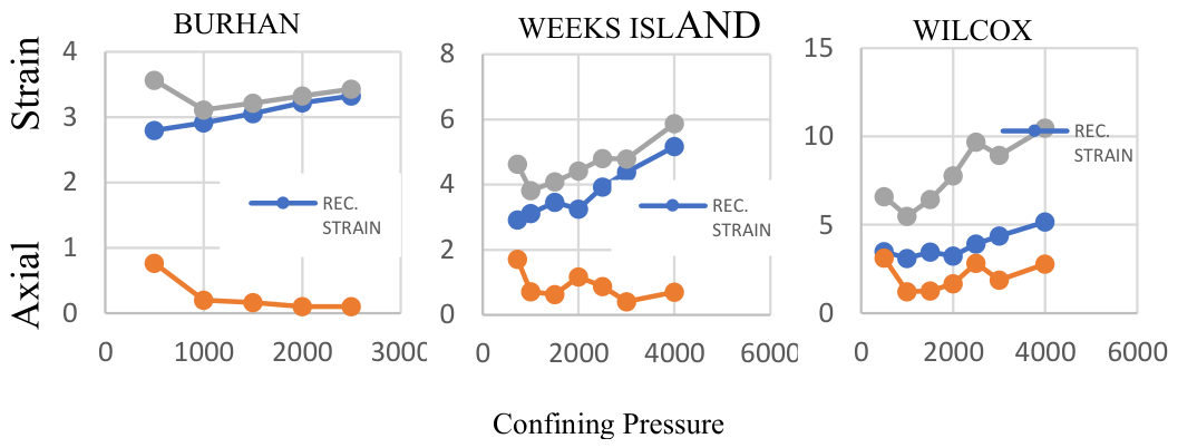
4.6. Recoverable Strain Plots
Figure 18 shows a plot of axial strain versus confining pressure for Group I. This plot is used to calculate amounts of irrecoverable, recoverable and total strain shown in Figure 17. The maximum amount of irrecoverable strain is always observed in the first ramp. The sample is exposed to a new stress path and therefore, has largest irrecoverable strain. All samples show large amounts of recoverable strain and small amounts of irrecoverable strain. The recoverable strain increases with each confining pressure cycle whereas the irrecoverable strain stays relatively constant. Irrecoverable strain is correlated with accumulated damage indicating that the increase in accumulated damage is approximately constant for all stages. The last ramp includes the strain to failure and therefore, has a larger amount of incremental strain than the other ramps.
Figure 17.
Shows a plot of confining pressure and axial strain to calculate irrecoverable, recoverable and total strain. All samples show that the recoverable strain increases with each confining pressure cycle and irrecoverable strain is constant.
Figure 17.
Shows a plot of confining pressure and axial strain to calculate irrecoverable, recoverable and total strain. All samples show that the recoverable strain increases with each confining pressure cycle and irrecoverable strain is constant.
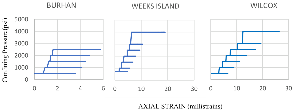
Figure 18.
shows a plot recoverable, irrecoverable and total strain versus confining pressure cycle. Total strain and recoverable strain increase at each step. Irrecoverable strain is largest for the initial ramp.
Figure 18.
shows a plot recoverable, irrecoverable and total strain versus confining pressure cycle. Total strain and recoverable strain increase at each step. Irrecoverable strain is largest for the initial ramp.
4.7. Mohr-Coulomb Plots
Mohr-coulomb plots for the three group I samples are shown in Figure 19. The BURHAN sample was terminated at a confining pressure ramp of 2500 psi due to limitations of the load cell.
Images
Figure 20 shows the microCT images for Weeks Island and Wilcox post failure. A limited number of conjugate fractures are evident. Figure 21 shows post-test 2D thin sections of WEEKS ISLAND. Thin section images for the other two samples are not available. Grain crushing is visible near the failure plane in Figure 21A.
4.8. Group 2 Samples
The second set of samples are finer grained Mudrock samples. They show a significantly different AE response from the Group 1 samples. This set of samples has a lower number of AE detected events in each triaxial stage. Therefore, their AE response is plotted on a linear scale and binned to interpret some features.
4.9. Fountain Plots – Group 2
Summary fountain plots of the Group 2 samples are shown in Figure 22. In the last stage (4000 psi confining) the sample is taken to failure, the strain curves show a distinct change in direction after the PPD is reached indicating an increase in rate of damage.
4.10. Strain Ratio Versus Axial Strain Plot – Group 2
Figure 23 shows the summary plots of strain ratio versus axial strain for fine-grained materials. For NICH, it is not very different. The initial loading ramp has a visibly different pattern compared to the reload ramps for NIO (purple). The reload ramps all track each other in all other plots. The slope of the curve at 4000 psi confining, changes between a ratio of 0.4 and 0.5. On the ramp to failure (pink highest axial strain), the slope of the curve increases rapidly after crossing the PPD, i.e., the sample is accumulating damage more rapidly.
4.11. AE Versus Deviatoric Stress Plot – Group 2
Figure 24 shows a plot of binned AE versus deviatoric stress for the Group 2 samples. The peak of the curves moves towards lower deviatoric stress with an increase in confining pressure. The sample is taking more damage early in the reload curve with an increase in confining pressure. This behavior suggests a more diffuse failure mechanism involved in these types of samples.
4.12. AE Versus Strain Ratio – Group 2
Figure 25 shows plots of AE versus PR for NICH and NIO. These samples show different characteristics. All the figures have an change of slope between 0.4 and 0.5 strain ratio. The slope of AE events changes (decreases) between a strain ratio of 0.4 and 0.45 for the Group 2 samples. AE characteristics change significantly around strain ratio of 0.5. The PPD is the optimum point to begin unloading.
4.13. Irrecoverable and Recoverable Strain Plots - Group 2
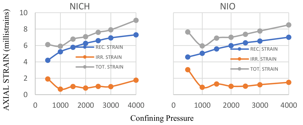
Figure 26 shows a plot of confining pressure to axial strain for Group 2 samples. This plot is used to calculate amounts of irrecoverable, recoverable and total strain. Maximum amount of irrecoverable strain is seen in the first ramp consistent with the larger strain. The sample is exposed to new stress path and therefore, has largest irrecoverable strain. Both samples show large amounts of recoverable strain and relatively small amounts of irrecoverable strain. The recoverable strain increases with each confining pressure cycle whereas the irrecoverable strain stays constant. The last ramp includes the ramp taken to failure and therefore, has a larger amount of incremental strain than the other ramps as can be seen in Figure 26. The mud rock samples have higher amounts of total strain compared to the coarser grained samples.
4.14. Axial Strain Versus Confining Pressure – Group 2
Irrecoverable strain and recoverable strain were calculated from Figure 26. Axial strain is zeroed at the beginning of each cycle. The recoverable strain increases in subsequent confining pressure cycles (Figure 26). The irrecoverable strain is constant for both samples. Irrecoverable strain is correlated with accumulated damage. The increase in accumulated damage is therefore constant for each of the stages.
Figure 27.
A Plot of recoverable, irrecoverable and total axial strain versus confining pressure for each stress cycle. The total strain increases in each successive ramp supported by increase in recoverable strain for mudrock samples. The irrecoverable strain is nearly constant after the initial loading.
Figure 27.
A Plot of recoverable, irrecoverable and total axial strain versus confining pressure for each stress cycle. The total strain increases in each successive ramp supported by increase in recoverable strain for mudrock samples. The irrecoverable strain is nearly constant after the initial loading.
4.15. Mohr-Coulomb Plots
Mohr-coulomb plots for NICH and NIO are shown in Figure 28. NICH shows higher cohesion than NIO. Friction angles for both samples are similar. NICH has a higher Young’s modulus and higher maximum compressive strength than NIO.
4.16. Micro-CT Images
Micro-CT images of the post-test NICH and NIO samples are shown in Figure 29. All samples had a brittle failure plane as can be seen in the CT pictures. Both samples show multiple conjugate fractures in addition to the major plane.
4.17. Thin Section Analysis
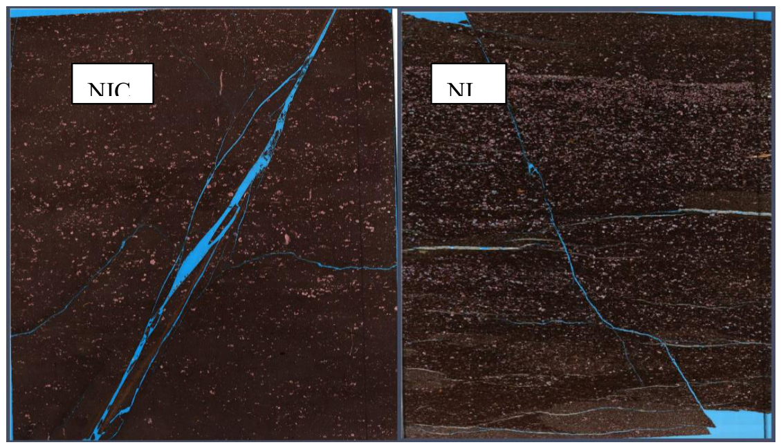
Figure 30 shows axial view of thin section images for NICH and NIO. A distinct failure plane is seen in this transmitted light image of the two samples. The parallel fractures seen in case of Figure 30. 2D thin section transmitted light image of NICH and NIO. A distinct failure plane is seen in both images. A small number of local failure planes are visible near the major failure plane. Transverse fractures in NIO were present prior to the test.
5. Discussion
Multi-stage tri-axial tests with acquisition of AE were performed on samples of five different formations. Samples were categorized into Group 1 and Group 2 samples based on their lithology. For all the samples a strain ratio of .5 was close to the optimum unloading point.
Counts of AE hits were determined to be a valid technique for assessing damage in MST tests. The AE behavior for the Group 1 samples followed expectations. The number of AE events had an approximately exponentially increasing relationship with increasing deviatoric stress. The reload ramps were all quieter than the initial loading ramp. An increase in the total number of AE events was seen after a strain ratio of 0.5, which supports that it is an optimum point to begin unloading in the MST test.
The Group 2 samples show similar trends in the MST plots such as fountain plots, axial strain ratio plots etc. The Group 2 samples behaved differently from Group 1 samples in terms of AE behavior. The number of AE events increased linearly with an increase in deviatoric stress and there were far fewer detected events. The slope of AE events was reduced at the PPD instead of increasing as seen in the Group 1. A shift in the peak of the binned AE curve towards lower deviatoric stress was also seen. The opposite behavior observed in quartz dominated samples. Using the PPD for the unloading point was also validated for this sample group.
In summary AE was used to validate choosing the unloading point for multistage triaxial tests.
Future work includes study of AE coda response under different loading conditions and as the sample approaches failure. The differing response of the Group 1 and Group 2 samples, indicated that they approach failure differently. Connection to Micro-CT images and thin section analysis is also identified as future work.
References
- Alsalman, M. E.; Myers, M. T.; Sharf-Aldin, M. H. Comparison of multistage and single-stage triaxial tests . Paper presented at the 49th U.S. Rock Mechanics/Geomechanics Symposium, San Francisco, CA, United States, 2015. [Google Scholar]
- Amitrano, D. Brittle–ductile transition and associated seismicity: Experimental and numerical studies and relationship with the b value. J. Geophys. Res. Solid Earth 2003, 108(B1), 2044. [Google Scholar]
- Anifrani, J. C.; Le Floc’h, C.; Sornette, D.; Souillard, B. Universal log-periodic correction to renormalization group scaling for rupture stress prediction from acoustic emissions. J. De Phys. I Fr. 1995, 5(6), 631–638. [Google Scholar] [CrossRef]
- Bak, P.; Tang, C.; Wiesenfeld, K. Self-organized criticality: An explanation of 1/f noise. Phys. Rev. Lett. 1987, 59(4), 381–384. [Google Scholar]
- Baud, P.; Klein, E.; Wong, T.-F. Compaction localization in porous sandstones: Spatial evolution of damage and acoustic emission activity. J. Struct. Geol. 2004, 26(4), 603–624. [Google Scholar] [CrossRef]
- Behringer, R. P.; Howell, D.; Kondic, L.; Tennakoon, S.; Veje, C. Predictability and granular materials. Phys. D. Nonlinear Phenom. 1999, 133(1–4), 1–17. [Google Scholar] [CrossRef]
- Bilal, A.; Myers, M. T.; Hathon, L. A. An investigation of static and dynamic data using multistage tri-axial test. Paper presented at the 50th U.S. Rock Mechanics/Geomechanics Symposium, Houston, TX, United States, 2016. [Google Scholar]
- Brantut, N.; Schubnel, A.; Guéguen, Y. Damage and rupture dynamics at the brittle–ductile transition: The case of gypsum. J. Geophys. Res. Solid Earth 116 2011, B01404. [Google Scholar]
- Burns, J.; Bradshaw, T.; Cole, P. Application of acoustic emission for quality assurance in capital projects. In Proceedings of the 7th Middle East Nondestructive Testing Conference & Exhibition (MENDT 2015), 2016. [Google Scholar]
- Carpinteri, A.; Lacidogna, G.; Niccolini, G. Critical behaviour in concrete structures and damage localization by acoustic emission. Key Eng. Mater. 312 2006, 305–310. [Google Scholar] [CrossRef]
- De Rubeis, V.; Hallgass, R.; Loreto, V.; Paladin, G.; Pietronero, L.; Tosi, P. Self-affine asperity model for earthquakes. Phys. Rev. Lett. 1996, 76(14), 2599–2602. [Google Scholar] [CrossRef]
- Fjaer, E.; Holt, R. M.; Horsrud, P.; Raaen, A. M.; Risnes, R. Petroleum related rock mechanics, 2nd ed.; Elsevier, 2008. [Google Scholar]
- Fortin, J.; Schubnel, A.; Guéguen, Y. Elastic wave velocities and permeability evolution during compaction of Bleurswiller sandstone. Int. J. Rock. Mech. Min. Sci. 2006, 42(7–8), 873–889. [Google Scholar]
- Ghasemi, S.; Khamehchiyan, M.; Taheri, A.; Nikudel, M. R.; Zalooli, A. Crack evolution in damage stress thresholds in different minerals of granite rock. Rock. Mech. Rock. Eng. 2020, 53(3), 1163–1178. [Google Scholar]
- Guo, T. Y.; Zhao, Q. Acoustic emission characteristics during the microcracking processes of granite, marble and sandstone under Mode I loading. Rock. Mech. Rock. Eng. 55 2022, 5467–5489. [Google Scholar] [CrossRef]
- Hidalgo, R. C.; Kun, F.; Herrmann, H. J. Fracture model with variable range of interaction. Phys. Rev. E 2002, 65(3), 032502. [Google Scholar] [CrossRef]
- Johansen, A.; Sornette, D. Critical ruptures. Eur. Phys. J. B 2000, 18(1), 163–181. [Google Scholar] [CrossRef]
- Kovari, K.; Tisa, A. Multiple failure state and strain-controlled triaxial testing. Rock. Mech. 1975, 7(1–2), 17–33. [Google Scholar]
- Lavrov, A. V.; Shkuratnik, V. L. Deformation- and fracture-induced acoustic emission in rocks. Acoust. Phys. 51 2005, Suppl. 1, S2–S11. [Google Scholar] [CrossRef]
- Li, C.; Nordlund, E. Experimental verification of the Kaiser effect in rocks. Rock. Mech. Rock. Eng. 1993, 26(4), 333–351. [Google Scholar] [CrossRef]
- Liakopoulou-Morris, F.; Main, I. G.; Crawford, B. R.; Smart, B. G. D. Microseismic properties of a homogeneous sandstone during fault nucleation and frictional sliding. Geophys. J. Int. 1994, 119(1), 219–230. [Google Scholar] [CrossRef]
- Liu, Y.; Meng, X. Dynamic multifractal characteristics of acoustic emission about composite samples with different stress loading and unloading conditions. Sci. Rep. 14 2024, 7533. [Google Scholar]
- Lockner, D. A. The role of acoustic emission in the study of rock fracture. Int. J. Rock. Mech. Min. Sci. Geomech. Abstr. 1993, 30(7), 883–899. [Google Scholar] [CrossRef]
- Lockner, D.; Byerlee, J. D. Acoustic emission and fault formation in rocks. In Proceedings of the First Conference on Acoustic Emission/Microseismic Activity in Geological Structures and Materials; Hardy, H. R., Leighton, W. F., Eds.; Trans Tech Publications, 1977; pp. 99–107. [Google Scholar]
- Main, I. G.; Meredith, P. G.; Jones, C. A reinterpretation of the precursory seismic b-value anomaly from fracture mechanics. Geophys. J. Int. 1989, 96(1), 131–138. [Google Scholar] [CrossRef]
- Michlmayr, G.; Cohen, D.; Or, D. Sources and characteristics of acoustic emissions from mechanically stressed geologic granular media: A review. Earth-Sci. Rev. 2012, 112(3–4), 97–114. [Google Scholar] [CrossRef]
- Mogi, K. Magnitude-frequency relation for elastic shocks accompanying fractures of various materials and some related problems in earthquakes. Bull. Earthq. Res. Inst. 40 1962, 831–853. [Google Scholar]
- Ohnaka, M.; Mogi, K. Frequency characteristics of acoustic emission in rocks under uniaxial compression and its relation to the fracturing process to failure. J. Geophys. Res. Solid Earth 1982, 87(B5), 3873–3884. [Google Scholar] [CrossRef]
- Pollock, A. A. Acoustic emission inspection. In Metals handbook; ASM International, 1989; Vol. 17, pp. 278–294. [Google Scholar]
- Read, M. D.; Ayling, M. R.; Meredith, P. G.; Murrell, S. A. F. Microcracking during triaxial deformation of porous rocks monitored by changes in rock physical properties, II. Pore volumometry and acoustic emission measurements on water-saturated rocks. Tectonophysics 1995, 245(3–4), 223–235. [Google Scholar] [CrossRef]
- Scholz, C. H. The frequency-magnitude relation of microfracturing in rock and its relation to earthquakes. Bull. Seismol. Soc. Am. 1968, 58(1), 399–415. [Google Scholar] [CrossRef]
- Scott, T. E.; Zeng, Z.-W.; Roegiers, J.-C. Acoustic emission imaging of induced asymmetrical hydraulic fractures. Paper presented at the 4th North American Rock Mechanics Symposium, Seattle, WA, United States, 2000, July. [Google Scholar]
- Stanchits, S.; Vinciguerra, S.; Dresen, G. Ultrasonic velocities, acoustic emission characteristics and crack damage of basalt and granite. Pure Appl. Geophys. 2006, 163(5–6), 975–994. [Google Scholar] [CrossRef]
- Sun, Y.; Yu, F.; Lv, J. Experimental study on acoustic emission characteristics of granite and sandstone under uniaxial compression. Geofluids 2023 2023, 2944871. [Google Scholar]
- Tordesillas, A. Force chain buckling, unjamming transitions and shear banding in dense granular assemblies. Philos. Mag. 2007, 87(32), 4987–5016. [Google Scholar] [CrossRef]
- Tordesillas, A.; Zhang, J.; Behringer, R. P. Buckling force chains in dense granular assemblies: Physical and numerical experiments. Geomech. Geoengin. 2009, 4(1), 3–16. [Google Scholar] [CrossRef]
- Wang, T.; Wang, L.; Xue, F.; Xue, M. Identification of crack development in granite under triaxial compression based on the acoustic emission signal. Int. J. Distrib. Sens. Netw. 2021, 17(1), 1–15. [Google Scholar] [CrossRef]
- Welker, P. R.; McNamara, S. Precursors of failure and weakening in a biaxial test. Granul. Matter 2011, 13(1), 93–105. [Google Scholar]
- Yabe, Y. Evolution of source characteristics of AE events during frictional sliding. Earth Plan. Space 2008, 60(4), e5–e8. [Google Scholar] [CrossRef]
- Youn, G. A.; Tonon, F. Multistage triaxial test on brittle rock. Int. J. Rock. Mech. Min. Sci. 2010, 47(5), 813–820. [Google Scholar] [CrossRef]
- Zang, A.; Wagner, F. C.; Stanchits, S.; Janssen, C.; Dresen, G. Fracture process zone in granite. J. Geophys. Res. Solid Earth 2000, 105(B10), 23651–23661. [Google Scholar] [CrossRef]
- Zhang, L.; Liu, G.; Wei, X.; Zhang, Y. Mechanical properties and acoustic emission evolution of water-bearing sandstone under triaxial conditions. Front. Earth Sci. 11 2023, 1212095. [Google Scholar] [CrossRef]
- Zhang, R.; Dai, F.; Gao, M. Z.; Xu, N. W.; Zhang, C. P. Fractal analysis of acoustic emission during uniaxial and triaxial loading of rock. Int. J. Rock. Mech. Min. Sci. 79 2015, 241–249. [Google Scholar] [CrossRef]
- Zhao, X.; Zhou, T.; Zhai, T.; Ju, Y.; Zhu, J. Experimental investigation on crack initiation and damage stresses of deep granite under triaxial compression using acoustic methods. J. Rock. Mech. Geotech. Eng. 2023, 15(11), 3071–3078. [Google Scholar] [CrossRef]
Figure 1.
The experimental setup for AE monitoring. A single AE sensor is attached to the bottom end cap. The average of the two measurements from LVDTS is used to measure axial strain. The average of the two measurements from a cantilever bridge is used to calculate the strains.
Figure 1.
The experimental setup for AE monitoring. A single AE sensor is attached to the bottom end cap. The average of the two measurements from LVDTS is used to measure axial strain. The average of the two measurements from a cantilever bridge is used to calculate the strains.
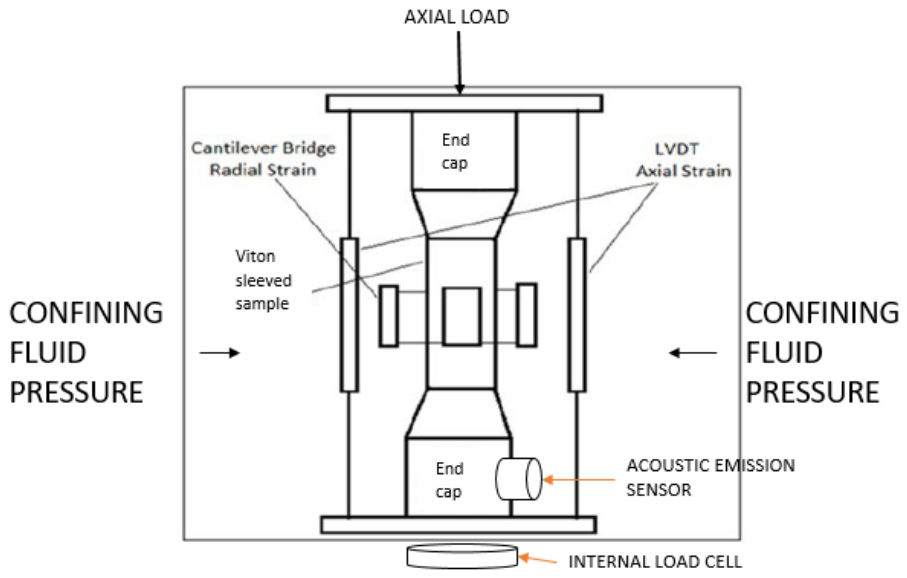
Figure 2.
A plot of axial strain versus volumetric strain. The PPD is identified as the point where the curve has a slope of zero. The sample is unloaded at this point in a multistage triaxial test.
Figure 2.
A plot of axial strain versus volumetric strain. The PPD is identified as the point where the curve has a slope of zero. The sample is unloaded at this point in a multistage triaxial test.
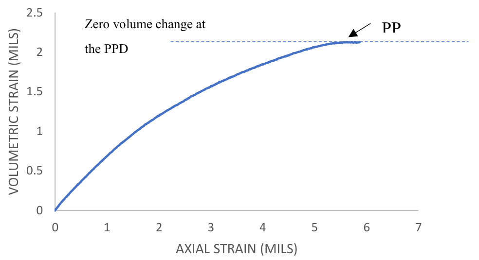
Figure 3.
An AE waveform with its attributes defined, threshold amplitude, rise time, duration, total number of counts and total energy.
Figure 3.
An AE waveform with its attributes defined, threshold amplitude, rise time, duration, total number of counts and total energy.
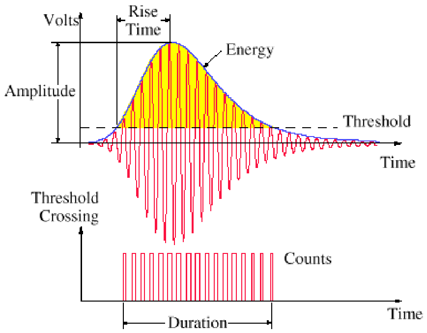
Figure 4.
Binning of AE data with respect to axial stress. The bin size of 0.25 axial strain was identified to minimize noise while retaining information. This bin size is used for all further analysis.
Figure 4.
Binning of AE data with respect to axial stress. The bin size of 0.25 axial strain was identified to minimize noise while retaining information. This bin size is used for all further analysis.
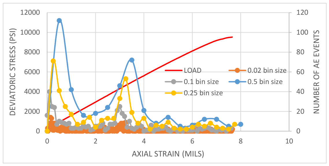
Figure 5.
Fountain plot data for a single stage of a MST measurement. The unloading point is the point of positive dilatancy. This is the stress at which the volume strain is zero. The strains are zeroed at the beginning of each loading cycle.
Figure 5.
Fountain plot data for a single stage of a MST measurement. The unloading point is the point of positive dilatancy. This is the stress at which the volume strain is zero. The strains are zeroed at the beginning of each loading cycle.
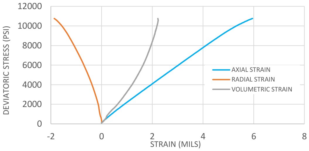
Figure 6.
This strain ratio versus axial strain plot. The radial strain increases rapidly at a strain ratio of .5.
Figure 6.
This strain ratio versus axial strain plot. The radial strain increases rapidly at a strain ratio of .5.
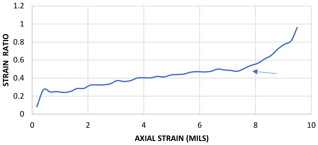
Figure 7.
A sample plot of deviatoric stress versus AE. This plot helps to understand the distribution of damage (assumed proportional to the number of AE events) with respect to applied deviatoric stress.
Figure 7.
A sample plot of deviatoric stress versus AE. This plot helps to understand the distribution of damage (assumed proportional to the number of AE events) with respect to applied deviatoric stress.
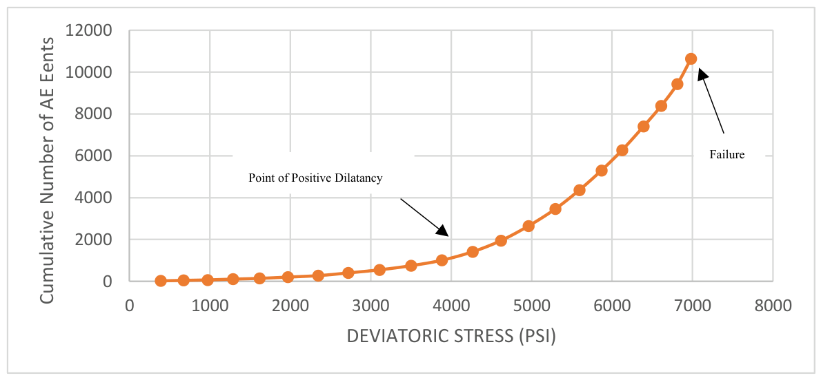
Figure 8.
A plot of deviatoric stress versus cumulative AE events at the same confining pressure. Multiple ramps are performed and the number of AE events were compared. They demonstrate the repeatability of a ramp.
Figure 8.
A plot of deviatoric stress versus cumulative AE events at the same confining pressure. Multiple ramps are performed and the number of AE events were compared. They demonstrate the repeatability of a ramp.
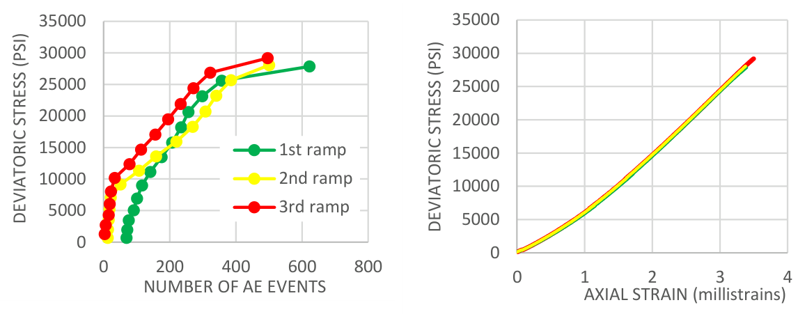
Figure 8.
The irrecoverable stain plot allows the amount of damage during each stress cycle of the multistage triaxial test to be determined.
Figure 8.
The irrecoverable stain plot allows the amount of damage during each stress cycle of the multistage triaxial test to be determined.
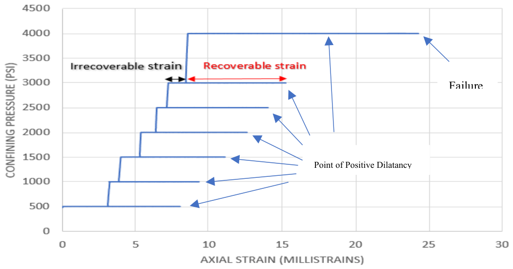
Figure 9.
Mohr Coulomb Diagram. This plot is used to map the yield surface, failure envelope and calculate friction angle and cohesion.
Figure 9.
Mohr Coulomb Diagram. This plot is used to map the yield surface, failure envelope and calculate friction angle and cohesion.
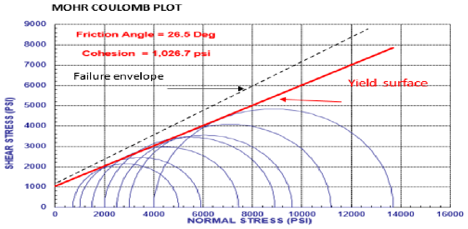
Figure 10.
Micro- CT image of a post-test rock sample. Failure plane can be clearly seen across the sample.
Figure 10.
Micro- CT image of a post-test rock sample. Failure plane can be clearly seen across the sample.
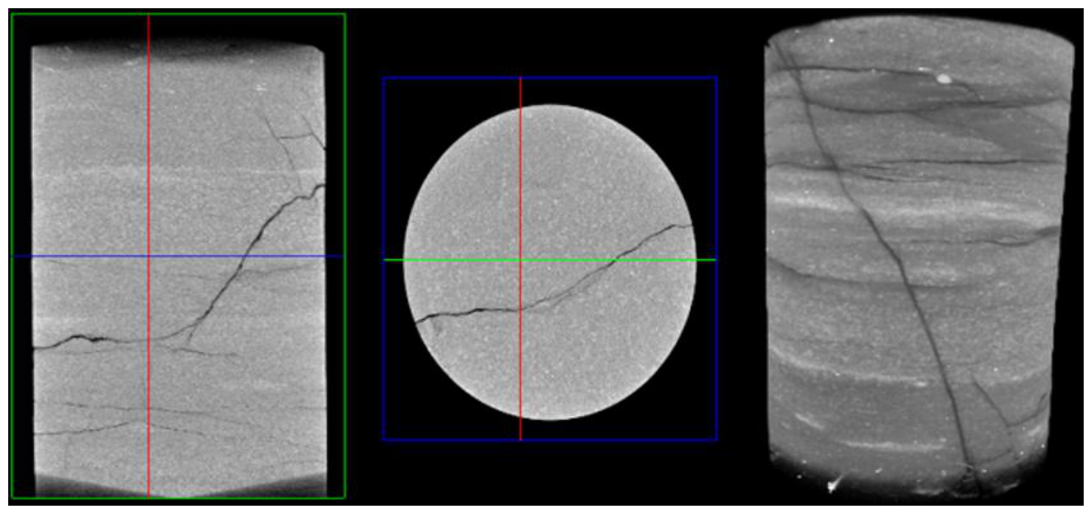
Figure 11.
A pre-measurement sample thin section image for Weeks Island. This is a coarse-grained weakly quartz cemented sandstone.
Figure 11.
A pre-measurement sample thin section image for Weeks Island. This is a coarse-grained weakly quartz cemented sandstone.
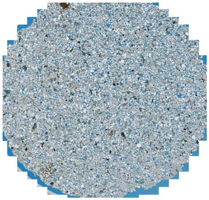
Figure 12.
Summary fountain plots of the Group 1 samples. These show the axial, volume and radial strains with varying confining stress.
Figure 12.
Summary fountain plots of the Group 1 samples. These show the axial, volume and radial strains with varying confining stress.
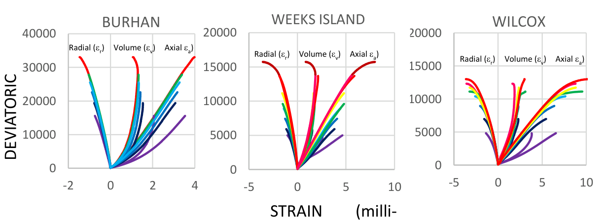
Figure 13.
Summary plot of strain ratio versus axial strain for WEEKS ISLAND, BURHAN and WILCOX. The slope of the curve is steeper after a strain ratio of 0.4-0.5, the sample is yielding rapidly.
Figure 13.
Summary plot of strain ratio versus axial strain for WEEKS ISLAND, BURHAN and WILCOX. The slope of the curve is steeper after a strain ratio of 0.4-0.5, the sample is yielding rapidly.
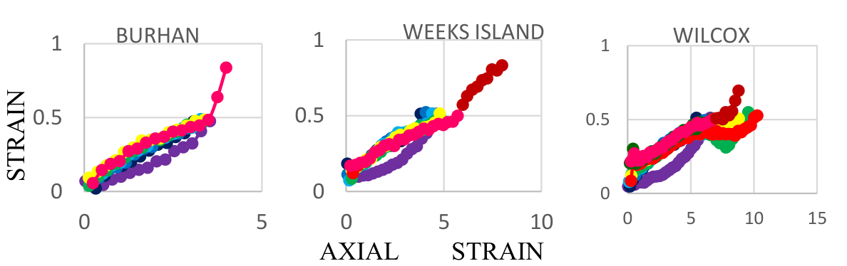
Figure 14.
Cross plot of cumulative AE and deviatoric stress for BURHAN WEEKS ISLAND, and WILCOX. Similar to Fig. 13. the different samples have a rapidly increasing cumulative number of AE events as the strain ratio approaches .5. Which is close to the point of maximum curvature.
Figure 14.
Cross plot of cumulative AE and deviatoric stress for BURHAN WEEKS ISLAND, and WILCOX. Similar to Fig. 13. the different samples have a rapidly increasing cumulative number of AE events as the strain ratio approaches .5. Which is close to the point of maximum curvature.
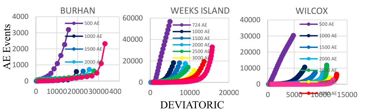
Figure 15.
A plot of AE versus Strain Ratio for the ramp to failure of the brittle samples. A rate of increase in the number of AE events is observed around a strain ratio of 0.5.
Figure 15.
A plot of AE versus Strain Ratio for the ramp to failure of the brittle samples. A rate of increase in the number of AE events is observed around a strain ratio of 0.5.
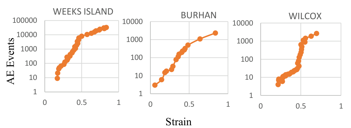
Figure 16.
shows deviatoric stress versus AE and Axial strain plots for the repeat ramp plots for Group I samples. The ramps repeat to within experimental error indicating a lack of significant damage.
Figure 16.
shows deviatoric stress versus AE and Axial strain plots for the repeat ramp plots for Group I samples. The ramps repeat to within experimental error indicating a lack of significant damage.
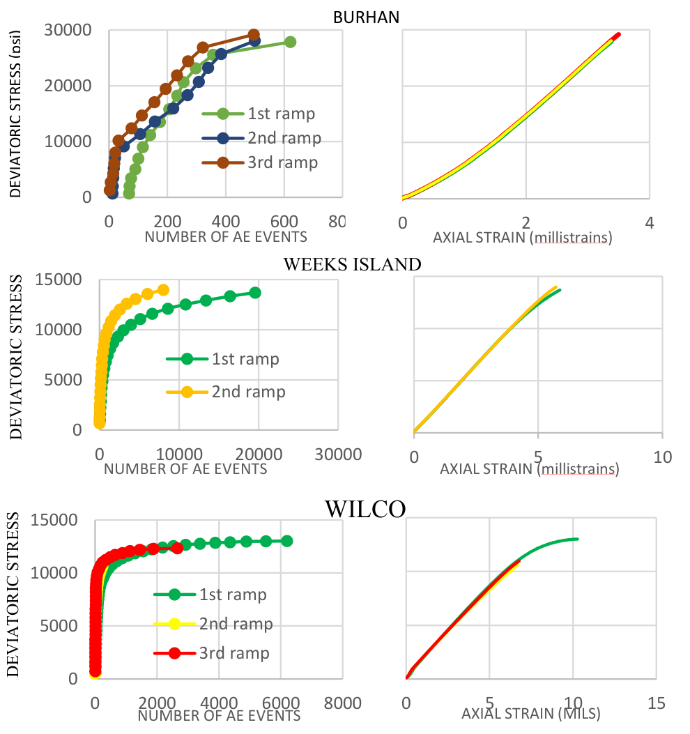
Figure 19.
Mohr-coulomb plots for the three samples.
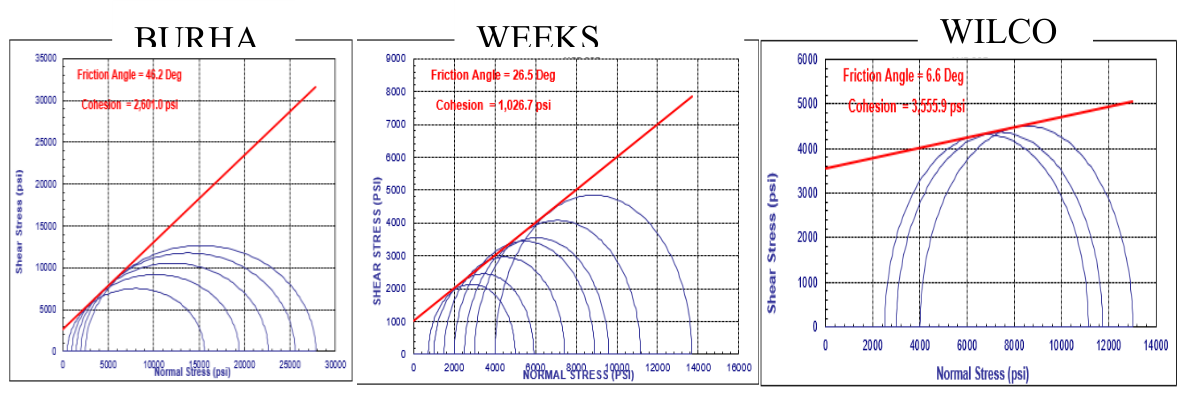
Figure 20.
Micro-CT images of all post-test samples for WEEKS ISLAND and WILCOX. BURHAN could not be failed due to load cell limitations. WEEKS ISLAND and WILCOX both show distinct failure planes.
Figure 20.
Micro-CT images of all post-test samples for WEEKS ISLAND and WILCOX. BURHAN could not be failed due to load cell limitations. WEEKS ISLAND and WILCOX both show distinct failure planes.
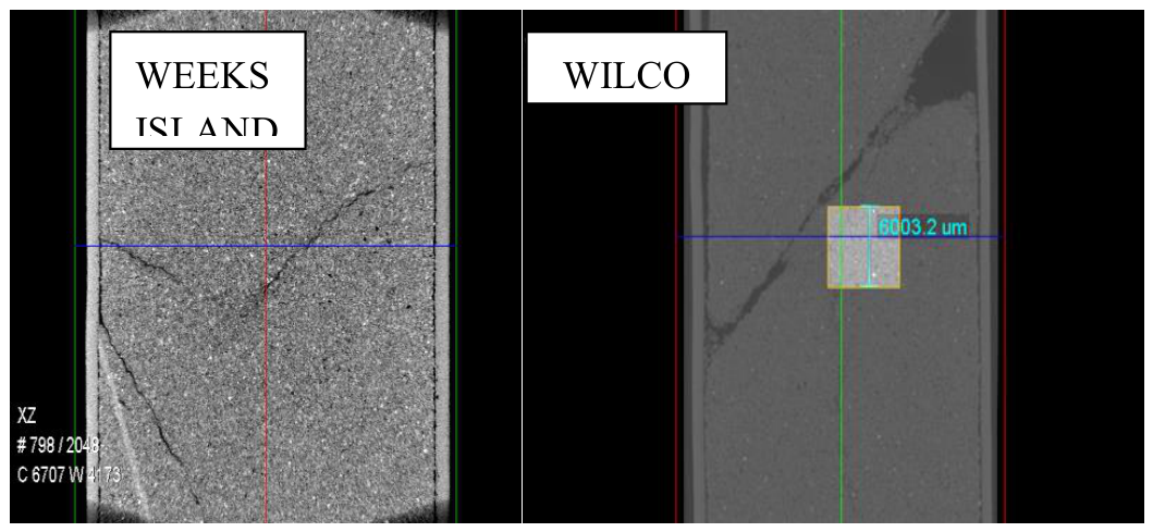
Figure 21.
Shows thin section images taken with transmitted light for WEEKS ISLAND. Grain crushing is visible near the failure plane in Fig 21(A).
Figure 21.
Shows thin section images taken with transmitted light for WEEKS ISLAND. Grain crushing is visible near the failure plane in Fig 21(A).
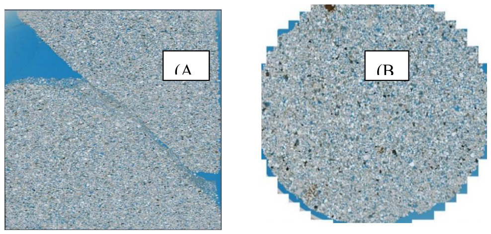
Figure 22.
Summary fountain plots of NICH and NIO. The samples are getting stiffer with increasing confining pressure. The initial ramp has a significantly lower Youngs modulus than subsequent higher confining stress ramps. NICH has a higher maximum compressive strength and higher Young’ modulus.
Figure 22.
Summary fountain plots of NICH and NIO. The samples are getting stiffer with increasing confining pressure. The initial ramp has a significantly lower Youngs modulus than subsequent higher confining stress ramps. NICH has a higher maximum compressive strength and higher Young’ modulus.
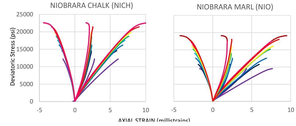
Figure 23.
Summary plot of PR versus axial strain for NICH and NIO. Reload stages track each other after the initial loading curve (purple). The sample is yielding rapidly after reaching a strain ratio of 0.4-0.5.
Figure 23.
Summary plot of PR versus axial strain for NICH and NIO. Reload stages track each other after the initial loading curve (purple). The sample is yielding rapidly after reaching a strain ratio of 0.4-0.5.
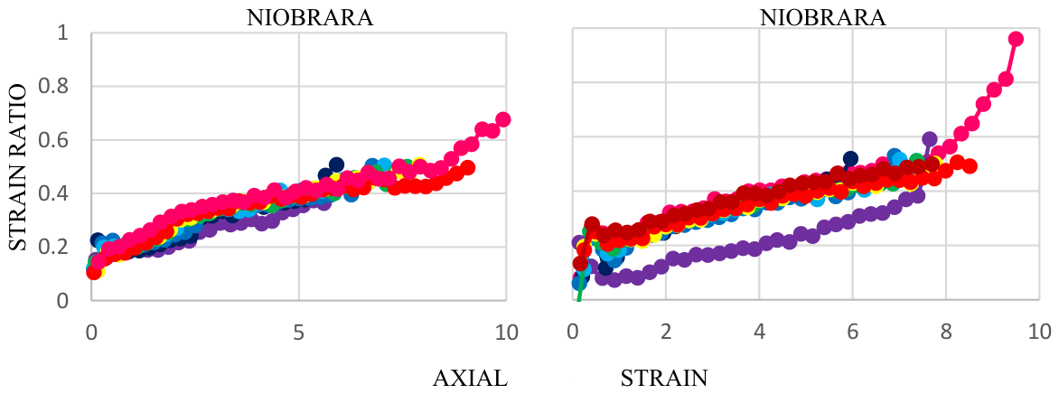
Figure 24.
A plot of binned AE data versus deviatoric stress for NICH and NIO. The peak of the curves moves towards lower stress at lower confining stress. This behavior is opposite to the group 1 samples.
Figure 24.
A plot of binned AE data versus deviatoric stress for NICH and NIO. The peak of the curves moves towards lower stress at lower confining stress. This behavior is opposite to the group 1 samples.
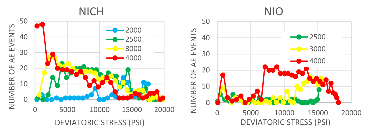
Figure 25.
A plot of AE versus strain ratio for the two Group 2 samples. Unlike the quartz dominated samples, a more linear increase is evident. An increase in number of AE events around a strain ratio of 0.5 is not visible. This suggests a more ductile and diffuse route to failure.
Figure 25.
A plot of AE versus strain ratio for the two Group 2 samples. Unlike the quartz dominated samples, a more linear increase is evident. An increase in number of AE events around a strain ratio of 0.5 is not visible. This suggests a more ductile and diffuse route to failure.
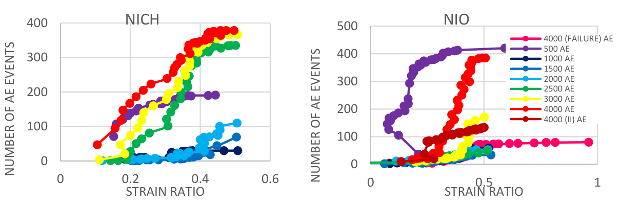
Figure 26.
A plot of confining pressure and axial strain to calculate irrecoverable, recoverable and total strain for mud rock samples. All plots show that the recoverable strain increases with each confining pressure cycle and irrecoverable strain i.
Figure 26.
A plot of confining pressure and axial strain to calculate irrecoverable, recoverable and total strain for mud rock samples. All plots show that the recoverable strain increases with each confining pressure cycle and irrecoverable strain i.
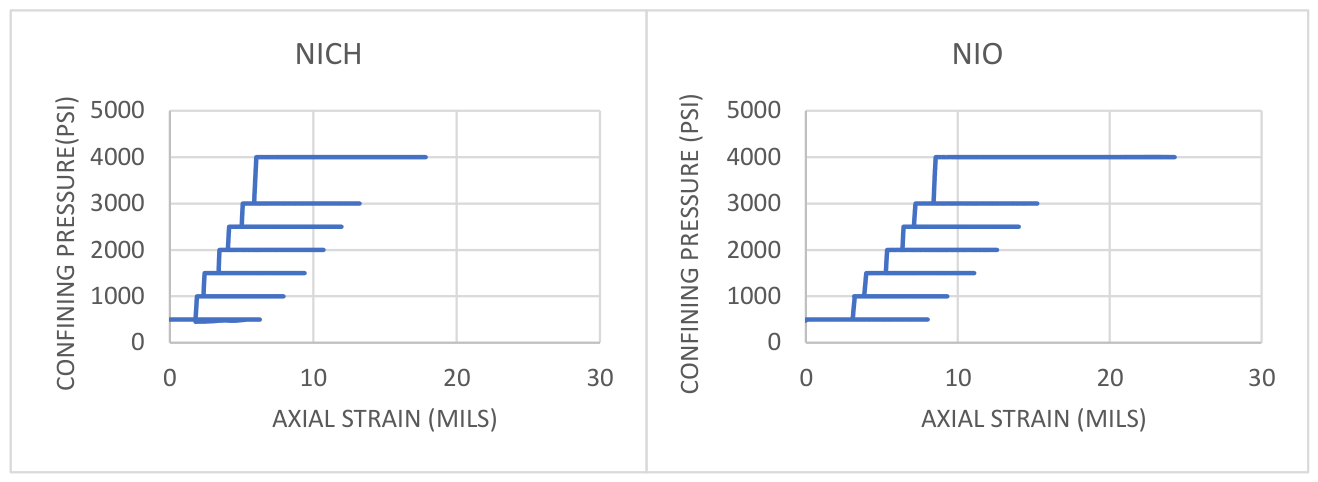
Figure 28.
Shows Mohr-coulomb plots for mud rock samples. NICH has a higher cohesion than NIO. Both samples have similar friction angles.
Figure 28.
Shows Mohr-coulomb plots for mud rock samples. NICH has a higher cohesion than NIO. Both samples have similar friction angles.
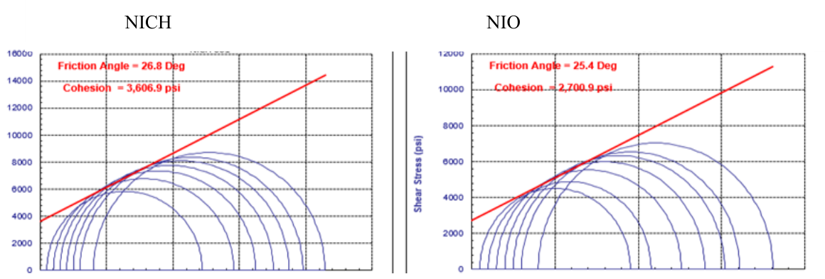
Figure 29.
Micro-CT images of the post-test Group II samples showing one major failure plane and other minor failure planes.
Figure 29.
Micro-CT images of the post-test Group II samples showing one major failure plane and other minor failure planes.
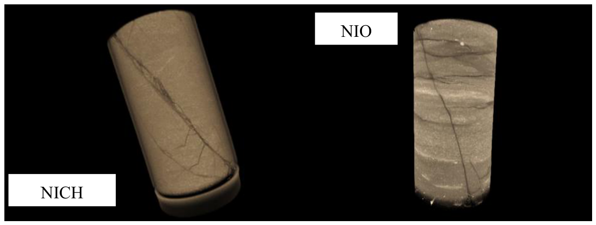
Figure 30.
2D thin section transmitted light image of NICH 001 (a) and NIO 001 (b). A distinct failure plane is seen in both images. A small number of conjugate fractures are visible near the major failure plane.
Figure 30.
2D thin section transmitted light image of NICH 001 (a) and NIO 001 (b). A distinct failure plane is seen in both images. A small number of conjugate fractures are visible near the major failure plane.
Disclaimer/Publisher’s Note: The statements, opinions and data contained in all publications are solely those of the individual author(s) and contributor(s) and not of MDPI and/or the editor(s). MDPI and/or the editor(s) disclaim responsibility for any injury to people or property resulting from any ideas, methods, instructions or products referred to in the content. |
© 2026 by the authors. Licensee MDPI, Basel, Switzerland. This article is an open access article distributed under the terms and conditions of the Creative Commons Attribution (CC BY) license (http://creativecommons.org/licenses/by/4.0/).
Copyright: This open access article is published under a Creative Commons CC BY 4.0 license, which permit the free download, distribution, and reuse, provided that the author and preprint are cited in any reuse.


