

Submitted:
25 June 2026
Posted:
26 June 2026
You are already at the latest version
Abstract
Offshore methane emissions are increasingly quantified using a range of observational approaches, yet reported estimates often exhibit substantial variability with limited evidence of convergence. This study examines the underlying causes of this divergence by focusing on how atmospheric transport and dispersion processes govern the relationship between measured concentrations and inferred emission rates. Across methods, calculated emission estimates depend on common assumptions regarding plume behaviour, including steady wind–plume coupling, near-Gaussian shaped dispersion, adequate mixing, and full plume observability. While these assumptions often hold under well-mixed terrestrial conditions, they are frequently violated in the marine boundary layer, which is characterised by stratification, vertical decoupling, and layered flow. To investigate this, an idealised dispersion model is used to compare three widely applied quantification approaches, Gaussian plume inversion, aircraft mass balance, and satellite-based methods, across representative offshore atmospheric regimes. By holding emissions constant and varying only atmospheric structure, the model isolates the role of transport processes in shaping inferred emissions. The results show that each method exhibits regime-dependent biases arising from distinct physical mechanisms. Gaussian methods are highly sensitive to plume alignment and may fail under lateral displacement; aircraft mass balance remains robust where the plume is fully sampled but becomes unreliable when sampling is incomplete; satellite methods consistently detect the plume but exhibit systematic bias where plume transport is decoupled from assumed wind speeds. Taken together, these results show that disagreement between offshore methane estimates can arise simply from changes in atmospheric regime. Under atmospheric conditions where standard transport assumptions are not satisfied, differences between estimates do not arise solely from measurement error, but from the way atmospheric structure affects how emissions are inferred from concentration measurements. Emission estimates derived from different methods are therefore only valid in specific atmospheric regimes, and their uncertainty cannot always be reduced through repeated measurements. This suggests that plume behaviour and its effect on sampling depend on both the method used and the atmospheric regime, and that emission estimates are only reliable where the underlying transport assumptions are satisfied, so convergence between emission estimates from different methods cannot be universally assumed under realistic offshore conditions.
Keywords:
offshore methane emissions
; marine boundary layer
; atmospheric inference
; non-convergence
; structural uncertainty
; plume dispersion
; stratification
; atmospheric transport
1. Introduction
Due to increasing requirements for quantifying, measuring, and reporting, interest in accurately measuring methane emissions from offshore oil and gas production facilities has increased in recent years [1,2,3,4,5]. Typically, methods infer methane emission rates from measured atmospheric concentrations and meteorological data; however, several assumptions are used within the modelling frameworks applied to calculate emissions [2,6,7,8,9]. Recent work has reviewed these methodologies, compared their performance, and highlighted uncertainties associated with each approach [10]. Despite growing interest, advances in method development, and improved observational capability, there remains a limited understanding of how well calculated emissions agree across different methodologies [11]. For example, emissions inferred using satellite, aircraft, and in situ methods can differ by orders of magnitude [10], and measurement-based estimates have been found to differ by up to 40% from inventory-based values [12].
While this study does not aim to compare existing methods, it instead addresses a more fundamental question. Specifically, it examines the atmospheric conditions under which concentration-based approaches can be used to infer physically valid methane emissions from offshore production facilities. The aim is to shift the focus from methodological performance towards a better understanding of the atmospheric processes that govern plume transport and dispersion in the marine boundary layer. One key question is whether transport assumptions derived from terrestrial boundary-layer conditions are universally valid offshore, and, if these assumptions are fundamentally violated, whether this invalidates calculated emissions.
Disagreement between top-down quantification methods is often attributed to uncertainty in meteorological measurements, methodological assumptions, or incomplete sampling [2,6,8]. While these factors are important, such uncertainty should, in principle, be reducible through improved measurement design and repeated observations. However, it is not intuitively obvious that increasing the number of measurements will resolve differences spanning orders of magnitude. This suggests that additional sources of uncertainty must be considered to improve method agreement.
The challenge in emissions quantification is the coupling of measurement and modelling, i.e. how emission rates are inferred from observations of atmospheric concentrations and meteorological conditions. Fundamentally, this depends on how the emitted plume interacts with the surrounding atmospheric flow field. In practice, atmospheric flow is shaped by boundary layer structure and turbulent mixing [13]. If these processes are not adequately parameterised, emission estimates may differ substantially, even when based on high-quality observational data.
To date, emission quantification methods have primarily been developed, tested, and tuned under onshore atmospheric conditions. These are typically relatively deep and well mixed, allowing rapid vertical and lateral dispersion of the plume. Under such conditions, near-surface wind measurements are generally representative of plume transport, and concentration measurements taken downwind of the source can be used to infer emission rates using simplified dispersion models such as Gaussian plume formulations [13,14,15]. Although these approaches rely on empirically derived parameters to describe dispersion, their underlying assumptions are often sufficiently satisfied to produce representative emission estimates under typical onshore conditions [13,16].
Offshore environments, however, differ from onshore in several key respects. The marine boundary layer is frequently characterised by shallow depth, persistent stratification, and reduced vertical mixing, particularly under stable or near-neutral conditions [17,18]. These features arise from the thermal properties of the ocean surface, as well as the influence of mesoscale and synoptic processes. As a result, plume transport is not always controlled by near-surface winds and may instead occur at different speeds and/or in different directions from the air being measured [17,18]. What remains unclear is whether methods developed and tuned using onshore observations are applicable offshore when the marine boundary layer is shallow or stratified.
In particular, quantification methods that assume alignment between plume transport and measured wind direction, such as Gaussian methods [6,7], may fail to accurately capture plume core concentrations, leading to systematic under- or overestimation of emission rates. Similarly, incomplete vertical mixing may result in only a fraction of the emitted plume being sampled, particularly when measurements are conducted at a single height or along a fixed transect [6,7,19]. Importantly, errors in quantification do not arise solely from measured quantities (e.g. instrument performance or data quality), but also from the underlying atmospheric conditions governing plume behaviour. These effects are consistent with observations of offshore methane emissions, where zero or very low emissions have been reported from operating facilities [6,8,9].
The increasing use of different methods to estimate offshore emissions has resulted in a wide range of reported values, yet nearly all approaches rely on assumptions that may not hold in a marine atmosphere. In this context, differences in reported emission estimates from relatively similar sources [6,8,9] are not necessarily caused by methodological inconsistency or poor experimental design. Rather, they may reflect physical constraints on plume behaviour imposed by the atmospheric environment. The marine boundary layer is often characterised by stratification, vertical decoupling, and layered flow—conditions that directly violate the assumptions embedded in standard inference approaches. This raises the possibility that disagreement between offshore methane estimates is not simply caused by measurement uncertainty, but is instead a consequence of applying these methods under conditions where their assumptions do not hold.
To address this, a simple modelling framework is developed to investigate the influence of atmospheric structure on emission quantification using typical methods. Three widely used approaches—Gaussian plume inversion, aircraft mass balance, and satellite-based methods—are evaluated under idealised offshore atmospheric regimes representing the dominant features of the marine boundary layer. By holding emissions constant and varying only atmospheric structure, the framework directly tests whether divergence between methods can arise from transport processes alone. Specifically, the study aims to: (1) identify assumptions shared across methods; (2) define representative offshore atmospheric regimes; and (3) quantify how calculated emissions vary across both method and atmospheric states.
Accordingly, this study does not seek to reproduce or validate specific field observations. Instead, it tests whether the dominant features of the marine boundary layer are sufficient to generate systematic differences between quantification approaches under controlled conditions. The objective is therefore to establish a physical mechanism for these differences, rather than to quantify their magnitude in any particular setting. In this context, the aim is not to reduce uncertainty to a bounded range, but to identify the conditions under which it becomes structurally embedded in the inference process itself.
2. Overview of Offshore Methane Quantification Approaches
A range of approaches have been adopted and then developed to quantify methane emissions from offshore oil and gas installations. These methods span spatial scales from individual component to regional atmospheric measurements and use a variety of measurement platforms, including in-situ sensors, mobile transects, aircraft, and satellite systems. Fundamentally, all approaches convert measured concentrations to emission rates by considering the gas’s atmospheric transport and are therefore sensitive to deviations from assumed plume behaviour. Despite differences in instrumentation, spatial resolution, and sampling strategy, the ability of each method to infer emissions depends on how accurately the transport of methane from source to sensor is modelled through advection and turbulent diffusion processes [20,21,22].
2.1. Downwind Dispersion and Gaussian Plume Approaches
Downwind dispersion approaches estimate emissions by measuring methane concentrations within a downwind plume at a distance from the source and applying a dispersion model to infer the emission rate. The Gaussian plume model and its extensions provide a widely used analytical framework for this purpose, relating source strength to downwind concentration distributions under idealised steady-state conditions [14,20,23,24].
Typically, methane concentration measurements are collected along a transect perpendicular to the plume, and the emission is then calculated using modelled dispersion behaviour. This approach relies on several assumptions, including steady wind conditions, homogeneous turbulence, Gaussian concentration structures, and consistent coupling between the plume and near-surface wind measurements [14,20,23,24]. These assumptions are mostly appropriate under well-mixed boundary-layer conditions.
2.2. Mass Balance Approaches
Mass balance approaches estimate emissions by combining integrated methane enhancements across a volume downwind with measurements of wind speed and direction [25]. This is typically implemented through transect measurements that capture the plume cross-section, with the total flux calculated as the product of excess concentration and transport velocity [8,26]. Mass balance methods require few assumptions about plume shape but it does assume plume coherence between vertical transects which retains dependence on atmospheric transport assumptions. These methods assume that the plume is fully captured within the measurement transect, i.e. have transects that measure zero-enhancement above and below the plume, and that the measured wind field accurately represents plume transport.
2.3. Aircraft and Satellite Remote Sensing
In terms of remote sensing, both aircraft and satellite-based methods use downward looking infrared spectrometers to observe column-integrated methane concentrations over spatial domains with emissions calculated from the total plume column mass, the length of the observed plume and wind speed. Aircraft platforms can be used to observe emissions from single facilities and detect plume down to ~5 kg CH4 h-1 [27,28]. There are two main types of satellite: earth observation and site-specific targeting satellites. Earth observation platforms observe methane enhancements over broad areas, e.g. Sentinel-2 has a swath width of 290 km, and a detection limit of is ~1400 kg CH4 h−1 ± 50% [29,30], while site-specific targeting systems, e.g. GHGSat, has a spatial resolution of 25 m and can ~200 kg CH4 h−1 ± 13% [2,31,32].
2.4. Common Structure Across Approaches
Despite their differences, the approaches described above share a common dependency on atmospheric transport and dispersion. Each method infers an emission by assuming a relationship between plume behaviour and the surrounding wind fields. All of these approaches assume the physical processes governing plume transport are sufficiently well understood and accurately represented.
Emissions reported by offshore measurement studies of similar sources show differences in emissions. In the Gulf of Mexico, average emissions of 25 kg CH4 h-1 were reported from 54 fixed leg platforms using downwind methods, 58 kg CH4 h-1 from 56 platforms using mass balance methods and 4930 kg CH4 h-1 from 151 platforms using remote sensing aircraft methods [6,8,9]. These differences suggests that boundary-layer processes such as stratification and decoupling could significantly affect plume structure and sampling completeness [10].
Accordingly, the comparison of offshore methane quantification approaches is less a question of methodological performance than of the models’ sensitivity to atmospheric transport. Understanding this sensitivity is essential for identifying the conditions under which quantification is valid and those under which it is fundamentally wrong.
3. Atmospheric Regime Framework
The marine boundary layer (MBL) provides the physical environment governing offshore plume transport. Its structure is highly variable and often differs from the terrestrial boundary layer, meaning that the assumptions underlying many quantification methods may not hold offshore. A defining feature of the MBL is its tendency toward vertical stratification. Unlike terrestrial boundary layers driven by diurnal heating, the MBL is influenced by air–sea temperature contrasts, cloud processes, and large-scale atmospheric dynamics [33,34,35]. These factors frequently produce stable or weakly mixed conditions, limiting vertical exchange.
3.1. Vertical Decoupling
Under many offshore conditions, the boundary layer becomes vertically decoupled. In these cases, the surface layer becomes dynamically separated from the air above. This can arise through cloud-top radiative processes or reduced turbulence [36,37]. The result is a layered structure in which different parts of the boundary layer exhibit distinct wind speeds and directions. Plumes emitted into such environments may become trapped within a particular layer and be transported independently of near-surface wind measurements.
3.2. Reduced Vertical Mixing
Stratification suppresses vertical mixing, confining plumes to narrow vertical regions. Rather than dispersing throughout the boundary layer, emissions remain concentrated within a limited height range. This produces strong vertical gradients in concentration, such that small differences in sampling height can lead to large differences in observed concentration [33].
3.3. Lateral Displacement and Shear
3.4. Implications for Plume Behaviour
These processes lead to several key characteristics: plumes may be vertically confined; plume position may be laterally shifted; and transport may occur in elevated layers. These effects are not considered in current quantification methods and could influence inferred emissions. To investigate how atmospheric regimes could affect emission quantification, three offshore atmospheric regimes were defined to represent MBL structures likely to be encountered during offshore methane measurements. These regimes reflect differences in boundary layer depth, vertical mixing, and coupling between atmospheric layers, which are known to influence plume transport and detectability. Atmospheric regimes are defined quantitatively using standard micrometeorological parameters, including boundary layer depth (), Monin–Obukhov stability (), and bulk Richardson number (), allowing direct comparison with observed marine boundary layer conditions.
The three offshore regimes therefore represent a progression from well-mixed to highly structured atmospheric conditions (Figure 1):
- Marine neutral deep: well-mixed, single-layer flow defined by near-neutral stability (|z/L| < 0.1), low Richardson number (RiB < 0.1), and a deep mixed layer (zi > 500 m), ensuring vertically coherent turbulence and strong wind–plume coupling.
- Marine neutral shallow: vertically confined but still coupled characterised by shallow boundary layers (zi ~ 102 m) and weakly stable conditions (0 < |z/L| < 1, RiB ≈ 0.1 – 0.25), resulting in reduced turbulence intensity and vertically constrained plume dispersion.
- Marine stratified: layered and decoupled flow defined by stable stratification (|z/L| >> 1, RiB > 0.25) and suppressed turbulence (σw < 0.2 m s-1), leading to vertical decoupling, strong wind shear, and multi-layer flow.
The regimes defined here represent idealised but physically grounded classes of marine boundary layer behaviour, and while real atmospheric conditions span a continuum, these discrete regimes provide a useful framework for isolating dominant transport processes relevant to emission inference.
The emission source was placed at a height of 50 m above mean sea level, representing a typical working deck elevation for offshore production platforms, particularly in exposed or deepwater environments [5]. An emission rate of 88 kg h⁻¹ was used as a representative offshore source. This value is large enough to produce a well-defined plume across all methods, but not so large that detection is guaranteed under all atmospheric conditions, allowing the influence of boundary layer structure on emission inference to be isolated [38]. A constant wind speed of 15 m s⁻¹ was assumed at the plume height (50 m), representing a typical strong offshore wind condition. This choice ensures coherent plume transport and isolates the effects of atmospheric structure (e.g. stratification and boundary layer depth) on plume behaviour [11].
4. Modelling Framework
4.1. Gaussian Boat-Based
To simulate a boat-based survey, methane concentrations were calculated along a transect perpendicular to the wind direction for each offshore atmospheric regime, at specified downwind distances and at a height of 2 m above the ocean surface. The maximum concentration observed along each transect was then used as input to a Gaussian plume model, tuned for onshore quantification, to estimate the emission rate. The downwind distance of the transects ranged from 50 m to 500 m. In lieu of measured wind speeds, the wind speed used in the emission calculation was derived from a logarithmic wind profile. Assuming a wind speed of 15 m s⁻¹ at 50 m, this corresponds to approximately 11 m s⁻¹ at 2 m for a surface roughness length of z₀ = 0.0002 m.
Although a Gaussian-based framework is employed, regime-dependent modifications to turbulence structure and wind profiles introduce departures from classical Gaussian assumptions, allowing systematic failure modes of standard inference approaches to be explored. The framework therefore serves as a controlled baseline against which sensitivity to atmospheric structure can be assessed.
4.2. Aircraft Mass Balance
Following descriptions of reported mass balance surveys, aircraft typically circle platforms at distances of 2–7 km [19,26], completing between 7 and 20 transects [12,19,26] at altitudes ranging from approximately 45 m to 1300 m above sea level, with vertical spacing between transects of 11–100 m [8,26]. For modelling purposes, a representative survey configuration was adopted, consisting of a flight path 4.5 km downwind of the emission source, with 12 equally spaced transects between 50 m and 1250 m above sea level. Emissions were calculated by integrating the difference between upwind and downwind concentrations across the plume cross-section (width × height), multiplied by the local wind speed. Wind speeds were calculated at measurement heights using a logarithmic wind profile. If the upper or lower transect remained within the plume, the plume extent was assumed to reach the boundary layer top or the ocean surface, respectively.
A Monte Carlo framework was used to assess the sensitivity of aircraft mass balance emission estimates to variability in survey design. For each simulation, key sampling parameters were randomly selected within ranges representative of reported field studies, including downwind distance (2–7 km), number of transects (7–20), and vertical sampling extent (approximately 45–1300 m). Transect heights were distributed evenly between randomly selected minimum and maximum altitudes, and plume concentrations were sampled along each transect. Emissions were then estimated by integrating the crosswind concentration field across both lateral and vertical dimensions, weighted by wind speed derived from a logarithmic wind profile. This process was repeated 300 times for each atmospheric regime to generate a distribution of inferred emission rates.
4.3. Satellite-Based Approaches
Satellite-based emission estimates were simulated by exploiting the vertically integrated nature of remote sensing measurements. In this framework, methane concentrations were first modelled in three dimensions using a Gaussian plume formulation with regime-dependent modifications. These concentrations were then integrated vertically to produce a two-dimensional field of column-enhanced methane, analogous to satellite retrievals of column mixing ratios. For each simulated scene, the total column mass was obtained by integrating the enhanced concentrations across the plume footprint in both the crosswind and downwind directions.
Emissions were estimated by multiplying this integrated column mass by an assumed plume transport velocity, consistent with commonly applied satellite inversion approaches. A logarithmic wind profile was used to relate wind speed to height, with the satellite retrieval assumed to use wind speeds sampled at low altitude (randomly varied between 2 and 50 m) to reflect the typical reliance on near-surface or coarse-resolution meteorological data.
A Monte Carlo framework was implemented to represent variability in satellite sampling geometry and environmental conditions. For each atmospheric regime, multiple simulations were performed with randomised spatial domains and wind assumptions. The resulting distributions of inferred emissions demonstrate that, while the plume is consistently detectable in column-integrated measurements, errors arise primarily from mismatches between the assumed and actual plume transport velocity. These errors are amplified under stratified conditions, where vertical decoupling leads to systematic bias in emission estimates.
It is important to note that the modelling framework is intentionally idealised and is designed to isolate first-order physical mechanisms governing plume transport rather than to reproduce specific field conditions. As such, the results should be interpreted as mechanistic sensitivity experiments illustrating how violations of standard transport assumptions influence inferred emissions, rather than as quantitative predictions for any given site. These simplifications allow the isolation of first-order transport mechanisms while retaining physical consistency with observed marine boundary layer behaviour.
5. Results
5.1. Gaussian plume methods
Transect-based Gaussian plume sampling shows that offshore atmospheric structure strongly influences downwind methane concentrations (Figure 2). Under land-neutral deep boundary layer conditions, the plume remains symmetric and centred on the nominal centreline. The Gaussian inversion behaves as expected, with emission estimates converging to a constant value with increasing downwind distance (Figure 3). In contrast, offshore regimes introduce systematic deviations from this behaviour. In marine neutral and shallow boundary layers, enhanced vertical confinement leads to increased lateral spreading of the plume. Although the plume remains centred, peak concentrations are reduced, resulting in consistent underestimation of emissions when using standard Gaussian parameterisations (Figure 2). This bias is most pronounced at shorter downwind distances, where concentrations are further depleted by rapid lateral dispersion (Figure 3). The most significant departure occurs under stratified conditions, where the plume is displaced laterally due to shear and decoupling from the surface layer (Figure 2). In this regime, the sampling transect directly downwind, i.e. y = 0 m, fails to intersect the plume core, leading to near-zero measured concentrations despite ongoing emissions. This can yield negligible or highly unstable emission estimates (Figure 3).
Emission estimates inferred from transect-based Gaussian plume analysis varied significantly across atmospheric regimes. While estimates converged towards a single value under land-neutral conditions, offshore regimes exhibited persistent underestimation and, in stratified conditions, near-complete failure of detection when the plume was displaced from the sampling transect (Figure 3).
Under land-neutral deep conditions, emission estimates approach the true value at intermediate downwind distances, where the plume is well defined and sampling intersects the plume core. However, the estimates do not converge exactly to the true emission rate. This is because the method relies on simplified assumptions regarding plume structure and transport, including the use of a representative wind speed and an assumed dispersion profile. Small mismatches between the assumed and actual plume characteristics, as well as differences between plume transport speed and the wind speed used in the calculation, introduce systematic bias. As a result, even under conditions where the underlying assumptions are broadly satisfied, the method may produce consistent but slightly biased estimates rather than exact convergence to the true emission rate.
5.2. Aircraft Mass Balance
Results also show that aircraft mass balance quantification has a strong dependence on atmospheric structure and vertical coverage. Under land-neutral deep boundary layer conditions, the plume is well mixed vertically and can be observed across a broad range of altitudes, with clear symmetric transects centred on the nominal plume centreline (Figure 4). Marine neutral conditions are similar but have reduced peak concentrations, reflecting weaker vertical mixing and enhanced lateral dispersion. In both cases, the plume is sampled consistently across multiple heights, supporting robust emission quantification through cross-sectional integration.
Under shallow marine boundary layer conditions, the plume is strongly confined to the lowest altitudes and is only detected in the lowest transects (~50–150 m). At higher altitudes, concentrations above background are difficult to discern. Despite this limited vertical extent, the plume is still captured within the measurement domain, indicating that mass balance remains effective provided that sampling includes near-surface levels.
In contrast, stratified conditions result in a plume that is both vertically constrained and laterally displaced relative to the nominal centreline. As a result, no measurable signal is recorded across any of the sampled transects. This demonstrates that aircraft mass balance surveys can fail when plume structure deviates sufficiently from assumed alignment, particularly if the sampling volume does not intersect the plume.
The results of the Monte-Carlo analysis demonstrate clear differences in robustness between regimes (Figure 5). Under land-neutral and marine neutral deep conditions, estimated emissions cluster tightly around the true value (~88 kg h⁻¹), indicating stable and reliable performance of the mass balance approach. In contrast, marine shallow conditions exhibit a broader distribution and systematic underestimation, reflecting the limited vertical extent of the plume and dependence on low-altitude sampling. The greatest variability is observed under stratified conditions, where estimates frequently collapse toward zero. This occurs because the plume is laterally displaced and can fall entirely outside the sampled measurement volume, highlighting a fundamental limitation of the method under strongly stratified offshore conditions.
5.3. Satellite Methods
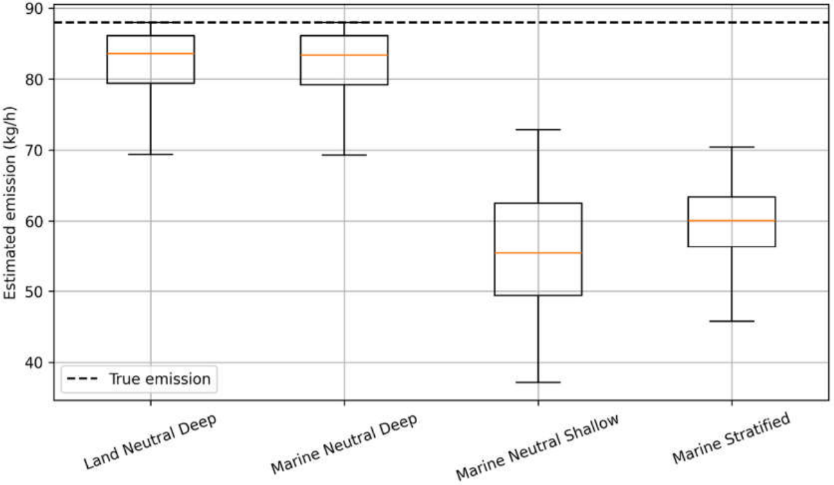
Satellite-based emission estimates exhibit systematic dependence on atmospheric regime, despite consistent detection of the plume in the column-integrated signal. Under land-neutral and marine neutral deep boundary layer conditions, inferred emissions cluster closely around the true value (~88 kg h⁻¹), with relatively narrow interquartile ranges (Figure 6). This indicates that, when plume transport is well mixed and aligned with near-surface winds, the use of a representative wind speed can provide a robust estimate of emission rate.
In contrast, offshore regimes characterised by reduced vertical mixing introduce increasing bias. Under shallow marine boundary layer conditions, estimated emissions are systematically lower, with median values between 50 and 65 kg h⁻¹ and increased spread. This reflects the confinement of the plume to lower altitudes, where wind speeds differ from those assumed in the retrieval, leading to underestimation.
An underestimate of emissions also occurs under stratified conditions, where median estimates are between 55 and 65 kg h⁻¹, and variability remains moderate. In this regime, the plume is vertically decoupled from the surface layer, and the assumption of near-surface wind speed introduces a consistent bias in the inferred emission. Unlike point or transect-based methods, the plume remains detectable in all cases; however, errors arise primarily from incorrect representation of wind speed rather than where the plume travels.
6. Discussion
6.1. Why Additional Measurements Do Not Guarantee Convergence
A common expectation in atmospheric measurement science is that increasing the volume, spatial coverage, or temporal resolution of observations will lead to improved agreement between independent estimates. This expectation is grounded in the assumption that uncertainty is primarily reducible through improved sampling, calibration, and instrumentation. However, the analysis presented above suggests that, in offshore environments, this assumption does not always hold.
Where uncertainty arises from violations of underlying transport and dispersion assumptions, additional measurements do not necessarily improve precision. Instead, the resulting variability may reflect a persistent feature of the system, caused by the interaction between plume behaviour and wind fields rather than limitations of the experimental setup.
In the marine boundary layer, mechanisms such as stratification, vertical decoupling, and shear introduce regime-dependent variability in plume transport. In these cases, plume structure differs between well-mixed and stratified conditions (Figure 1), affecting both the spatial distribution of emissions and detectability within a given sampling strategy. It follows that two measurements of the same source conducted with similar instruments and comparable sampling density in different atmospheric regimes may encounter different plume configurations, leading to different emission estimates.
A key example of this behaviour is wind–plume decoupling, where the effective transport pathway of a plume may diverge from the measured wind direction (Figure 2), particularly in stratified or layered flow regimes. Sampling strategies designed under the assumption of wind–plume alignment may therefore intersect the plume core in one instance and miss it in another, even under nominally similar meteorological conditions. Increasing the number of transects or extending sampling duration does not inherently resolve this issue if the underlying transport relationship remains misrepresented.
More generally, differences in measured concentrations reflect changes in atmospheric structure rather than random measurement noise, which can lead to incorrect emission estimates, particularly when only a limited number of measurements are available. In such cases, increasing the number of samples may result in a wider scatter of observations rather than converging toward a single value. Therefore, the range of calculated emissions reflects changes in atmospheric structure, rather than uncertainty around a single true value that could be reduced through additional measurements.
This explains why independent measurement campaigns may produce divergent results despite increased sampling effort and instrument density. Differences in calculated emissions may not only be caused by methodological inconsistency, but also differences in the atmospheric regimes encountered during measurement. As a result, increasing the amount of data does not necessarily lead to convergence when the underlying transport assumptions are not satisfied.
6.2. Reducible vs Structural Uncertainty in Offshore Contexts
The behaviour described above highlights the importance of distinguishing between reducible and structural components of uncertainty in offshore methane quantification.
Reducible uncertainty is caused by factors that can be addressed through improved measurement design or execution, including instrument precision and calibration, sampling density, spatial coverage, and data processing methods. These uncertainties are typically well characterised within atmospheric measurement methods and usually reduced through common approaches such as increased sampling frequency, improved calibration protocols, and enhanced sensor performance.
In contrast, structural uncertainty arises from limitations in methods’ underlying assumptions and reflects conditions where the relationship between observed concentration and emission rate cannot be reliably defined using the method as it stands. In the context of offshore methane measurement, structural uncertainty is associated with how valid transport and dispersion assumptions are under real offshore atmospheric conditions. Where actual plume behaviour deviates systematically from the assumptions used to relate concentration to emission rate, uncertainty does not only increase but is qualitatively altered. Under these conditions, uncertainty cannot be reduced through increased measurement density or precision alone.
Differentiating between these two forms of uncertainty is critical to understanding the emissions calculated. Reducible uncertainty can be addressed by improving the experiment, but structural uncertainty reflects a fundamental mismatch between the conceptual model and the physical reality of the atmosphere. In the latter case, additional data may drive down the uncertainty but does not necessarily improve the accuracy of inference. If measurements are made under conditions where transport assumptions are not satisfied, reducing reducible uncertainty may increase confidence in an emission estimate without improving its accuracy.
The marine boundary layer introduces structural uncertainty through its influence on plume transport. Processes such as stratification, vertical decoupling, and layered flow alter the relationship between emissions and measured concentrations in ways that are not captured by the transport models typically used to calculate offshore emissions. These effects are persistent and regime-dependent, rather than random or episodic.
Accordingly, offshore methane uncertainty is partly structural, arising from the inherent coupling between plume dynamics and atmospheric state. Under these conditions, uncertainty is not simply residual error, but arises from the way the inference method interacts with the atmosphere. Measurements can be made in all atmospheric regimes, but calculated emissions are only accurate where the underlying transport assumptions are satisfied. Failure to distinguish between reducible and structural uncertainty may lead to overconfidence in emission estimates. Including measurements made under conditions where underlying assumptions are not satisfied can obscure the interpretation of results and lead to systematic errors in inferred emission rates.
Structural uncertainty has direct implications for how offshore methane measurements are interpreted. These results show that emission estimates derived from atmospheric measurements are only conditionally valid, and that agreement between methods cannot be assumed under realistic offshore conditions. In this context, non-convergence is not necessarily due to measurement error, but can be an expected outcome of how plume behaviour changes across atmospheric regimes.
Where transport and dispersion assumptions are broadly satisfied, such as in well-mixed boundary layers, measurements can provide reliable and consistent emission estimates. However, when these assumptions are not satisfied, the link between measured concentration and emission rate breaks down, and the resulting estimates become difficult to interpret.
This means that claims of precision in offshore methane quantification need to account for the atmospheric conditions in which measurements are made. Emission estimates should not be treated as directly comparable without considering atmospheric regime. Differences between studies may therefore reflect differences in plume behaviour and sampling conditions, rather than differences in the underlying emissions.
This is particularly important for Gaussian, mass balance, and satellite approaches, all of which rely on assumptions about plume transport and structure. When these assumptions are not satisfied, differences in inferred emissions may arise from changes in plume position and observability, rather than real differences in emission rate.
More broadly, these results show that interpreting offshore methane measurements requires more than improving measurement accuracy. It requires understanding when the underlying assumptions hold and recognising when atmospheric structure limits what can be inferred. The consistent behaviour observed across multiple methods indicates that these effects are not specific to any one approach but arise from their shared dependence on atmospheric transport.
6.3. Interpretation of Large Reported Emissions
A key result of this work is that errors introduced by atmospheric structure are not symmetric. Across all three approaches, departures from idealised transport assumptions tend to reduce inferred emissions rather than increase them. Gaussian methods may miss the plume entirely if it is laterally displaced, aircraft mass balance returns very small values when the plume is not intercepted, and satellite approaches systematically underestimate emissions when plume transport is not aligned with the assumed wind speed.
This has direct implications for how large reported emissions should be interpreted. If atmospheric structure tends to reduce inferred emissions through incomplete sampling or incorrect transport assumptions, then large observed values are unlikely to arise from these effects alone. In practice, the same processes that lead to non-detection or underestimation—stratification, vertical confinement, and wind–plume decoupling—generally make emissions harder to detect, rather than easier to exaggerate.
One potential source of positive bias is incorrect representation of wind speed, particularly where the plume is transported in a layer with different velocity from that measured. This is most relevant for satellite approaches, and to a lesser extent for mass balance methods. However, realistic offshore wind profiles typically vary by factors of order two to three over the vertical range relevant to plume transport. As a result, wind mismatch alone is unlikely to generate large (order-of-magnitude) overestimates, although it may contribute to more moderate errors.
For substantial overestimation to occur within these methods, additional factors are required. These include double counting of plume mass, incorrect assumptions about plume extent, or errors in background subtraction. In aircraft mass balance, for example, overestimation may occur if a vertically confined plume is assumed to occupy a much larger portion of the boundary layer than it actually does. Even in these cases, the results presented here suggest that large positive bias is constrained and is unlikely to arise from atmospheric structure alone without significant methodological issues.
This does not mean that all large emission estimates are correct, but it does limit how they can be explained. Within the framework presented here, large values are more readily interpreted as either genuine high emissions or the result of specific methodological or operational artefacts, rather than arising naturally from atmospheric transport processes.
A related point is that the absence of a detectable plume does not imply low emissions. Under stratified conditions, plumes may be displaced vertically or laterally so that they are not sampled, even when emissions are substantial. This creates an asymmetry in interpretation: missed detections are common, but large overestimates are harder to produce through atmospheric effects alone.
Taken together, these results show that offshore emission estimates need to be interpreted within the limits set by atmospheric conditions. Atmospheric structure tends to reduce or obscure emissions, while errors associated with reducible uncertainty can increase estimates or create overconfidence in them. As a result, variability in offshore methane estimates is not symmetric, and estimates are more likely to be biased toward underestimation.
7. Conclusion
This study has examined how atmospheric structure constrains the inference of offshore methane emissions from atmospheric measurements, with a focus on the marine boundary layer. Although a range of observational approaches are used, they all rely on assumptions about how methane is transported and dispersed. The results here show that these assumptions are often not satisfied under typical offshore conditions.
As a result, differences between emission estimates cannot be explained solely by methodological differences or measurement uncertainty. Instead, they reflect how atmospheric structure influences plume behaviour. Processes such as stratification, vertical decoupling, and layered flow change how plumes are transported, dispersed, and sampled. This directly affects what is measured and how those measurements are interpreted. Divergence between estimates can therefore occur even when methods are applied correctly.
These results show that uncertainty in offshore methane quantification is not fully reducible. Part of the uncertainty is structural, arising from the interaction between plume behaviour and atmospheric conditions. In these cases, increasing the number of measurements may reduce noise but does not necessarily improve the accuracy of the inferred emission. Instead, it may reproduce the same variability under different atmospheric conditions.
This means that emission estimates derived from atmospheric measurements are only valid when the underlying transport assumptions are satisfied. Assessing these conditions is therefore essential for interpreting results. Without this, estimates may appear precise but still be incorrect.
Overall, this work shows that the limits of offshore methane inference are set not only by measurement capability, but also by atmospheric structure. Uncertainty cannot always be reduced through improved sampling alone, and may instead reflect a persistent feature of how emissions are observed in the marine boundary layer.
Funding
This research received no external funding. .
Institutional Review Board Statement
Not applicable.
Informed Consent Statement
Not applicable.
Data Availability Statement
No new data were created.
Acknowledgments
The author acknowledges the use of Microsoft Copilot to assist with manuscript preparation. Copilot was used for drafting, restructuring, and improving the clarity of the text. All scientific content, analysis, and conclusions are solely the responsibility of the author.
Conflicts of Interest
The author declares no conflicts of interest.
References
- Deshpande, S.; Collins, E.; Joynes, I.; O’Keeffe, R. Methane Emissions Measurement Insights from an Offshore Measurement, Monitoring, Reporting and Verification Study. Aust. Energy Prod. J. 2025, 65, EP24038. [Google Scholar] [CrossRef]
- MacLean, J.-P.W.; Girard, M.; Jervis, D.; Marshall, D.; McKeever, J.; Ramier, A.; Strupler, M.; Tarrant, E.; Young, D. Offshore Methane Detection and Quantification from Space Using Sun Glint Measurements with the GHGSat Constellation. Atmos. Meas. Tech. 2024, 17, 863–874. [Google Scholar] [CrossRef]
- OGMP Oil and Gas Methane Partnership 2.0—Key Benefits. Available online: https://www.ogmpartnership.org/key-benefits (accessed on 17 June 2025).
- EU The European Union. The New EU Methane Strategy. Available online: Https://Www.Europarl.Europa.Eu/Legislative-Train/Theme-a-European-Green-Deal/File-Methane-Strategy/09-2021 (accessed on 1/21/2020. 2021).
- Riddick, S.N.; Mbua, M.; Laughery, C.; Zimmerle, D.J. Assessing the Potential Impact of Fugitive Methane Emissions on Offshore Platform Safety. Safety 2025, 11, 115. [Google Scholar] [CrossRef]
- Yacovitch, T.I.; Daube, C.; Herndon, S.C. Methane Emissions from Offshore Oil and Gas Platforms in the Gulf of Mexico. Environ. Sci. Technol. 2020, 54, 3530–3538. [Google Scholar] [CrossRef] [PubMed]
- Riddick, S.N.; Mauzerall, D.L.; Celia, M.; Harris, N.R.P.; Allen, G.; Pitt, J.; Staunton-Sykes, J.; Forster, G.L.; Kang, M.; Lowry, D.; et al. Measuring Methane Emissions from Oil and Gas Platforms in the North Sea. Atmos. Chem. Phys. Discuss. 2019, 1–14. [Google Scholar] [CrossRef]
- Gorchov Negron, A.M.; Kort, E.A.; Chen, Y.; Brandt, A.R.; Smith, M.L.; Plant, G.; Ayasse, A.K.; Schwietzke, S.; Zavala-Araiza, D.; Hausman, C.; et al. Excess Methane Emissions from Shallow Water Platforms Elevate the Carbon Intensity of US Gulf of Mexico Oil and Gas Production. Proc. Natl. Acad. Sci. U.S.A. 2023, 120, e2215275120. [Google Scholar] [CrossRef] [PubMed]
- Ayasse, A.K.; Thorpe, A.K.; Cusworth, D.H.; Kort, E.A.; Negron, A.G.; Heckler, J.; Asner, G.; Duren, R.M. Methane Remote Sensing and Emission Quantification of Offshore Shallow Water Oil and Gas Platforms in the Gulf of Mexico. Environ. Res. Lett. 2022, 17, 084039. [Google Scholar] [CrossRef]
- Riddick, S.N.; Mbua, M.; Laughery, C.; Zimmerle, D.J. A Review of Offshore Methane Quantification Methodologies. Atmosphere 2025, 16, 626. [Google Scholar] [CrossRef]
- Riddick, S.N.; Mauzerall, D.L. Likely Substantial Underestimation of Reported Methane Emissions from United Kingdom Upstream Oil and Gas Activities. Energy Environ. Sci. 2023, 16, 295–304. [Google Scholar] [CrossRef]
- Foulds, A.; Allen, G.; Shaw, J.T.; Bateson, P.; Barker, P.A.; Huang, L.; Pitt, J.R.; Lee, J.D.; Wilde, S.E.; Dominutti, P.; et al. Quantification and Assessment of Methane Emissions from Offshore Oil and Gas Facilities on the Norwegian Continental Shelf. Atmos. Chem. Phys. 2022, 22, 4303–4322. [Google Scholar] [CrossRef]
- Seinfeld, J.H.; Pandis, S.N. Atmospheric Chemistry and Physics: From Air Pollution to Climate Change, Third edition.; John Wiley & Sons, Inc: Hoboken, New Jersey, 2016; ISBN 978-1-118-94740-1. [Google Scholar]
- Pasquill, F. Atmospheric Diffusion. By F. Pasquill. London (Van Nostrand Co.), 1962. Pp. Xii, 297; 60s. Q. J. R. Met. Soc. 1962, 88, 202–203. [Google Scholar] [CrossRef]
- Denmead, O.T. Approaches to Measuring Fluxes of Methane and Nitrous Oxide between Landscapes and the Atmosphere. Plant Soil 2008, 309, 5–24. [Google Scholar] [CrossRef]
- Edie, R.; Robertson, A.M.; Field, R.A.; Soltis, J.; Snare, D.A.; Zimmerle, D.; Bell, C.S.; Vaughn, T.L.; Murphy, S.M. Constraining the Accuracy of Flux Estimates Using OTM 33A. Atmos. Meas. Tech. 2020, 13, 341–353. [Google Scholar] [CrossRef]
- Dubey, R.R.; Mahato, B.; Yaghoobian, N. Effect of the Atmospheric Stability Condition on Buoyant Plume Dynamics. Phys. Fluids 2024, 36, 126615. [Google Scholar] [CrossRef]
- Hernandez-Jaramillo, D.C.; Kelaher, B.; Harrison, D.P. A Review of Plume Dispersion and Measurement Techniques Applicable to Marine Cloud Brightening. Front. Mar. Sci. 2025, 12, 1450175. [Google Scholar] [CrossRef]
- Khaleghi, A.; MacKay, K.; Darlington, A.; James, L.A.; Risk, D. Methane Emission Rate Estimates of Offshore Oil Platforms in Newfoundland and Labrador, Canada. Elem. Sci. Anth 2024, 12, 00025. [Google Scholar] [CrossRef]
- Stockie, J.M. The Mathematics of Atmospheric Dispersion Modeling. SIAM Rev. 2011, 53, 349–372. [Google Scholar] [CrossRef]
- Stull, R.B. Practical Meteorology: An Algebra-Based Survey of Atomspheric Science; UBC: Vancouver, 2017; ISBN 978-0-88865-283-6. [Google Scholar]
- Riddick, S. Fugitive Methane Emissions. In Cleaner Petroleum Production and Refining Technologies; Riazi, M.R., Yarranton, H.W., Eds.; Wiley, 2026; pp. 77–116. ISBN 978-1-394-20923-1. [Google Scholar]
- Pasquill, F.; Smith, F.B. Atmospheric Diffusion (3rd Edition); Ellis Horwood, (John Wiley & Sons): Chichester, 1983; Vol. 110. [Google Scholar]
- US EPA Industrial Source Complex (ISC3) Dispersion Model, Research Triangle Park, NC: U.S. Environmental Protection Agency. User’s Guide. EPA 454/B 95 003a (Vol. I) and EPA 454/B 95 003b (Vol. II). 1995. [PubMed]
- Conley, S.; Faloona, I.; Mehrotra, S.; Suard, M.; Lenschow, D.H.; Sweeney, C.; Herndon, S.; Schwietzke, S.; Pétron, G.; Pifer, J.; et al. Application of Gauss’s Theorem to Quantify Localized Surface Emissions from Airborne Measurements of Wind and Trace Gases. Atmos. Meas. Tech. 2017, 10, 3345–3358. [Google Scholar] [CrossRef]
- Pühl, M.; Roiger, A.; Fiehn, A.; Gorchov Negron, A.M.; Kort, E.A.; Schwietzke, S.; Pisso, I.; Foulds, A.; Lee, J.; France, J.L.; et al. Aircraft-Based Mass Balance Estimate of Methane Emissions from Offshore Gas Facilities in the Southern North Sea. Atmos. Chem. Phys. 2024, 24, 1005–1024. [Google Scholar] [CrossRef]
- Kunkel, W.M.; Carre-Burritt, A.E.; Aivazian, G.S.; Snow, N.C.; Harris, J.T.; Mueller, T.S.; Roos, P.A.; Thorpe, M.J. Extension of Methane Emission Rate Distribution for Permian Basin Oil and Gas Production Infrastructure by Aerial LiDAR. Environ. Sci. Technol. 2023, 57, 12234–12241. [Google Scholar] [CrossRef] [PubMed]
- Johnson, M.R.; Tyner, D.R.; Szekeres, A.J. Blinded Evaluation of Airborne Methane Source Detection Using Bridger Photonics LiDAR. Remote Sens. Environ. 2021, 259, 112418. [Google Scholar] [CrossRef]
- CDSE Copernicus Data Space Ecosystem. Sentinel-2 Documentation. Available online: https://documentation.dataspace.copernicus.eu/Data/SentinelMissions/Sentinel2.html (accessed on 1 June 2026).
- Schneising, O.; Buchwitz, M.; Reuter, M.; Bovensmann, H.; Burrows, J.P.; Borsdorff, T.; Deutscher, N.M.; Feist, D.G.; Griffith, D.W.T.; Hase, F.; et al. A Scientific Algorithm to Simultaneously Retrieve Carbon Monoxide and Methane from TROPOMI Onboard Sentinel-5 Precursor. Atmos. Meas. Tech. 2019, 12, 6771–6802. [Google Scholar] [CrossRef]
- Sherwin, E.D.; Chen, Y.; Ravikumar, A.P.; Brandt, A.R. Single-Blind Test of Airplane-Based Hyperspectral Methane Detection via Controlled Releases. Elem. Sci. Anthr. 2021, 9, 00063. [Google Scholar] [CrossRef]
- GHGSat Methane Emissions Monitoring. 2024. Available online: Https://Www.Ghgsat.Com/En/.
- Stull, R.B. (Ed.) An Introduction to Boundary Layer Meteorology; Springer Netherlands: Dordrecht, 1988; ISBN 978-90-277-2769-5. [Google Scholar]
- Garratt, J.R. The Atmospheric Boundary Layer; Cambridge atmospheric and space science series: Cambridge; Cambridge university press, 1994; ISBN 978-0-521-46745-2. [Google Scholar]
- Wood, R. Stratocumulus Clouds. Mon. Weather Rev. 2012, 140, 2373–2423. [Google Scholar] [CrossRef]
- Galewsky, J.; Jensen, M.P.; Delp, J. Marine Boundary Layer Decoupling and the Stable Isotopic Composition of Water Vapor. JGR Atmos. 2022, 127, e2021JD035470. [Google Scholar] [CrossRef]
- Albrecht, B.A.; Jensen, M.P.; Syrett, W.J. Marine Boundary Layer Structure and Fractional Cloudiness. J. Geophys. Res. 1995, 100, 14209–14222. [Google Scholar] [CrossRef]
- Riddick, S.N.; Mbua, M.; Laughery, C.; Zimmerle, D.J. Calculating Methane Emissions from Offshore Facilities Using Bottom-Up Methods. Eng 2025, 6, 199. [Google Scholar] [CrossRef]
Figure 1.
Simulated methane plume structure for four atmospheric regimes. Top row shows vertically integrated methane (column mass), representing satellite-like observations. Bottom row shows vertical cross-sections through the plume centreline. The dashed line in the top row indicates the nominal plume centreline (y=0), while the dotted line in the bottom row shows the source height (50 m). Stratified conditions exhibit vertical lifting and lateral displacement of the plume, resulting in strong sensitivity of observed concentrations to sampling position.
Figure 1.
Simulated methane plume structure for four atmospheric regimes. Top row shows vertically integrated methane (column mass), representing satellite-like observations. Bottom row shows vertical cross-sections through the plume centreline. The dashed line in the top row indicates the nominal plume centreline (y=0), while the dotted line in the bottom row shows the source height (50 m). Stratified conditions exhibit vertical lifting and lateral displacement of the plume, resulting in strong sensitivity of observed concentrations to sampling position.
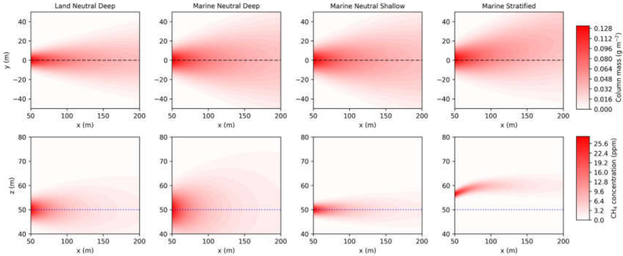
Figure 2.
Transect methane concentrations at 2 m height and 200 m downwind for four atmospheric regimes. The dashed line marks the assumed plume centreline. While land-neutral conditions produce symmetric plumes centred on the transect, offshore regimes show reduced peak concentrations and, under stratification, complete lateral displacement of the plume away from the sampling location, leading to failure of detection.
Figure 2.
Transect methane concentrations at 2 m height and 200 m downwind for four atmospheric regimes. The dashed line marks the assumed plume centreline. While land-neutral conditions produce symmetric plumes centred on the transect, offshore regimes show reduced peak concentrations and, under stratification, complete lateral displacement of the plume away from the sampling location, leading to failure of detection.
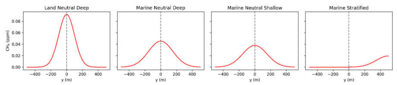
Figure 3.
Estimated emissions derived from Gaussian plume inversion as a function of downwind distance for each atmospheric regime. The dashed line indicates the true emission rate (88 kg h⁻¹). Under land-neutral conditions, estimates approach but do not exactly match the true emission rate due to small mismatches between assumed and actual plume properties.
Figure 3.
Estimated emissions derived from Gaussian plume inversion as a function of downwind distance for each atmospheric regime. The dashed line indicates the true emission rate (88 kg h⁻¹). Under land-neutral conditions, estimates approach but do not exactly match the true emission rate due to small mismatches between assumed and actual plume properties.
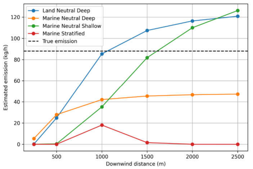
Figure 4.
Simulated crosswind methane concentration transects at 4.5 km downwind for aircraft mass balance sampling across four atmospheric regimes. Each column represents a different regime (Land Neutral Deep, Marine Neutral Deep, Marine Neutral Shallow, and Marine Stratified), and each row shows a horizontal transect at a specific sampling height between 50 m and ~1000 m above sea level. The dashed vertical line indicates the nominal plume centreline (y = 0).
Figure 4.
Simulated crosswind methane concentration transects at 4.5 km downwind for aircraft mass balance sampling across four atmospheric regimes. Each column represents a different regime (Land Neutral Deep, Marine Neutral Deep, Marine Neutral Shallow, and Marine Stratified), and each row shows a horizontal transect at a specific sampling height between 50 m and ~1000 m above sea level. The dashed vertical line indicates the nominal plume centreline (y = 0).
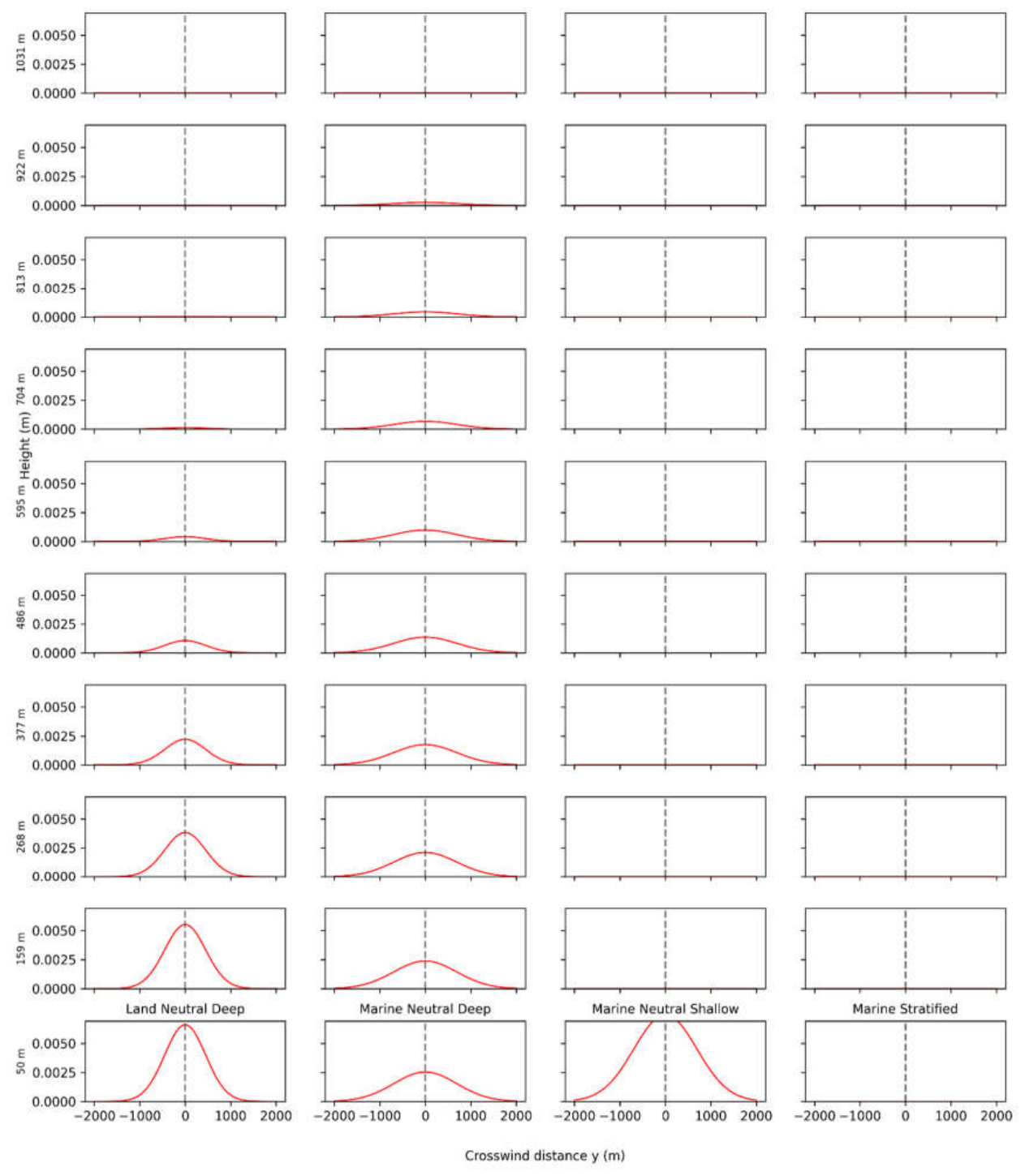
Figure 5.
Monte Carlo simulations of aircraft mass balance emission estimates across four atmospheric regimes. Each simulation randomly varies sampling distance, number of transects, and vertical coverage based on reported survey conditions. Box-and-whisker plots show the distribution of inferred emission rates, with the dashed line indicating the true emission (88 kg h⁻¹). Land-neutral conditions produce consistent and accurate estimates, while offshore regimes exhibit increasing variability. Stratified conditions show the greatest spread, including frequent underestimation, reflecting sensitivity to plume position relative to sampling geometry.
Figure 5.
Monte Carlo simulations of aircraft mass balance emission estimates across four atmospheric regimes. Each simulation randomly varies sampling distance, number of transects, and vertical coverage based on reported survey conditions. Box-and-whisker plots show the distribution of inferred emission rates, with the dashed line indicating the true emission (88 kg h⁻¹). Land-neutral conditions produce consistent and accurate estimates, while offshore regimes exhibit increasing variability. Stratified conditions show the greatest spread, including frequent underestimation, reflecting sensitivity to plume position relative to sampling geometry.
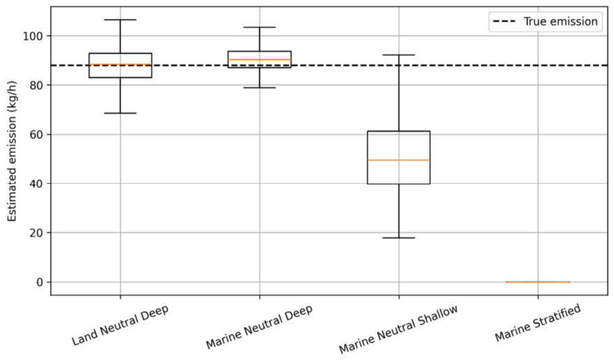
Figure 6.
Monte Carlo simulations of satellite-derived methane emission estimates for four atmospheric regimes. Emissions are inferred from vertically integrated plume mass using an assumed near-surface wind speed, with 300 simulations per regime representing variability in sampling conditions. Box-and-whisker plots show the distribution of inferred emissions, with the dashed line indicating the true value (88 kg h⁻¹).
Figure 6.
Monte Carlo simulations of satellite-derived methane emission estimates for four atmospheric regimes. Emissions are inferred from vertically integrated plume mass using an assumed near-surface wind speed, with 300 simulations per regime representing variability in sampling conditions. Box-and-whisker plots show the distribution of inferred emissions, with the dashed line indicating the true value (88 kg h⁻¹).
Disclaimer/Publisher’s Note: The statements, opinions and data contained in all publications are solely those of the individual author(s) and contributor(s) and not of MDPI and/or the editor(s). MDPI and/or the editor(s) disclaim responsibility for any injury to people or property resulting from any ideas, methods, instructions or products referred to in the content. |
© 2026 by the authors. Licensee MDPI, Basel, Switzerland. This article is an open access article distributed under the terms and conditions of the Creative Commons Attribution (CC BY) license (http://creativecommons.org/licenses/by/4.0/).
Copyright: This open access article is published under a Creative Commons CC BY 4.0 license, which permit the free download, distribution, and reuse, provided that the author and preprint are cited in any reuse.


