

Submitted:
25 June 2026
Posted:
26 June 2026
You are already at the latest version
Abstract
In this study, a decision-support model was proposed for evaluating orders in production environments. The developed model consisted of two stages. In the first stage, orders were classified by priority level. In the second stage, a mixed-integer programming model was developed using the classification output as input. In the first stage, orders were classified into priority classes based on criteria determined according to company priorities. For this purpose, Machine Learning (ML) models were developed using Random Forest (RF), Support Vector Machine (SVM), and K-Nearest Neighbors (KNN) algorithms. The classification structure covered both make-to-order (MTO) and make-to-stock (MTS) order types, and separate benefit and penalty coefficients were defined for each class. In the second stage, the resulting classification was translated into production decisions through a mathematical model that maximized total weighted benefit under capacity and budget constraints. The model generated an accept or reject decision for each MTO order. For MTS orders, quantities that could not be fulfilled due to constraints were postponed to subsequent periods. In addition, recommendations for reconsideration were provided for orders found to be infeasible following the second stage.
Keywords:
hybrid MTS/MTO
; order classification
; order management
; decision support models
; machine learning
1. Introduction
Increasing competitive conditions in the business world made it imperative for companies to manage their operations more efficiently, with lower costs, and in a more strategic manner. Changing consumer expectations, technological developments, and the widespread adoption of digitalization transformed the competitive environment into a more dynamic, complex, and unpredictable structure. In order to sustain their competitiveness in this environment, companies sought to gain a competitive advantage not only by offering quality products or services but also by adapting to change and capitalizing on new opportunities. Reducing non-value-adding costs, ensuring the effective use of existing resources, and maintaining environmental awareness and corporate responsibility provided companies with advantages in this regard. In addition, managing risks more effectively, building structures more resilient to uncertainty, and adopting flexible strategies capable of adapting to new opportunities became important elements of competitiveness.
One of the most critical problems within order management was the order acceptance decision. This problem required a systematic approach for evaluation. In hybrid systems, numerous qualitative and quantitative attributes exist, either interrelated or independent of one another. Therefore, identifying these attributes and subsequently using them effectively for order evaluation purposes constituted a critical and important issue. This decision also directly concerned and affected multiple departments, including sales or marketing, planning, production, and shipping. Furthermore, it carried strategic importance, as it influenced investment decisions, profitability, and customer satisfaction. This strategic approach and the associated decisions played a critical role in enabling companies to sustain their competitive advantage.
The decision support model developed in this study consisted of two stages designed to account for multiple factors. In the first stage, orders were grouped by classifying them into priority classes. Based on this classification, a mathematical model was developed that incorporated capacity, budget, and delivery constraints. In this way, orders that had been classified into priority classes and subjected to a comprehensive evaluation process were prepared for use in production.
The structure of this study is summarized as follows. Following the introduction, the second section presented studies in the literature related to order management. The third section presented the conceptual design of a decision support model developed based on the identified gap in the literature. In addition, the stages of the model were detailed, and the decision methods and implementation steps used at each stage were explained. The fourth section applied the developed model to real data and examined the resulting outputs. The final section evaluated the developed model in light of the application results and presented recommendations for future research related to the model.
2. Literature Review
When the make-to-order (MTO) and make-to-stock (MTS) production strategies were used together in production and planning processes, a hybrid MTS/MTO structure emerged. Although studies on pure MTO and pure MTS strategies had each been examined extensively in the literature, relatively few studies had addressed their combined use [1]. By using both MTS and MTO strategies together, the strengths of these methods could be combined and their weaknesses reduced. However, since this combination required taking more objectives and constraints into account simultaneously, the complexity of the resulting problems also increased. In practice, practitioners had long recognized the potential of hybrid MTS/MTO production systems, and interest in hybrid systems had recently increased [2]. Peeters and van Ooijen (2020) classified studies on different types of hybrid MTS/MTO production strategies found in the literature and re-evaluated the literature based on this classification [2]. The authors noted that the growth of the literature in this area had generally lacked a structured form, which made it difficult to review related studies and caused discussions on the topic to become complex. For this purpose, a classification study was conducted for different types of hybrid MTS/MTO production strategies. The authors also stated that the hybrid MTS/MTO production strategy was common in real industrial applications.
A hybrid production strategy referred to structures in which different production strategies were applied together within the same production system. The most commonly encountered form was the structure in which MTO and MTS strategies were used together. In these systems, some products were produced according to customer orders, while others were stocked based on demand forecasts [3]. The hybrid strategy sought a system that efficiently met customers' specific orders while offering a more favorable delivery date for the customer [4]. In addition to these objectives, it aimed to use existing capacity in the most efficient way. According to Kalantari et al. (2011), an appropriate combination of MTO and MTS could achieve both lower inventory and shorter lead times [5].
With the use of hybrid systems in production and planning processes, the decisions to be made and the problems addressed became even more complex. Some studies in the literature had focused on the problem of how production plans should be allocated to machines within the same production environment. For this purpose, various studies on capacity coordination had been conducted in the literature [6,7,8,9]. Scheduling, another important problem, became considerably more complex in hybrid structures. Some studies in the literature had focused on this problem [3,9,10,11,12]. A key challenge in such systems was determining the optimal location of this decoupling point. There were also several studies in the literature that focused on this problem [13].
In this context, the assumption that all orders should be fulfilled sometimes led to infeasible solutions in planning or scheduling problems. To prevent this situation, evaluation studies conducted for sales orders provided considerable value. Therefore, how orders would be evaluated before the master plan was prepared, along with which orders would be accepted or rejected, became an important problem. In the literature, these evaluation studies were addressed under the order acceptance/rejection problem. However, effective order acceptance/rejection decisions depended on the classification of orders according to specific characteristics. Therefore, this study presented a decision support model for the order acceptance/rejection problem.
Some studies in the literature presented general frameworks for the order acceptance/rejection problem and examined order acceptance/rejection decisions through staged models. Some of these stages involved qualitative evaluations, while others involved quantitative ones. Ashayeri and Selen (2001) developed a methodology for the order selection problem using a hierarchical production planning approach. This study aimed to maximize the total financial contribution of selected orders. The authors applied their methodology to a real hybrid MTS/MTO system [8]. Soman et al. (2004) presented a general framework for deciding on the key issues encountered in the use of a hybrid MTS/MTO system in the food industry [14]. In their study, the authors developed a three-stage decision model based on the literature. The authors concluded that the study made a valuable contribution both to the definition of the hybrid MTS/MTO production situation and to the managerial decision-making process in organizations. Due to the different strategies under which products were manufactured, a hybrid MTS/MTO production system required managerial activities considerably different from those required in pure MTO or pure MTS strategies. For example, during periods of low demand for MTO products, MTS products could be produced to fill capacity. However, in this case, questions such as how much inventory should be held needed to be answered. In addition, how the delivery date should be determined in a hybrid strategy constituted a separate problem. Manavizadeh et al. (2013) presented a decision support system for order acceptance/rejection using a mixed-model assembly line approach [15]. Order variety was the parameter examined in this study. The authors examined the problem in four steps. First, customers were prioritized according to their profit values. Then, the prices and delivery dates of orders that were not rejected were determined using a mathematical programming model. Subsequently, if the customer was not satisfied with the offered price and due date, renegotiation was recommended. Finally, if the negotiation resulted in an agreement, the order was accepted and added to the production schedule. In the model addressed by Rafiei and Rabbani (2012), products were classified into three categories: MTS, MTO, and hybrid MTS/MTO [9]. In this developed model, the authors presented a study on how capacity would be allocated among these three product types. The authors prioritized MTO orders according to four criteria: customer's profit contribution, customer's potential purchasing, orders' lot-sizes, and orders' purchasing range. MTS and hybrid MTS/MTO orders, on the other hand, were evaluated through pairwise comparisons based on three criteria: estimated contribution, reputation, and potential future sales. In the subsequent stage, the authors developed a mathematical model to determine lot sizes for MTS and hybrid MTS/MTO products. In the study, the initial capacity was allocated to MTO orders, while the remaining capacity was used for MTS and hybrid MTS/MTO products. Abedi and Zhu (2020) developed an order acceptance model for a system using a hybrid MTS/MTO strategy [1]. In the proposed model, a Mixed-Integer Linear Programming (MILP) model was developed to determine optimal order quantities based on resource availability. The model effectively reduced the risk of unreliable delivery dates arising from discrepancies between actual and available quantities. The model was compatible with systems involving both order-based and stock-based production. The model proposed in this study consisted of four stages. First, demands for MTO products were collected daily in batches. For MTS products, a forecasting model was applied to predict orders. In the second stage, a quantity-based Revenue Management approach was used to prioritize orders. In the third stage, an optimization model was developed to assess resource availability. In the final stage, orders deemed feasible based on resource availability were accepted, and the applicability of the developed approach was evaluated through two scenarios.
The hybrid MTS/MTO structure addressed in this study was illustrated in Figure 1. For a given product, production could be carried out specifically for a customer, or the product could be kept in stock based on forecasting studies. Accordingly, each order was held in the order pool as either an MTO order or an MTS order. Orders in this pool were evaluated during master planning using the structure described in detail in Section 3. Following the evaluation, orders considered feasible were included in the production schedule.
3. Materials and Methods
As a general approach in planning problems, the acceptance of all orders and their related processes was desired. However, in practice, some orders might need to be rejected. In real industrial environments, an order rejection decision could be made under various circumstances, such as low production capacity, high production costs, capacity constraints, certain machines not being active, a preference to produce specific products, or concerns about being unable to meet order commitments. When the relevant sales or marketing team wished to reject certain orders, the order selection problem aimed to maximize profit or minimize costs. Therefore, the processing of all orders could no longer be assumed in the planning problem, and an order acceptance problem thus emerged [16]. The objective of the order acceptance problem was to maximize the total benefit obtained from accepted orders. At the same time, rejecting an order also resulted in certain direct or indirect losses.
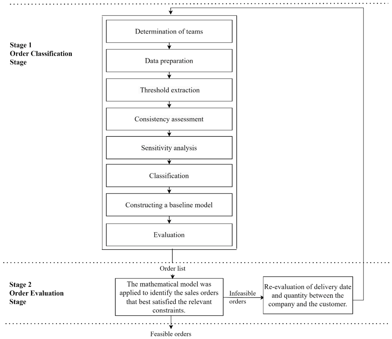
The conceptual design of the developed model was established by examining models in the literature. The objective of this model was to create a structure for evaluating sales orders and identifying feasible ones. The implementation stages of the model and the method used at each stage were summarized in Table 1 and illustrated in Figure 2.
In the order classification stage, the list of attributes was determined by decision-makers based on the literature or expert opinions. Data preparation was first carried out using these attributes. Using the prepared data, orders were classified into three priority classes through machine learning algorithms. Random Forest (RF), Support Vector Machine (SVM), and K-Nearest Neighbors (KNN) models, which were widely used in the literature for classification tasks, were employed for this purpose. In addition, the results obtained were compared across the algorithms. The objective of the classification process was not to determine the number of classes; these classes were predetermined, and orders were assigned to them accordingly. The classes used in this study were as follows:
- Class 1: Low priority
- Class 2: Normal priority
- Class 3: High priority
In the order evaluation stage, the set of orders determined in the first stage was used as input. In this stage, feasible sales orders were identified through the application of the mixed-integer programming model developed for this purpose.
In this developed model, both feasible and infeasible orders could be resubmitted to the model in batches. This model was also used during the master planning process, conducted on an annual or semi-annual basis. The model could be run separately for different periods. Furthermore, for infeasible orders, the model could be rerun following new mutual agreements reached with the customer regarding the delivery date or quantity.
Figure 2.
The framework of the developed model.
3.1. Listing of Selection Attributes
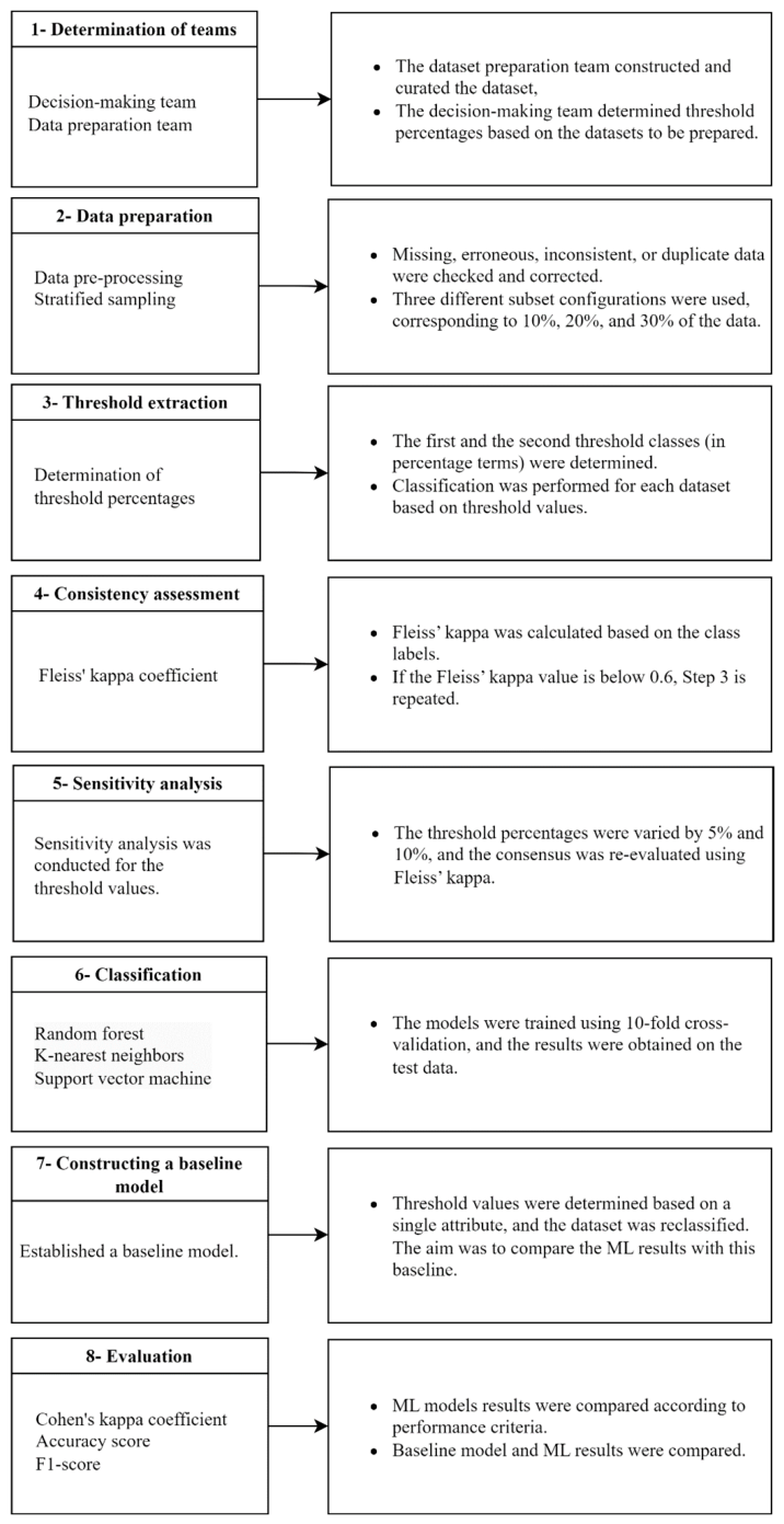
The implementation steps for order classification were illustrated in Figure 3. In the implementation, the teams were first determined. These teams could be organized as a "Data Preparation Team" and a "Decision-Making Team," or the same tasks could be carried out by a single team. In the second step, the relevant attributes for the classification process were determined. These attributes could be based on the literature or determined by the company according to expert opinion. In the third step, the data were cleaned and organized for processing. If the volume of data was large, various subsets were prepared. Threshold values were then determined based on the prepared data sets. After conducting consistency checks and sensitivity analyses, the ML models were run. In the final step, a baseline model was established to evaluate the performance of the ML models, and the results were compared.
The attributes used in this study were listed in Table 2. These attributes were defined as follows:
- Order quantity: This attribute referred to the total quantity within the relevant sales order. In this study, an order was considered an MTS order if it originated from a forecast, and an MTO order if it was customer-dependent.
- Order due date: For MTO orders, this attribute referred to the delivery date of the relevant sales order. For MTS orders, it referred to the forecasted delivery date of the corresponding forecast value. In this study, the delivery date was expressed in weeks.
- Order frequency: This attribute referred to the recurrence frequency of an order. It was calculated as a percentage over the determined period.
- Production cost: This attribute was considered at the order level and referred to the unit production cost of the relevant order.
The step-by-step details of the classification study illustrated in Figure 3 were as follows:
1. Determination of teams: To evaluate the data, two separate teams were established: a data preparation team and a decision-making team. The data preparation team carried out the necessary preliminary procedures to ensure that the data could be processed reliably. In this context, the data were examined for missing, erroneous, duplicate, or outlier values, and corrected if such values were found. In addition, attributes that were in text format were converted into numerical values. The decision-making team consisted of five members. These individuals were competent in evaluating sales orders. The expertise of the team members was considered sufficient and reliable for this evaluation.
2. Data preparation: The data preparation team checked for missing, erroneous, duplicate, or outlier values and corrected them where present. After the data were organized, they were divided into three different subsets of 10%, 20%, and 30% using the stratified sampling method. In this way, decision-makers were presented with subsets representing the distribution of the data set rather than the entire data set. This choice was made to enable decision-makers to analyze the data structure effectively and to reduce cognitive load. As the data size increased, agreement among decision-makers was expected to increase due to better representation of the data distribution. However, factors such as data heterogeneity and the ambiguity of class boundaries could cause this relationship to be non-linear. For this reason, the data subsets were prepared using the stratified sampling method.
3. Determination of threshold values: Decision-makers determined, as percentages, the first threshold separating the low and normal classes and the second threshold separating the normal and high classes for their respective orders. By using percentage-based thresholds instead of fixed threshold values, the comparability of orders at different scales was improved. This approach was more consistent with decision-makers' tendency to think in relative terms and strengthened the generalizability and interpretability of the model. Obtaining different classification results compared to absolute thresholds was an expected outcome and a natural consequence of scale dependency. Ultimately, class assignment was performed for the orders in each data subset using these determined threshold percentages, according to the following rule:
"If at least three of the relevant attributes are less than or equal to the first threshold, the order is assigned to Class 1; if at least three falls within the range between the first and second thresholds, it is assigned to Class 2; and if at least three are greater than or equal to the second threshold, it is assigned to Class 3."
4. Consistency assessment: Fleiss' kappa coefficient was calculated for each sample set. This calculation was performed and implemented in Python in accordance with the standard formulation of Fleiss' kappa. If the agreement value for any sample was found to be lower than 0.6, the decision-makers repeated Step 3. The purpose here was to achieve agreement among decision-makers. The variation in this agreement across different samples was intended to be assessed.
Fleiss' kappa is a coefficient that measures the level of agreement among multiple raters. The interpretation range commonly accepted in the literature is as follows:
- Value < 0,00: No agreement
- 0,00–0,20: Slight agreement
- 0,21–0,40: Fair agreement
- 0,41–0,60: Moderate agreement
- 0,61–0,80: Substantial agreement
- 0,81–1,00: Almost perfect agreement
5. Sensitivity analysis: To evaluate the sensitivity of the obtained threshold values to the data set, the entire analysis process was repeated on three independently constructed sample sets. The class assignments obtained from this process were then compared, and the agreement across the different samples was systematically examined. The reference sample set was the 30% sample. This variation was intended to be assessed using the 10% and 20% sample data.
In addition, to estimate confidence intervals for the threshold values, the determined thresholds were slightly altered, and class assignment was repeated. This reassignment was applied to the 30% sample data, and the resulting variation was evaluated. This method enhanced the statistical robustness of the findings and provided additional evidence for the stability and generalizability of the results. Large changes in threshold values were expected to alter the outcome. The purpose of this sensitivity analysis was to observe how small-scale changes affected the model.
6. Classification: Class assignment was performed for the entire data set using the determined threshold values. After the data were prepared, the accuracy and variance of the models were calculated using 10-fold cross-validation.
7. Constructing of the baseline model: A simple rule-based classification model was constructed. The classification results obtained from the baseline model were compared with the ML results. The purpose here was to observe the added value of the ML model. For example, if the RF model achieved an accuracy score of 93% while the baseline model achieved 75%, the added value of ML would be clearly demonstrated; however, if the baseline model also achieved an accuracy score of 90%, the necessity of ML would need to be questioned.
8. Evaluation: Cohen's kappa coefficient was used to test whether the difference between the baseline model and the ML models was statistically significant. In this test, if the probability value (p) was lower than 0.05, the difference between the models was considered statistically significant. In addition, the accuracy metric and the F1-score were used to evaluate the performance of the ML models.
Furthermore, two performance metrics were used to evaluate the ML classification results: the accuracy score and the F1-score.
Accuracy (AS) was the ratio of correct predictions to the total number of predictions.
The F1-score was another method used as a performance metric in the classification approach. It was calculated as follows. The Precision parameter gave the ratio of correctly predicted positive observations to the total predicted positives. The Recall parameter gave the ratio of correctly predicted positive observations among the actual positives. The F1-score was obtained from the harmonic mean of these two parameters.
TP referred to true positives, FP to false positives, and FN to false negatives.
Figure 3.
Application steps of the classification methodology.
3.2. Order Evaluation Stage
In the stage, a Mixed-Integer Linear Programming (MILP) model developed for the simultaneous optimization of the order selection decision was presented. The developed mathematical model was validated through various scenarios, and a sensitivity analysis was conducted on the coefficients used in the model. Furthermore, recommendations were provided for the reconsideration process between the company and the customer regarding orders found to be infeasible following the model.
Developed Mathematical Model
The mathematical model integrated both the MTS and MTO strategies and adopted a priority-class-based benefit structure. In the model, MTO orders were indivisible and could only be produced within their designated delivery periods and within a single period. Therefore, this characteristic required the corresponding decision variable to be defined in a binary form. MTS orders, on the other hand, were modelled using continuous variables that allowed for partial fulfilment, and a stock balance equation enabling inventory carryover between periods, and the tracking of cumulative demand backlog was integrated into the system. As a result, the selection of a greater number of MTO orders was made possible.
The assumptions of the model were as follows:
- All accepted orders were produced.
- Capacity overruns were not allowed.
- Capacity did not vary by product type.
- Capacity was defined on a periodic basis.
- An order could belong to only one class.
- MTO orders were indivisible, and production was carried out within a single period.
- MTO orders were produced in the period in which they arrived (no inventory was held).
- MTS orders were divisible.
- Inventory carryover was allowed for MTS orders.
- Capacity constraints were structured in a hierarchical manner based on a three-level priority classification (low, normal, and high priority), thereby mathematically ensuring that high-priority orders had prioritized access to available capacity.
- A holding cost was incurred for the amount of MTS inventory carried over to the subsequent period.
- Dates referred to the delivery date for MTO orders and the requirement date for MTS orders.
The notation used in the mathematical model was listed in Table 3. In this developed model, the objective function aimed to maximize the total benefit of accepted orders, weighted by priority-class-dependent benefit coefficients, while minimizing the penalty costs associated with inventory holding and demand backlog. The objective function of the model was defined as follows:
The terms in the objective function in Equation (1) corresponded, respectively, to the "MTO acceptance benefit, MTS production benefit, and MTO rejection penalty." The benefit and penalty coefficients were determined based on expert opinions.
Equation (2) represented the delivery date constraint for MTO orders. According to this equation, order i could only be produced in the period corresponding to its delivery date, and it could be accepted at most once in total. Equation (3) ensured that MTO orders were indivisible, and that MTO production could only take place within a single period as well.
Equation (4) ensured the inventory balance. If an MTS order could not be fully met in the corresponding period, the order was split. The unmet portion was carried over as a backlog to be produced in the subsequent period. In this equation, the parameter values for and needed to be provided as initial conditions. Furthermore, when multiple periods were used, initial conditions were used in place of and for the first period.
Equations (5), (6), and (7) represented the capacity constraints. Here, Class 3 received priority allocation from the available capacity, with the remainder used by Class 2. The portion remaining after that was then used by Class 1.
Equation (8) represented the budget constraint. This constraint defined the financial framework of production resources for each period and grounded the applicability of the model in a realistic operational context. The terms in this equation corresponded, respectively, to the "total production cost for accepted MTO orders, total production cost for the MTS order quantities to be produced, and total holding cost for MTS inventory carried over to the subsequent period." Equation (9) ensured that MTS production quantities were not concentrated on a single order.
Equation (10) defined the binary variable. Equation (11) defined the non-negative (positive) variables.
The following outputs were intended to be reported as model results:
- : Number of accepted MTO orders
- : Number of non-accepted MTO orders
- : Quantity of the MTS order produced in the period,
- : Unmet quantity of the MTS order for the period,
- : Remaining capacity quantity after the priority class in the period.

Table 3.
Notation used in the mathematical model.
| Indices | Description |
|---|---|
| i ϵ O | Set of MTO orders |
| j ϵ S | Set of MTS orders |
| c ϵ K | Priority classes (1;2; 3) |
| t ϵ L | Periods |
| Parameters | |
| w(c) | Benefit coefficient for MTO orders in priority class c |
| m(c) | Penalty coefficient for MTO orders in priority class c |
| d(i) | Delivery period of MTO order i |
| Qi | Quantity of MTO order i |
| a(i) | Unit production cost of MTO order i |
| F(j,t) | Planned requirement of MTS order j in period t |
| a'(j) | Unit production cost of MTS order j |
| h(j) | Unit holding cost per period for MTS order j |
| P(j,0) | Initial inventory of MTS order j (at the end of period 0) |
| w'(c) | Benefit coefficient for MTS orders in priority class c |
| CT(t) | Total capacity of period t |
| BD(t) | Budget of period t |
| Variables | |
| X(i,c,t) | 1, if MTO order i is produced and accepted in period t; 0, otherwise |
| X'(j,c,t) | Quantity of MTS order j produced in period t |
| P(j,t) | End-of-period inventory (surplus) of MTS order j in period t |
| N(j,t) | Cumulative backlog of MTS order j at the end of period t |
| R(c,t) | Remaining capacity in period t after consumption by priority class c |
Reconsideration of Infeasible Orders
After running the mathematical model, some orders might be obtained as infeasible. Instead of directly rejecting infeasible orders, several negotiation approaches could be applied. In this section, recommendations were provided for companies regarding various negotiation strategies. The relevant approaches were listed below:
- Delivery date modification: In order to reduce the delivery time of a specific order, a company might often need to reject or delay other orders. Rejecting or delaying orders could result in costs such as late delivery penalties or damage to the company's reputation. Therefore, an economic evaluation needed to be conducted between the benefit of reducing the delivery time of one order and the costs of rejecting or delaying other orders. When negotiating the delivery date, the company needed to minimize the probability of delay. This probability could be assessed by examining the company's operational process capacity, its past performance in meeting delivery dates, the availability of resources (machinery, materials, or labor), and the current workload in the production area [5].
- Order price modification: The company could shorten the delivery time by increasing the order price. Similarly, order prices could be reduced in exchange for extending delivery times [5].
- Order quantity modification: The entire quantity specified in an order might not be deliverable by the requested delivery date. In this case, the order quantity could be planned by splitting it across different periods. If earlier production was planned, a holding cost would be incurred. If holding costs were not desired, partial shipment would occur instead.
- Capacity modification: If the model under consideration involved multiple periods, infeasible orders could be planned for periods with lower capacity utilization. In this case, a change in the delivery date for the relevant order or orders would be required. If a date change was not feasible, overtime work could be implemented, or outsourcing could be considered. In this case, an increase in the operational cost of the order would occur. Therefore, the company needed to calculate the resulting additional costs and incorporate them into the order price [5].
If a change occurred in the parameters of infeasible orders following negotiations, the mathematical model needed to be rerun and the new results evaluated.
Validity Tests of the Mathematical Model
In this section, the solution quality, validity tests, and applicability of the proposed mixed-integer programming model were evaluated. The experiments were conducted on problem instances synthetically derived from real system parameters. The model was coded in the GAMS (General Algebraic Modelling System) software environment, and CPLEX was used as the solver. All tests were performed on a computer equipped with 8 GB of RAM and a 12th Generation Intel® Core™ i5-1235U processor (1.30 GHz).
The validity tests were designed in two stages. In the first stage, a small-scale verification scenario (S1) was run to confirm whether the model functioned correctly, and the resulting outputs were verified manually. In the second stage, problem instances systematically expanded in terms of the number of orders, period length, and initial inventory were tested to evaluate the scalability and practical applicability of the model. The scenarios used in the tests were presented in Table 4.
When Table 4 was examined, it was observed that the model achieved extremely short solution times for single-period problems. Starting from the verification scenario with 500 orders (S1, 0,031 s) up to the large-scale single-period scenario with 50,000 orders (S8, 1,919 s), solution times remained below one second. As the number of periods increased, the problem size grew considerably, and solution times lengthened accordingly; indeed, in the annual planning scenario comprising 10.000 orders and 52 periods (S7), the solution time reached 1423,194 seconds. In scenarios where the number of orders exceeded 1.000.000 (S14, 3829,094 s; S15, 9219,865 s), the model retained its solvability; however, as observed in S10 and S16, when the problem size increased further, a solution could not be reached within the specified time limit. These findings indicated that the proposed model was practically applicable for medium- and large-scale production planning problems.
Sensitivity Analysis for the Coefficients Used in the Model
This analysis was conducted to examine how the benefit and penalty coefficients used in the model affected the model's outcomes. The sensitivity analysis was performed using a total of 100 orders, consisting of 65 MTO and 35 MTS orders. The scenarios and parameters used in the analysis were listed in Table 5.
The sensitivity analysis conducted revealed that the range of benefit coefficients across classes played a decisive role in the model's decisions. The narrow benefit range (S2) led to a higher acceptance rate of MTO orders while lowering the objective function value; in contrast, the wide benefit range (S3) focused on a small number of high-priority orders and produced the highest Z value. When the MTO and MTS benefit coefficients were separated from each other, it was observed that assigning a high weight to MTS directed the entire capacity toward MTS, completely excluding MTO orders (S8).
Changing the penalty coefficient on its own was found to have no effect on the model's decisions (S4; S5); however, when it was increased proportionally with the MTS benefit coefficient, it rebalanced the MTO acceptance rate (S9). This finding indicated that the penalty coefficient needed to be calibrated together with the MTS benefit in order to be effective. In S10, where all coefficients were kept symmetric, the capacity constraint was observed to continue directing the model toward MTS regardless of the coefficient balance; this confirmed the dominant effect of the capacity constraint on the model.
According to the findings of the sensitivity analysis, coefficient selection varied depending on the objective the model was intended to serve. Widening the benefit range increased the Z value while reducing the MTO acceptance rate; for the penalty coefficient to be effective, it needed to be calibrated proportionally with the MTS benefit coefficient. Accordingly, coefficient recommendations based on three different priorities were presented below.
- MTO-focused: Customer satisfaction was prioritized, and the acceptance of as many MTO orders as possible was desired. In this case, the following coefficients could be used:
| w(c) | w'(c) | m(c) | |
| c=1 | 4 | 1 | 1 |
| c=2 | 5 | 2 | 2 |
| c=3 | 6 | 3 | 3 |
- Z maximization-focused: Total benefit was prioritized, while the MTS/MTO balance remained secondary. In this case, the following coefficients could be used:
| w(c) | w'(c) | m(c) |
| 1 | 1 | 1 |
| 3 | 3 | 2 |
| 9 | 9 | 3 |
- Balanced: A balance was established between MTO acceptance and total benefit, with the base scenario (S1) taken as a reference. In this case, the following coefficients could be used:
| w(c) | w'(c) | m(c) | |
| c=1 | 1 | 1 | 1 |
| c=2 | 2 | 2 | 2 |
| c=3 | 3 | 3 | 3 |
4. An Actual Evaluation
The decision support model developed in the previous section was applied to the data of a company operating in the food sector. The data set used in this study consisted of a total of 2933 order records belonging to 766 different materials, of which 1278 orders were of MTO type and 1655 orders were of MTS type. The study period covered eight weeks, and delivery tracking was carried out on a weekly basis. The calculations for the classification stage were coded using the Python programming language, while the mathematical model was solved using the GAMS environment.
4.1. Development of ML Models for Classification
The implementation steps for the classification process were detailed in this section.
Determination of teams
In the company, a decision-making team consisting of five members was formed to determine the threshold values to be used in the classification study. These team members were involved in the initial processing of sales orders; they also made acceptance or rejection decisions for orders and communicated directly with customers. The members of this team were known to possess the necessary competence for this study.
The data preparation team consisted of two members. For the data to be used in the study, this team first carried out data cleaning. Data cleaning referred to the analysis of missing, erroneous, duplicate, and outlier data. After data cleaning, the team prepared three data subsets for the decision-makers using the stratified sampling method. This method was intended to obtain subsets that closely represented the overall data distribution.
Determination of threshold values
The decision-making team determined a separate threshold percentage for each data subset. Using these threshold values, the data preparation team performed the class assignments for the data subsets. The Fleiss' kappa values obtained for each data set in the first iteration were presented in Table 6.
The increase observed in the Fleiss' kappa coefficient with growing sample size was considered a natural consequence of the high variance and limited representational power that arose in smaller samples. In small samples, the disproportionate influence of certain observations and category distributions could lead to an underestimation of the level of agreement. In contrast, larger samples reflected both category frequencies and inter-rater agreement patterns in a more balanced manner, thereby increasing the reliability of the measurement. For this reason, the observed increase was considered to result from a more accurate and stable capture of the true level of agreement among raters. Accordingly, the coefficient obtained for the 30% subset was at an acceptable level for the company. In this subset, the lowest threshold values determined among the decision-makers were established as the final values. The final threshold values were presented in Table 7.
Sensitivity Analysis
For the threshold values determined in the previous step, class assignments were repeated after applying a 5% decrease, a 10% decrease, a 5% increase, and a 10% decrease, respectively. This reassignment was performed for the 30% data set. The Fleiss' kappa coefficient was calculated for the class assignment obtained with the final threshold values, as well as for each of the class assignments obtained after modifying the threshold values. The data related to this calculation were presented in Table 8. It was observed that agreement remained stable under the 5% or 10% decrease. Larger changes were expected to have a greater effect on the results.
Classification
Class assignment was performed for the entire data set based on the determined final threshold values. Using this entire data set, RF, SVM, and KNN ML models were developed through 10-fold cross-validation. The accuracy scores and standard deviation values obtained for the developed models were presented in Table 9.
Constructing of the baseline model
The data set was reclassified using threshold values based solely on the cost attribute. This classification was then compared with the machine learning models. The McNemar test was used for this comparison. The results obtained were as follows. Based on these results, the difference between the baseline model and the ML models was found to be statistically significant. Therefore, the added value of the ML models was found to be significant.
- Cohen’s kappa for “Base model vs RF model”: 0,27,
- Cohen’s kappa for “Base model vs SVM model”: 0,18,
- Cohen’s kappa for “Base model vs KNN model”: 0,27.
Evaluation
The F1-score values for the classification models were presented in Table 10, and the confusion matrix values were presented in Figure 4. When Table 8 and Table 9 were compared, the RF model was found to achieve the lowest misclassification rate across all classes, exhibiting slightly better performance than the other methods. The KNN model ranked second, performing closely to RF. The SVM model also achieved a similarly successful result but remained slightly weaker compared to the other models. No orders were assigned to Class 1 under the SVM model. In addition, the SVM model was found to have the highest number of misclassifications. As a result, the highest performance was achieved with the RF model. When the available data were examined, it was observed that the number of orders to be assigned to Class 1 could be low. Therefore, a lower assignment rate for Class 1 was an expected outcome. Accordingly, it was decided that the mathematical model would be run using the results obtained from the RF model.
5. Results of the Mathematical Model
In this section, the classified orders were evaluated against the constraints using a mathematical model. The benefit and penalty coefficients used in the model were incorporated as follows in order to maximize the acceptance rate of the MTO orders.
| w(c) | w'(c) | m(c) |
| 4 | 1 | 1 |
| 5 | 2 | 3 |
| 6 | 3 | 9 |
In the model, the unit inventory holding cost for materials associated with MTS orders was set at 20% of the unit production cost [22,23].
The numerical results obtained were as follows:
- The objective function value (Z) was obtained as 70.010.231.
- Due to the long computational time, the solver was run with a tolerance of at most 0.1% deviation from the optimal solution. This approach kept the computation time within practical limits while maintaining an acceptable level of solution quality.
- The number of accepted MTO orders was 1458, whereas 331 orders were rejected. Consequently, the acceptance rate was 81.50%.
- The full capacity was utilized in each period, and the period capacity was set at 3.000.000 units.
- The total order quantities by period were presented in Table 11.
An examination of the data reveals that the majority of rejected orders are concentrated in Periods 3, 7, and 11. The particularly high number of rejected orders in Period 3 indicates that capacity utilization reached a critical level. Similarly, substantial portions of demand could not be satisfied in Periods 7 and 11. From the perspective of order classes, the vast majority of rejected orders belong to Class 2. This can primarily be attributed to the higher representation of Class 2 orders within the dataset and the model's tendency to prioritize higher-priority orders under capacity constraints. In contrast, the number of rejected Class 1 orders is relatively low, while the number of rejected Class 3 orders remains limited.
When analyzed in terms of order quantity, the rejected orders include both small-volume and very large-volume demands. For instance, alongside low-volume orders ranging from 50 to 300 units, high-volume orders between 40,000 and 47,900 units were also rejected. This finding suggests that rejection decisions are not solely driven by order size; rather, they are determined through a combined evaluation of available capacity, period-specific workload, and order priority considerations.
6. Conclusions and Future Works
In this study, a machine learning-based order classification approach was developed for a hybrid MTS/MTO production environment. The proposed model aimed to support order acceptance/rejection decisions by classifying sales orders into predefined priority classes based on multiple attributes. Unlike traditional approaches, this study did not define new priority rules but instead automated the existing expert-consensus-based decision rules through machine learning techniques trained on them. The results obtained revealed that the RF model performed better than the other algorithms in terms of accuracy and F1-score, and that the proposed approach was able to effectively capture complex decision structures. The findings also showed that inter-rater agreement, as measured by Fleiss' kappa, increased with growing sample size. This confirmed the importance of highly representative samples in decision-making processes. The results of the sensitivity analysis showed that the proposed threshold structure remained stable under small changes and that the classification model possessed a robust structure. In addition, the statistical comparisons conducted using Cohen's kappa coefficient revealed that the machine learning models performed significantly better than the rule-based baseline model, demonstrating that data-driven approaches provided substantial added value in order classification problems. Orders classified into priority classes were evaluated under specific constraints using a MILP model that simultaneously optimized order acceptance and production quantity decisions in a hybrid production environment where MTO and MTS strategies were carried out together. This developed model aimed to maximize the benefit obtained. The model addressed, within an integrated mathematical framework, the delivery date and single-period indivisibility constraints of MTO orders, the inter-period inventory carryover and partial fulfilment flexibility of MTS orders, the hierarchical capacity sharing based on the three-level priority classification, and the periodic budget limitation.
The findings obtained during the model development process showed that capacity allocation decisions in hybrid production systems were highly sensitive to the design of the objective function. In particular, the scale of the benefit coefficients defined for MTO and MTS orders directly determined which order type would be prioritized when capacity was scarce; therefore, the benefit coefficients needed to be carefully calibrated not only within priority classes but also in terms of comparability across order types. Through its priority-class-based hierarchical capacity sharing mechanism, the developed model mathematically guaranteed that high-priority orders could not exceed the capacity allocated to lower-priority orders, while also enabling unmet demand to be carried forward as backlog to subsequent periods through the MTS inventory balance equation. This structure provided a flexibility that classical MTO or MTS models in the literature could not offer on their own, proposing an applicable framework for the decision support processes of hybrid production environments.
Classifying orders according to their level of priority made operational decision-making processes faster and more systematic, thereby providing tangible benefits to the business. Through this classification, production, inventory, and logistics resources could be proactively allocated for high-priority orders, delay risks could be reduced, and customer satisfaction could be improved. While normal orders were planned within a balanced workflow, low-priority orders were handled flexibly depending on workload conditions, thereby increasing capacity utilization efficiency. In addition, this structure contributed to better analysis of demand fluctuations, early detection of bottlenecks, and data-driven improvement of strategic planning decisions.
In future studies, the proposed approach is planned to be extended to incorporate real-time and dynamic data streams. The use of deep learning-based methods could also be investigated to capture more complex non-linear relationships between order attributes and class labels. Beyond this, the integration of cost-sensitive learning approaches into the model is recommended in order to better reflect the economic impact of misclassification costs. Finally, applying the proposed framework to different sectors and larger-scale data sets would be beneficial for more comprehensively evaluating the generalizability and practical applicability of the model.
Author Contributions
Both authors jointly contributed to the conceptualization, methodology, data analysis, and writing of the manuscript. Both authors read and approved the final manuscript.
Funding
This research received no external funding.
Data Availability Statement
The data supporting the findings of this study are not publicly available due to confidentiality restrictions imposed by the company.
Conflicts of Interest
The authors declare no conflicts of interest.
Abbreviations
The following abbreviations are used in this manuscript:
| MTS | Make-to-Stock |
| MTO | Make-to-Order |
| ML | Machine Learning |
| RF | Random Forest |
| SVM | Support Vector Machine |
| KNN | K-Nearest Neighbors |
References
- Abedi, A.; Zhu, W. An advanced order acceptance model for hybrid production strategy. Journal of Manufacturing Systems 2020, 55, 82–93. [CrossRef]
- Peeters, K.; van Ooijen, H. Hybrid make-to-stock and make-to-order systems: a taxonomic review. International Journal of Production Research 2020, 58(15), 4659–4688. [CrossRef]
- Beemsterboer, B.; Land, M.; Teunter, R. Hybrid MTO-MTS production planning: An explorative study. European Journal of Operational Research 2016, 248(2), 453–461. [CrossRef]
- Rabbani, M.; Monshi, M.; Manavizadeh, N.; and Jalali, M.S. Designing an advanced available-to-promise mechanism compatible with the make-to-forecast production systems through integrating inventory allocation and job shop scheduling with due dates and weighted earliness/tardiness cost, Int. J. Ind. Eng. Comput., 2016, (7), 451–462. [CrossRef]
- Kalantari, M., Rabbani, M., & Ebadian, M. A decision support system for order acceptance/rejection in hybrid MTS/MTO production systems. Applied Mathematical Modelling 2011, 35(3), 1363–1377. [CrossRef]
- Wester, F. A. W.; Wijngaard, J.; Zijm, W. R. M. Order acceptance strategies in a production-to-order environment with setup times and due-dates. International Journal of Production Research 1992, 30(6), 1313–1326. [CrossRef]
- Kilic, O. A.; van Donk, D. P.; Wijngaard, J.; Tarim, S. A. Order acceptance in food processing systems with random raw material requirements. OR Spectrum 2010, 32(4), 905–925. [CrossRef]
- Ashayeri, J.; Selen, W. J. Order selection optimization in hybrid make-to-order and make-to-stock markets. Journal of the Operational Research Society 2001, 52(10), 1098–1106. [CrossRef]
- Rafiei, H.; Rabbani, M. Capacity coordination in hybrid make-to-stock/make-to-order production environments. International Journal of Production Research 2012, 50(3), 773–789. [CrossRef]
- Kapadia, M. S.; Uzsoy, R.; Starly, B.; Warsing, D. P. A genetic algorithm for order acceptance and scheduling in additive manufacturing. International Journal of Production Research 2021, 60(21), 6373–6390. [CrossRef]
- Wang, H.-K.; Mönch, L. A matheuristic for making order acceptance decisions in multi-product, multi-stage manufacturing systems. Applied Soft Computing 2021, 111, 107640. [CrossRef]
- Wang, Z.; Qi, Y.; Cui, H.; and Zhang, J. A hybrid algorithm for order acceptance and scheduling problem in make-to-stock/make-to-order industries. Comput. Ind. Eng. 2019, 127, February, 841–852. [CrossRef]
- Renna, P. Comparison of Dynamic Decoupling Point and Dynamic Buffer Level for Flexible Flow Shops in a Hybrid MTS–MTO Production Model. Applied Sciences 2024, 14(17), 7975. [CrossRef]
- Soman, C. A.; Van Donk, D. P.; Gaalman, G. Combined make-to-order and make-to-stock in a food production system. International Journal of Production Economics 2004, 90(2), 223–235. [CrossRef]
- Manavizadeh, N.; Hasani Goodarzi, A.; Rabbani, M.; Jolai, F. Order acceptance/rejection policies in determining the sequence in mixed model assembly lines. Applied Mathematical Modelling 2013, 37(4), 2531–2551. [CrossRef]
- Ziaee, M.; Mortazavi, J.; Amra, M. Flexible job shop scheduling problem considering machine and order acceptance, transportation costs, and setup times. Soft Computing 2021. 26(7), 3527–3543. [CrossRef]
- Wang, J.; Yang, J. Q.; and Lee, H. Multicriteria order acceptance decision support in over-demanded job shops: A neural network approach. Math. Comput. Model., 1994. 19(5), 1–19. [CrossRef]
- Arredondo, F., & Martinez, E. Learning and adaptation of a policy for dynamic order acceptance in make-to-order manufacturing. Computers and Industrial Engineering 2010, 58(1), 70–83. [CrossRef]
- Wei, J.; Ma, Y. S. Design of a feature-based order acceptance and scheduling module in an ERP system. Computers in Industry 2014, 65(1), 64–78. [CrossRef]
- Kuo, R. J.; Chen, J. A. A decision support system for order selection in electronic commerce based on fuzzy neural network supported by real-coded genetic algorithm. Expert Systems with Applications 2004, 26(2), 141–154. [CrossRef]
- Kuthambalayan, T. S.; Bera, S. Managing product variety with mixed make-to-stock/make-to-order production strategy and guaranteed delivery time under stochastic demand. Comput. Ind. Eng. 2020. 147(106603). June 2019. [CrossRef]
- Silver, E. A.; Pyke, D. F. and Thomas, D. J. Inventory and Production Management in Supply Chains, 4th ed. USA: CRC Press, Boca Raton, FL, 2017.
- Nahmias S., and Olsen, T. L. Production and Operations Analysis, 7th ed. USA: Waveland Press, Long Grove, IL, 2015.
Figure 1.
The hybrid MTS/MTO structure considered in this study.
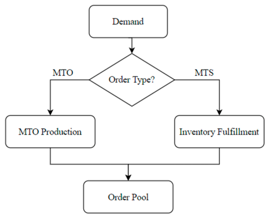
Figure 4.
Confusion matrix for ML models.
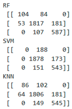
Table 1.
Stages of the Developed Model and the Methods Used.
| Stage | Description | Applied Method |
|---|---|---|
| Order Classification | Orders were classified into priority classes based on their attributes. | Machine learning algorithm |
| Order Evaluation | From the classified orders, those that were feasible under the constraints were identified. | Mathematical model |
Table 2.
Attribute list.
| Attribute | Reference |
|---|---|
| Order Quantity | Wang vd, [17] Arredondo and Martinez [18] Wei and Ma [19] |
| Order Due Date | Wester vd, [6] Wang vd, [17] Kuo and Chen [19] Arredondo and Martinez [18] Kalantari vd, [5] Wei and Ma [19] |
| Order Frequency | Kalantari vd [5] Wei and Ma [19] |
| Production Cost | Ashayeri and Selen [8] Rafiei and Rabbani [9] Abedi and Zhu [1] Kuthambalayan and Bera [21] |
Table 4.
Scenarios used in validation tests.
| Scenario | Number of orders | MTO | MTS | Period | Pj0 | Description | Solution time (s) |
|---|---|---|---|---|---|---|---|
| S1 | 500 | 165 | 335 | 1 | 0 | Model validation | 0,031 |
| S2 | 1000 | 330 | 670 | 1 | 0 | Weekly planning - Small company | 0,062 |
| S3 | 5000 | 1650 | 3350 | 1 | 0 | Weekly planning - Large company | 0,338 |
| S4 | 5000 | 1650 | 3350 | 4 | 0 | Monthly plan | 1,957 |
| S5 | 10000 | 3300 | 6700 | 4 | 0 | Monthly plan - Large company | 2,221 |
| S6 | 10000 | 3300 | 6700 | 12 | >0 | Quarterly planning | 13,987 |
| S7 | 10000 | 3300 | 6700 | 52 | >0 | Annual planning | 1423,194 |
| S8 | 50000 | 16500 | 33500 | 1 | 0 | Large Scale – Single Period | 1,919 |
| S9 | 50000 | 16500 | 33500 | 12 | >0 | Large Scale – Quarterly | 152,754 |
| S10 | 50000 | 16500 | 33500 | 52 | >0 | Annual Period Upper Limit | NA |
| S11 | 100000 | 33000 | 67000 | 1 | 0 | Single Period Limit | 24,608 |
| S12 | 250000 | 82500 | 167500 | 1 | 0 | Single Period Limit | 191,78 |
| S13 | 500000 | 165000 | 335000 | 1 | 0 | Single Period Limit | 760,166 |
| S14 | 1000000 | 330000 | 670000 | 1 | 0 | Single Period Limit | 3829,094 |
| S15 | 1500000 | 495000 | 1005000 | 1 | 0 | Single Period Limit | 9219,865 |
| S16 | 1995000 | 990000 | 1005000 | 1 | 0 | Single Period Upper Limit | NA |
NA: Not available.
Table 5.
Variation of model coefficients.
| Scenario | Description | w(c) | w’(c) | m(c) | MTO acceptance rate | Objective Function Value (Z) |
|---|---|---|---|---|---|---|
| S1 | Base Scenario | 1-2-3 | 1-2-3 | 1-2-3 | 57% | 249946,5 |
| S2 | Narrow Benefit Difference | 1-1,5-2 | 1-1,5-2 | 1-2-3 | 100% | 166644,5 |
| S3 | Wide Benefit Difference | 1-3-9 | 1-3-9 | 1-2-3 | 23% | 749700,5 |
| S4 | Low Penalty | 1-2-3 | 1-2-3 | 1-1,5-2 | 57% | 249946,5 |
| S5 | High Penalty | 1-2-3 | 1-2-3 | 1-3-9 | 57% | 249946,5 |
| S6 | High Benefit and High Penalty | 1-3-9 | 1-3-9 | 1-3-9 | 23% | 749688,5 |
| S7 | MTO Prioritized | 4-5-6 | 1-2-3 | 1-2-3 | 100% | 250044 |
| S8 | MTS Prioritized | 1-2-3 | 1-3-9 | 1-2-3 | 0% | 749664,5 |
| S9 | Increased Penalty Coefficient | 1-2-3 | 1-3-9 | 1-9-27 | 57% | 749610,5 |
| S10 | Proportional Balance | 1-3-9 | 1-3-9 | 1-3-9 | 23% | 749688,5 |
Table 6.
Fleiss’ kappa ccoefficients for the first iteration.
| Subset | Fleiss' kappa coefficient |
|---|---|
| 10% subset | 0,67 |
| 20% subset | 0,74 |
| 30% subset | 0,77 |
Table 7.
Final threshold values.
| Attribute | Threshold 1 | Threshold 2 |
|---|---|---|
| Order quantity | 312 | 4100 |
| Order frequency | 6,36 | 40,86 |
| Due date | 2 | 4 |
Table 8.
Variation of threshold values.
| Variation | Fleiss' kappa coefficient |
|---|---|
| - 5 % | 0,85 |
| - 10% | 0,7 |
| + 5% | 0,87 |
Table 9.
Results of the ML models.
| ML Model | Accuracy Score | Std Dev |
|---|---|---|
| SVM | 0,83 | 0,01 |
| KNN | 0,83 | 0,02 |
| RF | 0,86 | 0,01 |
Table 10.
Classification report.
| ML Model | Class | Precision | Recall | F1-score | Class Percentage % |
|---|---|---|---|---|---|
| RF | 1 | 0,66 | 0,55 | 0,60 | 5,35 |
| RF | 2 | 0,90 | 0,89 | 0,90 | 68,46 |
| RF | 3 | 0,76 | 0,85 | 0,80 | 26,19 |
| SVM | 1 | 0,00 | 0,00 | 0,00 | 0,00 |
| SVM | 2 | 0,85 | 0,92 | 0,88 | 75,59 |
| SVM | 3 | 0,76 | 0,78 | 0,77 | 24,41 |
| KNN | 1 | 0,57 | 0,46 | 0,51 | 5,12 |
| KNN | 2 | 0,88 | 0,88 | 0,88 | 70,13 |
| KNN | 3 | 0,75 | 0,79 | 0,77 | 24,75 |
Table 11.
Model results based on period.
| t | Total Qi | X(i,t) * Total Qi |
Total Fj | Total Yj | Total Production |
Total Requirement |
|---|---|---|---|---|---|---|
| 1 | 41106 | 20348 | 2640216 | 1967349 | 1987697 | 2681322 |
| 2 | 41106 | 41106 | 1536459 | 1536459 | 1577565 | 1577565 |
| 3 | 1944413 | 1430429 | 119863 | 1198639 | 2629068 | 2064276 |
| 4 | 0 | 0 | 1071210 | 1071210 | 1071210 | 1071210 |
| 5 | 0 | 0 | 2524868 | 1858160 | 1858160 | 2524868 |
| 6 | 3186 | 3186 | 1581411 | 1581411 | 1584597 | 1584597 |
| 7 | 1425538 | 1123489 | 1419605 | 1418777 | 2542266 | 2845143 |
| 8 | 621844 | 621844 | 1363119 | 1363119 | 1984963 | 1984963 |
| 9 | 0 | 0 | 2379518 | 1554017 | 1554017 | 2379518 |
| 10 | 0 | 0 | 1549605 | 1549605 | 1549605 | 1549605 |
| 11 | 1452551 | 1230397 | 1656713 | 857690 | 2088087 | 3109264 |
| 12 | 498630 | 458580 | 1205917 | 1013072 | 1471652 | 1704547 |
Disclaimer/Publisher’s Note: The statements, opinions and data contained in all publications are solely those of the individual author(s) and contributor(s) and not of MDPI and/or the editor(s). MDPI and/or the editor(s) disclaim responsibility for any injury to people or property resulting from any ideas, methods, instructions or products referred to in the content. |
© 2026 by the authors. Licensee MDPI, Basel, Switzerland. This article is an open access article distributed under the terms and conditions of the Creative Commons Attribution (CC BY) license (http://creativecommons.org/licenses/by/4.0/).
Copyright: This open access article is published under a Creative Commons CC BY 4.0 license, which permit the free download, distribution, and reuse, provided that the author and preprint are cited in any reuse.


