

Submitted:
22 June 2026
Posted:
24 June 2026
You are already at the latest version
Abstract
The hydroforming performance of trailing arms is governed by the coupled effects of feed parameters, pressure schedules and frictional characteristics. Improper parameter matching readily induces typical forming defects such as wrinkling, cracking and uneven wall thickness. To address this issue, a multi-objective optimization method for hydroforming is proposed in this study. Taking the maximum wall thickness, minimum wall thickness and die-to-workpiece gap of the tubular blank as optimization objectives, and the internal pressure and right-side axial feed velocity as design variables, an integrated numerical simulation framework combining the Archive-based Micro Genetic Algorithm (AMGA) and LS-DYNA is established to analyze the hydroforming process. By adaptively adjusting the key control points of internal pressure and axial feed loading curves, the developed method expands the solution space and realizes the automatic optimization of loading paths. The results reveal that the maximum wall thickness reduction rate of the tubular component is reduced from 20.4% to 14.8%. Meanwhile, the wall thickness uniformity is improved and forming defects are effectively suppressed while the thickening rate remains stable. Moreover, multiple sets of Pareto optimal solutions can be obtained in a single calculation. This work provides new insight into the process optimization for forming similar structural components.
Keywords:
tube hydroforming
; loading path
; torsion beam trailing arm
; AMGA
; optimization
1. Introduction
Torsion beam trailing arms are classified as asymmetric bent tubular components with complex and variable cross-sectional geometries along the axial direction. The two ends of the component feature flat and elliptical cross-sections respectively, without transitional fillets, making such parts well-suited for fabrication via hydroforming [1,2]. The hydroforming process is synergistically governed by multiple process parameters, including internal forming pressure, axial feed displacement, friction coefficient and die corner radius. These parameters exhibit strong coupling and highly nonlinear interaction characteristics. Meanwhile, trade-off relationships commonly exist between different optimization objectives for forming performance [3,4,5]. Conventional single-objective optimization approaches and trial-and-error methods fail to determine the optimal combination of process parameters accurately. Accordingly, it is imperative to develop an efficient multi-parameter collaborative optimization strategy for hydroforming process optimization.
Numerous studies have been conducted worldwide on parameter optimization for tube hydroforming. Wang et al. [6] combined numerical optimization with finite element simulation to determine the optimal loading path for hydroformed T-shaped tubes, and validated the reliability of the proposed method through experimental tests. Aiming at typical defects such as excessive wall thinning and wrinkling during the forming of double-convex tubes. Zhang et al. [7] addressed defects including excessive wall thinning and wrinkling during the forming of double-convex tubes, and clarified the effects of loading path parameters on forming performance via the response surface method. Zheng et al. [8] took automotive instrument panel beams as the research objects. With the wall thickness variation rate as the optimization objective, they adopted the NSGA-II algorithm to optimize key parameters such as internal forming pressure and axial feed displacement, and obtained an optimal forming process scheme. Raut et al. [9] integrated the material constitutive model and ALE numerical technique to characterize material flow behaviors, and completed the hydroforming process optimization using the design of experiments (DOE) and response surface methodology. In addition, multi-objective optimization techniques have been widely applied in various manufacturing fields. Chia et al. [10] systematically summarized the parameter regulation strategies and defect suppression mechanisms for advanced material forming processes. Huang et al. [11] realized the collaborative optimization of crystal preparation processes by integrating prediction models and improved intelligent algorithms. Reddy et al. [12] adopted the MOORA algorithm to achieve efficient parameter optimization for composite manufacturing processes, which provides diverse theoretical references for multi-parameter optimization in plastic forming.
Existing studies mainly rely on finite element simulation, response surface method and NSGA-II to optimize loading paths and process parameters, and employ constitutive models and ALE techniques to analyze material flow. These conventional approaches are restricted by high computational cost and low iteration efficiency, and cannot guarantee both solution accuracy and diversity with small populations. In addition, most conclusions are only applicable to specific components and working conditions, and the understanding of multi-field coupled plastic deformation mechanisms is inadequate [13]. The Archive-based Micro Genetic Algorithm (AMGA) [14] streamlines computation using historical search information and produces high-quality non-dominated solutions efficiently with small populations. It outperforms traditional algorithms in complex multi-objective optimization, yet it has never been applied to tube hydroforming.
In this study, AMGA is coupled with LS-DYNA simulation. Taking wall thickness indicators and die-to-workpiece gap as objectives, and internal pressure and axial feed velocity as design variables, we realize global loading path optimization by regulating key control points of loading curves. The applicability of AMGA in hydroforming is validated to mitigate cracking, wrinkling and other defects, and to provide an efficient approach for complex plastic forming optimization.
2. Models, Equipment and Instruments
2.1. Structural Features of Trailing Arm
The torsion beam trailing arm is arranged along the longitudinal direction of the vehicle body. Its main body is welded to the torsion beam cross member for assembly integration. The front end is hinged to the vehicle body via bushings to achieve longitudinal positioning and serve as a swing pivot, while the rear end is rigidly connected to the wheel bearing housing through a flange structure. This configuration enables effective transmission of driving force, braking force and longitudinal loads during vehicle operation [15,16]. The overall assembly structure is presented in Figure 1(a). As shown in Figure 1(b), the component is a complex hollow part with asymmetric geometry and large curvature. To guarantee forming stability during hydroforming, additional sealing sections, material feeding sections and transition sections are required, as illustrated in Figure 1(c). This trailing arm exhibits dramatic variations in cross-sectional profiles along its axial direction, with flat and elliptical cross-sections at its two ends respectively (Figure 1(d)). The minimum perimeter of the cross section is 209.42 mm, corresponding to an equivalent diameter of 66.67 mm, and the maximum perimeter reaches 293.61 mm with an equivalent diameter of 93.51 mm. The relative difference between the two values is 40.18%. Such a large structural discrepancy from the initial tubular blank leads to considerable difficulties in the forming process (Figure 1(e)).
2.2. Equipment and Die Assembly
The manufacturing of asymmetric bent tubular components consists of multiple procedures including pre-bending, preforming and hydroforming. Multi-stage incremental forming technology acts as a critical technical route for the precision fabrication of complex hollow tubular parts[17,18]. Since the central axis of the torsion beam trailing arm presents an irregular curved profile, the initial straight tubular blank cannot fit the cavity of hydroforming dies directly. For this reason, pre-bending and preforming are adopted as preliminary processes for blank pretreatment, as shown in Figure 2(a). Firstly, the initial straight blank is subjected to axial pre-bending using pipe bending equipment (Figure 2(b)). Afterwards, the pre-bent blank is placed into the preforming die for stamping and shaping (Figure 2(c)). After pretreatment, the axial profile of the tubular blank is basically consistent with the contour of the target hydroforming cavity (Figure 2(d)), which enables reliable assembly and positioning inside the dies. Ultimately, the integral precision forming of the complex trailing arm component is realized using a self-developed 2000-ton hydroforming press (Figure 2(e)).
2.3. Material Property Tests and Material Constitutive Model
The material constitutive model can accurately describe the intrinsic relationship between stress and strain, and acts as a fundamental mechanical basis for guaranteeing the calculation accuracy of finite element numerical simulation in plastic forming [19]. In this work, six groups of standard tensile specimens were machined from the initial tubular blank (Figure 3(a)). Uniaxial tensile tests were then conducted using an electronic universal testing machine, as presented in Figure 3(c), to acquire the engineering stress-strain data of the material (Figure 3(d)). Since engineering stress and strain are calculated based on the original dimensions of specimens, they fail to account for cross-sectional contraction and axial elongation induced by plastic deformation. Accordingly, such data cannot precisely reflect the actual mechanical response during the necking stage [20,21]. For this reason, the engineering stress-strain curve is converted into the true stress-strain curve via theoretical formulas, so as to provide accurate material parameters for subsequent numerical simulation (Figure 3(e)). The specific conversion formulas are given as follows:
Where: : engineering stress (MPa); : engineering strain; : true stress (MPa); : true strain.
To eliminate the distortion of experimental data caused by necking effect, all measured data were truncated at the uniform plastic deformation stage. On this basis, the Swift hardening model was adopted to fit the true stress-strain curves. The fitting results are presented in Figure 3(f), which can provide accurate input parameters for the material constitutive model in subsequent finite element simulations.
Where: : Stress (MPa); : Strain.
3. Hydroforming: Principle and Failure Modes
3.1. Hydroforming Principle
Tube hydroforming is an advanced plastic forming technology evolved from conventional hydraulic bulging [22]. In this process, metal tubes are used as blanks. High-pressure fluid is injected into the sealed tube cavity, and axial thrust is applied at both ends of the tube blank for material feeding. Under the combined action of internal pressure and axial load, the tube blank undergoes plastic deformation and gradually adheres to the die cavity, ultimately forming high-precision hollow structural components [23,24,25]. The forming principle is illustrated in Figure 4.
3.2. Trailing Arm Forming Process
The overall forming process system for torsion beam trailing arms is relatively complex, which consists of multiple critical procedures including blanking, pre-bending, preforming, annealing treatment, hydroforming, laser trimming and punching [26,27] Firstly, high-frequency longitudinal welded steel tubes are cut to specified lengths. The pipe blank is shaped by bending equipment to make its axial profile close to the target configuration. Subsequent preforming and shaping are performed to meet the assembly requirements of hydroforming dies. After annealing, the blank is subjected to hydraulic bulging. Finally, laser cutting is adopted for edge trimming and punching finishing, realizing the integrated manufacturing of finished components.
3.3. Hydroforming Failure Modes
Typical defects such as wrinkling, folding, excessive wall thinning and cracking during the trailing arm forming process are mainly distributed in the hydroforming bulging zone [28]. To clarify the failure mechanism in this forming process, it is essential to analyze the stress and strain characteristics. Assuming that the deformation of tube elements complies with the thin-shell theory, an infinitesimal element is selected arbitrarily within the bulging zone. Its stress state and strain distribution are presented in Figure 5(a) and Figure 5(b), respectively.
According to the volume constancy principle, the strains of the element in three directions satisfy the following equation:
Where: : Circumferential strain of the element; : Axial strain of the element; : Thickness strain of the element.
Stress analysis is conducted on the infinitesimal element in Figure 3(b), and the corresponding governing equations are expressed as:
Where: : Circumferential stress of the element (MPa); : Axial stress of the element (MPa); : Minor radius of curvature of the element (mm); : Major radius of curvature of the element (mm).
The distribution range of the element on the yield locus under plane stress is shown in Figure 5(c). The equivalent stress and equivalent strain under the plane stress condition are formulated as:
Where: : Equivalent stress of the element (MPa); : Equivalent strain of the element.
In tube hydroforming, plastic deformation mainly occurs in the free bulging zone where the tube blank is not in contact with the die cavity. Under the coordinated regulation of forming internal pressure and axial feed, the material in this zone exhibits four typical plastic strain states, which correspond to four forming conditions: no axial feed, insufficient axial compression, balanced axial and circumferential stress, and excessive material feeding [29,30]. The corresponding strain mechanisms are illustrated in Figure 6. During the pressure rising and calibration stages with no axial feed, the tube blank is subjected to biaxial tensile stress. Both axial and circumferential elongation take place simultaneously, leading to remarkable wall thinning, which corresponds to the stress state of Region D in Figure 5. When the axial compressive stress is inadequate to counteract the wall thinning induced by circumferential tension, the material still suffers slight thickness reduction, as represented by Region E in the figure. When a dynamic balance is achieved between axial material feeding and internal pressure, the axial compressive strain effectively compensates for wall thickness loss caused by circumferential tension, thereby realizing circumferential expansion with a constant wall thickness. This condition matches the stress state of Region F. By contrast, excessive axial material feeding results in redundant axial compressive deformation that cannot be converted into circumferential material flow. This phenomenon easily causes material accumulation and wall thickening, and further triggers wrinkling defects, corresponding to the stress state of Region G.
4. Models, Methods and Experiments
4.1. Finite Element Modeling and Methods
4.1.1. Numerical Simulation Model for Hydroforming Analysis
Steel tubes with an outer diameter of 67 mm and a wall thickness of 5.0 mm were used as forming blanks in this work. The initial tube length was set to 958 mm considering product geometry, axial feed stroke, sealing structure and cutting margin. During finite element modelling, the die cavity and end plugs were assigned rigid body properties, and the tube blank was defined as a deformable body. BT shell elements were applied for mesh generation, and SPHC was chosen as the blank material. Constitutive parameters were obtained from the experimental fitting results shown in Figure 3(f), and the constitutive equation is: [31], where stands for true stress and for true strain. Figure 7 shows the developed finite element model.
4.1.2. Selection of Numerical Simulation Algorithms
Compared with the static implicit algorithm, the dynamic explicit algorithm solves the governing dynamic equations step by step via the explicit time integration scheme. It eliminates the need to assemble the global stiffness matrix and can efficiently address strongly nonlinear problems such as complex contact, large plastic deformation, large displacement and large rotation [32,33]. Owing to its excellent adaptability to nonlinear analysis, this algorithm well accommodates the complex deformation characteristics during hydroforming of torsion beam trailing arms, and is therefore adopted for the numerical simulation in this study.
4.1.3. Loading Path Design
The internal pressure loading curve for hydroforming can be divided into four characteristic stages: initial yielding, forming, calibration and pressure holding. Among them, the forming and calibration stages play a decisive role in the forming quality of components. A low-speed pressure rise mode is adopted in the forming stage to ensure stable plastic deformation of the tube blank. In the calibration stage, the pressure rises rapidly, which not only accurately corrects the profile and dimension of components but also shortens the forming cycle and improves processing efficiency. The axial feed displacement curve is dynamically regulated according to forming characteristics. Rapid material feeding is implemented during the forming stage to meet the bulging requirement. Since the blank undergoes negligible deformation in the calibration stage, axial material feeding is basically terminated. Considering the equipment operating conditions, mechanical properties of the material and coupling rules of processes, two internal pressure loading schemes are proposed in this study, namely constant-pressure feeding mode and pressure-rise feeding mode. A comparison of the loading curves is presented in Figure 8.
4.1.4. Evaluate the Effect of Element Size on Forming Results
Mesh element size is a key parameter affecting the accuracy and computational efficiency of finite element simulation. To balance simulation accuracy and the computational efficiency of subsequent multi-objective optimization, a mesh size sensitivity analysis is necessary. Three element sizes of 2 mm, 4 mm and 6 mm were adopted for comparative simulations in this study. The detailed parameters are listed in Table 1, and the wall thickness distribution contours of the component under different mesh schemes are presented in Figure 9.
4.1.5. Experimental Verification
To verify the reliability of the simulated loading paths and the formability of the tube hydroforming process, process experiments were carried out on a self-developed 2000-ton hydroforming apparatus following the conventional loading paths. After integrated processing including tube bending, preforming, annealing and hydroforming, the fabricated specimens exhibited sound forming quality without typical defects such as cracking and wrinkling. Wall thickness comparison was performed at eight characteristic points on five critical cross-sections of the component, as shown in Figure 10. The experimental and numerical results are listed in Table 2. The results reveal that the maximum wall thickness of the component is 5.75 mm with a thickening rate of 15%, and the minimum wall thickness is 4.18 mm with a thinning rate of 16.4%. The wall thickness deviation between experimental measurements and simulation predictions is less than 8% at all detection points, with the maximum deviation of only 7.46%. The two sets of data show good agreement, which effectively validates the accuracy of the established simulation model.
4.2. Optimization Models and Methods
4.2.1. Determination of Design Variables
The trailing arm of the torsion beam features obvious variations in cross-sectional dimensions. Its equivalent diameter at the middle section is 93.8 mm, while the diameter at the end section is only 67 mm. During the pressure rising stage of hydroforming, axial loads are applied to the ends of the tube blank synchronously. This measure overcomes the interfacial frictional resistance and drives material at the ends to flow toward the middle region, which effectively restrains excessive local wall thinning and cracking. Meanwhile, it ensures tight contact between the feeding head and the inner wall of the tube blank, so as to maintain the sealing performance of the forming cavity. It is thus clear that the parameter matching between internal pressure and axial feed loading curves is critical to forming quality. To address the problem of automatic iterative regulation of loading paths in the integrated optimization process, a parametric modeling method based on control points is adopted in this study. The coordinates of key control points on the curves are defined as design variables. The adaptive adjustment of pressure and feed paths is realized by iteratively updating the parameters of control points, which is expressed as:
Where: denotes the control point on the internal pressure loading curve; represents the control point on the axial feed velocity curve, while and are the corresponding time values for the pressure and velocity control points, respectively.
Combined with the structural characteristics of the part and forming process requirements, 12 control points are selected on the pressure curve and 11 on the velocity curve. A total of 23 control points is defined as design variables, and the detailed curves are presented in Figure 11.
4.2.2. Determination of Objective Functions
Compared with straight symmetric tubular parts, the curved-axis trailing arm suffers from severely uneven material flow during hydroforming, which readily induces forming defects such as unilateral wrinkling and fracture, as shown in Figure 12. Optimizing merely for the maximum and minimum wall thickness can suppress wrinkling and cracking, yet fails to guarantee the profile accuracy of the component. Accordingly, the maximum die fitting gap is introduced as the third objective function in this study to quantify forming accuracy and also evaluate the degree of wrinkling. The mathematical expressions of the three objective functions are presented as follows:
Where: ; ; ; : Normal distance from the j-th node on the trailing arm to the die surface; : Thickness of the i-th element after forming; : Coordinate of the j-th node after forming; : Coordinate of the nearest projection point of the j-th node on the die element face after forming; : Unit outward normal vector of the die element face; : Total number of elements; : Total number of nodes.
4.2.3. Selection of Multi-Objective Optimization Method
Common multi-objective optimization algorithms include AMGA, NCGA, MOPSO and NSGA-II. As an improved multi-objective evolutionary algorithm, AMGA screens non-dominated solutions via a small working population and external archive strategy. It features fast convergence, low computational cost and good diversity of Pareto solutions. Therefore, this algorithm is well suited for the time-consuming and highly constrained hydroforming process optimization in this work. The flowchart of AMGA is illustrated in Figure 13.
4.2.4. Multi-Objective Optimization Process
An automated integrated multi-objective optimization system combining LS-DYNA and Python secondary development is established in this study, and the overall iterative workflow is presented in Figure 14. Firstly, LS-DYNA reads the K file containing design variables, material parameters, die models and preforming results, conducts the hydroforming simulation, and outputs the dynain result file. Simulation data are subsequently extracted via Python scripts to calculate the maximum wall thickness, minimum wall thickness of the component and the maximum fitting gap between the component and die, followed by data export. Afterwards, the AMGA solver imports the target parameters to compute the population fitness, screen non-dominated solutions and update the external archive. Redundant individuals are eliminated based on the crowding distance mechanism to maintain the diversity of solution sets. The design variables are continuously updated throughout iterations, and the simulation loop repeats until the maximum iteration number is reached. Finally, the optimal Pareto solution set is obtained and output.
5. Results Evaluation
5.1. Simulation Results
The key parameters of the Archive Micro-Genetic Algorithm (AMGA) were configured in this study. Both the initial population size and evolutionary population size were set to 160. The upper limits of the global archive and non-dominated solution set were defined as 500 and 200, respectively. The crossover probability and mutation probability were specified as 0.9 and 0.5, with corresponding distribution indices of 10 and 20. The maximum number of simulation evaluations was limited to 1600. The calculation results are presented in Figure 15. Each data point in the figure represents a feasible solution set. A smaller maximum wall thickness , smaller maximum fitting clearance and larger minimum wall thickness can substantially improve the forming quality and weight reduction performance of the tubular component. Accordingly, the solution sets located near the inner corner of Figure 15 are identified as the optimal solutions for this multi-objective optimization problem.
Figure 16 presents the simulation results, where the horizontal axis denotes the iteration number, and the vertical axes represent the maximum wall thickness , minimum wall thickness , and normal clearance between the tube blank and die.The results show that ranges from 5.37 mm to 7.68 mm, with the corresponding thickening rates of 7.4% and 53.6% respectively. Severe wrinkling occurs when the thickening rate reaches 53.6%. The values of vary between 0.83 mm and 4.33 mm, leading to thinning rates of 83.4% and 13.4%. An extremely high thinning rate of 83.4% causes excessive local thinning and even cracking of the tube blank. In addition, is measured from 0.52 mm to 8.56 mm. A clearance of 0.52 mm indicates an excellent contact condition between the trailing arm and die, and full fitting can be achieved by moderately increasing the forming pressure. By contrast, the maximum clearance of 8.56 mm induces prominent wrinkling and results in forming failure. Overall, the loading paths of internal pressure and axial feed are the dominant factors governing the forming quality and forming reliability of the tubular component.
Figure 17 shows the three-objective Pareto optimal front obtained via the AMGA together with its two-dimensional projection. The optimal solution set converges uniformly onto a continuous and irregular spatial surface, which exhibits good integrity without obvious vacancies or inferior scattered solutions. This verifies the excellent convergence and global optimization capability of the proposed algorithm. The analysis reveals that both and increase with the rise of . Nevertheless, no monotonic correlation exists between and , and presents remarkable uncertainty within a certain range. In addition, even when reaches its optimal value, cracking may still occur if the minimum wall thickness is less than 3.0 mm. In contrast, an excessively large will trigger severe wrinkling and eventually lead to forming failure. Therefore, it is essential to accurately evaluate the influence of on the matching performance between process parameters and equipment machining conditions.
To further verify the technical feasibility of the optimal solutions, three Pareto optimal solutions with of 0.73 mm, 1.09 mm and 2.0 mm were selected for evaluation, and the corresponding results are presented in Figure 18. The analysis indicates that the forming pressure required to eliminate die surface clearance rises remarkably with the increase of . As increases from 0.73 mm to 1.09 mm, the maximum required forming pressure grows from 200 MPa to 400 MPa, representing a 100% increment. Moreover, the relatively large clearance cannot be fully eliminated even under a forming pressure of 400 MPa.This reveals that several theoretical Pareto optimal solutions fail to satisfy practical process constraints and carry risks of engineering failure. Meanwhile, the selection mechanism of the AMGA may also exclude some technically feasible solutions. Thus, further screening and verification are urgently required.
Given the mismatch between the aforementioned theoretical optimal solutions and practical manufacturing processes, a secondary screening was performed on the 1698 solution sets output by the AMGA, including 2 invalid solutions and all Pareto optimal solutions. Combined with the plastic forming characteristics of materials, equipment operating limits, practical production experience and simulation rules, the constraint thresholds for forming evaluation were defined as follows: the upper limit of : was 6.0 mm, the upper limit of was 1.0 mm, and the lower limit of was 3.8 mm. The screening results are illustrated in Figure 19, where all scattered points represent process-feasible solutions. Comparative analysis shows that the number of feasible solutions within the Pareto optimal set is obviously lower than that of all practical feasible solutions, which is attributed to the inherent screening mechanism of the AMGA. This algorithm only retains optimal solutions that satisfy the non-dominated relationship, uniform distribution and hard constraints, and eliminates redundant solutions via multiple procedures such as archive screening, crowding distance trimming, evolutionary selection and constraint judgment. To maintain the diversity of solution sets and avoid aggregation on the Pareto front, densely distributed non-dominated feasible solutions are trimmed, while dominated feasible solutions with low crowding degree are directly discarded. In conclusion, the loss of partial feasible solutions is an inevitable outcome of the multi-stage screening and optimization of the algorithm, which is a normal convergence characteristic of multi-objective optimization.
5.2. Re-Optimization of Results
The aforementioned unconstrained simulation optimization was performed to expand the solution space and obtain abundant Pareto optimal solutions, so as to provide sufficient alternatives for forming process planning and process parameter matching. Nevertheless, the solution set acquired under this mode features a wide coverage and a large quantity, containing numerous invalid solutions that violate practical engineering constraints.
Accordingly, constraint conditions were imposed on the objective functions to screen qualified optimal solutions, ensuring that the optimized results can be directly adopted for practical process design. With all other parameters kept unchanged, the upper bounds of and were set to 6.5 mm and 1.0 mm, respectively, while the lower bound of was moderately relaxed to 3.5 mm. The results of constrained optimization are presented in Figure 20. It is observed that the optimized solution set converges uniformly to a complete and continuous irregular spatial surface, and all optimal solutions comply with process specifications. Compared with unconstrained optimization, the solution set of constrained optimization is confined within the feasible region, with its scale and coverage remarkably reduced. Only non-dominated solutions satisfying process requirements are retained. In addition, when the upper bound of was set to 0.73 mm, no Pareto optimal solutions that meet the constraint requirements were generated after optimization.
5.3. Correlation Analysis
Table 3 lists the correlation coefficients between each design variable and optimization objective under unconstrained optimization conditions. As shown in the table, variables P6~P8 and V8~V10 are positively correlated with , while the remaining pressure and velocity variables exhibit no significant correlation with . P6 presents a negative correlation with , and V4–V6 show a positive correlation with . Most design variables exert weak or negligible effects on . In addition, individual pressure or velocity variables are weakly correlated or uncorrelated with . Further analysis on the correlation mechanism indicates that internal pressure acts as the core factor regulating the wall thickness uniformity of the tube blank. A higher internal pressure increases the interfacial friction resistance, restricts the material flow from the end region to the forming zone, and consequently leads to wall thickening at the ends and excessive thinning in the middle section. This finding is consistent with theoretical deductions and practical engineering experience. The effect of feeding velocity on wall thickness distribution varies at different forming stages. A high feeding velocity during the mid-stage of forming aggravates wall thinning and deteriorates thickness uniformity, whereas reducing the feeding velocity in the late forming stage can effectively mitigate thickening and thinning defects. Meanwhile, is predominantly governed by die cavity precision, initial blank dimensions, and the matching curve of pressure and axial feed (i.e., loading path), rather than a single process parameter. Accordingly, improving the die-fitting accuracy of tubular components requires priority optimization of the coordinated loading path, instead of simply adjusting internal pressure or feed velocity. The correlation distribution between partial variables and objective parameters is illustrated in Figure 21.
5.4. Discussion on Schemes
To systematically verify the engineering effectiveness of the optimized results, three sets of hydroforming loading path schemes were designed in this study, and the detailed parameters are presented in Figure 22. Scheme A adopts a constant internal pressure combined with bidirectional axial feeding. Scheme B applies a loading mode where the internal pressure increases synchronously with axial feeding. Scheme C corresponds to the optimal loading strategy obtained via the present optimization. The left-side feeding curves remain identical across all three schemes, and the total simulation duration is set to 25 ms. Notably, the left-side feeding displacement of Scheme C is only 15.8 mm. This arrangement is designed to counteract interfacial friction resistance and achieve end sealing of the tube blank.
Figure 23 shows the wall thickness contours of the trailing arm under three loading plans. All three plans enable sound forming of the tubular component. The minimum wall thicknesses of Plan A, Plan B and Plan C are 3.98 mm, 4.06 mm and 4.26 mm, with wall thinning rates of 20.4%, 18.8% and 14.8% correspondingly. Their maximum wall thicknesses and thickening rates are 5.57 mm (11.4%), 5.40 mm (8%) and 5.62 mm (12.4%). Compared with the control plans, the optimized Plan C obviously alleviates wall thinning.
As can be seen from Figure 24, the maximum feeding displacement of Plan A and Plan B is 57 mm. For Plan C, this value rises by 11.3 mm to 68.3 mm, which greatly improves the forming quality.
6. Conclusions
This study establishes a multi-objective optimization model for hydroforming of automotive trailing arms. The optimization objectives include the maximum wall thickness, minimum wall thickness of the tube blank, and the clearance between the trailing arm and die, while the internal pressure and axial feeding velocity on the right side are defined as design variables. The loading path for hydroforming is optimized using the AMGA. The main conclusions are summarized as follows:
(1) Hydroforming of complex structural components is characterized by high-dimensional parameter coupling and mutual restriction among multiple objectives. The AMGA is adopted for simulation optimization in this work, which effectively addresses the drawbacks of traditional algorithms, such as slow convergence, insufficient solution diversity and susceptibility to local optima. This study fills the research gap regarding the application of the AMGA in the hydroforming field, and provides a valuable reference for process optimization of similar components.
(2) Compared with conventional empirically designed loading schemes, the optimized loading path proposed herein substantially improves the forming quality of components. The maximum wall thinning rate of the tubular part is reduced from 20.4% to 14.8%, while the wall thickening performance is well maintained. Multiple sets of Pareto optimal solutions can be obtained in a single iteration, offering diverse alternatives for hydroforming process planning and parameter matching.
(3) The hydroforming process of tubular parts is well suited to the collaborative loading mode with variable internal pressure and variable feeding velocity. Correlation analysis reveals that the axial feeding velocity acts as a core parameter governing the forming quality. A segmented dynamic feeding strategy, namely low feeding velocity at the initial and final forming stages to suppress wrinkling and increased velocity in the middle stage, can effectively avoid typical forming defects such as excessive thinning and cracking.
(4) Physical experiments are carried out on a self-developed 2000-ton hydroforming apparatus to verify the engineering feasibility of the proposed optimization method. The experimental results show good agreement with the simulation predictions, with a maximum error of only 7.46%. The optimized loading path effectively alleviates the excessive wall thinning at the middle section and material accumulation at the ends induced by traditional processes. The proposed method is applicable to the forming of tubular parts with complex cross-sections, and provides reliable theoretical and technical support for intelligent manufacturing of profiled tubular components.
Author Contributions
Zaixiang Zheng: Conceptualization, Methodology, Software, Validation, Resources, Funding acquisition, Writing - original draft. Hui Tan: Validation, Formal analysis, Visualization, Writing - review & editing. Gang Wu: Validation, Data curation. Feng Wang: Investigation, Formal analysis. Siyuan Tang: Investigation, Software, Data curation. Yujie Chen: Investigation, Visualization, Formal analysis. Yang Zhao: Software, Investigation, Validation. Hantao Yu: Data curation, Investigation, Visualization. Zhengjian Pan: Project administration, Data curation.
Data Availability Statement
The authors confirm that the supporting data for this study’s conclusion are included in the manuscript. Raw simulation and experimental data are available from the corresponding author upon reasonable request.
Acknowledgments
This work is supported by the National Natural Science Foundation of China (Grant No. 52306167) and Jiangsu Naite Internal High Pressure Forming Technology Co., Ltd. (Grant No. 5012/204034814).
Conflicts of Interest
No potential conflict of interest was reported by the author(s).
References
- Huang, Y.; Li, J.; Yang, J.C.; et al. Simulation Analysis of Torsion Beam Hydroforming Based on the Fluid-Solid Coupling Method. Chin. J. Mech. Eng. 2023, 36, 3. [Google Scholar] [CrossRef]
- Li, J.; Li, Y.J.; Liang, P.; et al. Research on the hydroforming law of variable cross-section shaped tubular automobile longitudinal arm. Arch. Civ. Mech. Eng. 2024, 25, 3. [Google Scholar] [CrossRef]
- Zhang, X.L.; Xiao, J.; Xie, X.D.; et al. Bending-hydraulic forming stainless steel thin-walled tube fittings wall thickness distribution law research. Int. J. Lightweight Mater. Manuf. 2025, 8, 402–14. [Google Scholar] [CrossRef]
- Cusanno. Optimizing sheet hydroforming process parameters with a focus on sustainability; 2025; pp. 2494–502. [Google Scholar] [CrossRef]
- Modanloo, V.; Akhoundi, B.; Khatir, F.A.; et al. Investigation of the effect of process parameters in sheet hydroforming process. Int. J. Interact. Des. Manuf. 2023, 17, 3189–98. [Google Scholar] [CrossRef]
- Wang, L.; Xu, X.F.; Fan, Y.B.; et al. Loading path design of thin-walled aluminum alloy T-shaped tube hydroforming process based on the control of limit pressure. Int. J. Adv. Manuf. Technol. 2020, 108, 3119–31. [Google Scholar] [CrossRef]
- Zhang; Liu, W.; Huang, L.R.; et al. Process analysis of biconvex tube hydroforming based on loading path optimization by response surface method. Int. J. Adv. Manuf. Technol. 2021, 112, 2609–22. [Google Scholar] [CrossRef]
- Zheng, Z.X.; Yao, Z.H.; Pan, Z.J. Optimization of loading path for internal high-pressure forming of instrument panel tube beam based on NSGA-II. J. Eng. Appl. Sci. 2025, 72, 77. [Google Scholar] [CrossRef]
- Raut, S.V.; Ramesh, A.; Arun, A.; et al. Finite element analysis and optimization of tube hydroforming process. Mater. Today Proc. 2021, 46, 5008–16. [Google Scholar] [CrossRef]
- Chia, H.Y.; Wu, J.Z.; Wang, X.; et al. Process parameter optimization of metal additive manufacturing: a review and outlook. J. Mater. Inf. 2022, 2, 16. [Google Scholar] [CrossRef]
- Huang, W.C.; Li, R.Z.; Wu, R. Modeling of Quality Factor and Process Parameter Optimization in Czochralski Silicon Single Crystal Growth. 2025 44th Chinese Control Conference (CCC), Chongqing, China, 2025; IEEE; pp. 6857–62. [Google Scholar] [CrossRef]
- Reddy, P.L.; Kumar, A.S.; Mahesh, P.; et al. Drilling of Al-MMC and its process parameters optimization; Medan, Indonesia, 2022; p. 040013. [Google Scholar] [CrossRef]
- Chen, Z.H.; Liu, S.X.; Chen, Z.; et al. A Multi-Objective Salp Swarm Algorithm Based on Strength Pareto. 2025 44th Chinese Control Conference (CCC), Chongqing, China, 2025; IEEE; pp. 2346–51. [Google Scholar] [CrossRef]
- Tiwari, S.; Koch, P.; Fadel, G.; et al. Amga. In Proceedings of the 10th annual conference on Genetic and evolutionary computation; 2008; pp. 729–36. [Google Scholar] [CrossRef]
- Chung, K.; Lee, Y.; Lee, J. The Analysis of Stiffness and Driving Stability in Cross-Member Reinforcements Based on the Curvature of a Small SUV Rear Torsion Beam Suspension System. Appl. Sci. 2023, 13, 12067. [Google Scholar] [CrossRef]
- Gao, J.; Qi, X. Position design of the trailing arm bushing on torsion beam suspension accounting for vehicle transient handling performance and uncertainties. Adv. Mech. Eng. 2023, 15, 16878132231193348. [Google Scholar] [CrossRef]
- Zhu, H.; Cheng, G.; Jung, D. Toolpath Planning and Generation for Multi-Stage Incremental Forming Based on Stretching Angle. Materials 2021, 14, 4818. [Google Scholar] [CrossRef] [PubMed]
- Palwai, S.R.; Bharti, S.; Tiwari, A.K.; et al. Mathematical approach to design preform for multi stage robot assisted incremental forming. Int. J. Mater. Form. 2025, 18, 62. [Google Scholar] [CrossRef]
- Zhang, X.; Gao, F.; Li, Y.; et al. An Exponential Drucker-Prager Constitutive Model of Polyurethane Adhesive for Finite Element Model Simulation. J. Appl. Polym. Sci. 2025, 142, e56514. [Google Scholar] [CrossRef]
- Kim, J.; Gu, G.H.; Kwon, J.; et al. A Novel Framework for Evaluating the Intrinsic Mechanical Properties of Sheet Metals Using Two-dimensional Digital Image Correlation. Met. Mater. Int. 2025, 31, 2837–44. [Google Scholar] [CrossRef]
- Mirone, G.; Barbagallo, R.; Bua, G.; et al. A Simple Procedure for the Post-Necking Stress-Strain Curves of Anisotropic Sheet Metals. Metals 2023, 13, 1156. [Google Scholar] [CrossRef]
- Sadłowska, H.; Morawiński, Ł.; Jasiński, C. Strain Measurements in Free Tube Hydroforming Process. Arch. Metall. Mater. 2020, 257–63. [Google Scholar] [CrossRef]
- Marlapalle, B.G.; Hingole, R.S. Predictions of formability parameters in tube hydroforming process. SN Appl. Sci. 2021, 3, 606. [Google Scholar] [CrossRef]
- Yasui, H.; Miyagawa, T.; Yoshihara, S.; et al. Influence of Internal Pressure and Axial Compressive Displacement on the Formability of Small-Diameter ZM21 Magnesium Alloy Tubes in Warm Tube Hydroforming. Metals 2020, 10, 674. [Google Scholar] [CrossRef]
- Rudraksha, S.P.; Gawande, S.H. Effect of Process Parameters on Coefficient of Friction in Tube Hydroforming. J. Bio Tribo Corros. 2021, 7, 9. [Google Scholar] [CrossRef]
- Zhang, Z.; Xu, F.; Sun, X. Optimization of process parameters during hydroforming of tank bottom using NSGA-III algorithm. Int. J. Adv. Manuf. Technol. 2022, 119, 4043–55. [Google Scholar] [CrossRef]
- Zhang, Z.; Kang, Y.; Furushima, T.; et al. Deformation behaviour of metal micro tube during hydroforming process. Procedia Manuf. 2020, 50, 328–31. [Google Scholar] [CrossRef]
- Zhu, H.; Xu, Y.; Khina, B.B.; et al. Impact hydroforming characteristics for a half-tube part with curvature. Chin. J. Aeronaut. 2026, 39, 103455. [Google Scholar] [CrossRef]
- Yan; Meng, B.; Wan, M. A 3D defect-driven analytical framework linking geometric evolution to failure limits in ring hydroforming. Int. J. Mach. Tools Manuf. 2026, 219, 104412. [Google Scholar] [CrossRef]
- Gallifa-Terricabras; Swieszek, J.S.; Smakulska, D.; et al. Forming limit diagram of annealed copper OFE thick sheets for optimized hydroforming of superconducting RF cavities. Mater. Des. 2024, 244, 113191. [Google Scholar] [CrossRef]
- Lei, X.Z.; Fu, W.X.; Liao, Y. Multi-Segment Linear Function Approximation of the Nonlinear Shear Strength Envelope. Strength Mater. 2016, 48, 460–468. [Google Scholar] [CrossRef]
- An explicit time integration algorithm for linear and non-linear finite element analyses of dynamic and wave problems. Eng. Comput. 2019, 36, 161–77. [CrossRef]
- Fu, B.; Lavery Ilunga, S.; Chen, J. Two families of dual-explicit model-based integration algorithms with controllable numerical damping for structural dynamic problems. Mech. Syst. Signal Process. 2024, 218, 111576. [Google Scholar] [CrossRef]
Figure 1.
Trailing arm structural features: (a) Torsion beam assembly, (b)Trailing Arm, (c) Hydroforming die cavity, (d) Cross-sectional shapes, (e) Outer perimeter of cross section.
Figure 1.
Trailing arm structural features: (a) Torsion beam assembly, (b)Trailing Arm, (c) Hydroforming die cavity, (d) Cross-sectional shapes, (e) Outer perimeter of cross section.
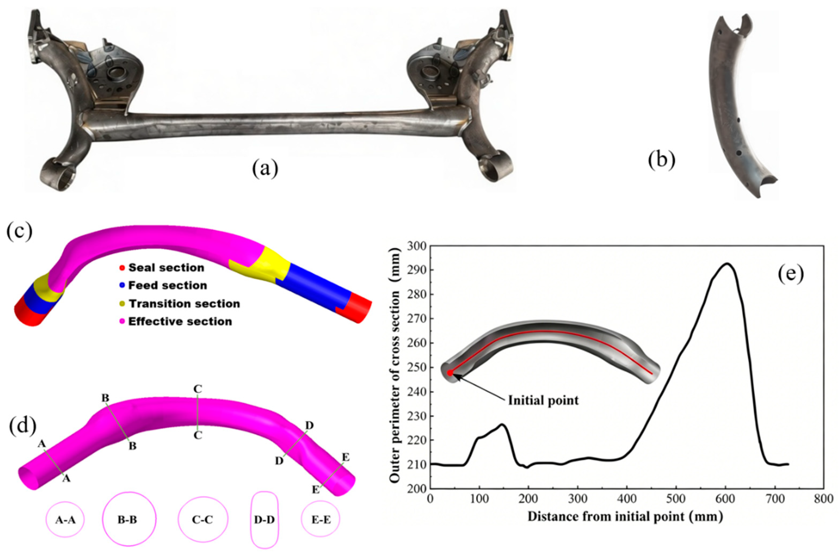
Figure 2.
Equipment and die assembly: (a) Forming process of trailing arm, (b) Initial tubular blank, (c) Preforming die, (d) Hydroforming die, (e) 2000-ton hydraulic forming press.
Figure 2.
Equipment and die assembly: (a) Forming process of trailing arm, (b) Initial tubular blank, (c) Preforming die, (d) Hydroforming die, (e) 2000-ton hydraulic forming press.
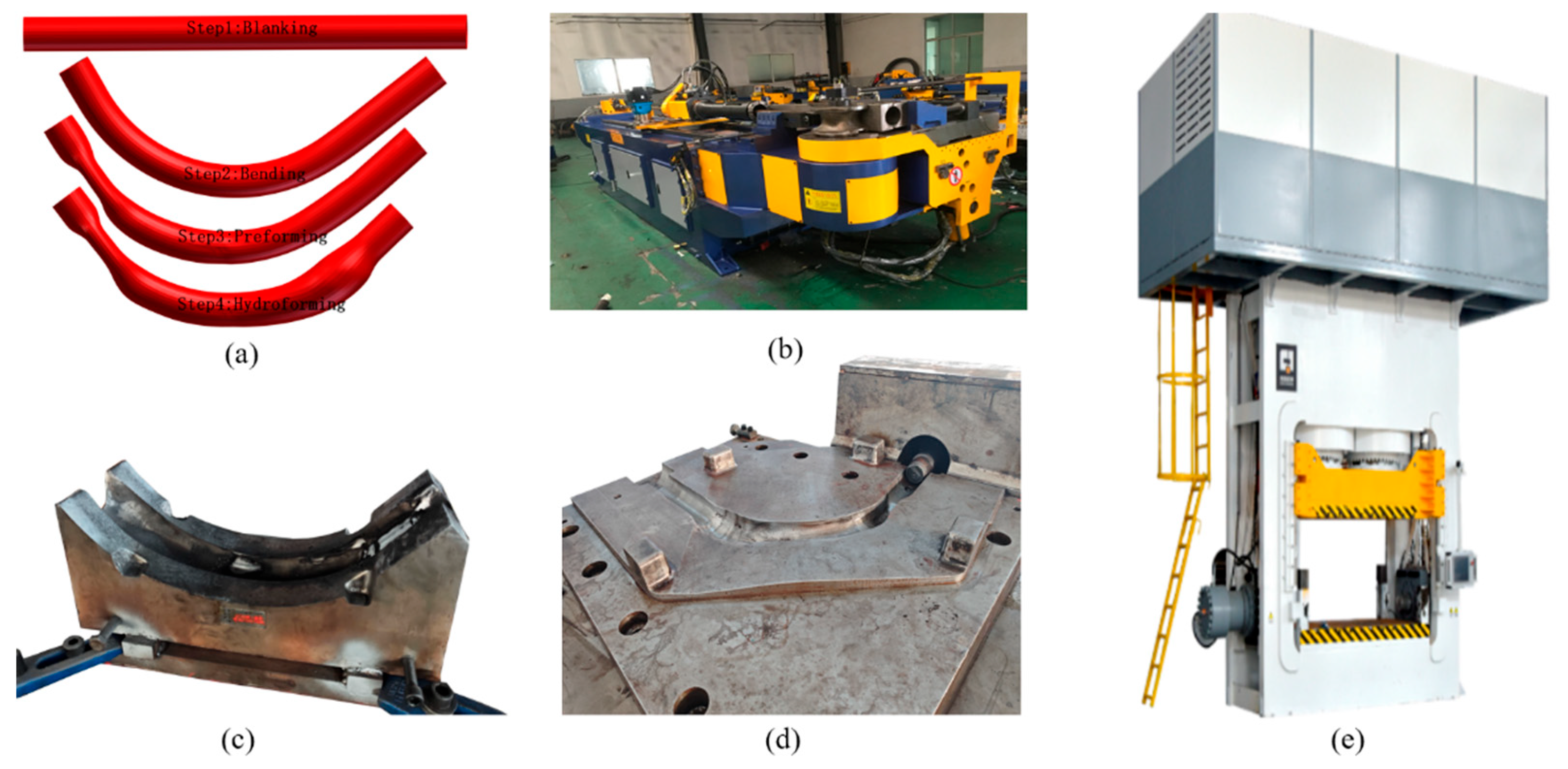
Figure 3.
Material testing and data processing: (a) Tube, (b) Standard specimen, (c) Tested Specimens, (d) Engineering stress-strain curve, (e) True stress-strain curve, (f) Fitted true stress-strain curve.
Figure 3.
Material testing and data processing: (a) Tube, (b) Standard specimen, (c) Tested Specimens, (d) Engineering stress-strain curve, (e) True stress-strain curve, (f) Fitted true stress-strain curve.
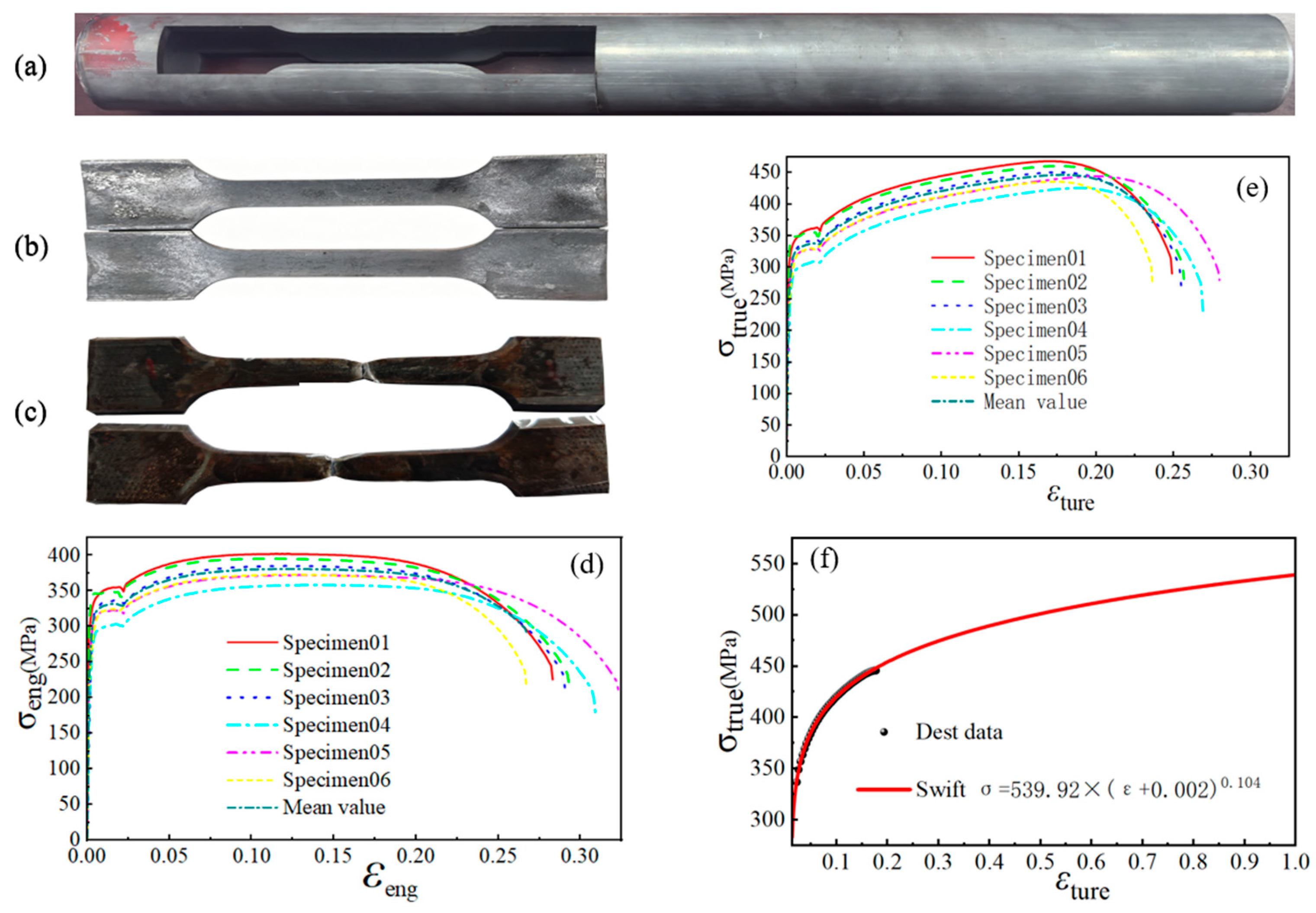
Figure 4.
Schematic of tube hydroforming principle.
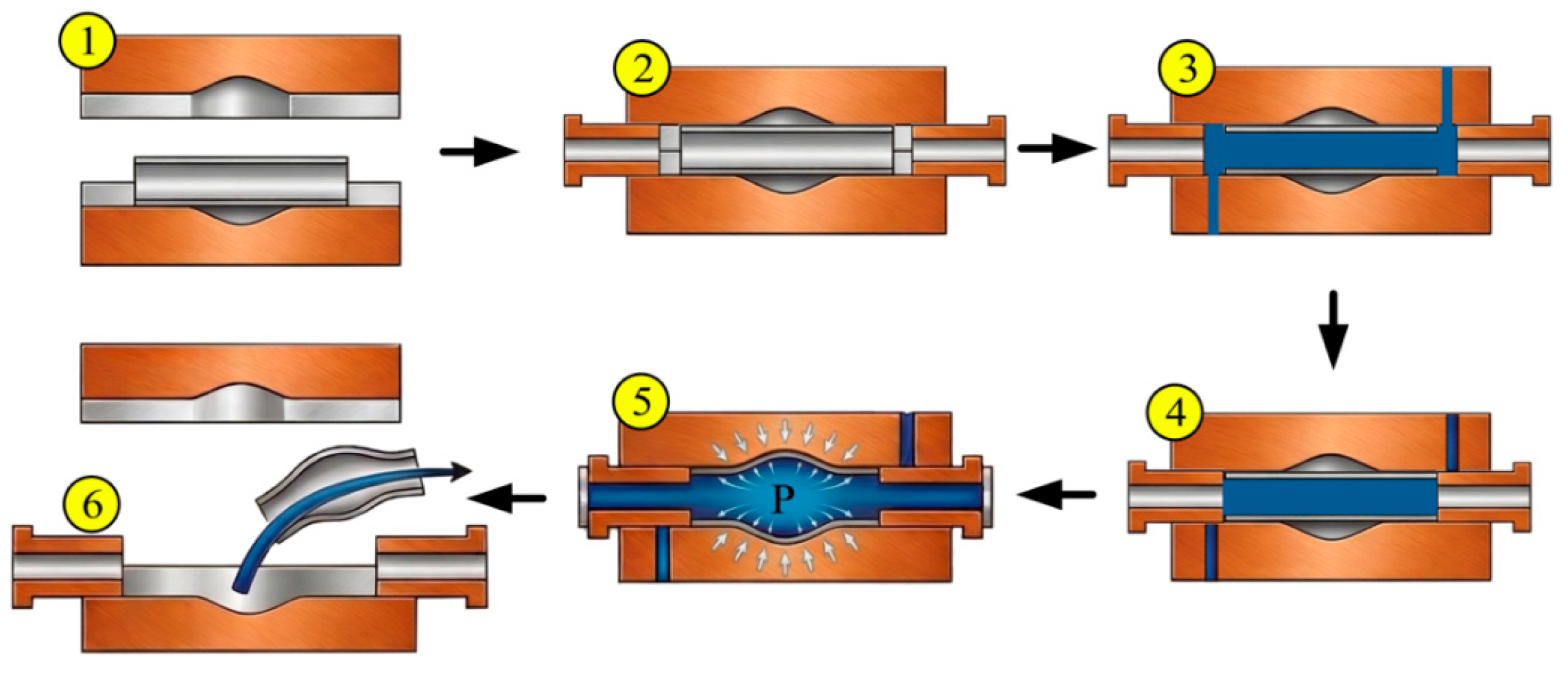
Figure 5.
Stress and strain state of micro-element: (a) Strain condition, (b) Stress condition, (c) Distribution range of micro-element on the yield locus under plane stress.
Figure 5.
Stress and strain state of micro-element: (a) Strain condition, (b) Stress condition, (c) Distribution range of micro-element on the yield locus under plane stress.
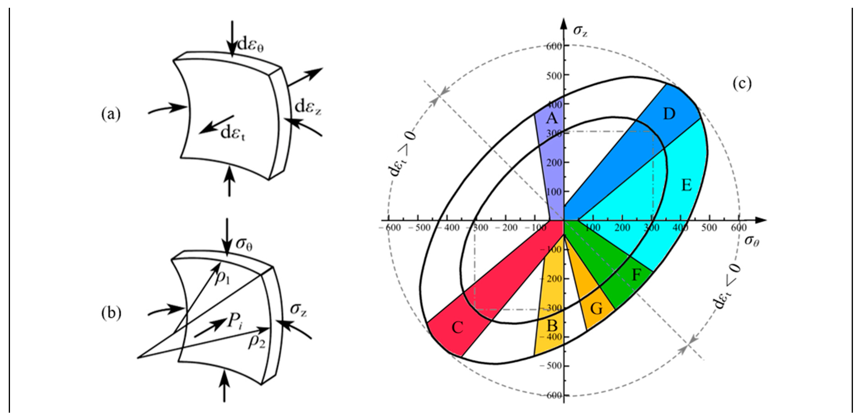
Figure 6.
Stress and plastic deformation state of micro-element during hydroforming.
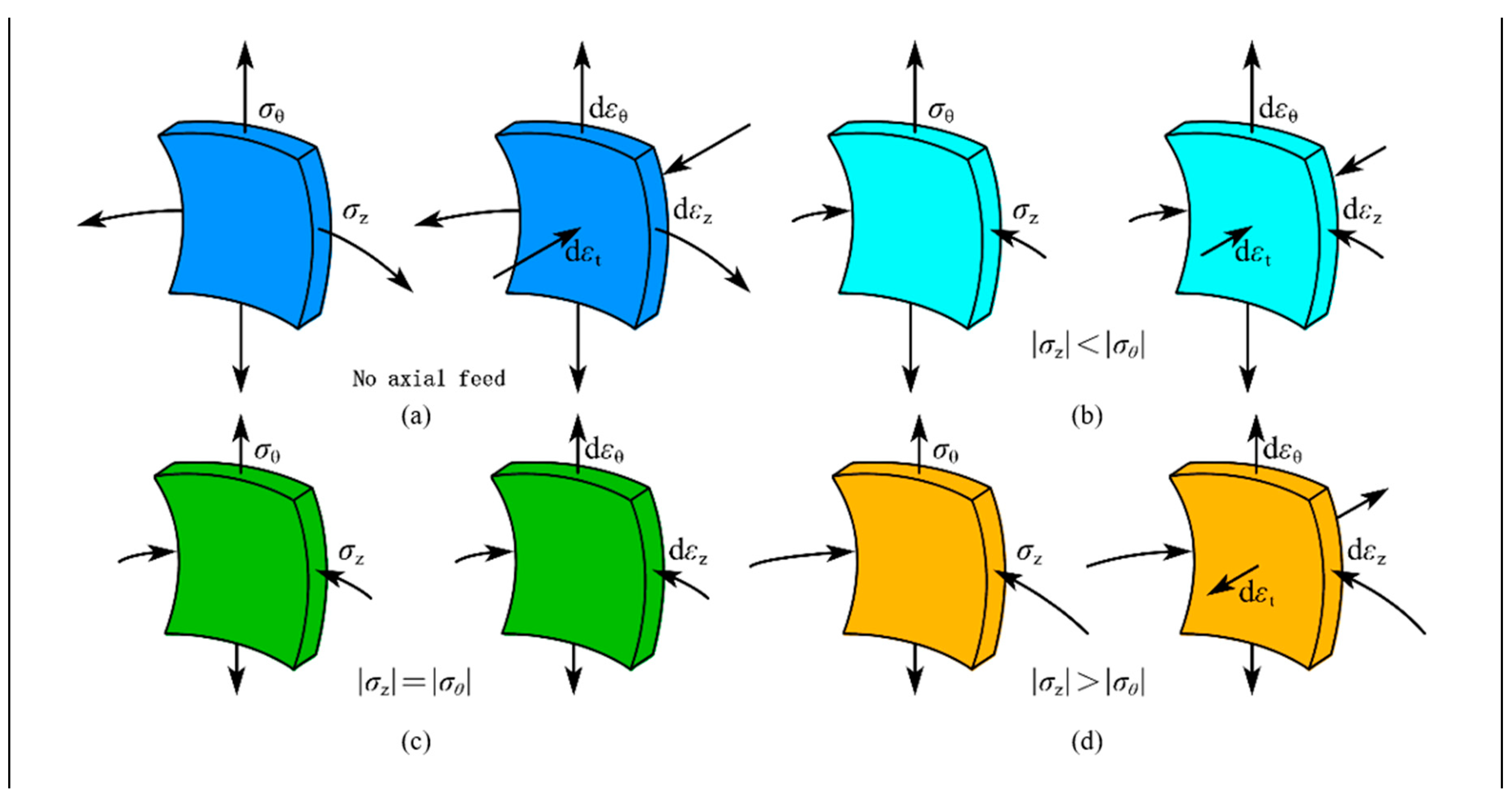
Figure 7.
Finite element model: 1. Left plug, 2. Lower die, 3. Upper die, 4. Tube blank, 5 Right plug.
Figure 7.
Finite element model: 1. Left plug, 2. Lower die, 3. Upper die, 4. Tube blank, 5 Right plug.
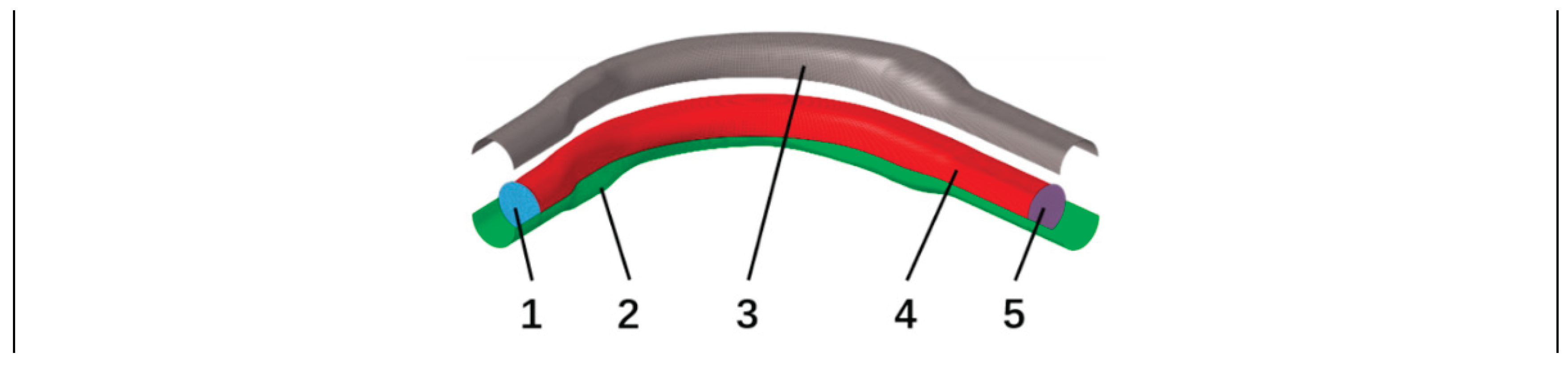
Figure 8.
Axial feed and internal pressure loading curves.
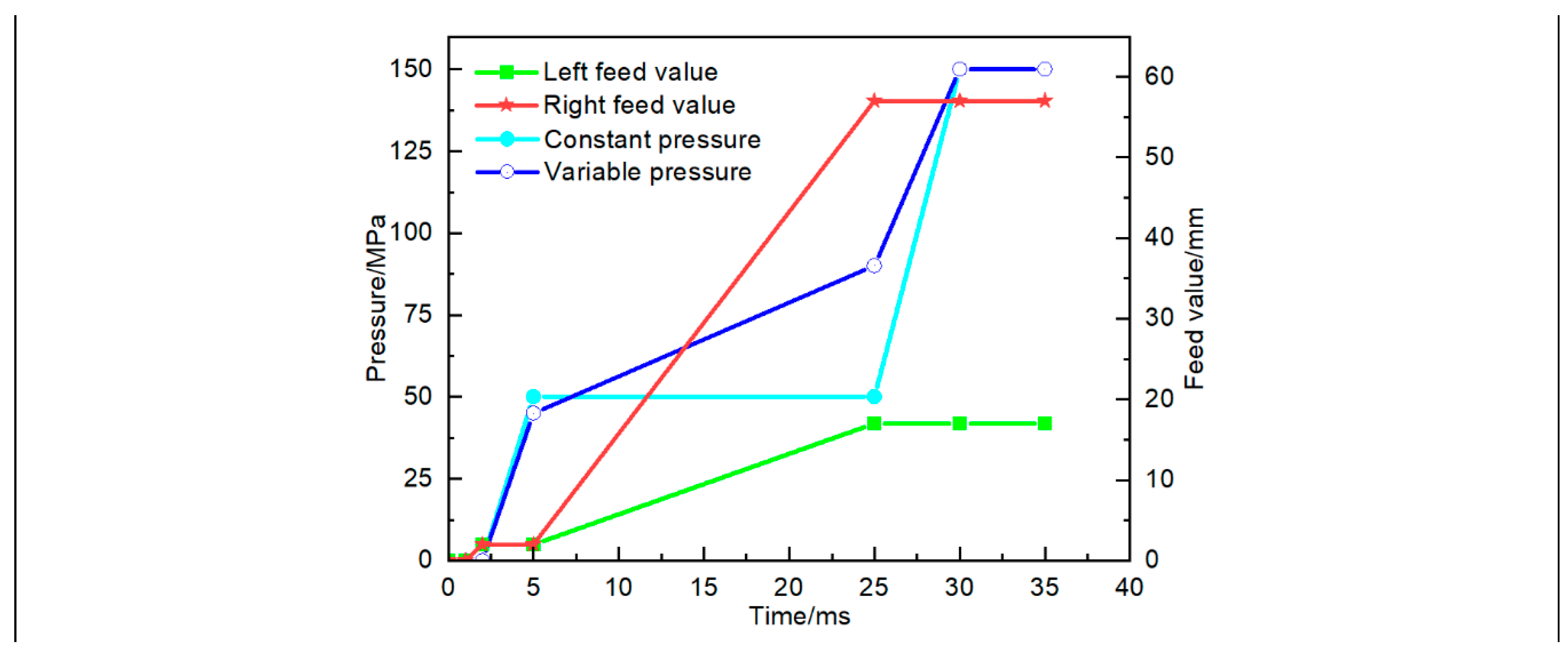
Figure 9.
Wall thickness contours under different mesh sizes: (a)2mm, (b)4mm, (c)6mm.
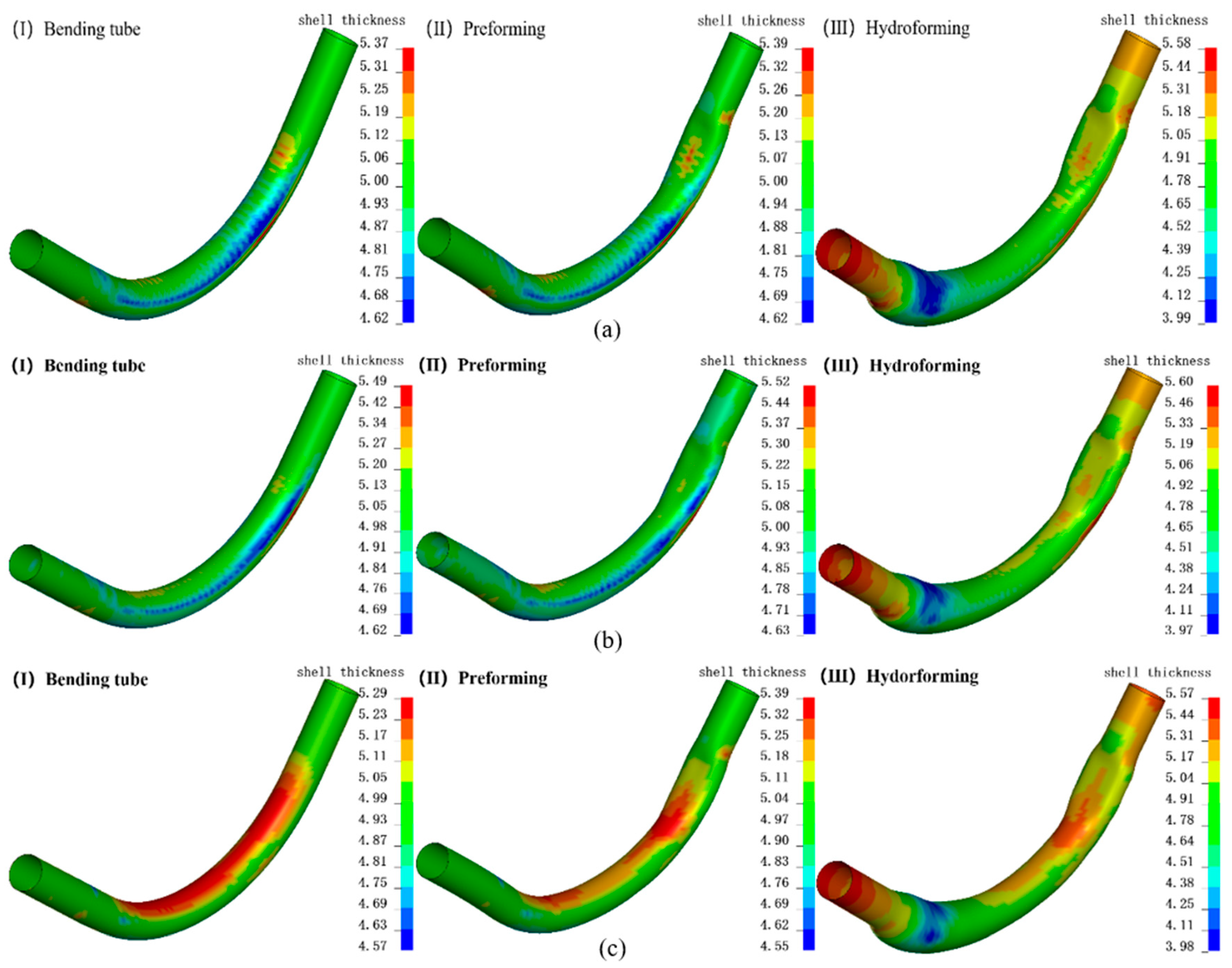
Figure 10.
Thickness distribution of different section characteristics.
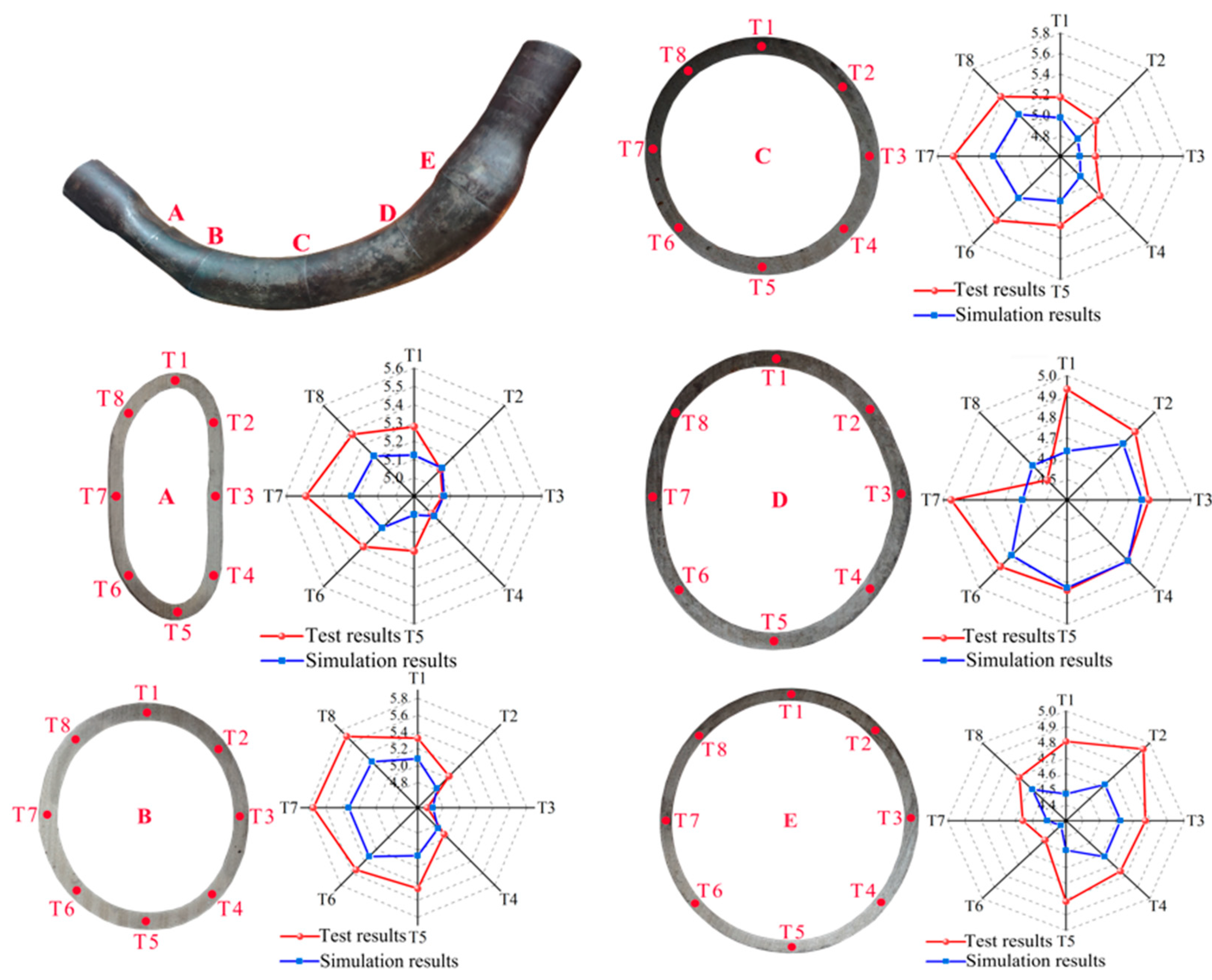
Figure 11.
Internal pressure and axial feed velocity design variables:(a) Internal pressure control points and their boundaries, (b) feed velocity control points and their boundaries.
Figure 11.
Internal pressure and axial feed velocity design variables:(a) Internal pressure control points and their boundaries, (b) feed velocity control points and their boundaries.
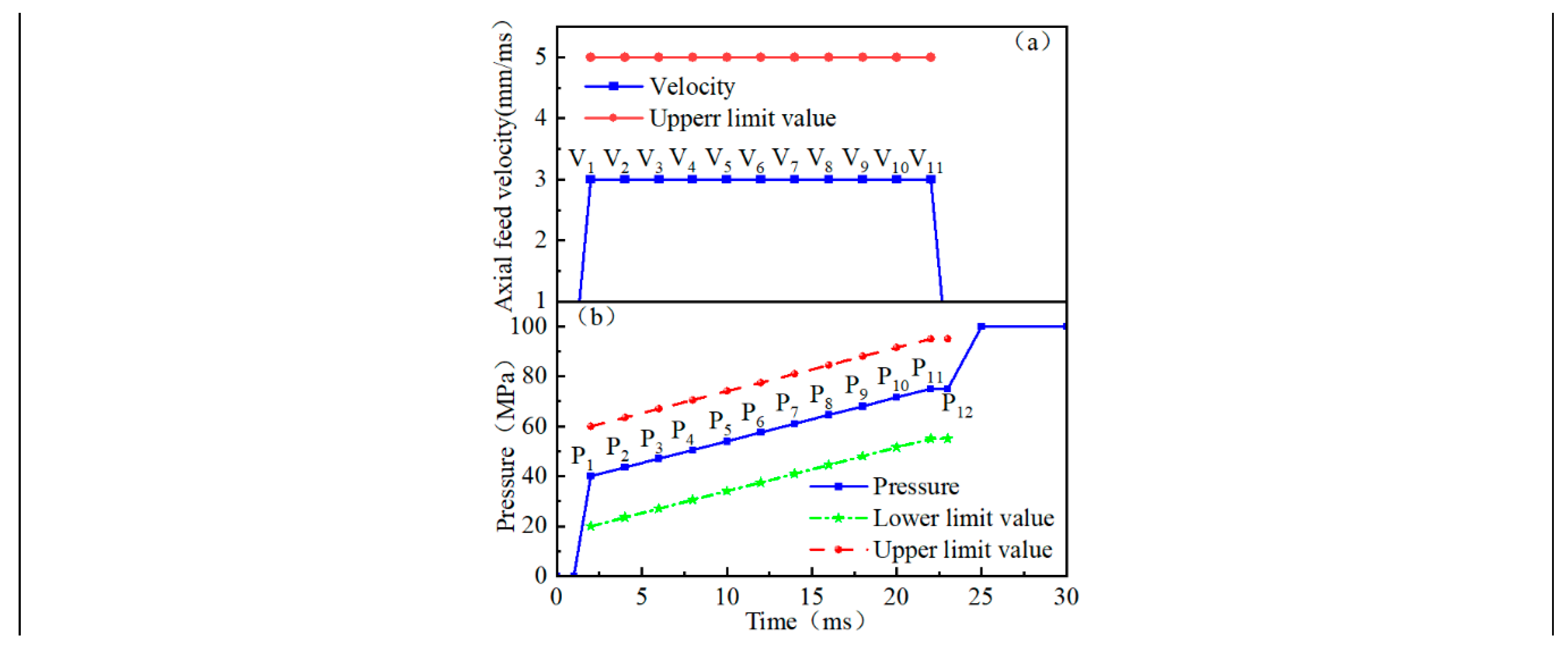
Figure 12.
Wrinkling defects in tube hydroforming.
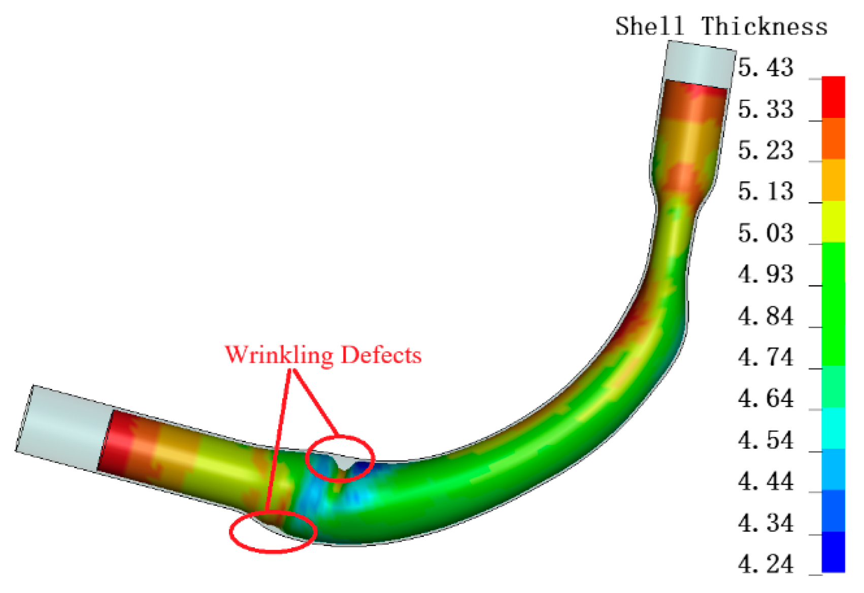
Figure 13.
Flowchart of the AMGA algorithm.
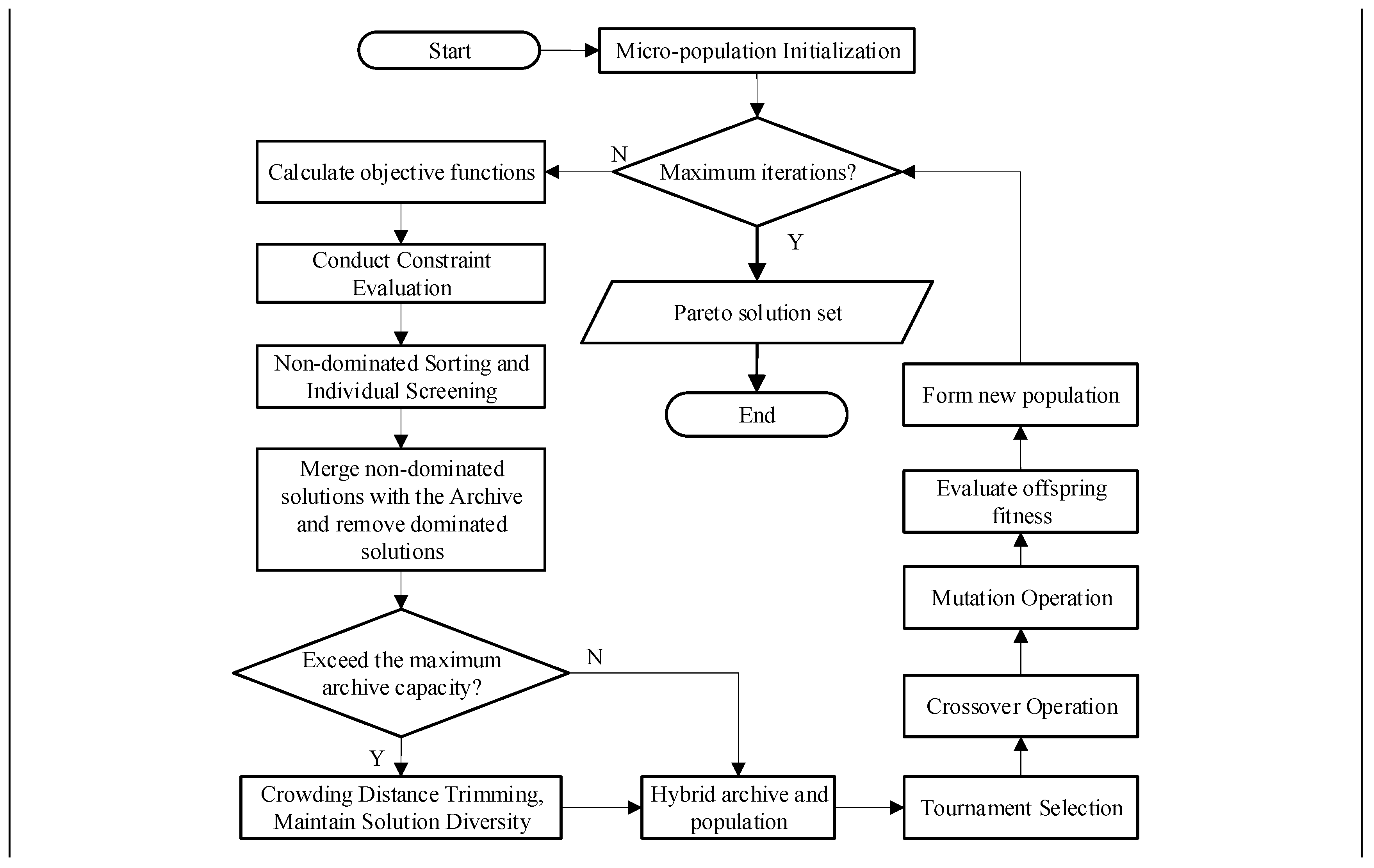
Figure 14.
Multiple-objective optimization Flowchart.
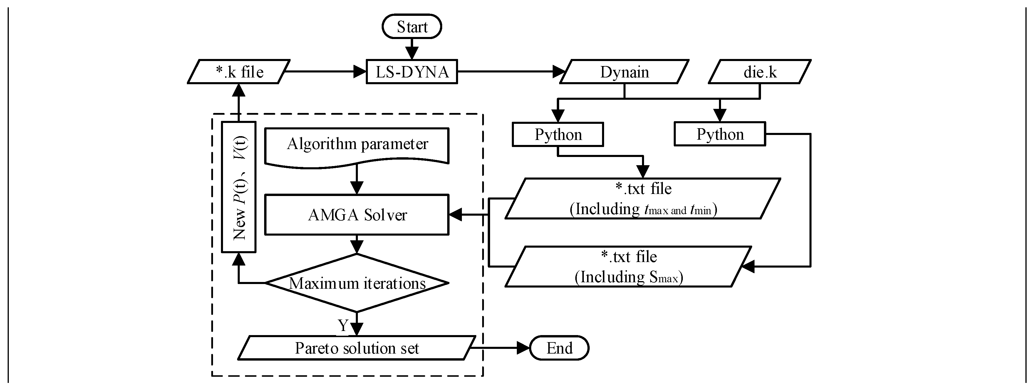
Figure 15.
Scatter diagram of Pareto optimal solutions.
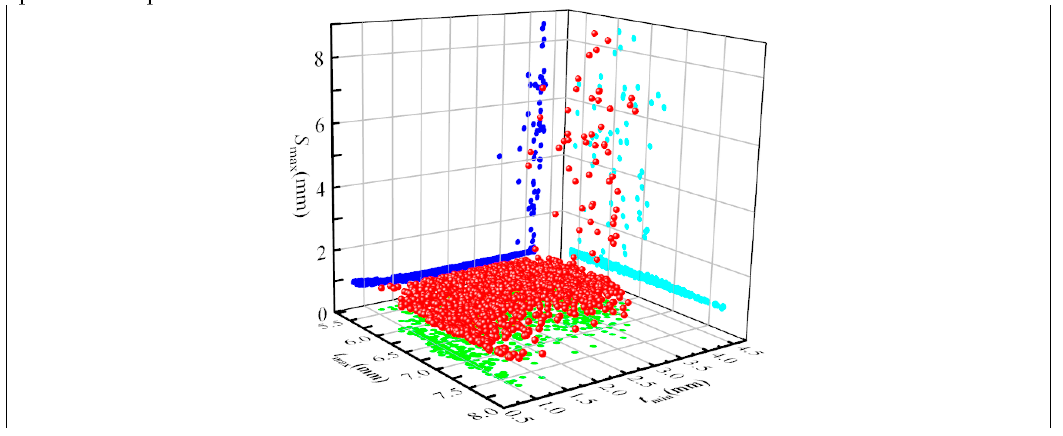
Figure 16.
Variation of maximum and minimum wall thickness with iterations.
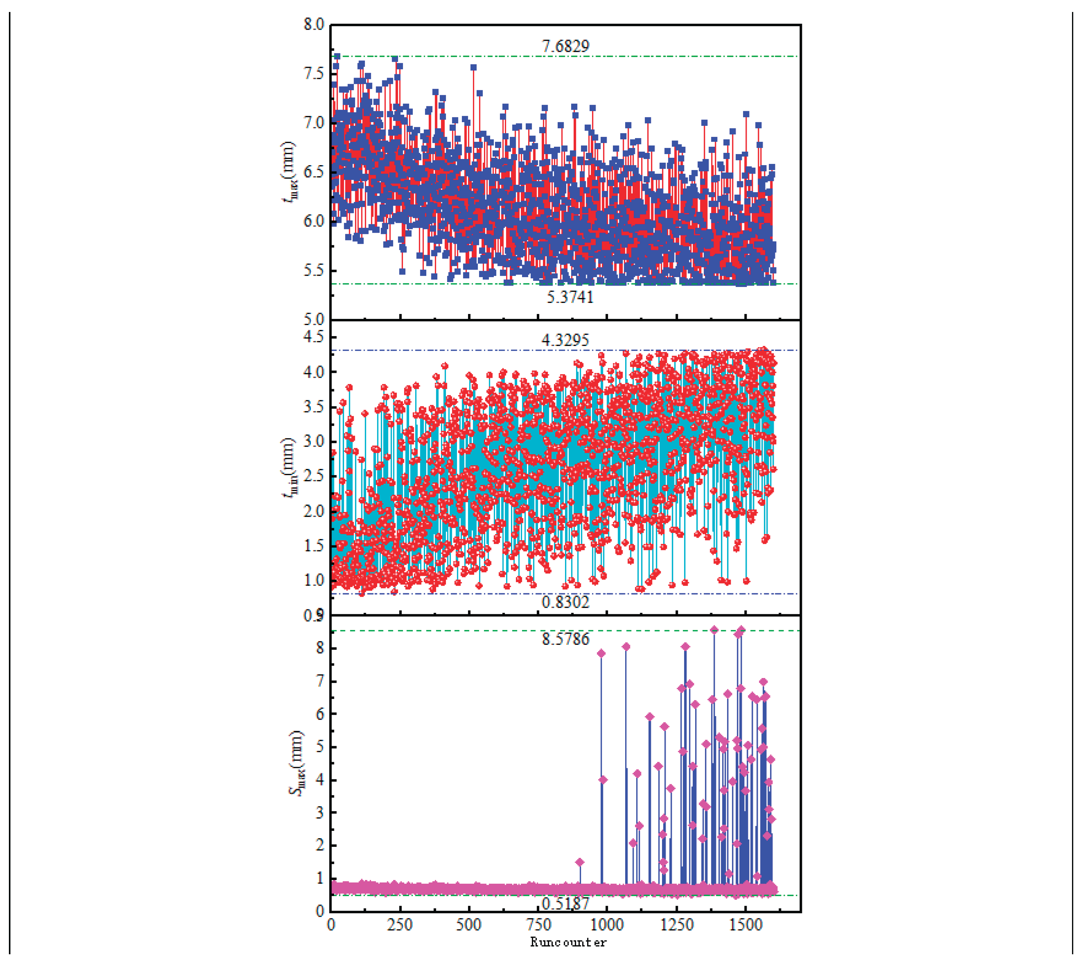
Figure 17.
Three-objective Pareto optimal front and its two-dimensional projections.
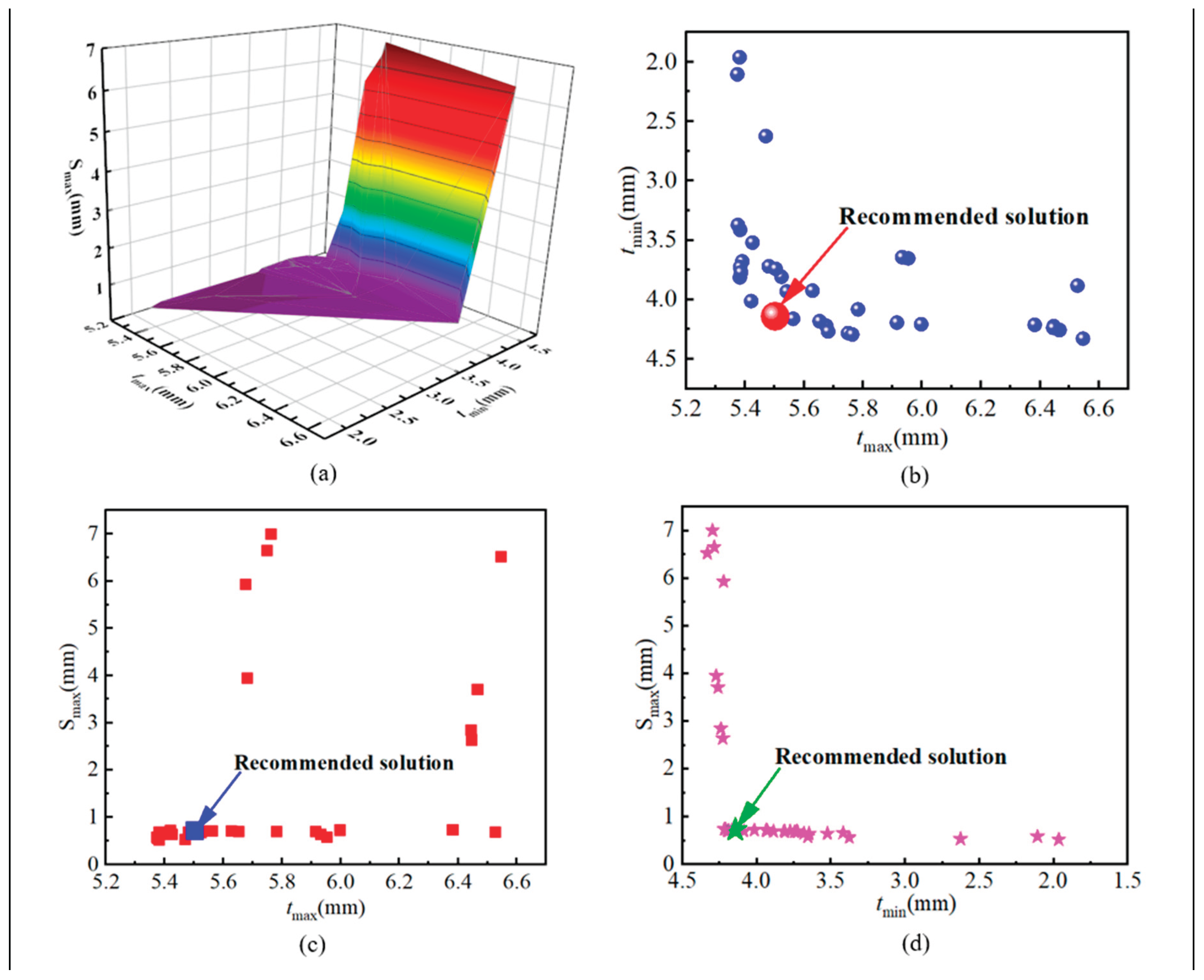
Figure 18.
Pareto solutions under different maximum gap conditions: (a) Smax=0.73mm, (b) Smax=1.09mm, (c) Smax=2.0mm.
Figure 18.
Pareto solutions under different maximum gap conditions: (a) Smax=0.73mm, (b) Smax=1.09mm, (c) Smax=2.0mm.
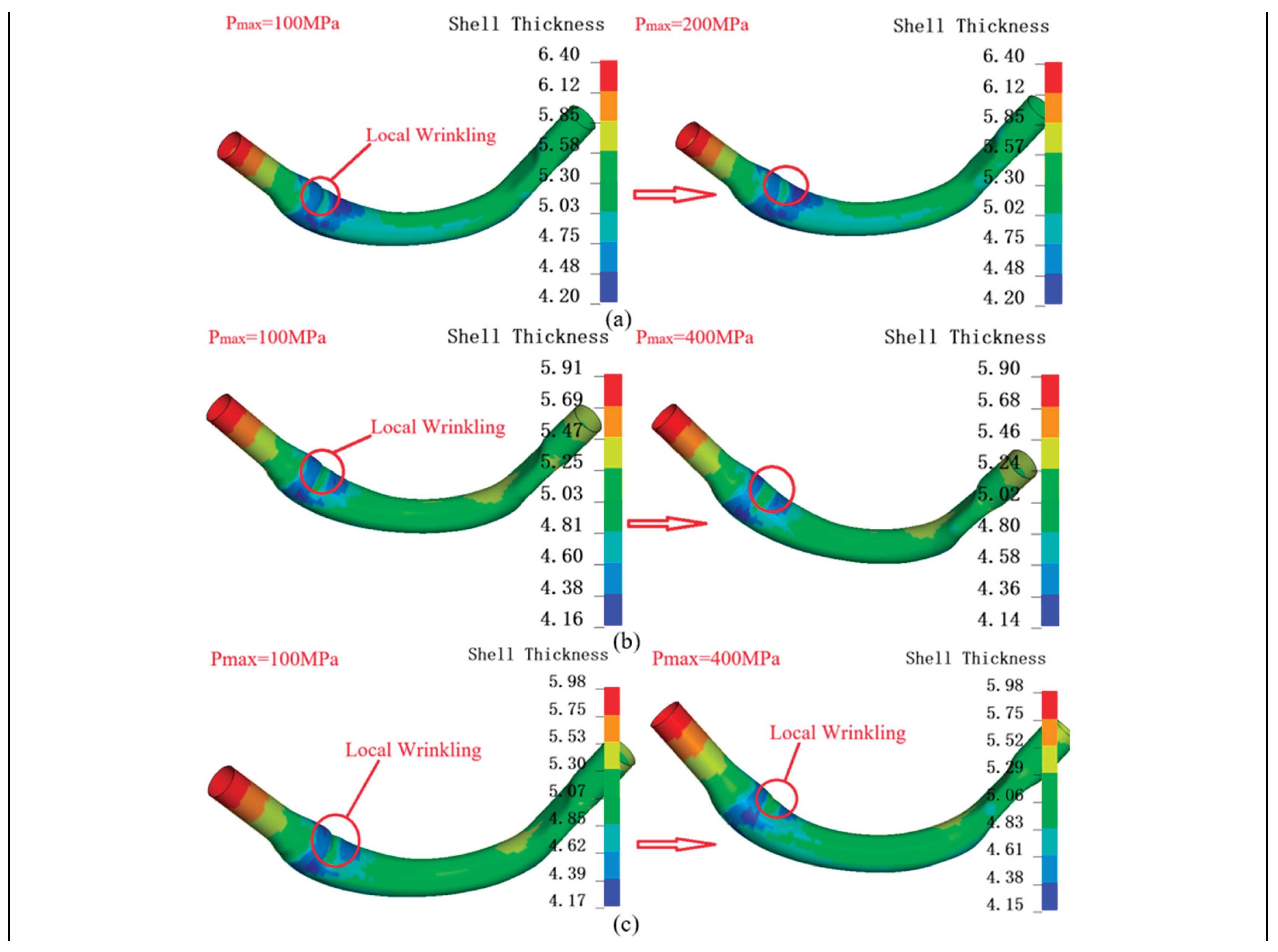
Figure 19.
Comparison of all feasible solutions and feasible solutions in Pareto set: (a) All feasible process solutions of simulation results, (b) Feasible process solutions in Pareto optimal solutions.
Figure 19.
Comparison of all feasible solutions and feasible solutions in Pareto set: (a) All feasible process solutions of simulation results, (b) Feasible process solutions in Pareto optimal solutions.
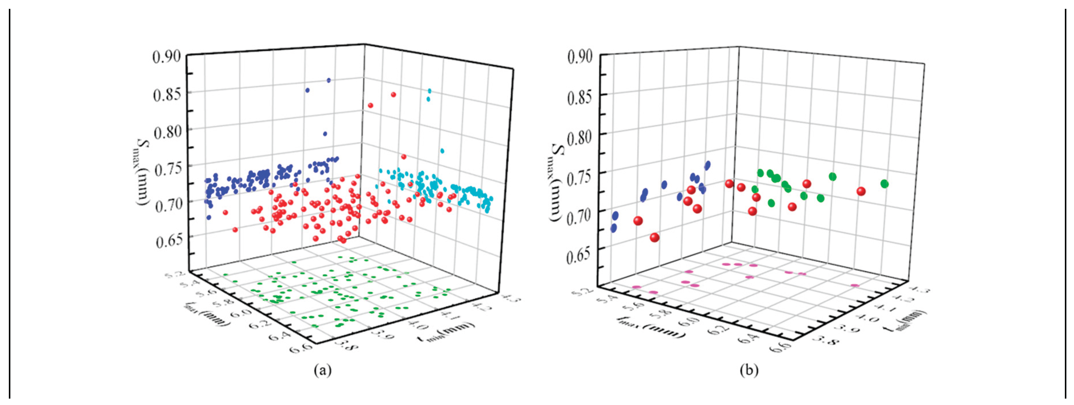
Figure 20.
Pareto optimal solutions under constrained conditions.
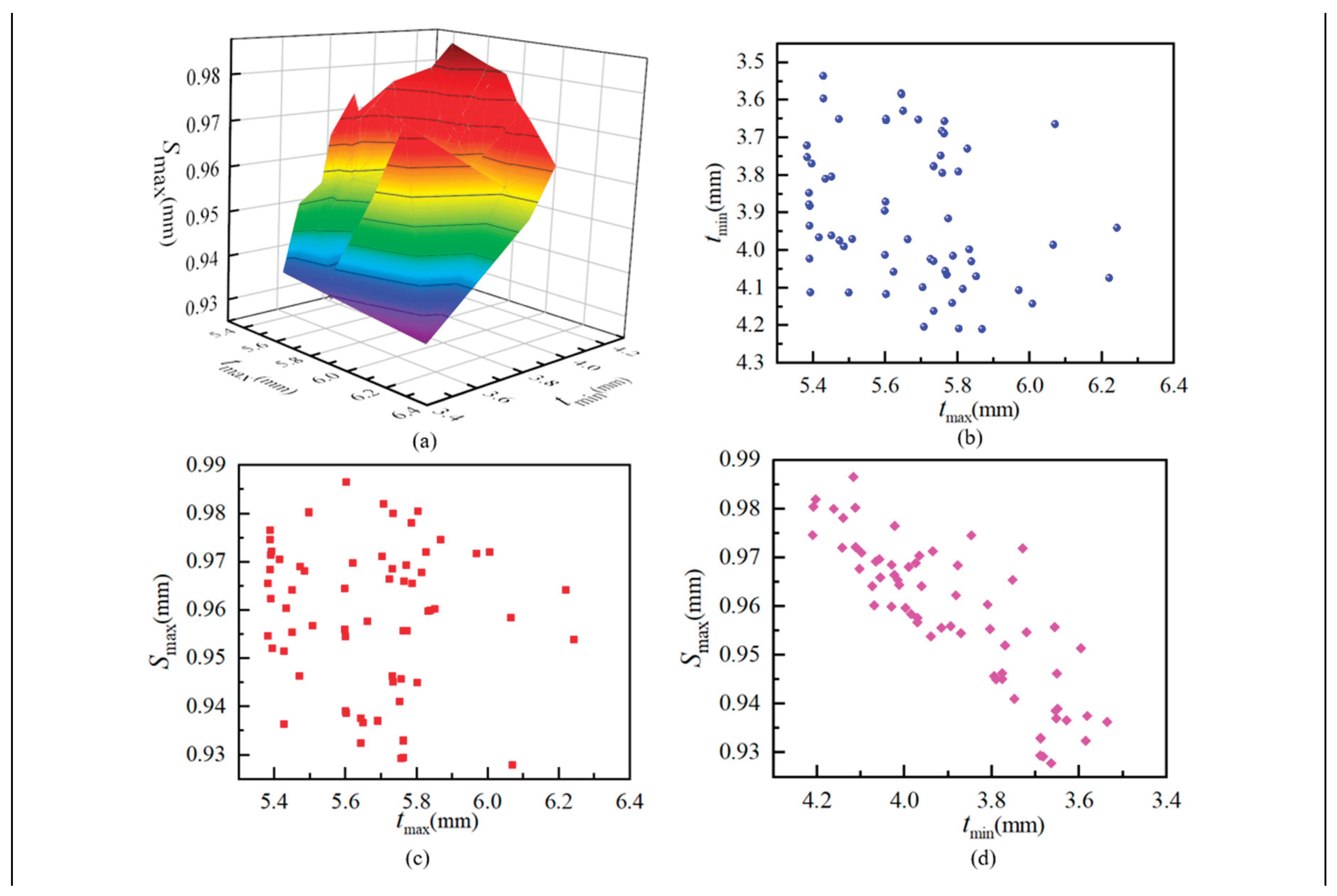
Figure 21.
Correlation between partial design variables and optimization objectives.
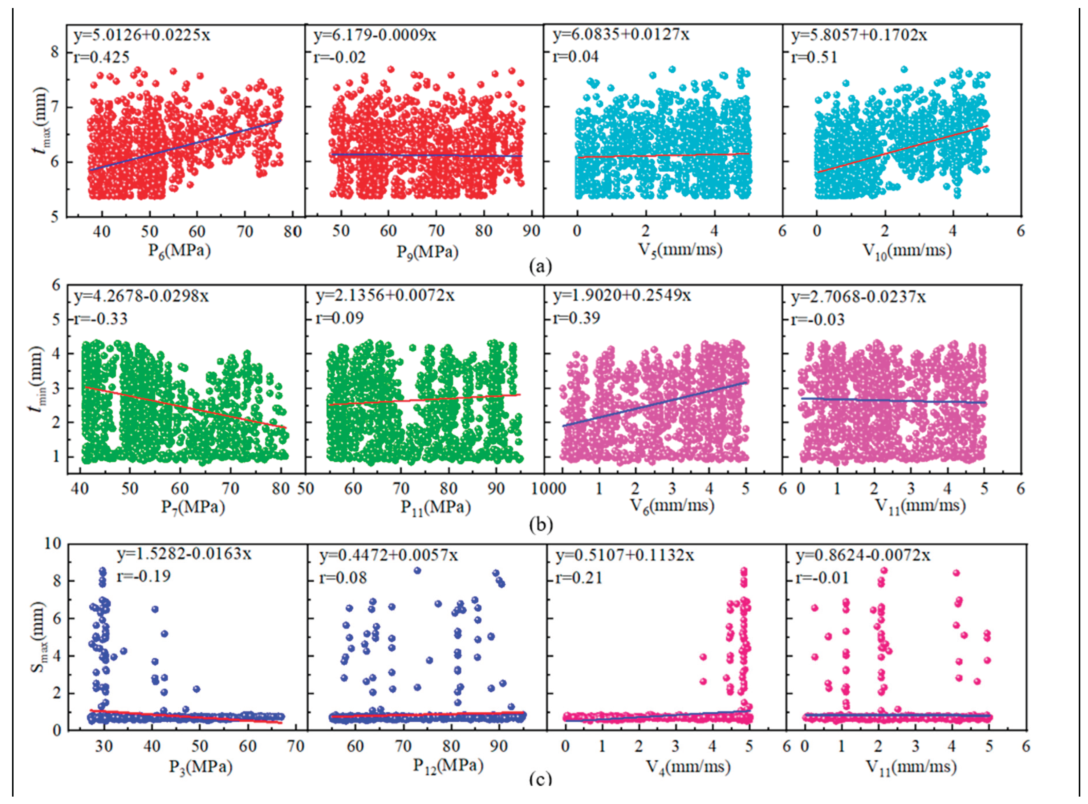
Figure 22.
Pressure curve and feed velocity curve under three schemes.
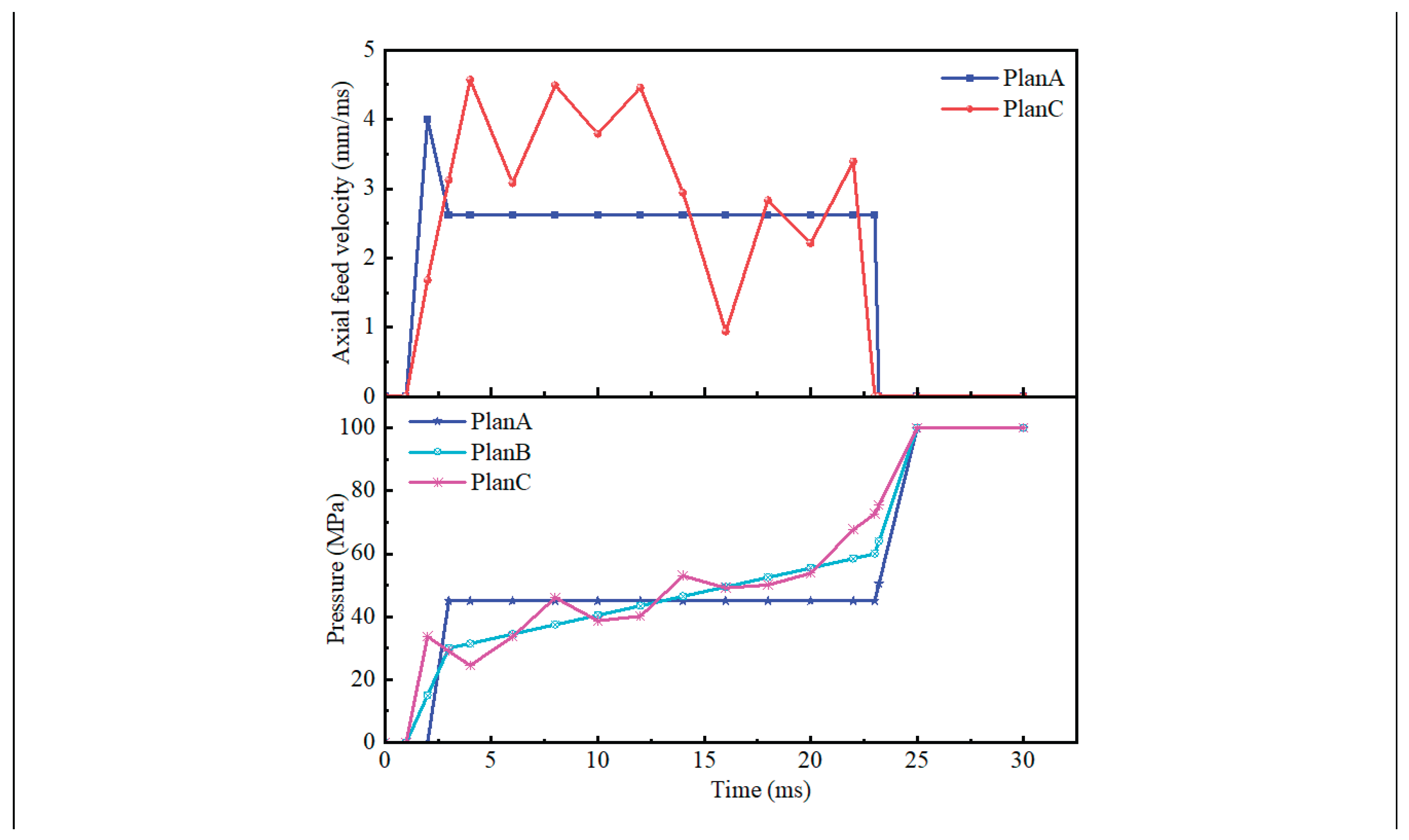
Figure 23.
Simulation results using different process plans: (a) plan A, (b) plan B, (c) plan C.
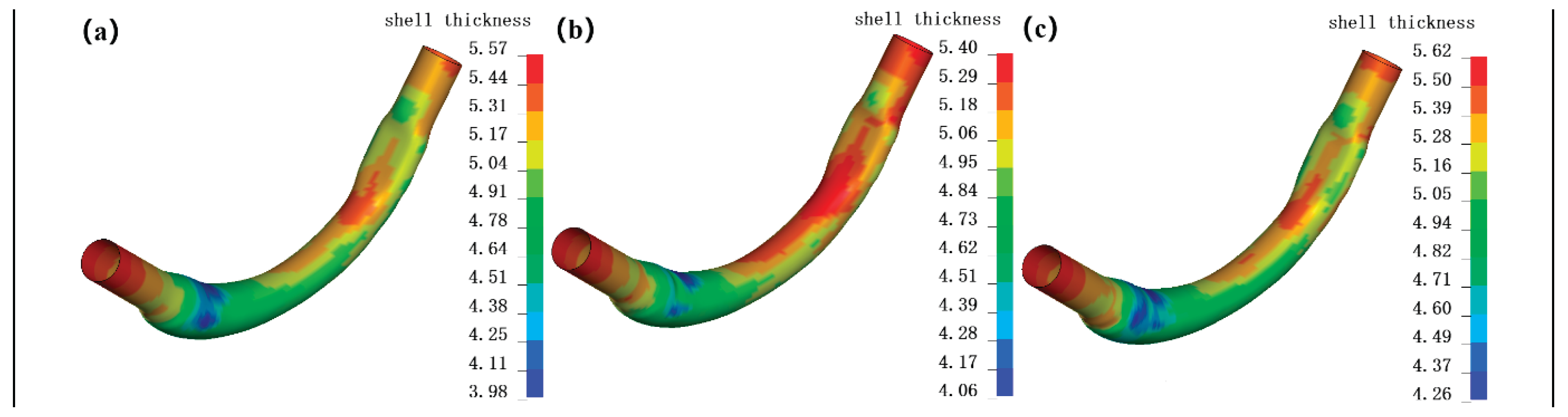
Figure 24.
Simulation results using different process plans.
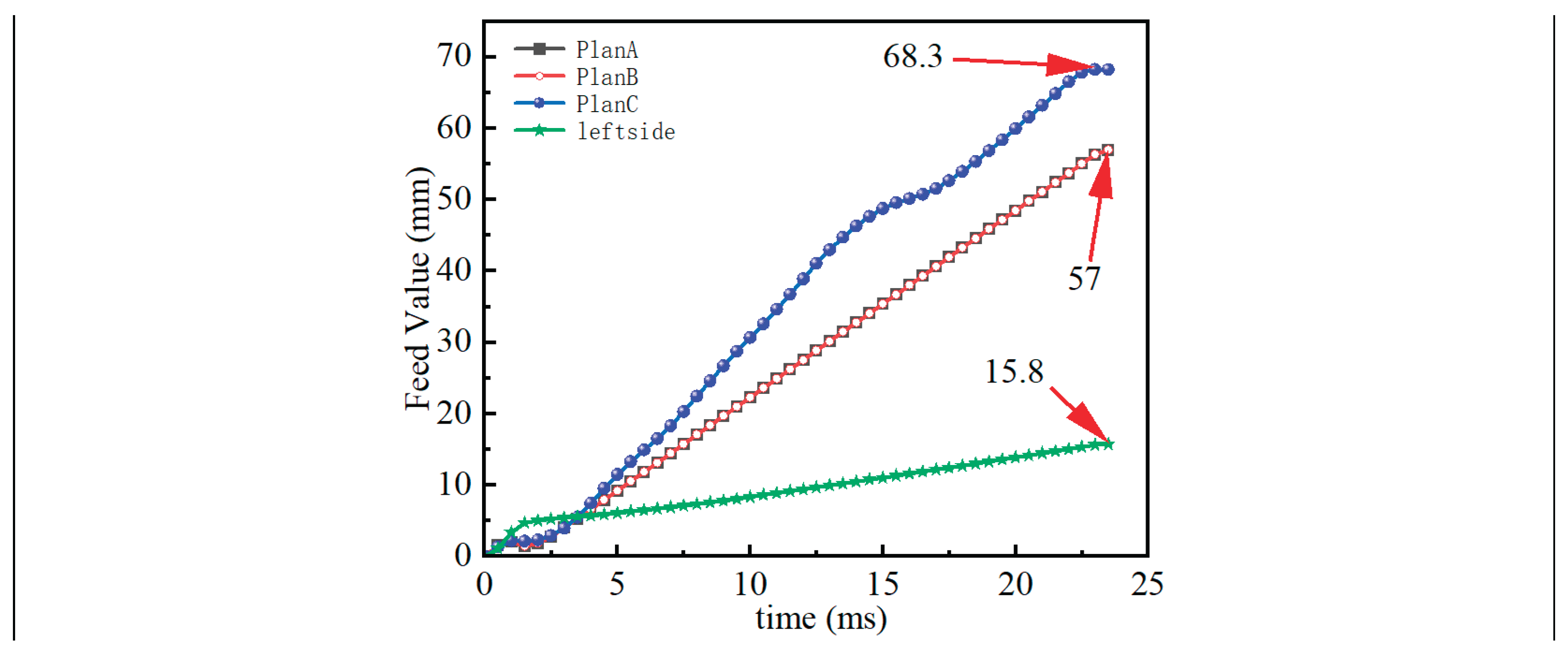

Table 1.
Table of correspondence between element size and simulation results.
| Element size | Work step | Elementnumber | Simulation time | ||
| Calculation time | Tmax | Tmin | |||
| 2mm | Pre-bending | 63862 | 51min52s | 5.37 | 4.62 |
| Pre-forming | 95965 | 42min1s | 5.39 | 4.62 | |
| Hydroforming | 102054 | 74min35s | 5.58 | 3.99 | |
| 4mm | Pre-bending | 30838 | 12 min | 5.49 | 4.62 |
| Pre-forming | 24059 | 3min21s | 5.52 | 4.63 | |
| Hydroforming | 27450 | 6m19s | 5.60 | 3.97 | |
| 6mm | Pre-bending | 24694 | 7min50s | 5.29 | 4.57 |
| Pre-forming | 10736 | 37s | 5.52 | 4.55 | |
| Hydroforming | 13694 | 1min6s | 5.57 | 3.98 | |
Table 2.
Statistics of simulation prediction deviation at each measuring point of transverse section.
Table 2.
Statistics of simulation prediction deviation at each measuring point of transverse section.
| Measuring point | Section A | Section B | Section C | Section D | Section E |
| T1 | -2.95% | -4.6% | -3.86% | -3.08% | -6.97% |
| T2 | 0.24% | -4.1% | -4.82% | -2.12% | -6.45% |
| T3 | 0.16% | 1.41% | -3.08% | 0.46% | -3.1% |
| T4 | 0.4% | -2.06% | -5.23% | 0.21% | -2.78% |
| T5 | -3.83% | -7.16% | -4.49% | -1.18% | -6.77% |
| T6 | -2.72% | -3.99% | -5.55% | -4.92% | -2.95% |
| T7 | -4.55% | -7.31% | -6.91% | -6.57% | -3.14% |
| T8 | -3.07% | -7.46% | -4.58% | 2.23% | -2.3% |
Table 3.
The correlation coefficients between design variables and optimization objectives.
| Variables | P1 | P2 | P3 | P4 | P5 | P6 | P7 | P8 | P9 | P10 | P11 | P12 |
| 0.16 | 0.28 | 0.18 | 0.25 | 0.09 | 0.43 | 0.40 | 0.32 | -0.02 | 0.19 | 0.19 | 0.18 | |
| -0.28 | -0.002 | -0.18 | 0.04 | -0.22 | -0.27 | -0.33 | -0.14 | -0.17 | -0.11 | 0.09 | -0.13 | |
| -0.11 | 0.02 | -0.19 | 0.02 | -0.13 | -0.04 | -0.13 | -0.10 | -0.17 | 0.01 | 0.04 | 0.08 | |
| Variables | V1 | V2 | V3 | V4 | V5 | V6 | V7 | V8 | V9 | V10 | V11 | |
| 0.29 | 0.24 | 0.22 | 0.10 | 0.04 | 0.06 | 0.18 | 0.33 | 0.43 | 0.51 | 0.19 | ||
| 0.16 | 0.17 | 0.27 | 0.38 | 0.30 | 0.39 | 0.26 | 0.27 | 0.13 | -0.03 | -0.03 | ||
| 0.05 | 0.19 | 0.17 | 0.21 | 0.18 | 0.16 | 0.12 | 0.14 | 0.17 | 0.02 | -0.01 |
Disclaimer/Publisher’s Note: The statements, opinions and data contained in all publications are solely those of the individual author(s) and contributor(s) and not of MDPI and/or the editor(s). MDPI and/or the editor(s) disclaim responsibility for any injury to people or property resulting from any ideas, methods, instructions or products referred to in the content. |
© 2026 by the authors. Licensee MDPI, Basel, Switzerland. This article is an open access article distributed under the terms and conditions of the Creative Commons Attribution (CC BY) license (http://creativecommons.org/licenses/by/4.0/).
Copyright: This open access article is published under a Creative Commons CC BY 4.0 license, which permit the free download, distribution, and reuse, provided that the author and preprint are cited in any reuse.


