

Submitted:
23 June 2026
Posted:
24 June 2026
You are already at the latest version
Abstract
Urban green spaces are increasingly recognized as multifunctional cooling infrastructure for climate resilience, environmental health, and spatial equity. However, the potential contributions of green spaces depends not only on their location, but also on whether their cooling benefits are realized and aligned with heat-sensitive demand. This study develops a spatially explicit cooling-service framework to examine green-space cooling supply, thermal regulation, human-relevant thermal pressure, and cooling-service mismatch across 1,385 census tracts in Maryland, USA. A Landscape Cooling Supply Index (LCSI) was constructed from vegetation coverage, tree canopy, park provision, water-area proportion, impervious surface, and road infrastructure indicators. Fixed-effects regression models were used to test associations between LCSI and multiple thermal outcomes, including land surface temperature, Heat Index, extreme hot days, and an integrated Human-Relevant Thermal Pressure Index (HTPI). XGBoost and SHAP were applied to identify nonlinear contributions of green, blue, and gray components to thermal pressure. A Heat-sensitive Cooling Demand Index was then developed to classify cooling supply-demand mismatch. Results show that stronger cooling supply is significantly associated with lower surface and human-relevant thermal pressure. Explainable GeoAI results identify overall vegetation coverage as the dominant green component, while water-area proportion and road-related gray infrastructure also play important roles. The mismatch analysis identifies 433 census tracts, or 31.3% of all Maryland tracts, as low-supply–high-demand priority areas. This study provides a tract-level framework for targeting green-space cooling interventions where climate exposure, environmental health vulnerability, and cooling-service inequity converge.
Keywords:
green space
; landscape ecosystem
; thermal environment
; heat pressure
; climate resilience
; emergency management
1. Introduction
As extreme heat becomes a more persistent feature of urban and regional climate risk, urban green spaces are increasingly being repositioned as infrastructure for adaptation rather than as residual open land or recreational amenities alone (Marketaki et al., 2026; Butt & Rigoni, 2025; Meerow & Newall, 2017; Norton et al., 2015). This shift is important for land-use planning because the capacity to cope with heat depends not only on meteorological conditions, but also on how vegetated areas, tree canopy, parks, water bodies, impervious surfaces, road networks, and residential populations are arranged across space. Green spaces can moderate heat through shading, evapotranspiration, reduced surface heat storage, and the creation of cooler outdoor environments (Bowler et al., 2010; Ziter et al., 2019). At the same time, their cooling functions are conditioned by adjacent blue spaces and by heat-amplifying gray infrastructure, including impervious surfaces and road networks (Oke, 1982; Voogt & Oke, 2003; Weng, 2009). Treating green spaces as multifunctional cooling infrastructure therefore requires an analytical framework that connects ecological cooling capacity with thermal outcomes, human exposure, and uneven social needs.
This infrastructural perspective is further clarified through the concept of blue–green infrastructure (BGI). BGI has been widely used to describe interconnected networks of natural, semi-natural, and water-related landscape components that provide multiple ecosystem, climate, public-health, and social benefits across urban systems (Liu et al., 2026; Campbell et al., 2024; Siehr et al., 2022). A census tract may contain designated parkland but still have limited cooling capacity if park areas are dominated by impervious surfaces, sparse canopy, or fragmented vegetation. Conversely, cooling benefits may be generated by tree canopy, vegetated land, wetlands, riparian corridors, or other non-park landscapes that are not always captured by formal park indicators. Water bodies may further contribute to localized cooling, while roads and impervious surfaces can intensify heat storage and disrupt the continuity of cooling landscapes. For this reason, green-space cooling infrastructure should be evaluated as part of a broader blue–green–gray system. In this study, the Landscape Cooling Supply Index (LCSI) is retained as the operational measure of this cooling-infrastructure function: it captures the relative balance between cooling-supportive green/blue components and heat-amplifying gray infrastructure.
Evaluating green spaces as cooling infrastructure also requires moving from potential supply to realized thermal regulation. Ecosystem service and land use planning research has long emphasized that ecological structures become socially meaningful when their functions generate benefits and respond to demand (Burkhard et al., 2012; Haines-Young & Potschin, 2010). In the context of urban heat adaptation, this means that vegetation coverage, park area, and green-space accessibility should not be assumed to produce equivalent cooling benefits across all neighborhoods. These indicators are valuable, but they cannot by themselves demonstrate whether stronger cooling supply corresponds to lower thermal pressure. The relationship between green-space structure and urban heat is mediated by land-cover composition, surface properties, humidity, urban morphology, background climate, and scale of analysis (Li et al., 2023; Rahimi et al., 2021; Zhou & Wang, 2011). Therefore, a planning-relevant assessment needs to test whether areas with stronger cooling-supportive composition experience lower heat outcomes after accounting for broader spatial context.
A further complication is that urban heat has multiple causes (Jabbar et al., 2023; Karimi et al., 2023). Land surface temperature is indispensable for assessing surface energy balance and the response of built and vegetated surfaces to solar radiation (Voogt & Oke, 2003; Weng, 2009). However, surface temperature is not equivalent to the heat stress experienced by residents. Human-relevant thermal pressure depends on apparent temperature, humidity, repeated hot days, housing conditions, behavioral exposure, and adaptive resources (Anderson et al., 2013; Harlan & Ruddell, 2011). For example, a tract with moderate surface temperature may still experience substantial heat-health pressure if high humidity and frequent extreme heat days coincide with vulnerable populations. Conversely, a high-LST tract may not always represent the highest human exposure burden. Green-space cooling research therefore needs to distinguish surface-oriented thermal regulation from indicators that more directly capture environmental health relevance.
The equity dimension of green-space cooling infrastructure is equally important. Cooling services become socially consequential when they reach the places and populations that need them most. Prior studies have shown that heat exposure, urban heat-island intensity, and heat-risk-related land-cover conditions are unevenly distributed across racial, socioeconomic, and neighborhood groups (Peng et al., 2025; Chakraborty et al., 2019; Hsu et al., 2021; Jesdale et al., 2013). At the same time, access to green-space and its associated health benefits are shaped by environmental justice, social determinants of health, and the uneven distribution of urban greening (Jennings & Johnson Gaither, 2015; Kabisch et al., 2015; Wolch et al., 2014). These findings suggest that evaluating the public value of green-space cooling requires more than the size, type and number of green spaces. Heat-related demand in terms of how much people need relief from heat is determined by a mix of factors, including the overlap of thermal pressure, age-related susceptibility, social isolation, socioeconomic disadvantage, limited health-care access, and constrained household adaptation such as lack of air conditioning (Guardaro et al. 2022). If green-space cooling supply is concentrated in areas with lower heat-health demand, while vulnerable communities face weaker cooling supply, then green infrastructure may reproduce rather than reduce spatial inequity.
This concern is especially relevant because urban greening is not automatically equitable. New parks, tree-planting programs, greenways, and waterfront improvements may improve environmental quality, but they can also generate uneven benefits if they are not aligned with the needs of historically underserved or heat-sensitive communities (Anguelovski et al., 2018; Wolch et al., 2014). Therefore, the key planning question is not simply whether green spaces cool urban environments, but whether cooling benefits are spatially aligned with heat-health demand. A cooling-service equity perspective requires identifying where low cooling supply coincides with high heat-sensitive demand and where interventions such as tree-canopy expansion, vegetation restoration, blue–green corridor enhancement, park redesign, and gray-surface retrofitting may generate the greatest adaptation value.
Three gaps motivate the present study. First, existing work often evaluates green-space amount, vegetation cover, or landscape composition as proxies for cooling capacity, without sufficiently validating whether such supply corresponds to realized thermal outcomes. Second, studies frequently privilege land surface temperature while giving less attention to apparent heat and recurrent extreme heat exposure, even though these indicators are more directly connected to human thermal burden. Third, research on green-space equity often documents unequal access or unequal exposure, but less often integrates cooling supply, realized thermal regulation, environmental-health demand, and spatial mismatch within one tract-level framework. These gaps limit the ability of planners to identify not only where green infrastructure exists, but where additional cooling investment is most needed.
Responding to these limitations, this study examines urban green spaces as multifunctional cooling infrastructure across 1,385 census tracts in Maryland, USA. Maryland provides a suitable setting because it contains pronounced variation in urbanization, vegetation, park provision, water coverage, road infrastructure, and population vulnerability within one state-level planning context. The Baltimore–Washington corridor is densely developed with extensive gray infrastructure. In contrast, other suburban and agricultural areas in Maryland such as along the Eastern Shore, the Chesapeake Bay region and the mountainous part of western provide a wide range of contrasting blue and green landscape conditions. This spatial diversity makes it possible to evaluate whether green-space cooling supply operates consistently across heterogeneous urban, suburban, coastal, and rural settings.
The analysis of green-space cooling infrastructure is organized around four questions. First, how can the cooling-infrastructure function of urban green spaces be quantified for census tracts while accounting for green, blue, and gray components? Second, is LCSI linked to realized thermal regulation measured by maximum land surface temperature, Heat Index, extreme hot days, and an integrated Human-Relevant Thermal Pressure Index? Third, which green, blue, and gray components have the strongest and most nonlinear contributions to human-relevant thermal pressure? Fourth, where do low cooling supply and high heat-sensitive demand coincide, and which tracts should be prioritized from a cooling-service equity perspective?
Empirically, the study constructs LCSI to represent green-space cooling supply within a blue–green–gray infrastructure system; tests its association with multiple thermal outcomes using fixed-effects regression; applies XGBoost and SHAP to identify nonlinear component-level contributions to human-relevant thermal pressure; and develops a Heat-sensitive Cooling Demand Index and mismatch typology to locate low-supply–high-demand priority areas. By linking thermal regulation, environmental health, and cooling-service equity, the study advances three contributions. Conceptually, it reframes urban green spaces as multifunctional infrastructure for heat adaptation. Methodologically, it connects cooling supply, realized thermal outcomes, human-relevant heat pressure, and demand-side vulnerability in a single spatial framework. Practically, it offers a tract-level diagnostic approach for targeting green-space cooling interventions where climate exposure, health sensitivity, and infrastructure deficits converge.
2. Literature Review
2.1. Urban Green Spaces as Multifunctional Cooling Infrastructure
Urban green spaces are increasingly recognized as multifunctional infrastructure for climate adaptation, local climate regulation, and human well-being (Athokpam et al. 2024; Harath & Bai, 2024; Kim & Song, 2019). Their cooling function is produced through multiple biophysical pathways, including shading, evapotranspiration, reduced heat storage, and modification of surface–atmosphere exchange. However, the cooling capacity of green spaces depends not only on the amount of vegetation or parkland, but also on how green, blue, and gray elements are combined within urban landscapes. From a landscape ecological perspective, this reflects the broader pattern–process relationship: spatial composition and configuration shape ecological processes, including urban thermal regulation (Oke, 1982; Turner, 1989).
Studies using landscape metrics have shown that both landscape composition and configuration are associated with LST, although their effects may vary by spatial scale, metric selection, and urban context. Zhou et al. demonstrated that land-cover composition and spatial configuration both matter for explaining LST in urban landscapes (Zhou et al., 2011). Rahimi et al. further showed that the relationship between urban landscape heterogeneity and LST is scale-dependent, indicating that landscape–thermal relationships cannot be fully captured by a single spatial scale or metric (Rahimi et al., 2021). A recent systematic review of urban green-space configuration similarly concluded that larger, more aggregated, and more complex-shaped green spaces often generate stronger cooling effects, while also noting that empirical findings differ across cities, metrics, and methodological designs (Li et al., 2023). These studies establish landscape pattern–thermal regulation as a mature research field, while also highlighting the need to select indicators that match the spatial unit, data availability, and analytical purpose of a given study.
Vegetation is one of the most widely studied green-space cooling components in urban thermal regulation. Its cooling effect is usually explained through shading, evapotranspiration, reduced surface heat storage, and modification of near-surface microclimate. Systematic evidence suggests that urban greening generally lowers local temperatures, although the magnitude of cooling varies by vegetation type, spatial extent, background climate, and measurement method (Bowler et al., 2010). Tree canopy is especially important because it can directly reduce solar radiation reaching built surfaces and pedestrians. Ziter et al. showed that tree canopy and impervious surface interact in scale-dependent ways to influence daytime summer heat, implying that vegetation effects should be assessed together with heat-amplifying urban surfaces rather than in isolation (Ziter et al., 2019). For this reason, indicators such as vegetation coverage and tree-canopy coverage are often used to represent the green components of landscape cooling supply.
Water bodies constitute another important component of urban thermal regulation. Blue spaces can contribute to local cooling through evaporative processes, high heat capacity, and the creation of cooler surface conditions relative to surrounding built-up areas. In landscape-based heat adaptation studies, water coverage is therefore commonly treated as a cooling-supportive element, especially in regions where rivers, bays, wetlands, reservoirs, or coastal landscapes form a substantial part of the local environment. However, the effect of water is also spatially contingent: its cooling contribution depends on size, exposure, surrounding land cover, and the degree to which nearby populations or built environments are connected to blue-space cooling effects. This makes water-area proportion a meaningful landscape indicator for evaluating cooling supply at neighborhood or census-tract scales.
In contrast, impervious surfaces and road characteristics represent gray infrastructure that tend to amplify thermal pressure. Impervious surfaces store and re-radiate heat, reduce evapotranspiration, and are often associated with dense built environments, while roads contribute to heat absorption, traffic-related anthropogenic heat, and the fragmentation of cooling landscape elements. Prior research has repeatedly shown that impervious cover is positively associated with higher urban temperatures and can weaken or offset the cooling contribution of tree canopy and other vegetation (Ziter et al., 2019). Road length and road density can therefore be interpreted not merely as transportation indicators, but as proxies for linear gray infrastructure that may intensify or redistribute urban thermal pressure. Including these indicators helps distinguish cooling-supportive landscape elements from heat-amplifying infrastructure.
Parks occupy a more ambiguous position in urban thermal regulation. On the one hand, parks are important providers of recreational, cultural, and potentially cooling ecosystem services. Larger parks or more spatially aggregated green spaces may generate stronger cooling islands and influence surrounding thermal environments (Li et al., 2023). On the other hand, formal park provision does not necessarily equal vegetation-based cooling function. Park boundaries may include lawns, paved surfaces, water bodies, tree canopy, sports facilities, buildings, and other mixed land-cover types. As a result, park area, park proportion, and park area per capita are better interpreted as indicators of formal green-space provision, while vegetation coverage and tree canopy more directly represent the biophysical components that drive cooling processes. This distinction is important for assessing whether planned green-space supply translates into realized thermal regulation. Therefore, this study treats LCSI not as a simple green-space quantity measure, but as an operational index of green-space cooling infrastructure within a blue–green–gray system.
2.2. Green Space Cooling and Human-relevant Thermal Pressure
A body of research has linked green infrastructure, urban heat mitigation, and health-relevant exposure. For example, studies of urban green infrastructure have shown that tree canopy and other green elements can reduce extreme surface temperatures and may contribute to heat-risk mitigation for vulnerable populations (Venter et al., 2020). However, much of the inequality literature focuses on who is exposed to more heat, who receives fewer cooling benefits, or how heat burdens differ across social groups. These are essential questions for environmental justice, but they do not always explain the landscape ecological process through which cooling supply is produced, how it translates into realized thermal regulation, or why it may fail to match demand. In other words, cooling inequality has been well established as a distributional problem, but it remains less fully connected to the pattern–process logic of landscape ecology and the supply–demand logic of ecosystem services.
This gap is partly related to how urban heat is measured. Land surface temperature is widely used because it is spatially continuous, remotely sensed, and closely linked to surface energy balance. It is therefore highly useful for assessing surface thermal conditions and landscape-driven surface thermal regulation. However, LST should not be treated as equivalent to human heat exposure or human thermal comfort. Prior work has cautioned that surface temperature alone may not adequately represent the thermal conditions experienced by people at street level, where humidity, shade, wind, radiation, and activity patterns also matter (Turner et al., 2022). Therefore, a landscape that reduces LST may not necessarily reduce human-perceived heat pressure to the same extent, and an area with high surface temperature may not always correspond to the highest human-relevant thermal burden.
For this reason, this study distinguishes among three types of thermal outcomes. First, LSTmax is used to represent surface thermal condition and surface-oriented thermal regulation. Second, Heat Index is used to capture human-perceived heat pressure because it combines air temperature and humidity into an apparent temperature metric commonly used in environmental health research (Anderson et al., 2013; Rothfusz, 1990). Third, extreme hot days are used to represent the frequency of extreme heat exposure, reflecting the cumulative or recurrent nature of heat stress rather than a single thermal snapshot (Perkins, 2015). This distinction is important because the relationship between landscape cooling supply and thermal conditions may differ depending on whether heat is measured as surface temperature, perceived heat pressure, or extreme heat frequency. Environmental health relevance also has an equity dimension because heat exposure and cooling benefits are unevenly distributed across social groups. At the global scale, recent evidence shows that urban green spaces provide substantial cooling, but the magnitude of cooling capacity and resident-level cooling benefit varies strongly across world regions and cities (Li et al., 2024). This suggests that cooling inequality is not merely a matter of whether green space exists, but also whether cooling benefits are spatially aligned with where people live and experience heat. At the intra-urban scale, studies in the United States and other urban contexts have shown that low-income populations, people of color, and racially segregated communities are often exposed to higher levels of urban heat or heat-risk-related land-cover conditions (Benz & Burney, 2021; Chakraborty et al., 2019; Hsu et al., 2021; Jesdale et al., 2013). Together, these studies establish that cooling inequality and heat exposure inequality are already well documented across global, national, and intra-urban scales.
2.3. Cooling Service Equity and Supply–Demand Mismatch
A cooling-service equity perspective requires moving beyond the question of whether green spaces provide cooling capacity toward the question of whether such capacity is spatially aligned with heat-sensitive demand. Burkhard et al. established an influential spatial framework for mapping ecosystem service supply, demand, and budgets, showing that service provision cannot be assessed only from the supply side (Burkhard et al., 2012). Later studies further emphasized that mismatches may arise when ecosystem service capacity is spatially separated from demand, when demand exceeds local supply, or when potential services are not effectively delivered to populations who need them (Geijzendorffer et al., 2015; Villamagna et al., 2013; Wolff et al., 2015). This supply–demand perspective is particularly relevant for urban cooling services because heat mitigation is both spatially produced by landscape elements and socially needed by exposed or sensitive populations.
In the context of urban thermal regulation, the supply–demand framework challenges a simple assumption: more green space does not necessarily mean sufficient cooling service, and stronger cooling capacity does not necessarily mean better alignment with heat-sensitive demand. From an equity perspective, low-supply–high-demand areas are not only service-deficit areas, but also priority areas for green-space cooling intervention. Syrbe et al. proposed a national indicator of local climate regulation in German cities that explicitly relates green infrastructure cooling capacity to residential demand, thereby moving beyond the evaluation of green-space quantity alone (Syrbe et al., 2024). This type of approach is important because cooling service should be assessed not only as an ecological function, but also as a spatially distributed benefit that may or may not reach populations experiencing thermal pressure.
Recent studies have begun to apply this logic more directly to cooling services. Wang et al. examined the matching relationship between cooling supply and demand provided by urban green and blue spaces and showed that four-quadrant analysis and bivariate LISA can be used as complementary tools for identifying areas with different supply–demand states, especially low-supply and high-demand areas requiring planning attention (Wang et al., 2024). Related studies on park cooling and accessibility have also shown that cooling effects may be unevenly distributed and may not be accessible to all neighborhoods during extreme heat events (Chen et al., 2022). These findings suggest that cooling-service assessment needs to move beyond measuring total green or blue space area and instead evaluate whether cooling resources are spatially matched with thermal exposure and vulnerable demand.
Methodologically, cooling supply–demand mismatch is commonly assessed through several complementary approaches. The first is index-based assessment, in which cooling supply and cooling demand are separately quantified through standardized indicators and then compared. This approach is useful for constructing spatially explicit supply and demand surfaces, but it depends heavily on indicator selection and weighting. The second is quadrant-based typology, which classifies spatial units into high-supply–low-demand, high-supply–high-demand, low-supply–low-demand, and low-supply–high-demand types. Among these, low-supply–high-demand areas are interpreted as cooling-service equity priority areas, where green-space enhancement, tree-canopy expansion, blue–green corridor improvement, and gray-surface retrofitting should have the greatest planning relevance.
3. Study Area, Data, and Methods
This study applies a spatially explicit cooling-service framework to examine urban green spaces as multifunctional cooling infrastructure. Rather than treating green space as a homogeneous land-use category, the study operationalizes green-space cooling supply through composition-based blue–green–gray indicators at the census-tract scale. The framework links cooling supply, realized thermal regulation, human-relevant thermal pressure, and cooling-service mismatch, combining fixed-effects regression, explainable GeoAI, and supply–demand typology to evaluate both thermal performance and equity-oriented planning relevance.
Building on the concept of blue–green infrastructure, the present study adopts a composition-based approach to operationalize the cooling-infrastructure function of urban green spaces at the census-tract scale. Rather than claiming to capture all aspects of patch-level configuration, the study uses a set of blue–green–gray indicators that correspond to major cooling and heat-amplifying pathways: vegetation and tree canopy as direct green cooling components, park-area indicators as formal green-space provision, water proportion as blue-space cooling potential, and impervious surface and road-related variables as gray-infrastructure pressure. This approach is appropriate for examining how green-space cooling supply, expressed through tract-level composition, relates to multiple thermal outcomes and cooling-service mismatch across a state-scale regional system.
The present study does not assume that a single thermal indicator can represent the full cooling-service pathway. Instead, it evaluates whether landscape cooling supply is associated with both single thermal outcomes and integrated human-relevant thermal pressure. By doing so, the study directly tests whether surface thermal regulation and human-relevant heat pressure respond similarly to landscape composition, and whether cooling supply can be meaningfully connected to heat-sensitive demand. However, existing studies are often less concerned with the landscape ecological process through which cooling supply is generated, regulated, and mismatched with demand. This is the key gap addressed by the cooling-service cascade framework developed in this study.
3.1. Study Area and Spatial Unit
The empirical analysis focuses on Maryland, a state-scale urban–regional system in the Mid-Atlantic United States where pronounced variation in urbanization, vegetation, water coverage, transportation infrastructure, and settlement density occurs within a relatively compact geographic area, as shown in Figure 1. This regional diversity makes Maryland suitable for examining urban green spaces as multifunctional cooling infrastructure within a blue–green–gray system. Rather than representing a single urban environment, Maryland includes multiple planning contexts within one institutional boundary, including the densely developed Baltimore–Washington corridor, low-density suburban areas, Chesapeake Bay and Eastern Shore coastal landscapes, agricultural regions, and forested uplands in the western part of the state. These contrasting settings create substantial differences in vegetation cover, tree canopy, park provision, impervious surface, road infrastructure, water-area proportion, and population distribution, all of which are central to the cooling-service cascade examined in this study.
The Baltimore–Washington corridor is characterized by dense development, extensive road networks, and high concentrations of impervious surfaces, while many coastal and rural areas contain larger shares of water, wetlands, forests, and agricultural land. The Chesapeake Bay and its tributaries further shape the state’s blue-space structure and produce strong contrasts between inland, coastal, and estuarine environments. This combination of urbanized corridors, suburban expansion zones, coastal landscapes, and rural uplands allows the study to evaluate green-space cooling supply across a broad range of blue–green–gray conditions without leaving a shared state-level planning and governance context.
The census tract was used as the primary spatial unit of analysis. Census tracts provide an intermediate scale that is more spatially detailed than counties but more stable and policy-relevant than parcels, blocks, or individual observation points. This scale is appropriate for integrating remotely sensed landscape indicators, thermal outcomes, and socio-demographic variables, because it captures neighborhood-level differences while remaining compatible with census-based population and vulnerability data. The final analytic dataset includes 1,385 Maryland census tracts after harmonizing landscape, thermal, demographic, and spatial boundary data. Each tract is treated as a local planning and landscape unit in which green-space cooling supply, realized thermal regulation, human-relevant thermal pressure, and heat-sensitive demand can be jointly evaluated.
3.2. Data Sources and Variable Construction
Landscape Cooling Supply Index
To quantify the cooling-infrastructure function of urban green spaces within a broader blue–green–gray system, this study constructed a composition-based Landscape Cooling Supply Index (LCSI).
- Blue–Green–Gray Cooling and Heat-Amplifying Indicators
In this study, indicators used to operationalize green-space cooling supply were categorized into four dimensions: green landscape coverage, formal park provision, blue-space coverage, and gray heat-amplifying infrastructure. Composite variables and data sources are presented Table 1.
Green spaces were represented by percent vegetated area (PctVegeArea) and percent tree canopy (PctTreeCanopy). Vegetated area captures the overall presence of cooling-supportive land cover, while tree canopy more directly reflects shade-producing and evapotranspiration-related cooling capacity. These two variables were both included because general vegetation and tree canopy may differ in their thermal functions. For example, low vegetation may contribute to surface cooling through evapotranspiration, whereas tree canopy can additionally reduce solar radiation reaching ground surfaces and pedestrians.
Formal park provision was represented by total park area (ParkArea), percent park area (PctParkArea), and park area per capita (ParkAreaPerCapita). These indicators were included to capture planned or designated green-space resources, but they were not treated as equivalent to vegetation-based cooling function. Park boundaries may contain mixed land-cover types, including tree canopy, grassland, water, pavement, buildings, and recreational facilities. Therefore, park-related indicators were used to represent formal green-space provision, while vegetation and tree-canopy indicators were used to represent more direct biophysical cooling components.
Blue-space coverage was represented by percent water area (PctWater). Water bodies may contribute to local cooling through evaporative processes, heat-capacity differences, and lower surface temperatures relative to surrounding built-up areas. Given Maryland’s strong coastal and estuarine landscape structure, the inclusion of water coverage is important for distinguishing blue-space cooling potential from vegetation-based cooling supply.
Heat-amplifying gray infrastructure was represented by percent impervious surface (PctImpSurface), total road length (RoadLength), and road density (RoadDensity). Impervious surfaces tend to increase heat storage, reduce evapotranspiration, and intensify surface heating. Road infrastructure was included because roads are linear gray landscape elements that may contribute to thermal pressure through heat-absorbing surfaces, traffic-related anthropogenic heat, and fragmentation of cooling landscapes. Road length captures the total amount of road infrastructure within a tract, while road density normalizes road infrastructure by tract area and reflects the intensity of road networks.
These indicators were selected to distinguish infrastructure multifunctionalities that may contribute to cooling from those that may amplify thermal pressure. Vegetation and tree canopy were treated as direct green cooling components, while park variables were interpreted as indicators of formal green-space provision rather than direct substitutes for vegetation structure. This distinction is important because parks may contain mixed surfaces, including tree canopy, lawns, water, buildings, sports facilities, and paved areas. Similarly, impervious surface, road length, and road density were included to capture the gray infrastructure components of landscape composition that may increase heat storage, reduce evapotranspiration, and fragment cooling landscapes. Together, these indicators provide the empirical basis for constructing the LCSI and for examining how different blue-green-gray infrastructure contribute to thermal-pressure outcomes.
- 2.
- Construction of LCSI
To quantify the cooling-infrastructure function of urban green spaces at the census-tract scale, this study constructed a composition-based Landscape Cooling Supply Index (LCSI). LCSI is retained as the methodological index name because it captures not only green-space quantity, but also the broader blue–green–gray conditions that shape cooling supply. The index was designed to capture both cooling-supportive green and blue components and heat-amplifying gray infrastructure within each census tract. Instead of treating green space as a single homogeneous category, the indicator system distinguishes among vegetation coverage, tree canopy, formal park provision, blue-space coverage, impervious surface, and road infrastructure. This distinction is necessary because different components contribute to thermal regulation through different biophysical pathways.
The LCSI was constructed in three steps. First, all selected landscape indicators were standardized using z-scores to place variables with different units and ranges on a comparable scale. Standardization was necessary because the index combines percentage variables, area-based variables, per-capita variables, and density variables. For each variable (x), the standardized value was calculated as:
Second, the cooling-supportive and heat-amplifying components were calculated separately. The positive cooling component of LCSI was defined as the mean standardized value of vegetation, tree canopy, and park-related indicators:
The negative heat-amplifying component was defined as the mean standardized value of impervious surface and road-related indicators:
Third, the final Landscape Cooling Supply Index was calculated by subtracting the heat-amplifying component from the cooling-supportive component:
A higher value of () indicates stronger green-space cooling supply relative to heat-amplifying gray infrastructure, whereas a lower value indicates weaker cooling-supportive blue–green composition and/or stronger gray-infrastructure pressure. For mapping and visualization, the raw index was also rescaled to a 0–1 range:
where , , , , and denote percent tree canopy, percent vegetated area, log-transformed park area, percent park area, and log-transformed park area per capita, respectively. , , and denote percent impervious surface, log-transformed road length, and road density, respectively.
3.2.2. Human-Relevant Thermal Pressure Index (HTPI)
To examine whether landscape cooling supply is associated with thermal conditions that are meaningful for human exposure, three single thermal outcomes were used in this study: LSTmax, HeatIndex, and EHD_HI90F. These indicators were not treated as interchangeable measures of urban heat. Instead, they represent different dimensions of the thermal-regulation process. LSTmax represents surface thermal condition and captures the response of land-cover and built-surface materials to heat storage, radiation, and surface energy balance. HeatIndex represents apparent heat pressure derived from ERA5-Land 2-m air temperature and 2-m dewpoint temperature, with dewpoint temperature used to estimate humidity conditions before applying the NOAA Heat Index equation. EHD_HI90F represents the frequency of extreme hot days based on the 90°F heat-exposure criterion used in the processed meteorological dataset. Therefore, the three indicators jointly capture surface thermal condition, humidity-adjusted apparent heat pressure, and recurrent extreme heat exposure.
Because the goal of this study is to evaluate cooling-service mismatch in relation to heat-sensitive demand, it was necessary to construct a thermal-pressure indicator that is more directly relevant to human exposure than surface temperature alone. Although LSTmax is useful for assessing surface thermal regulation, previous heat-exposure research cautions that land surface temperature does not necessarily represent human thermal comfort or heat-health risk conditions. In this study, this distinction was further examined by calculating correlations among the three thermal indicators. As shown in Table 2, LSTmax was nearly uncorrelated with both HeatIndex and EHD_HI90F, whereas HeatIndex and EHD_HI90F showed a moderate positive correlation. This empirical pattern supports the interpretation that surface thermal condition and human-relevant heat pressure are related but distinct dimensions of the urban thermal environment.
Based on this conceptual and empirical distinction, this study constructed an integrated Human-Relevant Thermal Pressure Index (HTPI) using HeatIndex and EHD_HI90F, rather than combining all three thermal outcomes. Both indicators were first standardized using z-scores to ensure comparability. The HTPI for census tract (i) was calculated as:
Where and denote the standardized values of Heat
Index and extreme heat days for census tract (i), respectively. A higher HTPI
value indicates stronger human-relevant thermal pressure, reflecting both
higher perceived heat conditions and more frequent extreme heat exposure.
The HTPI was used in two ways. First, it served as an integrated thermal-pressure outcome for testing whether the LCSI is associated with human-relevant heat pressure. Second, it was incorporated into the subsequent heat-sensitive cooling demand and mismatch analysis. This design allows the study to distinguish between surface-oriented thermal regulation and the spatial alignment between green-space cooling supply and human-relevant thermal pressure.
3.2.3. Heat-Sensitive Cooling Demand Index (HCDI)
To evaluate whether green-space cooling supply is spatially aligned with demand-side vulnerability, this study constructed a Heat-sensitive Cooling Demand Index (HCDI) at the census-tract scale. HCDI represents the relative intensity of cooling demand generated by the combination of human-relevant thermal pressure, population sensitivity, and adaptive-capacity constraints. It is not designed to identify places that are simply hotter; rather, it captures where elevated thermal pressure overlaps with populations that are more sensitive to heat and less able to adapt through household resources, socioeconomic capacity, or access to support systems.
The thermal-pressure component of HCDI was represented by HTPI, which integrates apparent heat pressure and recurrent extreme heat exposure. Population sensitivity was represented by two age- and isolation-related variables: the percentage of residents aged 65 years and above (PctPop65), the percentage of householders aged 65 years and above living alone (PctHouseholderOver65LivingAlone). These variables were included because older adults and socially isolated older residents are more likely to experience physiological and social constraints during extreme heat events (Kim et al., 2020; Kovats & Hajat, 2008).
Adaptive-capacity constraints were represented by four socio-demographic variables. The percentage of households without air conditioning and directly captures limited access to household cooling resources. The percentage of residents living below the poverty line and reflects economic constraints that may limit the ability to afford cooling, retrofit housing, or respond to heat stress. The percentage of residents without health insurance captures limited access to health-care support. The percentage of adults aged 25 years and above without a high school diploma represents educational disadvantage that may be associated with lower access to heat-risk information, resources, and adaptive capacity.
All variables were standardized using z-scores before index construction because they were measured on different scales. Since higher values of all seven variables indicate stronger heat-sensitive cooling demand, no reverse coding was required. The z-score transformation was defined as:
The HCDI for census tract i was calculated as the unweighted mean of the seven standardized components:
where denotes human-relevant thermal pressure, denotes the percentage of residents aged 65 years and above, denotes the percentage of older householders living alone, PctNoAC_i denotes the percentage of households without air conditioning, denotes the percentage of residents below poverty, denotes the percentage of residents without health insurance, and denotes the percentage of adults without a high school diploma.
Higher HCDI values indicate stronger heat-sensitive cooling demand. For mapping and comparison, a min–max normalized version was also calculated:
The resulting HCDI was used as the demand-side indicator in the cooling supply–demand mismatch analysis. Census tracts with above-median HCDI were classified as high-demand areas, while those with below-median HCDI were classified as low-demand areas. This demand classification was then cross-tabulated with LCSI-based cooling supply categories to identify low supply–high demand priority mismatch areas.
3.3. Analytical Strategies: A Green-Space Cooling-Service Cascade Framework
This study develops a green-space cooling-service cascade framework to organize the empirical analysis from blue–green–gray composition to cooling-service mismatch. As shown in Figure 2, the framework adapts ecosystem service cascade logic to the context of urban thermal regulation by linking five analytical stages: blue–green–gray infrastructure composition, green-space cooling supply, realized thermal regulation, human-relevant thermal pressure, and cooling supply–demand mismatch. The first stage characterizes census-tract-level blue–green–gray composition using indicators including vegetation coverage, tree canopy, park provision, water area, impervious surface, road length, and road density. These indicators are then integrated into LCSI in the second stage, which represents the balance between cooling-supportive green/blue components and heat-amplifying gray infrastructure.
The third stage evaluates whether LCSI corresponds to realized thermal-regulation performance. Because census tracts are nested within counties and may share unobserved county-level conditions, such as regional climate background, land-development history, planning context, and physiographic setting, fixed-effects regression models were used to control for time-invariant county-level heterogeneity. This specification allows the analysis to focus more directly on tract-level variation in green-space cooling supply while accounting for broader county-level contextual differences. Specifically, LCSI was regressed on three single thermal outcomes—LSTmax, HeatIndex, and EHD_HI90F—which represent surface thermal condition, apparent heat pressure, and recurrent extreme heat exposure, respectively. Meanwhile, LCSI was regressed on one composite HTPI. The model was specified as:
where i denotes census tract, c denotes county, represents county fixed effects, and is the error term. The coefficient of interest is , which estimates the association between green-space cooling supply and each thermal outcome after controlling all control variables. includes population density, water proportion, geographic location, and socioeconomic controls. This step allows the analysis to distinguish between surface-oriented thermal regulation and human-relevant thermal-pressure mitigation.
The fourth stage uses explainable GeoAI to explore nonlinear contributions of blue–green–gray components to human-relevant thermal pressure. Specifically, XGBoost–SHAP analysis is used to identify which green, blue, and gray infrastructure components contribute most strongly to predicted HTPI and whether their effects exhibit nonlinear patterns. Two major results will be generated, one is the XGBoost feature importance ranking which reflects the contribution of predictors to tree splitting and error reduction; the other is the SHAP-based global importance and directional effects which measures the average absolute contribution of each predictor to model outputs across census tracts.
In the XGBoost model, the predicted thermal pressure for census tract i is represented as an additive ensemble of regression trees:
where is the vector of landscape predictors for census tract i, is the number of trees, and denotes the th regression tree. The model is estimated by minimizing a regularized objective function:
where is the prediction loss and is the regularization term that penalizes model complexity. In this study, denotes HTPI, and the predictor set includes green-space indicators, blue-space indicators, and gray-infrastructure indicators: vegetation coverage, tree canopy, park provision, water area, impervious surface, road length, and road density.
SHAP was then used to decompose the XGBoost prediction into the additive contribution of each landscape predictor. For each census tract i, the model output can be expressed as:
where is the baseline model output, is the number of predictors, and is the SHAP value of predictor j for census tract i. A positive indicates that predictor j increases predicted HTPI, while a negative indicates that it decreases predicted HTPI. The global importance of each predictor was calculated as the mean absolute SHAP value across all census tracts:
where represents the average contribution magnitude of predictor j to predicted HTPI. Higher values indicate that a landscape component has a stronger average influence on model output.
The final stage combines LCSI with HCDI to construct a cooling-service mismatch typology. This typology distinguishes high-supply/low-demand, high-supply/high-demand, low-supply/low-demand, and low-supply/high-demand census tracts, with the low-supply/high-demand category interpreted as priority mismatch areas. The resulting typology was used to map the spatial distribution of cooling supply–demand relationships and to identify priority tracts for green-space cooling interventions and equity-oriented heat adaptation. The low supply–high demand category was interpreted as the key mismatch type because these tracts are likely to have the greatest need for blue–green cooling interventions, tree-canopy enhancement, vegetation restoration, and gray-infrastructure retrofitting.
4. Results
4.1. Spatial Heterogeneity of Green-Space Cooling Supply
Before examining LCSI’s spatial pattern, its distribution was first summarized to assess whether the index provides sufficient variation for subsequent spatial and regression analyses. As shown in Figure 3, the histogram and density plot indicate that LCSI is approximately centered around zero, with most census tracts clustered near the middle of the distribution and fewer tracts located at the two extremes. This pattern is consistent with the standardized construction of the index. The descriptive statistics further show that the mean value of LCSI is 0.000, the median is 0.012, and the standard deviation is 0.915, with values ranging from -3.086 to 3.027 across 1,385 census tracts. These results suggest that LCSI captures substantial tract-level variation in green-space cooling supply within Maryland’s blue–green–gray system, while maintaining a relatively balanced distribution suitable for comparing census tracts.
As shown in Figure 4, LCSI exhibits pronounced spatial heterogeneity across Maryland census tracts, indicating that green-space cooling supply is unevenly distributed across the state. Areas with higher LCSI values are not randomly distributed but form clear regional and intra-metropolitan patterns. Higher LCSI values are mainly observed in tracts with more extensive vegetation, stronger tree canopy, greater water-related landscape presence, and lower gray-infrastructure intensity. These areas are distributed across parts of Howard County, Anne Arundel County, Southern Maryland, Queen Anne’s County, Harford County, and several less densely developed suburban or rural tracts. In contrast, lower LCSI values are concentrated in more infrastructure-intensive or less vegetated areas, especially in Baltimore City and surrounding urbanized tracts, parts of Prince George’s and Montgomery Counties, and several Eastern Shore and western Maryland tracts. This pattern indicates that green-space cooling infrastructure is spatially uneven even within the same state-level planning context.
The Baltimore–Washington corridor displays substantial internal variation in cooling supply. Although this region is generally more urbanized and infrastructure-intensive, the spatial pattern is not uniformly low. Some suburban tracts with relatively high vegetation or park coverage show stronger cooling supply, while more densely developed tracts with higher impervious surface and road intensity show weaker cooling supply. This internal variation indicates that green-space cooling supply cannot be inferred from metropolitan location alone; rather, it reflects tract-level differences in the balance between cooling-supportive blue–green components and heat-amplifying gray infrastructure.
The Eastern Shore and coastal areas also show a mixed pattern. Some tracts near the Chesapeake Bay and its tributaries exhibit relatively high LCSI values, likely reflecting the role of water and vegetated landscapes. However, several tracts in Dorchester, Somerset, Wicomico, and Worcester Counties show lower cooling supply. This indicates that coastal or rural location alone does not guarantee strong landscape cooling supply; the balance between vegetation, water, impervious surface, roads, and park provision remains important. Similarly, western Maryland shows spatial contrasts between more forested or vegetated tracts and lower-supply areas associated with settlement corridors or infrastructure concentration.
4.2. Realized Thermal-Regulation Performance of Green Space Cooling Supply
This section examines whether LCSI corresponds to realized thermal-regulation performance. The analysis proceeds in two steps: first, models for single thermal outcomes are used to test whether green-space cooling supply is associated with surface thermal condition, apparent heat pressure, and extreme heat exposure; second, the HTPI model is used to evaluate whether green-space cooling supply is associated with integrated human-relevant thermal pressure. This step is essential for assessing whether urban green spaces function as cooling infrastructure rather than merely as potential land-cover resources.
4.2.1. Associations with Single Thermal Outcomes
The first set of models examined whether LCSI was associated with three single thermal outcomes: LSTmax, HeatIndex, and EHD_HI90F. As shown in Table 3, LCSI was negatively associated with all three indicators, although the strength and significance of the association varied across thermal dimensions. This result indicates that green-space cooling supply has measurable thermal-regulation relevance, but its performance differs depending on how urban heat is defined.
The strongest association was observed for LSTmax. The coefficient of LCSI was negative and highly significant (β = -0.457, p < 0.001), indicating that census tracts with higher landscape cooling supply tended to have lower maximum land surface temperature after controlling for covariates and county fixed effects. This result supports the interpretation that LCSI_raw captures surface-oriented thermal-regulation capacity linked to land-cover composition and surface energy balance.
LCSI was also significantly and negatively associated with HeatIndex (β = -0.057, p = 0.002). This finding suggests that landscape cooling supply is not limited to surface temperature reduction, but is also related to apparent heat pressure derived from near-surface temperature and moisture conditions. By contrast, the association with EHD_HI90F was negative but only marginally significant (β = -0.389, p = 0.091). This weaker result indicates that recurrent extreme heat exposure may be less sensitive to tract-level landscape composition than surface thermal condition and apparent heat pressure, possibly because extreme hot-day frequency is more strongly shaped by broader meteorological and regional factors.
Overall, the single-outcome models show that LCSI is consistently associated with lower thermal pressure, but the strength of this relationship differs across surface, apparent, and extreme heat indicators. This supports the need to distinguish among different thermal outcomes when evaluating urban green spaces as multifunctional cooling infrastructure rather than treating urban heat as a single interchangeable construct.
4.2.2. Association with Integrated Human-Relevant Thermal Pressure
The second set of analysis focused on the Human-Relevant Thermal Pressure Index (HTPI), which integrates HeatIndex and EHD_HI90F to represent combined apparent heat pressure and recurrent extreme heat exposure. Compared with single thermal indicators, HTPI provides a more integrated measure of heat pressure relevant to human exposure and later cooling-demand analysis.
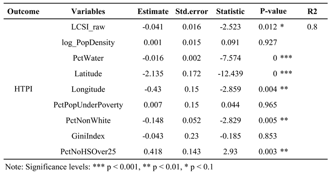
The results show that LCSI was significantly and negatively associated with HTPI (β = -0.041, p = 0.012). This indicates that census tracts with stronger landscape cooling supply tended to experience lower integrated human-relevant thermal pressure after controlling for population density, water proportion, geographic location, socioeconomic characteristics, and county fixed effects. The HTPI model also showed strong overall explanatory performance, with an R² of 0.800.
This finding is important because it extends the evidence from surface-oriented thermal regulation to human-relevant heat-pressure mitigation. While the LSTmax model confirms that LCSI is strongly related to surface thermal condition, the HTPI model shows that landscape cooling supply also has empirical relevance for integrated heat pressure constructed from apparent heat and extreme heat frequency. Therefore, HTPI provides a bridge between the thermal-regulation analysis and the subsequent cooling supply–demand mismatch assessment.

Table 4.
Fixed-effects regression results for integrated human-relevant thermal pressure.
 |
4.3. Explainable GeoAI Analysis of Landscape Effects on Thermal Pressure
4.3.1. Relative Importance of Landscape Components for HTPI
The XGBoost feature-importance results provide an initial ranking of landscape components associated with HTPI (Figure 5). Among all predictors, PctVegeArea showed the highest relative importance, indicating that overall vegetation coverage was the most influential landscape variable in explaining variation in HTPI. This result suggests that broad vegetated land cover, rather than formal park provision alone, plays a central role in shaping human-relevant thermal pressure.
Blue-space and gray-infrastructure variables also ranked highly. PctWater was the second most important predictor, highlighting the relevance of water-area proportion in the landscape cooling process. Road-related and impervious-surface indicators, including RoadDensity, PctImpSurface, and RoadLength_log, also showed substantial importance, suggesting that gray infrastructure contributes meaningfully to the differentiation of thermal pressure across census tracts. In comparison, PctTreeCanopy had a moderate level of importance, while park-related indicators, including PctParkArea, ParkArea_log, and ParkAreaPerCapita_log, ranked lower than vegetation, water, and road-related variables.
The feature-importance ranking indicates that HTPI is more strongly associated with the broader composition of blue–green–gray landscapes than with park provision alone. General vegetation coverage, water-area proportion, and gray-infrastructure intensity appear to be the key landscape dimensions shaping human-relevant thermal pressure. Because XGBoost feature importance provides a relative ranking but does not show the direction or distribution of each variable’s contribution, the following SHAP analysis further examines whether these landscape components increase or decrease predicted HTPI and whether their effects are nonlinear.
4.3.2. SHAP-Based Importance and Directional Effects of Landscape Components
Unlike the XGBoost feature-importance ranking, which only indicates the relative contribution magnitude of each variable, the SHAP analysis identifies both the relative importance and directional contribution of landscape components to HTPI. As shown in Figure 6(a), PctVegeArea had the largest mean absolute SHAP value, indicating that overall vegetation coverage was the most influential landscape variable associated with HTPI. Road-related variables, including RoadLength_log and RoadDensity, and blue-space coverage measured by PctWater also ranked highly. In comparison, PctTreeCanopy showed a moderate contribution, while park-related indicators, including PctParkArea, ParkAreaPerCapita_log, and ParkArea_log, had smaller average SHAP contributions.
Figure 6 (b) provides a more detailed interpretation of how each landscape component contributes to predicted HTPI. SHAP values show both the direction and distribution of variable effects. Positive SHAP values indicate that a variable increases predicted HTPI, whereas negative SHAP values indicate that it decreases predicted HTPI. The color gradient represents the value of each predictor, with red indicating higher values and blue indicating lower values.
The clearest directional pattern is observed for PctVegeArea: high values of PctVegeArea are concentrated on the negative side of the SHAP axis, while low values are mostly located on the positive side. This indicates that census tracts with higher vegetation coverage tend to have lower predicted HTPI, whereas tracts with lower vegetation coverage tend to experience higher predicted human-relevant thermal pressure. The wide SHAP range of PctVegeArea also shows that vegetation coverage has the strongest and most heterogeneous contribution among all landscape predictors. This finding reinforces the interpretation that broad vegetated land cover is the dominant cooling-supportive landscape component in the model.
Blue-space coverage shows a similar cooling-related contribution. Higher values of PctWater are primarily associated with negative SHAP values, suggesting that census tracts with larger water-area proportions tend to have lower predicted HTPI. This pattern is consistent with the expected cooling role of blue spaces in moderating thermal pressure. In contrast, road-related gray infrastructure displays a more heat-amplifying pattern. Higher values of RoadLength_log are more frequently located on the positive side of the SHAP axis, indicating that greater road infrastructure tends to increase predicted HTPI. RoadDensity shows a more dispersed pattern, with both positive and negative SHAP values, suggesting a nonlinear or context-dependent association between road-network intensity and human-relevant thermal pressure.
The contribution of PctTreeCanopy is more moderate than that of overall vegetation coverage. Although tree canopy is generally expected to support cooling through shading and evapotranspiration, its SHAP values are more tightly clustered around zero compared with PctVegeArea. This suggests that tree canopy contributes to variation in predicted HTPI, but its effect is less dominant than the broader vegetation-coverage indicator in this landscape-only model. One possible interpretation is that HTPI, which integrates apparent heat pressure and extreme hot-day frequency, may respond more strongly to broad vegetated land-cover conditions than to canopy coverage alone at the census-tract scale.
Park-related variables show comparatively weaker and more limited directional effects. PctParkArea, ParkArea_log, and ParkAreaPerCapita_log are mostly clustered near zero, indicating that formal park provision has a smaller direct contribution to predicted HTPI than vegetation, water, and road-related variables. This pattern supports the distinction between formal green-space provision and realized cooling function. Parks may provide important recreational and accessibility benefits, but park boundaries alone do not necessarily capture the vegetation structure, tree canopy, water elements, or surface composition that drive cooling-pressure mitigation.
In sum, both XGBoost and SHAP methods consistently identified PctVegeArea as the dominant landscape predictor and highlighted the importance of blue-space and gray-infrastructure variables.
4.4. Cooling Supply–Demand Mismatch
4.4.1. Supply-Demand Mismatch Continuous Map and Quadrant Typology
This study first examined the continuous spatial overlay of landscape cooling supply and heat-sensitive cooling demand (Figure 7) . In this map, the background choropleth represents the normalized Landscape Cooling Supply Index (LCSI_0_1), with darker green indicating higher cooling supply. The graduated red points represent the normalized Heat-sensitive Cooling Demand Index (HCDI_0_1), where larger and darker points indicate stronger heat-sensitive cooling demand. This overlay allows the spatial relationship between cooling supply and demand to be visually assessed before applying the median-based mismatch typology.
The map shows that high heat-sensitive cooling demand is spatially clustered rather than evenly distributed across Maryland census tracts. The most visible clusters of high HCDI occur in the Baltimore metropolitan area, especially Baltimore City and surrounding parts of Baltimore County. A second major concentration appears along the Washington metropolitan corridor, including parts of Prince George’s County and Montgomery County. Additional high-demand points are scattered in Anne Arundel, Harford, Frederick, Washington, and several Eastern Shore counties, although these areas show more dispersed patterns than the Baltimore–Washington corridor.
The spatial overlay also suggests that high cooling demand does not always coincide with high landscape cooling supply. Some high-demand census tracts are located within or adjacent to lighter green areas, indicating relatively lower LCSI values. These areas represent potential cooling-service stress, where heat-sensitive demand is elevated but landscape cooling supply appears insufficient. This pattern is particularly visible in dense urbanized portions of the Baltimore–Washington corridor, where concentrated demand overlaps with fragmented or weaker landscape cooling supply.
At the same time, the map also shows areas where high LCSI values coexist with lower or more dispersed HCDI values. These tracts can be interpreted as relatively buffered areas in which landscape cooling supply is stronger and heat-sensitive demand is less concentrated. In contrast, areas with both darker green backgrounds and high-demand red points indicate high supply–high demand contexts, where existing cooling resources may partially buffer elevated demand but do not eliminate the need for targeted adaptation planning.
This continuous overlay provides the spatial basis for the subsequent four-quadrant mismatch classification. By cross-classifying LCSI and HCDI into high and low groups using median thresholds, the analysis further identifies census tracts that fall into the low supply–high demand category (Figure 8). High supply–low demand tracts represent relatively buffered areas where landscape cooling supply is comparatively strong and heat-sensitive demand is comparatively low. High supply–high demand tracts represent buffered high-demand areas, where elevated heat-sensitive demand overlaps with relatively strong landscape cooling supply. Low supply–low demand tracts represent areas with weaker cooling supply but lower immediate demand pressure. Low supply–high demand tracts were defined as priority mismatch areas because they combine insufficient landscape cooling supply with elevated heat-sensitive cooling demand.
The four-quadrant classification identified 433 census tracts, accounting for 31.3% of all Maryland census tracts, as low supply–high demand priority mismatch areas. The same number of tracts were classified as high supply–low demand areas, while high supply–high demand and low supply–low demand areas accounted for 18.8% and 18.7% of tracts, respectively. This distribution indicates that cooling supply and heat-sensitive demand are not evenly aligned across Maryland.
4.4.2. Spatial Concentration of Low Supply–High Demand Priority Mismatch Tracts
Figure 9 further examines the spatial distribution of low supply–high demand priority mismatch tracts in relation to population density. The black-outlined census tracts represent areas classified as low landscape cooling supply and high heat-sensitive cooling demand, while the background choropleth shows population density measured as persons per square mile. This overlay helps distinguish priority mismatch areas located in densely populated urban corridors from those located in sparsely populated rural or coastal contexts.
The map shows that priority mismatch tracts are not randomly distributed across Maryland. A prominent concentration appears in the Baltimore metropolitan area, especially Baltimore City and adjacent portions of Baltimore County. Many of these tracts are located in areas with high population density, indicating that landscape cooling deficits and heat-sensitive demand coincide with large exposed populations. A second important concentration appears along the Washington metropolitan corridor, particularly in parts of Prince George’s County and Montgomery County. These areas are especially important from an implementation perspective because they combine low cooling supply, high heat-sensitive demand, and high population density.
Priority mismatch tracts also appear in parts of Howard, Anne Arundel, Harford, Frederick, and Washington counties, suggesting that cooling-service deficits extend beyond the two largest urban cores. In these areas, priority mismatch tracts are often located near suburban growth zones, transportation corridors, or urbanizing edges, where gray infrastructure and fragmented cooling landscapes may overlap with socially vulnerable or heat-sensitive populations. This pattern indicates that mismatch is not only an inner-city issue but also occurs in suburban and peri-urban contexts.
A more dispersed pattern is observed in the Eastern Shore and southeastern parts of Maryland, including parts of Wicomico, Worcester, Somerset, Dorchester, Talbot, Caroline, and nearby counties. Some of these priority mismatch tracts are located in areas with relatively low population density. This does not necessarily mean that they should be interpreted as the highest implementation priority in terms of the number of residents affected. Rather, these tracts indicate high relative demand intensity under the current HCDI construction, which is based on standardized thermal pressure and socio-demographic sensitivity indicators rather than population-weighted exposure.
The population-density overlay therefore refines the interpretation of the mismatch typology. The low supply–high demand category identifies census tracts where cooling-service deficits and heat-sensitive demand intensity overlap, while population density helps identify where such mismatch may affect larger numbers of residents. From a planning perspective, the Baltimore–Washington corridor represents the most practically significant concentration of priority mismatch because low cooling supply, high heat-sensitive demand, and dense population settlement occur together.
5. Discussion
LCSI is not merely a categorical urban–rural contrast, but a continuous tract-level measure of cooling supply heterogeneity. This finding supports the need to evaluate cooling supply at the census-tract scale rather than relying only on county-level or broad regional classifications. The observed spatial heterogeneity also provides the empirical basis for the subsequent analysis, which tests whether higher LCSI is associated with realized thermal regulation and whether low-supply areas overlap with high heat-sensitive cooling demand.
The SHAP beeswarm results show that human-relevant thermal pressure is shaped more strongly by broad blue–green–gray landscape composition than by park provision alone. Higher vegetation coverage and water-area proportion tend to reduce predicted HTPI, whereas road-related gray infrastructure tends to increase or nonlinearly shape thermal pressure. These findings support the need to distinguish vegetation-based cooling function from formal green-space provision when evaluating landscape cooling services.
A notable finding is that some low supply–high demand tracts are located in relatively low-density rural or coastal areas, especially in southeastern Maryland and the Eastern Shore. This does not necessarily indicate a model problem. Rather, it reflects that the demand index used in this study measures relative heat-sensitive demand intensity, not the absolute number of people exposed. A sparsely populated tract can still be identified as high demand if it has a higher proportion of older residents, more socially isolated older households, weaker access to household cooling, greater socioeconomic disadvantage, or stronger heat pressure.
This distinction is important for interpreting priority mismatch areas. Low supply–high demand tracts in rural or coastal areas represent localized vulnerability pockets, where a small population may still face substantial heat-related constraints. In contrast, low supply–high demand tracts in the Baltimore–Washington corridor have stronger implementation significance because cooling deficits, heat-sensitive demand, and high population density overlap. These areas are more likely to generate larger public benefits from landscape-based cooling interventions, such as tree-canopy expansion, neighborhood greening, and gray-surface retrofitting.
Therefore, the mismatch results should be interpreted in two layers. The first layer identifies where relative cooling demand intensity exceeds local landscape cooling supply. The second layer considers population concentration to distinguish where interventions may benefit larger numbers of residents. This interpretation avoids overlooking rural vulnerability while still recognizing the practical priority of densely populated urban corridors. Future studies could further develop population-weighted mismatch indicators, incorporate finer residential population data, and test whether priority areas remain stable under alternative thresholds and index-weighting schemes.
6. Conclusions
This study developed a cooling-service cascade framework to examine how blue–green–gray landscape composition shapes landscape cooling supply, realized thermal regulation, human-relevant thermal pressure, and supply–demand mismatch across 1,385 census tracts in Maryland. The results show that landscape cooling supply is spatially uneven rather than uniformly distributed across urban, suburban, coastal, and rural contexts. The constructed Landscape Cooling Supply Index reveals a clear tract-level gradient, with stronger cooling supply generally associated with higher vegetation coverage, tree canopy, park provision, water-area proportion, and weaker gray-infrastructure pressure. This pattern confirms that landscape cooling capacity cannot be reduced to the presence of green space alone; it is produced by the combined structure of blue, green, and gray landscape components.
The regression results further demonstrate that higher landscape cooling supply is associated with lower thermal pressure, although this relationship varies across thermal indicators. The association is strongest for surface thermal conditions, remains significant for apparent heat pressure, and is also evident for the integrated Human-Relevant Thermal Pressure Index. This finding is important because it suggests that landscape cooling supply is not only linked to land surface temperature reduction, but also to heat conditions more directly relevant to human exposure. At the same time, the weak correspondence between surface temperature and human-relevant thermal indicators indicates that surface cooling should not be treated as a complete proxy for heat adaptation performance. A landscape may reduce surface heat while still failing to sufficiently reduce human-experienced thermal pressure.
The explainable GeoAI analysis provides a more detailed interpretation of the landscape processes underlying this relationship. Both XGBoost feature importance and SHAP-based interpretation consistently identify overall vegetation coverage as the most influential landscape component associated with human-relevant thermal pressure. Water-area proportion and road-related gray infrastructure also play important roles, while formal park provision shows weaker direct contributions. The SHAP results further reveal that high vegetation coverage and water-area proportion tend to reduce predicted thermal pressure, whereas road infrastructure tends to increase or nonlinearly shape it. These findings suggest that effective cooling-service planning should move beyond park quantity or green-space designation and pay closer attention to vegetation structure, blue-space presence, and the thermal burden created by gray infrastructure.
The supply–demand mismatch analysis translates these findings into a planning-relevant spatial diagnosis. A total of 433 census tracts, accounting for 31.3% of all Maryland census tracts, were classified as low supply–high demand priority mismatch areas. These tracts include both densely populated areas in the Baltimore–Washington corridor and more dispersed rural or coastal vulnerability pockets. This distinction shows that cooling mismatch has two meanings: in dense urban corridors, it indicates places where interventions may benefit larger exposed populations; in low-density areas, it identifies localized vulnerability where small populations may still face substantial heat-related constraints. By connecting landscape composition, thermal regulation, human-relevant pressure, and demand-sensitive mismatch, this study provides a framework for identifying where landscape-based cooling interventions are most needed and how urban climate adaptation can become more spatially targeted, socially sensitive, and ecologically grounded.
References
- Anderson, G. B.; Bell, M. L.; Peng, R. D. Methods to calculate the heat index as an exposure metric in environmental health research. Environ. Health Perspect. 2013, 121(10), 1111–1119. [Google Scholar] [CrossRef] [PubMed]
- Anguelovski, I.; Connolly, J. J. T.; Brand, A. L. From landscapes of utopia to the margins of the green urban life: For whom is the new green city? City 2018, 22(3), 417–436. [Google Scholar] [CrossRef]
- Athokpam, V.; Chamroy, T.; Ngairangbam, H. The role of urban green spaces in mitigating climate change: An integrative review of ecological, social, and health benefits. Environ. Rep. An. Int. J. 2024, 10–14. [Google Scholar] [CrossRef]
- Benedict, M. A.; McMahon, E. T. Green Infrastructure: Linking Landscapes and Communities; Island Press, 2006. [Google Scholar]
- Benz, S. A.; Burney, J. A. Widespread race and class disparities in surface urban heat extremes across the United States. Earth's Future 2021, 9(7), e2021EF002016. [Google Scholar] [CrossRef]
- Bowler, D. E.; Buyung-Ali, L.; Knight, T. M.; Pullin, A. S. Urban greening to cool towns and cities: A systematic review of the empirical evidence. Landsc. Urban Plan. 2010, 97(3), 147–155. [Google Scholar] [CrossRef]
- Burkhard, B.; Kroll, F.; Nedkov, S.; Müller, F. Mapping ecosystem service supply, demand and budgets. Ecol. Indic. 2012, 21, 17–29. [Google Scholar] [CrossRef]
- Butt, A. N.; Rigoni, C. The Green Blueprint: Designing Future Cities with Urban Green Infrastructure and Ecosystem Services in the UK. Land 2025, 14(6), 1306. [Google Scholar] [CrossRef]
- Campbell, A.; Chanse, V.; Schindler, M. Developing a conceptual framework for characterizing and measuring social resilience in blue-green infrastructure (BGI). SUSTAINABILITY 2024, 16(9), 3847. [Google Scholar] [CrossRef]
- Chakraborty, T.; Hsu, A.; Manya, D.; Sheriff, G. Disproportionately higher exposure to urban heat in lower-income neighborhoods: A multi-city perspective. Environ. Res. Lett. 2019, 14(10), 105003. [Google Scholar] [CrossRef]
- Chen, H.; Zhao, L.; Dong, W.; Cheng, L.; Cai, W.; Yang, J.; Bao, J.; Liang, X. Z.; Hajat, S.; Gong, P.; Liang, W.; Huang, C. Spatiotemporal Variation of Mortality Burden Attributable to Heatwaves in China, 1979-2020. Sci. Bull. 2022, 67(13), 1340–1344. [Google Scholar] [CrossRef] [PubMed]
- Geijzendorffer, I. R.; Martín-López, B.; Roche, P. K. Improving the identification of mismatches in ecosystem services assessments. Ecol. Indic. 2015, 52, 320–331. [Google Scholar] [CrossRef]
- Guardaro, M.; Hondula, D. M.; Ortiz, J.; Redman, C. L. Adaptive capacity to extreme urban heat: The dynamics of differing narratives. Clim. Risk Manag. 2022, 35, 100415. [Google Scholar] [CrossRef]
- Haines-Young, R.; Potschin, M. The Links between Biodiversity, Ecosystem Services and Human Well-Being. Ecosyst. Ecol. A New Synth. 2010, 1, 110–139. [Google Scholar] [CrossRef]
- Herath, P.; Bai, X. Benefits and co-benefits of urban green infrastructure for sustainable cities: six current and emerging themes. Sustain. Sci. 2024, 19(3), 1039–1063. [Google Scholar] [CrossRef]
- Harlan, S. L.; Ruddell, D. M. Climate change and health in cities: Impacts of heat and air pollution and potential co-benefits from mitigation and adaptation. Curr. Opin. Environ. Sustain. 2011, 3(3), 126–134. [Google Scholar] [CrossRef]
- Hsu, A.; Sheriff, G.; Chakraborty, T.; Manya, D. Disproportionate exposure to urban heat island intensity across major US cities. Nat. Commun. 2021, 12(1), 2721. [Google Scholar] [CrossRef] [PubMed]
- Jabbar, H. K.; Hamoodi, M. N.; Al-Hameedawi, A. N. Urban heat islands: a review of contributing factors, effects and data. In IOP Conference Series: Earth and Environmental Science; IOP Publishing, January 2023; Vol. 1129, No. 1, p. 012038. [Google Scholar]
- Jennings, V.; Johnson Gaither, C. Approaching environmental health disparities and green spaces: An ecosystem services perspective. Int. J. Environ. Res. Public Health 2015, 12(2), 1952–1968. [Google Scholar] [CrossRef] [PubMed]
- Jesdale, B. M.; Morello-Frosch, R.; Cushing, L. The Racial/Ethnic Distribution of Heat Risk-Related Land Cover in Relation to Residential Segregation [Article]. Environ. Health Perspect. 2013, 121(7), 811–817. [Google Scholar] [CrossRef] [PubMed]
- Kabisch, N.; Qureshi, S.; Haase, D. Human-environment interactions in urban green spaces: A systematic review of contemporary issues and prospects for future research. Environ. Impact Assess. Rev. 2015, 50, 25–34. [Google Scholar] [CrossRef]
- Karimi, A.; Mohammad, P.; Garcia-Martinez, A.; Moreno-Rangel, D.; Gachkar, D.; Gachkar, S. New developments and future challenges in reducing and controlling heat island effect in urban areas. Environ. Dev. Sustain. 2023, 25(10), 10485–10531. [Google Scholar]
- Kim, D.; Song, S. K. The multifunctional benefits of green infrastructure in community development: An analytical review based on 447 cases. Sustainability 2019, 11(14), 3917. [Google Scholar] [CrossRef] [PubMed]
- Kim, Y.-o.; Lee, W.; Kim, H.; Cho, Y. Social isolation and vulnerability to heatwave-related mortality in the urban elderly population: A time-series multi-community study in Korea. Environ. Int. 2020, 142, 105868. [Google Scholar] [CrossRef] [PubMed]
- Kovats, R. S.; Hajat, S. Heat Stress and Public Health: A Critical Review. Annu. Rev. Public Health 2008, 29, 41–55. [Google Scholar] [CrossRef] [PubMed]
- Li, Y.; Ren, C.; Ho, J. Y.-e.; Shi, Y. Landscape metrics in assessing how the configuration of urban green spaces affects their cooling effect: A systematic review of empirical studies. Landsc. Urban Plan. 2023, 239, 104842. [Google Scholar] [CrossRef]
- Li, Y.; Svenning, J.-C.; Zhou, W.; Zhu, K.; Abrams, J. F.; Lenton, T. M.; Ripple, W. J.; Yu, Z.; Teng, S. N.; Dunn, R. R. Green spaces provide substantial but unequal urban cooling globally. Nat. Commun. 2024, 15(1), 7108. [Google Scholar] [CrossRef] [PubMed]
- Liu, P.; Lei, C.; Wang, H.; Zhang, J.; Xia, S.; Cao, J. Driving Mechanisms of Blue–Green Infrastructure in Enhancing Urban Sustainability: A Spatial–Temporal Assessment from Zhenjiang, China. Land 2026, 15(2), 233. [Google Scholar] [CrossRef]
- Marketaki, A.; Tseliou, A.; Tousi, E.; Mela, A.; Zervas, E. Urban Green Network Design as an Adaptation Strategy of Mediterranean Cities to Rising Temperatures. Land 2026, 15(6), 908. [Google Scholar] [CrossRef]
- Meerow, S.; Newell, J. P. Spatial planning for multifunctional green infrastructure: Growing resilience in Detroit. Landsc. Urban Plan. 2017, 159, 62–75. [Google Scholar] [CrossRef]
- Norton, B. A.; Coutts, A. M.; Livesley, S. J.; Harris, R. J.; Hunter, A. M.; Williams, N. S. Planning for Cooler Cities: A Framework to Prioritise Green Infrastructure to Mitigate High Temperatures in Urban Landscapes. Landsc. Urban Plan. 2015, 134, 127–138. [Google Scholar] [CrossRef]
- Oke, T. R. The Energetic Basis of the Urban Heat-Island [Article]. Q. J. R. Meteorol. Soc. 1982, 108(455), 1–24. [Google Scholar] [CrossRef]
- Peng, B.; Hendricks, M. D.; Hancock, G. R. Reexploring the conception of heat–health risk: From the perspectives of dimensionality and spatiality. Risk Anal. 2025, 45(5), 1132–1151. [Google Scholar] [PubMed]
- Perkins, S. E. A review on the scientific understanding of heatwaves—Their measurement, driving mechanisms, and changes at the global scale. Atmos. Res. 2015, 164-165, 242–267. [Google Scholar] [CrossRef]
- Rahimi, E.; Barghjelveh, S.; Dong, P. Quantifying how urban landscape heterogeneity affects land surface temperature at multiple scales. J. Ecol. Environ. 2021, 45, 22. [Google Scholar] [CrossRef]
- Rothfusz, L. P. The heat index equation (or, more than you ever wanted to know about heat index) [NWS Southern Region Technical Attachment SR 90-23]. 1990. Available online: https://www.weather.gov/media/ffc/ta_htindx.PDF.
- Siehr, S. A.; Sun, M.; Aranda Nucamendi, J. L. Blue-green infrastructure for climate resilience and urban multifunctionality in Chinese cities. Wiley Interdiscip. Rev. Energy Environ. 2022, 11(5), e447. [Google Scholar] [CrossRef]
- Syrbe, R.-U.; Meier, S.; Moyzes, M.; Dworczyk, C.; Grunewald, K. Assessment and monitoring of local climate regulation in cities by green infrastructure—A national ecosystem service indicator for Germany. Land 2024, 13(5), 689. [Google Scholar] [CrossRef]
- Turner, M. G. Landscape ecology: The effect of pattern on process. Annu. Rev. Ecol. Syst. 1989, 20, 171–197. [Google Scholar] [CrossRef]
- Turner, V. K.; Rogers, M. L.; Zhang, Y.; Middel, A.; Schneider, F. A.; Ocón, J. P.; Seeley, M.; Dialesandro, J. J. More than surface temperature: Mitigating thermal exposure in hyper-local land system. J. Land Use Sci. 2022, 17(1), 79–99. [Google Scholar] [CrossRef]
- Tzoulas, K.; Korpela, K.; Venn, S.; Yli-Pelkonen, V.; Kaźmierczak, A.; Niemela, J.; James, P. Promoting ecosystem and human health in urban areas using green infrastructure: A literature review. Landsc. Urban Plan. 2007, 81(3), 167–178. [Google Scholar] [CrossRef]
- Venter, Z. S.; Krog, N. H.; Barton, D. N. Linking Green Infrastructure to Urban Heat and Human Health Risk Mitigation in Oslo, Norway [Article]. Sci. Total Environ. 2020, 709, 136193, Article 136193. [Google Scholar] [CrossRef] [PubMed]
- Villamagna, A. M.; Angermeier, P. L.; Bennett, E. M. Capacity, pressure, demand, and flow: A conceptual framework for analyzing ecosystem service provision and delivery. Ecol. Complex. 2013, 15, 114–121. [Google Scholar] [CrossRef]
- Voogt, J. A.; Oke, T. R. Thermal Remote Sensing of Urban Climates [Review]. Remote Sens. Environ. 2003, 86(3), 370–384. [Google Scholar] [CrossRef]
- Wang, S.; Chen, H.; Guo, Y. l.; Su, W.; Xu, Y.; Cui, S.; Zhou, Z. Interpretation of spatial and temporal changes and drivers of ecological source regions based on LightGBM-SHAP. AIP Adv. 2024, 14(6). [Google Scholar] [CrossRef]
- Weng, Q. H. Thermal Infrared Remote Sensing for Urban Climate and Environmental Studies: Methods, Applications, and Trends [Review]. ISPRS J. Photogramm. Remote Sens. 2009, 64(4), 335–344. [Google Scholar] [CrossRef]
- Wolch, J. R.; Byrne, J.; Newell, J. P. Urban Green Space, Public Health, and Environmental Justice: The Challenge of Making Cities ‘Just Green Enough’. In Landscape and Urban Planning; 2014; Volume 125 SRC - BaiduScholar, pp. 234–244. [Google Scholar]
- Wolff, S.; Schulp, C. J. E.; Verburg, P. H. Mapping ecosystem services demand: A review of current research and future perspectives. Ecol. Indic. 2015, 55, 159–171. [Google Scholar] [CrossRef]
- Zhou, W. Q.; Huang, G. L.; Cadenasso, M. L. Does Spatial Configuration Matter? Understanding the Effects of Land Cover Pattern on Land Surface Temperature in Urban Landscapes [Article]. Landsc. Urban Plan. 2011, 102(1), 54–63. [Google Scholar] [CrossRef]
- Zhou, X.; Wang, Y.-C. Spatial–Temporal Dynamics of Urban Green Space in Response to Rapid Urbanization and Greening Policies. Landsc. Urban Plan. 2011, 100(3), 268–277. [Google Scholar] [CrossRef]
- Ziter, C. D.; Pedersen, E. J.; Kucharik, C. J.; Turner, M. G. Scale-Dependent Interactions between Tree Canopy Cover and Impervious Surfaces Reduce Daytime Urban Heat During Summer. Proc. Natl. Acad. Sci. 2019, 116(15), 7575–7580. [Google Scholar] [CrossRef] [PubMed]
Figure 1.
Study Area: State of Maryland.
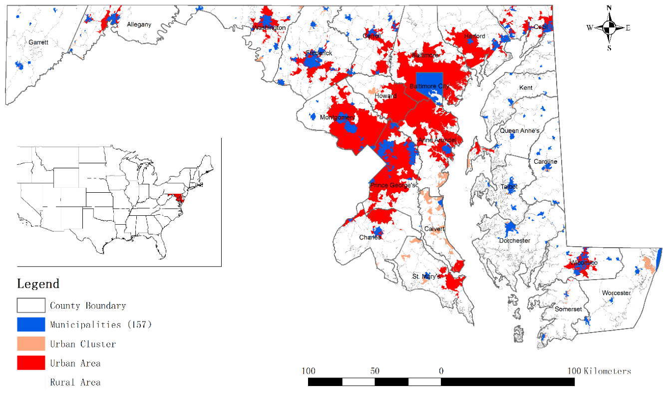
Figure 2.
A Green-Space Cooling-Service Cascade Framework
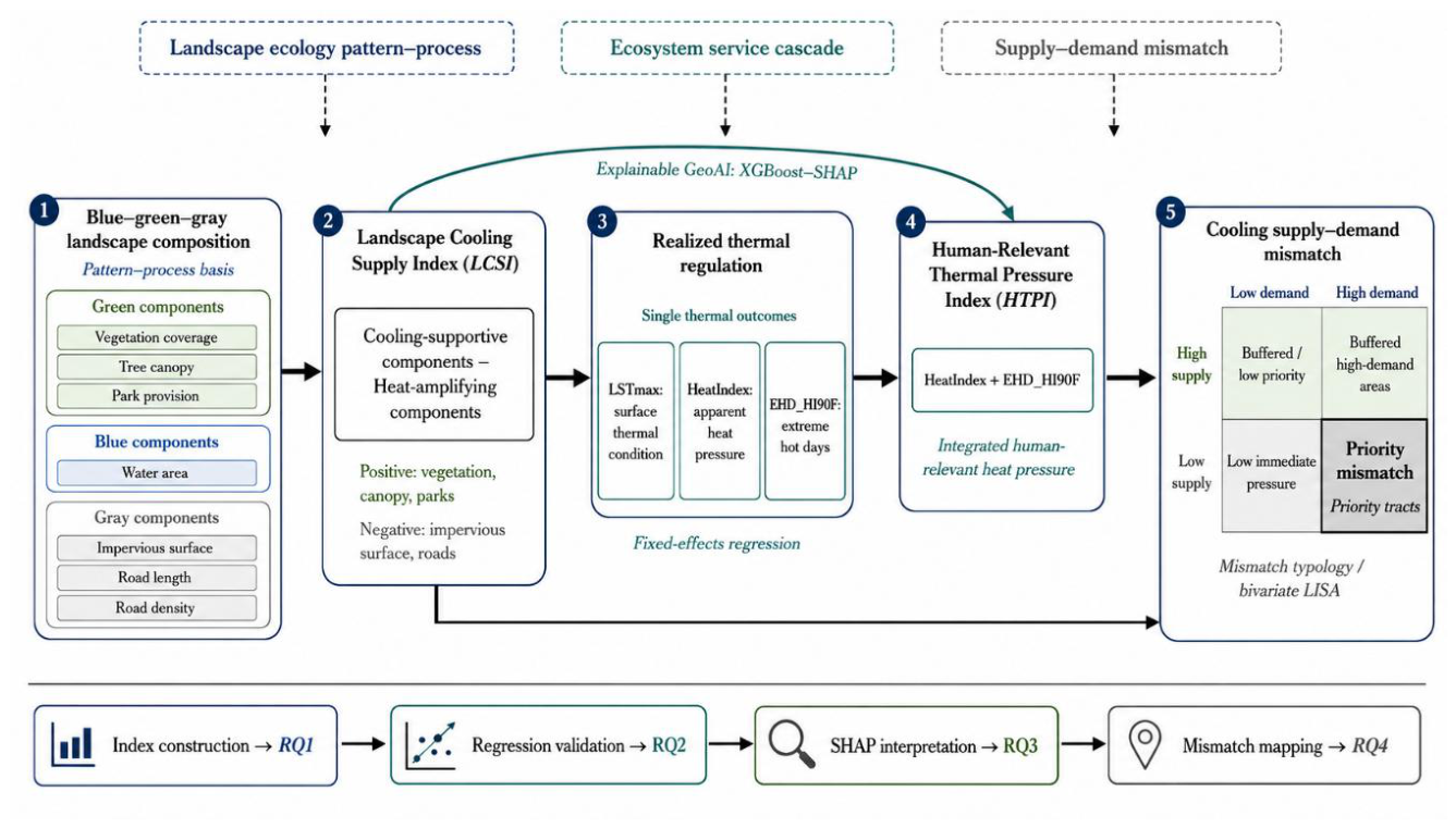
Figure 3.
LCSI (Density) Distribution and Descriptive Statistics.
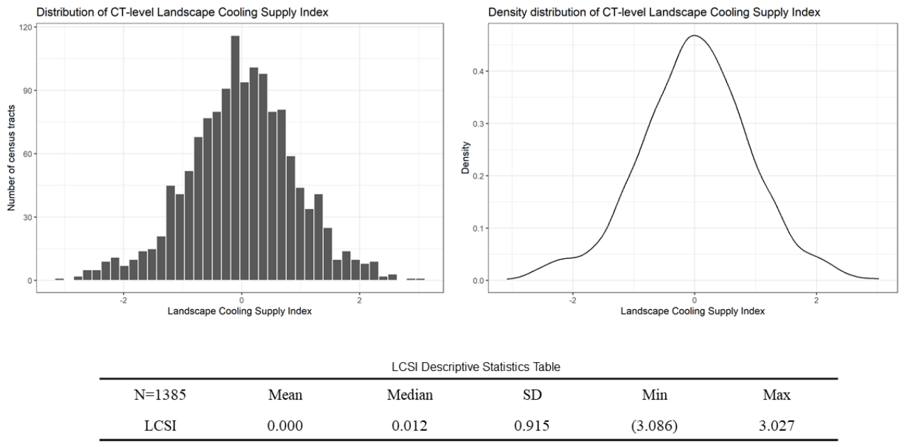
Figure 4.
Spatial distribution of the Landscape Cooling Supply Index (LCSI) across Maryland census tracts.
Figure 4.
Spatial distribution of the Landscape Cooling Supply Index (LCSI) across Maryland census tracts.
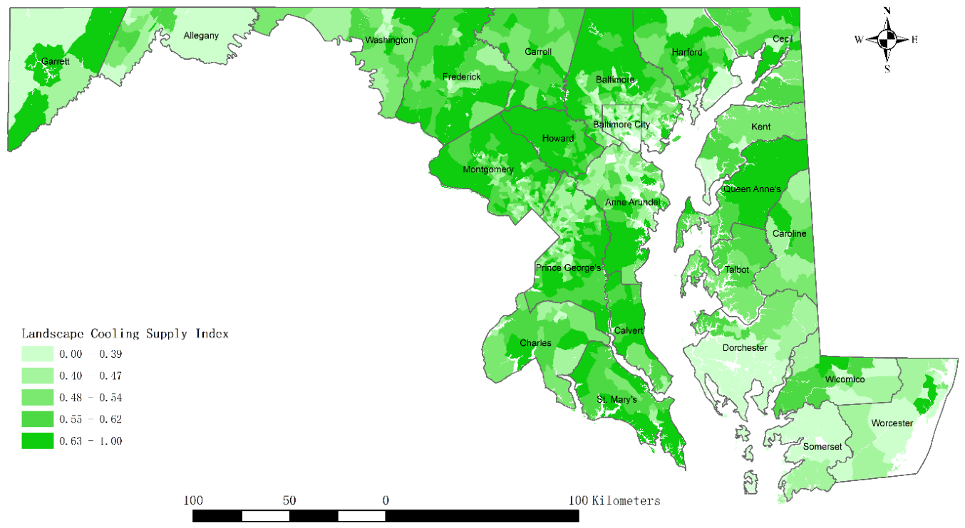
Figure 5.
XGBoost feature importance of landscape components for HTPI. Note: The figure shows the relative importance of landscape predictors in the XGBoost model. Higher values indicate stronger contribution to model splitting and prediction of HTPI.
Figure 5.
XGBoost feature importance of landscape components for HTPI. Note: The figure shows the relative importance of landscape predictors in the XGBoost model. Higher values indicate stronger contribution to model splitting and prediction of HTPI.
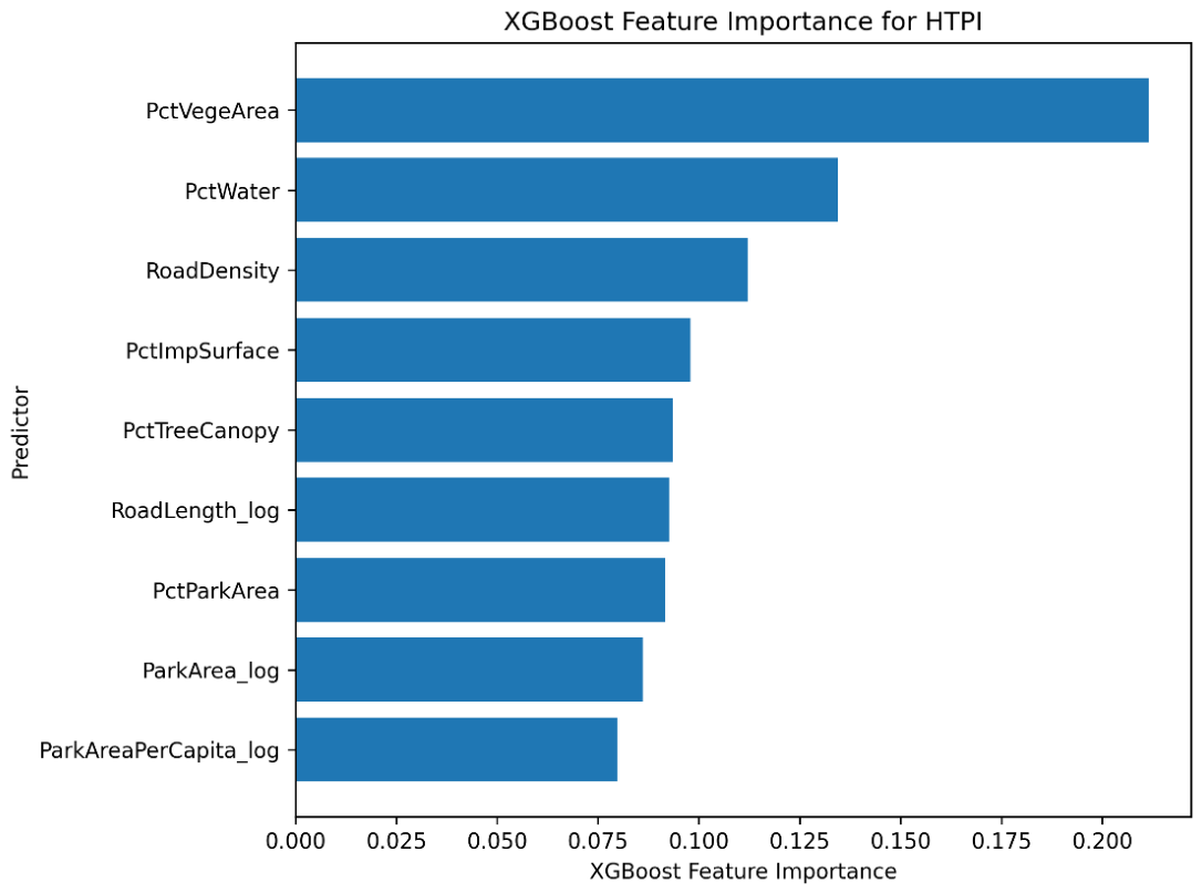
Figure 6.
SHAP-based global importance and directional effects of landscape components on HTPI.
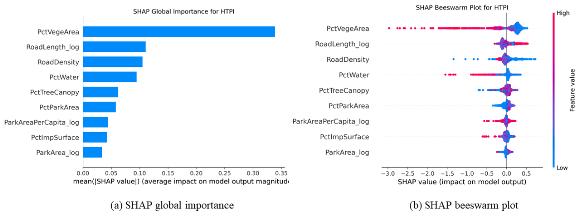
Figure 7.
Spatial Overlay of Landscape Cooling Supply and Heat-sensitive Cooling Demand across Maryland Census Tracts. Note:L The background choropleth shows the normalized Landscape Cooling Supply Index (LCSI_0_1) using five quantile classes. Graduated red points show the normalized Heat-sensitive Cooling Demand Index (HCDI_0_1), with larger and darker points indicating higher heat-sensitive cooling demand.
Figure 7.
Spatial Overlay of Landscape Cooling Supply and Heat-sensitive Cooling Demand across Maryland Census Tracts. Note:L The background choropleth shows the normalized Landscape Cooling Supply Index (LCSI_0_1) using five quantile classes. Graduated red points show the normalized Heat-sensitive Cooling Demand Index (HCDI_0_1), with larger and darker points indicating higher heat-sensitive cooling demand.
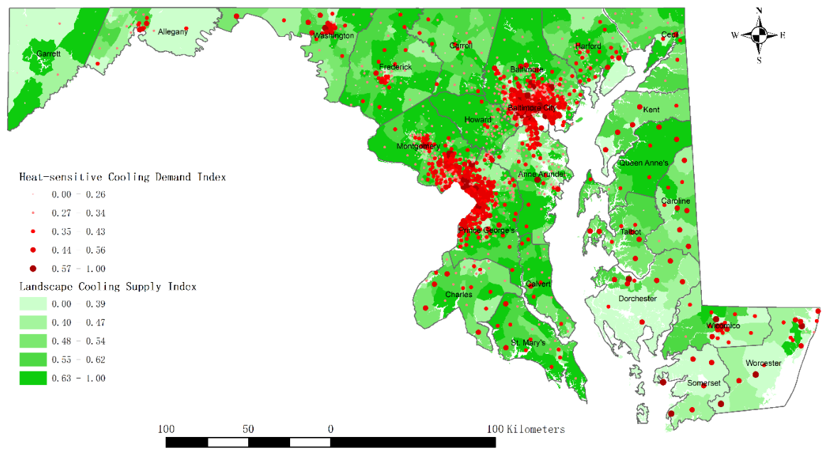
Figure 8.
Four-quadrant Mismatch Typology.
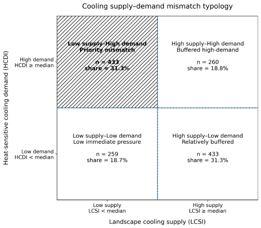
Figure 9.
Spatial Distribution of Priority Mismatch Tracts with Population Density.
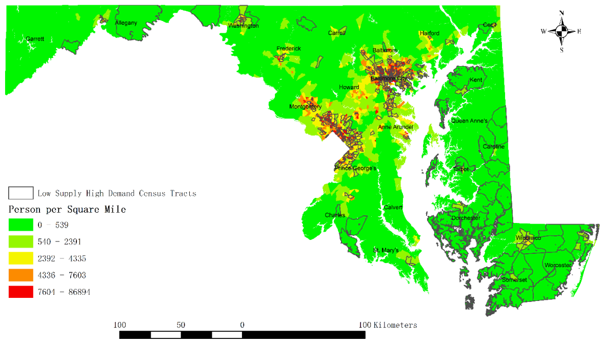
Table 1.
Indicators for green-space cooling supply and heat-amplifying gray infrastructure.
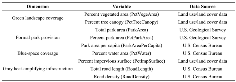 |
Table 2.
Correlations among thermal indicators.
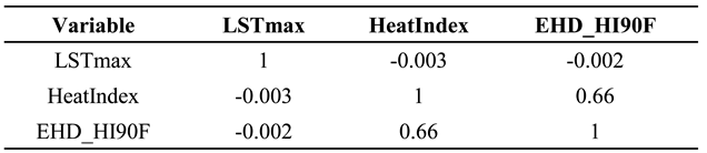 |
Table 3.
Fixed-effects regression results for single thermal outcomes.
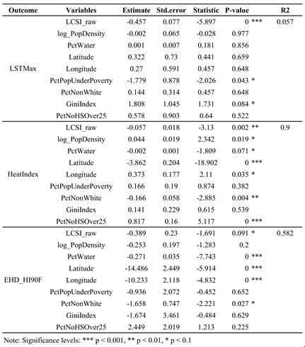 |
Disclaimer/Publisher’s Note: The statements, opinions and data contained in all publications are solely those of the individual author(s) and contributor(s) and not of MDPI and/or the editor(s). MDPI and/or the editor(s) disclaim responsibility for any injury to people or property resulting from any ideas, methods, instructions or products referred to in the content. |
© 2026 by the authors. Licensee MDPI, Basel, Switzerland. This article is an open access article distributed under the terms and conditions of the Creative Commons Attribution (CC BY) license (http://creativecommons.org/licenses/by/4.0/).
Copyright: This open access article is published under a Creative Commons CC BY 4.0 license, which permit the free download, distribution, and reuse, provided that the author and preprint are cited in any reuse.


