Submitted:
22 June 2026
Posted:
23 June 2026
You are already at the latest version
Abstract
This paper presents a hybrid computer vision framework that explicitly decouples geometric stem measurement from visual foliage condition classification for automated post-harvest quality assessment of Ruscus hypophyllum ornamental foliage. The proposed approach addresses a gap in the literature where heterogeneous quality attributes are typically treated within a single unified learning framework. In the first stage, stem size is estimated using a pixel-based geometric method that incorporates trigonometric orientation correction and spatial calibration via a reference marker of known length, enabling accurate conversion of image measurements to real-world physical dimensions. In the second stage, foliage condition is classified as good or poor using supervised machine learning models trained on Bag of Features representations extracted with the SIFT descriptor. A dataset of 1,233 Ruscus hypophyllum images was acquired under controlled conditions using a consumer-grade smartphone camera and processed using open-source Python libraries. Twenty-four classifier configurations across six model families were evaluated using stratified 10-fold cross-validation. The geometric estimation stage achieved a Mean Absolute Error (MAE) of 1.2 mm, a Root Mean Square Error (RMSE) of approximately 1.3 mm, and a size categorization accuracy of 99.84%. For foliage condition classification, the Linear Support Vector Machine achieved the best performance, with an accuracy of 92.4 ± 1.0% and an F1-score of 91.1±1.2%, outperforming all other evaluated configurations. The proposed framework provides an interpretable, computationally efficient, and accessible solution for automated foliage quality grading, with potential applications in export-oriented ornamental foliage processing facilities.
Keywords:
post-harvest quality assessment
; ornamental foliage
; Ruscus hypophyllum
; machine vision
; intelligent inspection
; geometric measurement
; SIFT descriptor
; Support Vector Machine
1. Introduction
Agricultural production and the export of ornamental plants represent an important economic sector in several countries, including Ecuador. The global ornamental horticulture industry—encompassing cut flowers, potted plants, and cut foliage—currently generates more than USD 130 billion annually, involving more than 90 countries worldwide [1]. Within this context, Ecuador has consolidated its position as one of the leading exporters of ornamental plants and cut flowers at the international level, with floriculture constituting one of the most dynamic areas of its national economy in terms of export value and rural employment generation [2]. Among commercially relevant ornamental species, Ruscus hypophyllum has gained increasing importance in international floral markets due to its durability, aesthetic characteristics, and suitability for floral arrangements [3]. The ornamental horticulture sector is highly competitive, driven by continuous advances in infrastructure availability, variety development, and post-harvest handling technologies [4]. In post-harvest processing chains, product quality cannot be improved after harvest but only preserved, making consistent and reliable quality assessment a critical factor for competitiveness in global markets [1].
The post-harvest handling of ornamental foliage typically involves several stages, including harvesting, selection, classification, and packaging. In many production systems, these processes are still carried out manually by trained workers who evaluate visual characteristics such as stem length, leaf distribution, and overall plant condition. However, manual inspection presents well-documented limitations in agricultural quality control contexts: it is inherently subjective, prone to inter-operator variability, and inefficient for large-scale production environments [5,6]. In particular, visual assessments performed by different operators on the same batch of products have been shown to yield inconsistent results, compromising the reliability of quality grading [7]. Furthermore, the physical demands of repetitive manual inspection reduce throughput and increase the risk of error [6]. These limitations are especially critical in export-oriented post-harvest chains, where strict and consistent quality standards must be met to satisfy international market requirements [3]. These limitations motivate the development of automated vision-based inspection systems capable of providing objective, repeatable, and scalable quality assessments in post-harvest processing environments.
Recent advances in computer vision and machine learning have enabled the development of automated inspection systems across a wide range of agricultural applications, including fruit grading, plant disease detection, and crop monitoring [6,8,9,10]. These systems typically rely on image-based feature extraction combined with supervised learning models to classify agricultural products according to predefined quality criteria [5,7].
Within the specific domain of ornamental plant inspection, computer vision techniques have been applied to the classification and grading of cut flowers. A hybrid vision-based approach for the identification of Anthurium flower cultivars was proposed in [11], combining geometric feature extraction with machine learning classifiers and achieving classification accuracies above 99%. More recently, image-based deep learning methods have been explored for quality grading of cut flowers based on maturity status, demonstrating the feasibility of automated ornamental grading under controlled acquisition conditions [12]. Automated trait estimation in ornamental floriculture has also been investigated using convolutional neural networks, yielding accuracies between 35% and 99% depending on the trait evaluated [13]. However, these studies focus primarily on flower-type ornamentals and do not address the specific challenges associated with cut foliage species such as Ruscus hypophyllum, where both stem morphology and foliar condition must be jointly assessed.
Regarding the geometric measurement of plant traits, image-based methods have been successfully applied to non-destructive estimation of morphological parameters such as stem length, plant height, and leaf area [14,15]. These approaches typically rely on spatial calibration using reference markers and scale factors to convert pixel measurements into real-world dimensions, as reviewed in the context of precision agriculture and plant phenotyping [16,17]. Despite their demonstrated effectiveness, such geometric methods have not been systematically combined with visual quality classification for post-harvest foliage assessment, representing a gap that the present work seeks to address.
Table 1 summarizes representative studies on vision-based quality assessment of ornamental plants, highlighting the species, attributes evaluated, methodological approach, and reported accuracy. As shown, existing work focuses primarily on flower-type ornamentals and does not simultaneously address geometric and visual quality attributes in cut foliage species such as Ruscus hypophyllum.
Classical machine learning models—including Support Vector Machines, Decision Trees, Naive Bayes, and k-Nearest Neighbors—remain competitive and widely used in image classification tasks that involve structured feature representations under limited data conditions [19,20]. In particular, the Bag of Features framework combined with local descriptors such as SIFT has demonstrated robust performance in plant-related classification tasks where deep learning approaches may be constrained by dataset size [21,22]. These characteristics make classical models particularly suitable for the controlled acquisition scenario addressed in this work.
Despite these advances, most existing approaches treat quality assessment as a unified classification task, in which all attributes of interest are learned simultaneously by the model [8,11]. In the case of ornamental foliage such as Ruscus hypophyllum, however, quality assessment involves two fundamentally different types of attributes: measurable physical properties—such as stem length—that can be precisely estimated using geometric image analysis, and visual attributes—such as leaf density, color uniformity, and foliar damage—that require learning-based classification. Treating these heterogeneous attributes within a single unified framework introduces unnecessary complexity in three specific dimensions: it increases the amount of labeled training data required to jointly learn geometric and visual patterns, reduces model interpretability by conflating deterministic and statistical processes within a single learned representation, and obscures the availability of deterministic geometric methods that are both more accurate and more transparent than learned models for measurable physical traits [15,18].
To address this gap, this paper proposes a two-stage hybrid computer vision framework for the automated quality assessment of Ruscus hypophyllum foliage. In the first stage, stem size is estimated using a geometric pixel-based method that incorporates trigonometric orientation correction and spatial calibration via a reference marker, enabling accurate conversion of image measurements to real-world dimensions [16,17]. In the second stage, foliage condition is classified as good or poor using supervised machine learning models trained on Bag of Features representations extracted with the SIFT descriptor [23,24]. By decoupling these two tasks, the proposed system achieves both high measurement accuracy and interpretable quality classification without requiring a unified end-to-end learning model.
The main contributions of this work are as follows:
- A hybrid two-stage framework that explicitly decouples geometric stem measurement from visual foliage condition classification, improving system interpretability and reducing model complexity compared to unified classification approaches.
- A pixel-based stem size estimation method incorporating trigonometric orientation correction and reference-marker spatial calibration, enabling accurate conversion of pixel measurements to real-world physical dimensions under controlled acquisition conditions.
- A systematic comparative evaluation of classical supervised machine learning classifiers on Bag of Features representations, providing evidence-based guidance on model selection for structured visual feature spaces in agricultural inspection tasks.
- An experimental validation on a curated dataset of 1,233 Ruscus hypophyllum images acquired under controlled post-harvest conditions, demonstrating the practical applicability of the proposed system in real agricultural processing environments.
The remainder of this paper is organized as follows. Section 2 describes the proposed methodology and the image acquisition process. Section 3 presents the experimental results for both the geometric estimation and classification stages. Section 4 discusses the obtained results, their implications, and the limitations of the proposed approach. Finally, Section 5 presents the conclusions and future research directions.
2. Materials and Methods
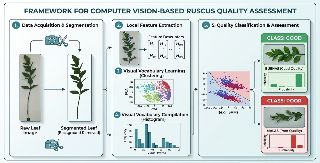
The proposed system follows a hybrid approach that combines geometric analysis and machine learning for the automated evaluation of Ruscus hypophyllum foliage. The overall pipeline consists of four main stages: (i) image acquisition under controlled conditions, (ii) image preprocessing and segmentation, (iii) stem size estimation using a geometric pixel-based method, and (iv) binary classification of foliage condition (good vs. poor) using supervised machine learning models based on Bag of Features representations [23]. Stages (i) and (ii) are shared by both downstream tasks, while stages (iii) and (iv) operate independently on the preprocessed output, allowing each attribute to be assessed using the most appropriate method for its nature. The overall architecture of the proposed system is illustrated in Figure 1.
2.1. Image Acquisition
The image dataset was obtained through a controlled acquisition process designed to ensure consistent lighting, scale, and background conditions across all samples. Images of Ruscus hypophyllum foliage were captured using a Xiaomi Redmi Note 10 Pro smartphone equipped with a Samsung ISOCELL HM2 image sensor (maximum resolution: 108 MP), operated through the Open Camera application (v1.53, Android) [25], which allows user-defined output resolutions. The camera was configured to a custom resolution of pixels, selected to cover the full length of the foliage sample and the reference marker within a single frame while maintaining adequate spatial detail for both geometric measurement and visual feature extraction.
Plant samples were placed horizontally on a flat white surface, with the camera mounted at a fixed distance ranging from 40 to 50 cm above the scene. A reference marker of known physical length was included within the field of view of each image to enable spatial calibration, compensating for any residual variation in the camera-to-sample distance across acquisitions [26]. To improve image quality and minimize shadow formation, the acquisition setup included two white LED lamps of 9 W each, providing approximately 800 lumens per lamp, arranged symmetrically on both sides of the acquisition surface to ensure uniform illumination across all captured samples. Additionally, a white background was used to facilitate the subsequent segmentation of the foliage from the background during image preprocessing.
A total of 1,500 images were initially captured. A subsequent manual quality inspection was performed to remove images exhibiting motion blur, partial occlusion of the sample, or incomplete visibility of the reference marker. Following this filtering process, 1,233 images were retained to constitute the final dataset used in all experiments.
2.2. Dataset Description
The dataset used in this study comprises 1,233 images of Ruscus hypophyllum foliage acquired during the post-harvest processing stage under the controlled conditions described in Section 2.1. Each image was annotated with respect to two independent attributes: stem size and foliage condition.
Stem size was categorized into three classes—small, medium, and large—based on the physical length of the main stem, as determined by manual measurement using a reference ruler. The length thresholds defining each category were established according to commercial post-harvest grading standards applied in the production facility [3]: stems up to 25 cm were classified as small, stems between 25 cm and 35 cm as medium, and stems between 35 cm and 45 cm as large.
Foliage condition was defined as a binary attribute—good or poor—based on visual inspection criteria. Samples were labeled as good when they exhibited uniform leaf distribution, adequate leaf density, and absence of visible damage such as yellowing, mechanical injury, or pathological symptoms. Samples were labeled as poor when one or more of these criteria were not met. Labeling was performed independently by two post-harvest workers with more than five years of experience in the classification of Ruscus hypophyllum foliage at the production facility. Both annotators applied the same visual criteria defined above to assign each sample to the good or poor condition class. Inter-annotator agreement was high, with disagreements occurring in only 5 out of 1,233 cases (0.4%). In these cases, the final label was determined by consultation with the facility’s senior agronomist, who served as the arbiter. This three-tier annotation protocol ensured consistent and traceable ground truth labels across the full dataset.
Although six combinations of size and condition can theoretically be defined, the two attributes were treated as independent tasks in the proposed framework: stem size was estimated using the geometric method described in Section 2.4, while foliage condition was classified using the machine learning models described in Section 2.6. The distribution of images across both attributes is summarized in Table 2.
The dataset presents a moderate class imbalance in the condition attribute, with 525 good samples (42.6%) and 708 poor samples (57.4%). This imbalance is representative of real post-harvest processing conditions and is addressed during model evaluation through stratified sampling, as described in Section 2.7. The dataset size is consistent with previous studies applying classical machine learning models to structured visual feature representations [19,21], where datasets of similar scale have demonstrated sufficient statistical power for reliable model comparison.
2.3. Image Preprocessing
Prior to feature extraction, all images were subjected to a four-stage preprocessing pipeline designed to improve visual quality, reduce illumination variability, and isolate the foliage region from the background. The entire preprocessing pipeline was implemented in Python using the scikit-image and OpenCV libraries [27,28]. The pipeline consists of the following stages: resizing, color space conversion, background segmentation, and image enhancement, as illustrated in Figure 2.
Stage 1—Resizing and normalization. Each image was resized so that the full length of the foliage stem was contained within the image frame, ensuring that no relevant morphological information was lost during subsequent processing. No fixed target resolution was imposed, as stem length varies across samples; instead, the resizing factor was determined individually per image to preserve the aspect ratio and guarantee complete stem coverage. Following resizing, intensity normalization was applied to reduce inter-image variability caused by minor illumination differences across acquisition sessions. Intensity normalization is a standard preprocessing step for reducing inter-image illumination variability in agricultural vision systems, where consistent feature representations are critical for reliable classifier performance [15,16].
Stage 2—Color space conversion. Each resized image was converted from the RGB color space to grayscale using a standard luminance-weighted transformation. The grayscale representation was used as the primary input for the subsequent segmentation stage. Additionally, opponent color channels—green-red and blue-yellow—were computed from the original RGB image to support visual inspection and qualitative analysis of foliage chromatic characteristics, including the detection of yellowing and color anomalies associated with poor foliage condition. Grayscale conversion reduces computational complexity while preserving the structural and textural information required for subsequent segmentation and local feature extraction [21].
Stage 3—Background segmentation. Background removal was performed on the grayscale image using Otsu’s global thresholding method [29], which automatically determines an optimal intensity threshold by minimizing the intra-class variance between foreground and background pixels. Given the controlled white background used during image acquisition, this method produced reliable binary masks across all samples. The resulting binary mask was applied to isolate the Ruscus hypophyllum foliage from the background in subsequent processing stages, using the threshold_otsu function from the scikit-image library [27]. Otsu’s thresholding has been widely validated as an effective and parameter-free background removal method in plant image analysis tasks, producing reliable binary masks under controlled white-background acquisition conditions [15,29].
Stage 4—Image enhancement and filtering. To improve the discriminability of local visual features in the segmented foliage region, contrast enhancement was applied using Contrast Limited Adaptive Histogram Equalization (CLAHE) [30], implemented via the createCLAHE function from the OpenCV library [28]. CLAHE operates on local image tiles rather than the entire image, enhancing contrast in each region independently while limiting noise amplification in homogeneous areas [30]. Following contrast enhancement, a Gaussian filter was applied using cv2.GaussianBlur to reduce high-frequency noise introduced during acquisition and contrast processing, producing a smoothed image suitable for both geometric analysis and local feature extraction. CLAHE has been shown to improve local feature discriminability in plant image classification tasks by enhancing contrast in regions with subtle visual differences [21,30], while Gaussian filtering reduces high-frequency noise that would otherwise interfere with stable keypoint detection in SIFT-based feature extraction pipelines [24]. This enhancement stage was applied uniformly to the output fed into both the geometric estimation branch and the Bag of Features classification branch of the proposed framework.
2.4. Stem Size Estimation
Stem size estimation is performed using a geometric multi-stage image processing approach implemented entirely in Python using the OpenCV library [28]. By leveraging the controlled acquisition environment, the proposed method enables the conversion of pixel-level measurements into real-world physical dimensions (mm) without relying on machine learning models, following approaches based on geometric calibration and image-based measurement reported in recent agricultural vision systems [16]. The complete pipeline for stem size estimation is illustrated in Figure 3.
2.4.1. Reference Marker Detection
A physical reference marker of known length was included within the field of view of each image during acquisition. This marker consists of a straight line segment of fixed and known physical length, positioned horizontally at with respect to the image frame. The marker was detected automatically in each image using contour detection via the cv2.findContours function, followed by blob analysis to identify the marker region based on its geometric properties, including area, aspect ratio, and compactness [28]. Once detected, the marker serves two purposes: (i) it defines the reference orientation of the coordinate system, since the marker is known to be horizontal (), and (ii) it provides the spatial calibration factor S expressed in pixels per millimeter (), computed as:
where is the detected length of the marker in pixels and is its known physical length in millimeters. This pixel-to-metric conversion approach has been widely applied in precision agriculture and plant phenotyping systems [16,17].
2.4.2. Stem Detection and Orientation Estimation
The main stem structure is identified from the segmented foliage mask by comparison with the reference marker pattern. Since the reference marker is a known horizontal line segment at , the stem region is identified as the primary elongated structure in the binary mask whose orientation deviates from the reference orientation. The inclination angle of the stem with respect to the horizontal axis is then estimated by comparing the stem’s principal axis against the reference marker direction, using contour-based bounding box analysis via cv2.minAreaRect [28]. This angular information is used to perform a deskewing operation, compensating for variations in stem inclination and ensuring a consistent geometric reference frame across all samples.
2.4.3. Trigonometric Length Correction and Size Categorization
After orientation estimation, the stem length is derived from its horizontal projection obtained from the axis-aligned bounding box. Since the stem may be inclined at angle with respect to the horizontal axis, a trigonometric correction is applied to recover the true stem length, as commonly used in vision-based measurement systems for inclined objects [31]. The corrected stem length in pixels is computed as:
where represents the horizontal projection of the stem length obtained from the bounding box, and is the inclination angle of the stem with respect to the horizontal axis. The final stem length in millimeters is obtained by applying the spatial calibration factor S derived from Equation (1):
The estimated stem length is subsequently used to assign each sample to one of three size categories according to the thresholds defined in Table 2: small ( mm), medium ( mm), and large ( mm).
2.5. Feature Extraction Using Bag of Features
Visual features were extracted using the Bag of Features (BoF) approach [23], which remains a competitive representation for image classification tasks under limited data conditions [22]. Feature extraction plays a critical role in leaf-based classification systems, where characteristics such as shape, texture, and color are commonly used to discriminate between plant samples [21]. Local feature points were detected using the Scale-Invariant Feature Transform (SIFT) detector [24], and descriptors were computed for each keypoint. SIFT was selected due to its well-established robustness to changes in scale, rotation, and illumination conditions, as well as its broad validation in plant-related image classification tasks [21,24]. The entire feature extraction pipeline was implemented in Python using the OpenCV library [28].
The extracted SIFT descriptors were clustered using the k-means algorithm [32], implemented via sklearn.cluster.KMeans from the scikit-learn library [33], to construct a visual vocabulary of words. The k-means algorithm was run with a maximum of 300 iterations and a convergence tolerance of , using ten independent random initializations to reduce sensitivity to the initial centroid placement. The selection of an appropriate vocabulary size is known to directly influence classification performance in BoF-based systems, with excessively small vocabularies producing insufficient visual discrimination and excessively large ones introducing redundancy without accuracy gains [21,23]. The optimal vocabulary size was determined through a systematic sensitivity analysis described in Section 3.2.
Each image was then represented as a histogram of visual word occurrences:
where and denotes the frequency of occurrence of the i-th visual word in the image. Prior to classification, the feature vectors were normalized using L2-normalization to ensure unit-length representations, improving numerical stability and classifier performance across models with different sensitivity to feature magnitude [19]. The overall BoF pipeline is illustrated in Figure 4.
2.6. Machine Learning Classifiers
The classification task was formulated as a binary problem, in which each foliage sample was assigned to one of two condition classes: good or poor. Several supervised machine learning algorithms were evaluated, including Decision Trees, Logistic Regression, Gaussian Naive Bayes, Support Vector Machines (SVM), k-Nearest Neighbors (KNN), and Multilayer Perceptron Neural Networks (MLP) [19,34]. For each family of classifiers, multiple configurations were evaluated by varying key hyperparameters such as kernel type for SVM, number of neighbors for KNN, distance metric, and network architecture for MLP, resulting in a total of 24 evaluated classifier configurations, as detailed in Section 3.
All classifiers were implemented in Python using the scikit-learn library (version 1.5.2) [33]. To ensure a fair and unbiased comparison between models, default hyperparameter values provided by scikit-learn were used for all configurations, with the exception of the structural parameters that define each variant (e.g., kernel type, number of neighbors, hidden layer size). This approach avoids overfitting the model selection to the specific dataset while maintaining reproducibility [19].
The selection of classical machine learning models over deep learning approaches was motivated by three main factors. First, these models are computationally efficient and interpretable, making them suitable for deployment in resource-constrained agricultural processing environments [6]. Second, deep learning approaches such as CNNs typically require substantially larger labeled datasets to achieve reliable generalization—commonly on the order of tens of thousands of samples [8,10]—whereas the present dataset comprises 1,233 images, a scale consistent with previous studies applying classical models to structured visual feature representations [19,21]. Third, classical models are particularly well-suited for handling structured feature representations such as normalized BoF histograms, where the dimensionality is moderate and the feature space is explicitly defined [19]. A direct empirical comparison between the proposed BoF-based approach and CNN-based alternatives on this dataset is acknowledged as a limitation of the present work and is identified as a priority direction for future research, as discussed in Section 4.6.
2.7. Performance Evaluation Metrics
The proposed framework is evaluated across two independent tasks, each assessed using a dedicated set of metrics: geometric stem size estimation and binary foliage condition classification.
2.7.1. Geometric Estimation Metrics
The accuracy of the stem size estimation method was evaluated by comparing the estimated stem lengths against ground truth measurements obtained manually using a physical reference ruler. Let and denote the estimated and ground truth stem lengths for the i-th sample, respectively. The following metrics were computed over all N samples:
where and is the mean absolute error. In addition to continuous measurement evaluation, a discrete size categorization accuracy is computed to assess the reliability of the three-class size assignment (small, medium, large):
where is the number of samples correctly assigned to their ground truth size class.
2.7.2. Classification Metrics
The performance of the machine learning classifiers was evaluated using four standard metrics for binary classification: Accuracy, Precision, Recall, and F1-score [35].
where , , , and denote the number of true positives, true negatives, false positives, and false negatives, respectively. Confusion matrices were additionally analyzed to provide a deeper understanding of the classification behavior of each model and to identify systematic misclassification patterns [35].
All classification results were obtained using a stratified 10-fold cross-validation scheme [19]. Stratification ensures that the proportion of good and poor samples is preserved across all folds, which is particularly important given the moderate class imbalance present in the dataset (42.6% good vs. 57.4% poor, as described in Table 2). The use of 10 folds provides a reliable estimate of generalization performance while maintaining a sufficient number of training samples per fold [19]. The reported results correspond to the mean and standard deviation of each metric computed across the 10 folds.
3. Results
This section presents the experimental results obtained for both stages of the proposed framework: geometric stem size estimation and binary foliage condition classification. Results are reported separately for each task, followed by a vocabulary size sensitivity analysis and a comparative confusion matrix analysis of representative classifiers.
3.1. Stem Size Estimation Evaluation
The performance of the proposed geometric method was evaluated by comparing the estimated stem lengths against ground truth measurements obtained manually using a physical reference ruler over all 1,233 samples in the dataset. The quantitative results are summarized in Table 3.
The proposed method achieved a MAE of 1.2 mm with a standard deviation of 0.45 mm, and an RMSE of approximately 1.3 mm, confirming the low variability and high consistency of the estimation process across all evaluated samples. The low standard deviation relative to the MAE indicates that estimation errors are uniformly distributed and do not exhibit systematic bias toward any particular stem size category.
The incorporation of trigonometric orientation correction proved essential for accurate measurement, particularly for inclined stems. Without angular compensation, the horizontal projection of the stem length systematically underestimates the true stem length due to the cosine foreshortening effect described in Equation (2). The use of the reference marker enabled a reliable and consistent conversion from pixel units to real-world dimensions via the spatial calibration factor S defined in Equation (1), ensuring measurement consistency across samples acquired at varying camera-to-sample distances.
Based on the estimated stem length , each sample was assigned to one of three size categories according to the thresholds defined in Section 2.2. Of the 1,233 evaluated samples, only 2 were incorrectly categorized, yielding a size classification accuracy of 99.84% (error rate: 0.16%). Both misclassified samples corresponded to stems with lengths near the category boundaries, where measurement uncertainty is inherently higher. These results confirm the robustness and reliability of the proposed geometric approach for accurate and interpretable stem size estimation under controlled acquisition conditions.
3.2. Vocabulary Size Sensitivity Analysis
A systematic sensitivity analysis was conducted to determine the optimal vocabulary size K for the Bag of Features representation. Classification accuracy of the Linear SVM was evaluated across under stratified 10-fold cross-validation. As illustrated in Figure 5, accuracy reaches a plateau at , 120, and 140 (92.4%) and remains stable within a narrow range (91.4%–91.8%) for larger vocabulary sizes, indicating that additional visual words beyond do not contribute meaningful discriminative information for this dataset. Values below show a consistent decrease in accuracy, confirming that a minimum vocabulary size is required to adequately capture the visual variability of the Ruscus hypophyllum foliage condition classes [21,23]. Based on these results, was selected as the vocabulary size for all subsequent classification experiments, as it achieves the peak accuracy with the smallest vocabulary size, minimizing computational cost without sacrificing performance.
3.3. Classification Performance
Table 4 summarizes the average performance metrics obtained by all evaluated classifiers using stratified 10-fold cross-validation. Classifiers are grouped by family to facilitate comparison across model types.
The results reveal a clear performance hierarchy across classifier families. SVM-based models achieved the highest overall performance, with the Linear SVM obtaining the best results across all evaluated metrics: an accuracy of % and an F1-score of %. The strong performance of linear kernel SVMs is consistent with the characteristics of the BoF feature space, where class boundaries are effectively separable using linear decision surfaces [19,36]. Furthermore, the relatively low standard deviation observed across cross-validation folds indicates stable and consistent classification behavior, reducing the risk of performance overestimation due to favorable data splits.
Within the SVM family, a clear degradation in performance is observed as the kernel complexity increases from linear to polynomial (Quadratic, Cubic) and further to Gaussian kernels. This behavior suggests that the BoF histogram feature space does not benefit from higher-order decision boundaries, and that the added flexibility of complex kernels leads to overfitting on this dataset.
MLP Neural Networks constituted the second best-performing family, with accuracies ranging from 84.8% (Three-layer) to 89.5% (Medium), slightly below the top SVM configurations. The performance gap between SVMs and MLPs may be attributed to the limited dataset size, which can restrict the generalization capability of more flexible models requiring larger amounts of training data [10].
Gaussian Naive Bayes achieved a competitive accuracy of 88.2%, outperforming several MLP configurations despite its strong independence assumption, which suggests that the BoF features exhibit a degree of statistical independence consistent with this model’s assumptions.
Logistic Regression and Decision Tree models exhibited moderate performance in the range of 82.3%–87.3% and 82.6%–85.8%, respectively, while KNN configurations consistently yielded the lowest performance across all families, with accuracies ranging from 59.9% to 70.0%. The high variability observed in KNN results (standard deviations up to %) suggests strong sensitivity to the local feature distribution generated by the BoF representation, where the assumption of proximity in feature space does not effectively capture class-discriminative patterns [19].
3.4. Confusion Matrix Analysis
To provide a deeper understanding of the classification behavior of the evaluated models, a comparative confusion matrix analysis was conducted using three representative classifiers: the best-performing model (Linear SVM), an intermediate model (Medium Neural Network), and the worst-performing model (Coarse KNN). The corresponding confusion matrices are shown in Figure 6.
The confusion matrix of the Linear SVM (Figure 6a) shows a strong concentration of samples along the main diagonal, with 480 true positives (good correctly classified) and 659 true negatives (poor correctly classified) on average across folds, yielding only 49 false positives and 45 false negatives. This reflects a well-balanced trade-off between Precision and Recall (Equations (10)–(11)), consistent with the high F1-score of % reported in Table 4.
The Medium Neural Network (Figure 6b) exhibits a moderate increase in misclassification relative to the Linear SVM, with a higher number of false positives and false negatives, indicating a less optimal decision boundary in the BoF feature space. Despite this, the model maintains an acceptable performance level with an accuracy of %, suggesting that MLP-based models can serve as a viable alternative when interpretability requirements are less strict.
In contrast, the Coarse KNN (Figure 6c) shows a substantially higher dispersion of predictions, with a large number of misclassifications in both directions. Notably, this model misclassifies a significant proportion of poor-condition samples as good, resulting in a high false positive rate that would be particularly problematic in a real post-harvest inspection scenario, where undetected poor-quality samples reaching export chains can compromise commercial reputation [3].
From a practical standpoint, the asymmetry between false positives and false negatives has different commercial implications in the post-harvest quality assessment context. A false negative (good sample classified as poor) results in unnecessary product rejection, reducing yield. A false positive (poor sample classified as good) results in defective product reaching the market, with greater commercial and reputational consequences.
4. Discussion
The experimental results obtained for both stages of the proposed framework demonstrate the effectiveness of decoupling geometric measurement from visual classification in the context of post-harvest foliage quality assessment. This section discusses the implications of the obtained results, their consistency with related work, and the limitations of the proposed approach.
4.1. Geometric Stem Size Estimation
The proposed geometric method achieved a MAE of 1.2 mm and an RMSE of approximately 1.3 mm, with a size categorization accuracy of 99.84%. These results confirm that pixel-based geometric measurement combined with spatial calibration and trigonometric orientation correction provides a highly accurate and reliable alternative to learning-based approaches for measurable physical traits under controlled acquisition conditions. This finding is consistent with previous work in plant phenotyping and precision agriculture, where geometric calibration methods have demonstrated competitive accuracy for non-destructive morphological trait estimation [14,15,16].
The orientation correction step proved particularly relevant for stems with non-negligible inclination angles. Without this correction, the cosine foreshortening effect described in Equation (2) would systematically underestimate stem length, introducing a bias that scales with the inclination angle. The use of a reference marker of known length as both an orientation anchor and a spatial calibration device addresses this challenge elegantly, without requiring additional sensors or complex camera calibration procedures [26]. This makes the proposed geometric stage particularly suitable for deployment in low-cost agricultural processing environments.
The two misclassified samples corresponded to stems with lengths near the category boundaries (i.e., close to 250 mm or 350 mm), where small measurement errors are sufficient to produce an incorrect size assignment. This behavior is inherent to any threshold-based categorization system and could be mitigated in future work by introducing a rejection region or uncertainty band around the category boundaries, allowing ambiguous samples to be flagged for manual inspection rather than assigned to a potentially incorrect category.
4.2. Foliage Condition Classification
Among the evaluated classifiers, the Linear SVM achieved the best overall performance, with an accuracy of % and an F1-score of %. This result is consistent with previous studies in agricultural image classification, where SVM-based models have demonstrated strong effectiveness in high-dimensional structured feature spaces [19,36]. The superiority of the linear kernel over polynomial and Gaussian kernels suggests that the BoF histogram representation produces a feature space where the two classes are approximately linearly separable, making the additional flexibility of non-linear kernels counterproductive due to the risk of overfitting on a dataset of moderate size.
The competitive performance of Gaussian Naive Bayes (88.2%) relative to more complex models such as MLP Neural Networks is noteworthy. This result suggests that the normalized BoF histograms exhibit a degree of feature independence that is compatible with the Naive Bayes assumption, which may be related to the relatively orthogonal nature of visual word occurrences in the vocabulary space [19]. This finding has practical implications, as Gaussian Naive Bayes is computationally inexpensive and highly interpretable, making it a viable lightweight alternative to SVM in resource-constrained deployment scenarios.
The consistently poor performance of KNN configurations (59.9%–70.0%) can be attributed to the nature of the BoF feature space. KNN relies on the assumption that samples of the same class are spatially proximate in the feature space. However, BoF histograms are high-dimensional and sparse, producing a feature space where Euclidean and cosine distances may not reliably reflect semantic similarity between samples [19]. This limitation is further evidenced by the high cross-validation variability observed for KNN models (standard deviations up to %), indicating strong sensitivity to the specific data split used in each fold.
The confusion matrix analysis revealed an important asymmetry in the classification errors of lower-performing models. In the post-harvest context, false negatives (good samples classified as poor) are commercially less consequential than false positives (poor samples classified as good), as they result in unnecessary product rejection rather than defective product reaching export markets [3]. The Linear SVM exhibited the most balanced error distribution between these two types, further supporting its selection as the recommended model for this application.
4.3. Failure Case Analysis
An examination of misclassified samples reveals two systematic error patterns in the Linear SVM output. False negatives (good samples classified as poor, Panels a–b in Figure 7) are predominantly associated with natural leaf surface blemishes and specular reflectance artifacts introduced during image acquisition. These local intensity variations generate BoF visual word distributions that partially overlap with those characteristic of damaged foliage, causing the classifier to incorrectly assign a poor condition label despite the sample meeting all quality criteria. This suggests that the current visual vocabulary may not fully disambiguate between acquisition-induced artifacts and genuine foliar damage at the local feature level.
False positives (poor samples classified as good, Panels c–d in Figure 7) are associated with subtle chlorosis and boundary geometry ambiguity, where early-stage foliar degradation produces chromatic and textural patterns insufficiently distinct from healthy foliage in the BoF representation. These cases represent inherently ambiguous samples that may also challenge human annotators, as the visual difference between early degradation and acceptable condition is minimal. From a commercial standpoint, false positives carry greater consequence than false negatives in post-harvest inspection, as they result in defective product reaching export markets [3]. Future work could address both error types through targeted data augmentation of boundary-case samples and the incorporation of color-based features explicitly designed to detect early chlorosis patterns.
4.4. Comparison with Related Work
The proposed hybrid framework achieves competitive results compared to related work in ornamental plant classification. Classification accuracies above 99% for Anthurium cultivar identification were reported in [11]; however, that study addressed a multi-class identification problem under highly controlled conditions with a single plant species, whereas the present work targets binary quality grading under the more challenging variability inherent to post-harvest foliage processing. Deep learning-based approaches for ornamental trait estimation have reported accuracies between 35% and 99% depending on the trait [13], highlighting the variability of CNN-based methods across different ornamental attributes and the difficulty of achieving consistent performance without large labeled datasets.
The present work demonstrates that classical machine learning models combined with BoF representations can achieve competitive performance (92.4%) in a practical post-harvest foliage inspection scenario, while offering significant advantages in terms of interpretability, computational efficiency, and reduced data requirements compared to deep learning approaches [8,10]. This positions the proposed framework as a practical and accessible solution for small- and medium-scale ornamental foliage producers seeking to automate quality assessment without the infrastructure requirements of deep learning pipelines.
The competitiveness of classical machine learning models under limited data conditions is supported by empirical evidence in the literature. Comparative studies have consistently shown that SVMs outperform CNNs on small-scale image datasets, while CNNs gain a decisive advantage only when training sets reach the order of tens of thousands of samples [8,10]. Specifically, experimental comparisons on image classification benchmarks have demonstrated that SVM achieves competitive or superior accuracy relative to CNN when the number of training samples is below approximately 1,000–2,000 instances, a regime in which CNN generalization is constrained by insufficient coverage of the feature space [19,20]. The present dataset of 1,233 images falls within this range, providing a principled basis for the selection of classical models. Nevertheless, the question of whether transfer learning with pre-trained CNNs—which can partially compensate for limited labeled data by leveraging features learned from large-scale datasets—would yield competitive or superior results on this specific task remains open and is identified as a priority direction for future work [10].
4.5. Practical Deployment Considerations
The proposed framework was evaluated on a standard CPU-based environment (x86_64 architecture, 2 logical cores, 12.67 GB RAM) to assess its suitability for deployment in resource-constrained agricultural processing facilities. The complete inference pipeline—encompassing image preprocessing, BoF feature extraction, and SVM classification—achieves a mean processing time of 84.2 ms per sample, corresponding to a throughput of approximately 11.9 images per second. These results confirm that the proposed system operates in near-real-time on commodity hardware without requiring dedicated GPU infrastructure, making it practically accessible for small- and medium-scale ornamental foliage producers. The use of open-source Python libraries (scikit-learn, OpenCV, scikit-image) further reduces deployment costs, as no commercial software licenses are required. The system can be deployed on a standard laptop or low-cost single-board computer connected to a consumer-grade smartphone camera, consistent with the low-cost acquisition setup described in Section 2.1.
4.6. Limitations
Despite the promising results, several limitations of the proposed framework should be acknowledged. First, all experiments were conducted under controlled acquisition conditions, including uniform white background, fixed illumination, and a dedicated reference marker. Performance may degrade under more variable real-world conditions, such as non-uniform backgrounds, varying lighting, or occlusions, which are common in field processing environments. Second, the dataset size of 1,233 images, while sufficient for the evaluated classical models, remains relatively limited for more data-intensive approaches and may restrict the generalization of the results to broader acquisition conditions. Third, the foliage condition labels were assigned through a three-tier annotation protocol; future work should compute formal inter-annotator agreement metrics (e.g., Cohen’s ) to further quantify label consistency. Fourth, the current framework does not incorporate a rejection mechanism for ambiguous samples near classification or size boundaries, which could improve the reliability of the system in practical deployment scenarios. Finally, the present work does not include a direct empirical comparison with CNN-based approaches on the same dataset. Although the dataset size of 1,233 images is consistent with the scale typically associated with classical machine learning models [10,19], the question of whether transfer learning with pre-trained CNNs—which can partially compensate for limited data—would yield competitive or superior results on this specific task remains open. This comparison is identified as a priority direction for future work.
5. Conclusions
This paper presented a two-stage hybrid computer vision framework for the automated quality assessment of Ruscus hypophyllum foliage in post-harvest processing environments. The proposed system explicitly decouples geometric stem size estimation from visual foliage condition classification, addressing a gap identified in the literature where heterogeneous quality attributes are typically treated within a single unified learning framework. This decoupling improves system interpretability, reduces model complexity, and allows each attribute to be assessed using the most appropriate method for its nature.
The geometric stem size estimation method, based on spatial calibration via a reference marker and trigonometric orientation correction, achieved a Mean Absolute Error of 1.2 mm, an RMSE of approximately 1.3 mm, and a size categorization accuracy of 99.84% over 1,233 evaluated samples. These results demonstrate that deterministic geometric methods can provide highly accurate and reproducible measurements of physical plant traits under controlled acquisition conditions, without requiring any learning-based component for this task.
For foliage condition classification, the Bag of Features representation extracted using SIFT descriptors, combined with a Linear SVM classifier, achieved an accuracy of % and an F1-score of % using stratified 10-fold cross-validation. The comparative evaluation of 24 classifier configurations across six families demonstrated that the linear separability of the BoF feature space favors SVM-based models, while KNN configurations were systematically outperformed due to their sensitivity to the high-dimensional sparse nature of histogram representations. These findings provide evidence-based guidance for model selection in structured visual feature spaces for agricultural inspection tasks.
From a practical perspective, the proposed framework offers a low-cost, interpretable, and computationally efficient solution for automated foliage quality grading, with an inference time of 84.2 ms per sample on standard CPU hardware, suitable for deployment in small- and medium-scale ornamental foliage processing facilities. The use of a consumer-grade smartphone camera and open-source Python libraries reduces the infrastructure requirements for adoption, making the system accessible to producers in export-oriented agricultural sectors such as the Ecuadorian ornamental foliage industry [2].
Future work will address the identified limitations in four directions. First, the robustness of the system will be evaluated under more challenging real-world acquisition conditions, including variable backgrounds, non-uniform illumination, and field processing environments. Second, deep learning approaches such as Convolutional Neural Networks (CNNs) will be explored as an alternative to the BoF representation, enabling a direct comparison between classical and end-to-end learning-based feature extraction strategies on the same dataset [8]. Third, data augmentation techniques will be applied to expand the training set and improve model robustness [10]. Fourth, a rejection mechanism based on classification confidence scores will be investigated to handle ambiguous samples near size category boundaries or classification decision boundaries.
Author Contributions
F.O.-L.: Conceptualization, Methodology, Software, Formal analysis, Investigation, Writing—original draft, Visualization, and overall coordination of all stages of the manuscript (lead author). F.T.-R.: Writing—review and editing, with emphasis on manuscript drafting and language refinement. D.P.: Image preparation, Data curation, Investigation, and Validation. M.H.S.: Methodological review and Writing—review and editing. D.H.P.-O.: Methodological review, Supervision, Project administration, and Writing—review and editing (style and structure). All authors have read and agreed to the published version of the manuscript.
Funding
This research received no external funding.
Institutional Review Board Statement
Not applicable.
Informed Consent Statement
Not applicable.
Data Availability Statement
The dataset used in this study is available from the corresponding author upon reasonable request.
Acknowledgments
The authors would like to thank the Laboratory of Robotics and Industrial Automation at the Universidad de las Fuerzas Armadas ESPE for the support provided during this research. As well, authors acknowledge the valuable support given by the SDAS Research Group (https://sdas-group.com/). During the preparation of this manuscript, the authors used large language model (LLM)-based writing assistance tools to support language editing, text structuring, and drafting of selected sections. The authors have reviewed, edited, and take full responsibility for all content of this publication.
Conflicts of Interest
The authors declare no conflicts of interest.
Abbreviations
The following abbreviations are used in this manuscript:
| BoF | Bag of Features |
| CLAHE | Contrast Limited Adaptive Histogram Equalization |
| CNN | Convolutional Neural Network |
| KNN | k-Nearest Neighbors |
| MAE | Mean Absolute Error |
| MLP | Multilayer Perceptron |
| RMSE | Root Mean Square Error |
| SIFT | Scale-Invariant Feature Transform |
| SVM | Support Vector Machine |
References
- Meir, S.; Philosoph-Hadas, S. Postharvest Physiology of Ornamentals: Processes and Their Regulation. Agronomy 2021, 11, 2387. [Google Scholar] [CrossRef]
- Guaita-Pradas, I.; Rodríguez-Mañay, L.O.; Marques-Perez, I. Competitiveness of Ecuador’s Flower Industry in the Global Market in the Period 2016–2020. Sustainability 2023, 15, 5821. [Google Scholar] [CrossRef]
- Franzoni, G.; Rovera, C.; Farris, S.; Ferrante, A. Packaging materials and their effect on ruscus quality changes during storage and vase life. Postharvest Biol. Technol. 2024, 210, 112789. [Google Scholar] [CrossRef]
- Ahmad, I.; Saeed, H.A.u.R.; Khan, M.A.S. Ornamental Horticulture: Economic Importance, Current Scenario and Future Prospects. In Etiology and Integrated Management of Economically Important Fungal Diseases of Ornamental Palms;Sustainability in Plant and Crop Protection; Ul Haq, I., Ijaz, S., Eds.; Springer: Cham, 2020; Volume 16, pp. 3–40. [Google Scholar] [CrossRef]
- Cubero, S.; Aleixos, N.; Moltó, E.; Gómez-Sanchis, J.; Blasco, J. Advances in machine vision applications for automatic inspection and quality evaluation of fruits and vegetables. Food Bioprocess Technol. 2011, 4, 487–504. [Google Scholar] [CrossRef]
- Liakos, K.G.; Busato, P.; Moshou, D.; Pearson, S.; Bochtis, D. Machine Learning in Agriculture: A Review. Sensors 2018, 18, 2674. [Google Scholar] [CrossRef] [PubMed]
- Blasco, J.; Munera, S.; Aleixos, N.; Cubero, S.; Moltó, E. Machine Vision-Based Measurement Systems for Fruit and Vegetable Quality Control in Postharvest. Adv. Biochem. Eng. 2017, 161, 71–91. [Google Scholar] [CrossRef]
- Kamilaris, A.; Prenafeta-Boldú, F.X. Deep learning in agriculture: A survey. Comput. Electron. Agric. 2018, 147, 70–90. [Google Scholar] [CrossRef]
- Mohanty, S.P.; Hughes, D.P.; Salathé, M. Using deep learning for image-based plant disease detection. Front. Plant Sci. 2016, 7, 1419. [Google Scholar] [CrossRef] [PubMed]
- Too, E.C.; Yujian, L.; Njuki, S.; Yingchun, L. A comparative study of fine-tuning deep learning models for plant disease identification. Comput. Electron. Agric. 2019, 161, 272–279. [Google Scholar] [CrossRef]
- Soleimanipour, A.; Chegini, G.R. A Vision-Based Hybrid Approach for Identification of Anthurium Flower Cultivars. Comput. Electron. Agric. 2020, 174, 105460. [Google Scholar] [CrossRef]
- Li, D.; et al. Four-Dimension Deep Learning Method for Flower Quality Grading with Depth Information. Electronics 2021, 10, 2353. [Google Scholar] [CrossRef]
- Afonso, M.; Paulo, M.J.; Fonteijn, H.; van den Helder, M.; Zwinkels, H.; Rijsbergen, M.; van Hameren, G.; Haegens, R.W. Automatic trait estimation in floriculture using computer vision and deep learning. Smart Agric. Technol. 2024, 7, 100383. [Google Scholar] [CrossRef]
- Minervini, M.; Scharr, H.; Tsaftaris, S.A. Image Analysis: The New Bottleneck in Plant Phenotyping. IEEE Signal Process. Mag. 2015, 32, 126–131. [Google Scholar] [CrossRef]
- Meraj, T.; et al. Computer Vision-Based Plants Phenotyping: A Comprehensive Survey. iScience 2023, 26, 108709. [Google Scholar] [CrossRef] [PubMed]
- Zhang, Y.; Wang, C.; Liu, X. A review of Vision-based crop measurement. Sensors 2021, 21, 5057. [Google Scholar] [CrossRef] [PubMed]
- Nguyen, T.T.; Vandevoorde, J.; Saeys, W. Measurement of Plant Traits Using Computer Vision: A Review of Calibration and Scaling Methods. Bot. Rev. 2024. [Google Scholar] [CrossRef]
- Franco, V.R.; Hott, M.C.; Andrade, R.G.; Goliatt, L. Hybrid machine learning methods combined with computer vision approaches to estimate biophysical parameters of pastures. Evol. Intell. 2023, 16, 1271–1284. [Google Scholar] [CrossRef]
- Kotsiantis, S.B. Supervised machine learning: A review of classification techniques. Informatica 2007, 31, 249–268. [Google Scholar]
- Hastie, T.; Tibshirani, R.; Friedman, J. The Elements of Statistical Learning: Data Mining, Inference, and Prediction, 2nd ed.; Springer: New York, 2009. [Google Scholar] [CrossRef]
- Azlah, M.A.F.; Chua, L.S.; Rahmad, F.R.; Abdullah, F.I.; Wan Alwi, S.R. Review on Techniques for Plant Leaf Classification and Recognition. Computers 2019, 8, 77. [Google Scholar] [CrossRef]
- Sultana, F.; Sufian, A.; Dutta, P. Advancements in Image Classification Using Convolutional Neural Networks: A Survey. In Intelligent Computing: Image Processing Based Applications;Advances in Intelligent Systems and Computing; Springer: Singapore, 2020; Volume 1157, pp. 1–16. [Google Scholar] [CrossRef]
- Csurka, G.; Dance, C.; Fan, L.; Willamowski, J.; Bray, C. Visual categorization with bags of keypoints. In Proceedings of the ECCV Workshop on Statistical Learning in Computer Vision, 2004; pp. 1–22. [Google Scholar]
- Lowe, D.G. Distinctive Image Features from Scale-Invariant Keypoints. Int. J. Comput. Vis. 2004, 60, 91–110. [Google Scholar] [CrossRef]
- Brewster, M. Open Camera. Android application, version 1.53. 2021. Accessed: 2024. Available online: https://opencamera.org.uk.
- Chen, H.; Zhuang, J.; Liu, B.; Wang, L.; Zhang, L. Camera calibration method based on circular array calibration board. Syst. Sci. Control Eng. 2023, 11, 2163914. [Google Scholar] [CrossRef]
- van der Walt, S.; et al. scikit-image: Image Processing in Python. PeerJ 2014, 2, e453. [Google Scholar] [CrossRef] [PubMed]
- Bradski, G.; Kaehler, A. Learning OpenCV: Computer Vision with the OpenCV Library; O’Reilly Media: Sebastopol, CA, 2008. [Google Scholar]
- Otsu, N. A Threshold Selection Method from Gray-Level Histograms. IEEE Trans. Syst. Man. Cybern. 1979, 9, 62–66. [Google Scholar] [CrossRef]
- Zuiderveld, K. Contrast Limited Adaptive Histogram Equalization. In Graphics Gems IV; Heckbert, P.S., Ed.; Academic Press: San Diego, CA, 1994; pp. 474–485. [Google Scholar] [CrossRef]
- Liu, T.; Lv, X.; Jin, M. Research on Image Measurement Method of Flat Parts Based on the Adaptive Chord Inclination Angle Algorithm. Appl. Sci. 2023, 13, 1641. [Google Scholar] [CrossRef]
- Lloyd, S.P. Least Squares Quantization in PCM. IEEE Trans. Inf. Theory 1982, 28, 129–137. [Google Scholar] [CrossRef]
- Pedregosa, F.; et al. Scikit-learn: Machine Learning in Python. J. Mach. Learn. Res. 2011, 12, 2825–2830. [Google Scholar]
- Alshammari, A.H.; Bencsik, G.; Ali, H.A. A Survey of Six Classical Classifiers. Algorithms 2026, 19, 37. [Google Scholar] [CrossRef]
- Powers, D.M.W. Evaluation: From Precision, Recall and F-Measure to ROC, Informedness, Markedness and Correlation. J. Mach. Learn. Technol. 2020, 11, 37–63. [Google Scholar] [CrossRef]
- Ahmad, I.; Alqahtani, A.; Al-Makhadmeh, Z.; Al-Amri, A. Improved Support Vector Machine Enabled Radial Basis Function and Linear Variants for Remote Sensing Image Classification. Sensors 2021, 21, 4431. [Google Scholar] [CrossRef] [PubMed]
Figure 1.
Architecture of the hybrid framework for Ruscus hypophyllum quality assessment, comprising a preprocessing stage followed by parallel geometric and BoF classification branches.
Figure 1.
Architecture of the hybrid framework for Ruscus hypophyllum quality assessment, comprising a preprocessing stage followed by parallel geometric and BoF classification branches.

Figure 2.
Image preprocessing pipeline applied to Ruscus hypophyllum foliage images. The pipeline consists of four stages: (1) resizing and normalization, (2) color space conversion to grayscale and opponent color channels, (3) background segmentation using Otsu’s thresholding, and (4) image enhancement using CLAHE and Gaussian filtering. The output is used as input to both the geometric estimation and the Bag of Features classification branches.

Figure 3.
Pipeline for stem size estimation based on geometric processing and spatial calibration. The workflow includes bounding box detection, reference marker identification, orientation correction, and pixel-to-millimeter conversion.
Figure 3.
Pipeline for stem size estimation based on geometric processing and spatial calibration. The workflow includes bounding box detection, reference marker identification, orientation correction, and pixel-to-millimeter conversion.

Figure 4.
Bag of Features extraction pipeline. Local SIFT keypoints are detected and described for each preprocessed image. Descriptors are clustered using k-means to construct a visual vocabulary of words. Each image is represented as a normalized histogram of visual word occurrences, which serves as the feature vector for the machine learning classifiers.

Figure 5.
Linear SVM classification accuracy as a function of vocabulary size K under stratified 10-fold cross-validation. Accuracy reaches a plateau at –140 (92.4%).
Figure 5.
Linear SVM classification accuracy as a function of vocabulary size K under stratified 10-fold cross-validation. Accuracy reaches a plateau at –140 (92.4%).

Figure 6.
Confusion matrices for three representative classifiers: (a) Linear SVM, (b) Medium Neural Network, and (c) Coarse KNN. Rows represent ground truth labels and columns represent predicted labels. Values correspond to aggregated counts across 10-fold cross-validation folds.
Figure 6.
Confusion matrices for three representative classifiers: (a) Linear SVM, (b) Medium Neural Network, and (c) Coarse KNN. Rows represent ground truth labels and columns represent predicted labels. Values correspond to aggregated counts across 10-fold cross-validation folds.

Figure 7.
Representative failure cases of the Linear SVM: false negatives (a–b, good misclassified as poor) caused by surface blemishes and reflectance artifacts; false positives (c–d, poor misclassified as good) caused by subtle chlorosis and boundary geometry ambiguity.
Figure 7.
Representative failure cases of the Linear SVM: false negatives (a–b, good misclassified as poor) caused by surface blemishes and reflectance artifacts; false positives (c–d, poor misclassified as good) caused by subtle chlorosis and boundary geometry ambiguity.


Table 1.
Representative studies on vision-based quality assessment of ornamental plants and related species.
Table 1.
Representative studies on vision-based quality assessment of ornamental plants and related species.
| Study | Species | Attributes | Method | Accuracy |
|---|---|---|---|---|
| Soleimanipour & Chegini [11] | Anthurium | Cultivar identification | Geometric + ML | >99% |
| Li et al. [12] | Cut flowers | Maturity/quality grading | CNN (4D deep learning) | N/R |
| Afonso et al. [13] | Ornamental floriculture | Multiple morphological traits | CNN | 35–99% |
| Franco et al. [18] | Pastures | Biophysical parameters | Hybrid ML + CV | 85–90% |
| This work | Ruscus hypophyllum | Stem size and foliar condition | Decoupled geometric + BoF/SVM | 99.84% + 92.4% |
Table 2.
Dataset distribution by stem size and foliage condition.
| Size Class | Length Range (cm) | Images | Condition | Images |
|---|---|---|---|---|
| Small | 407 | Good | 525 | |
| Medium | 413 | Poor | 708 | |
| Large | 413 | — | — | |
| Total | — | 1,233 | Total | 1,233 |
Table 3.
Quantitative evaluation metrics for the proposed geometric stem size estimation method.
| Metric | Value |
|---|---|
| Mean Absolute Error (MAE) | 1.2 mm |
| Standard Deviation () | 0.45 mm |
| Root Mean Square Error (RMSE) | 1.3 mm |
| Size Classification Accuracy | 99.84% |
| Misclassified Samples | 2/1,233 |
Table 4.
Average performance metrics of evaluated classifiers grouped by family. All results correspond to stratified 10-fold cross-validation. Accuracy and F1-score are reported as mean ± standard deviation.
Table 4.
Average performance metrics of evaluated classifiers grouped by family. All results correspond to stratified 10-fold cross-validation. Accuracy and F1-score are reported as mean ± standard deviation.
| No. | Classifier | Acc. (%) | Prec. (%) | Rec. (%) | F1 (%) |
|---|---|---|---|---|---|
| Support Vector Machines | |||||
| 1 | Linear SVM | 90.7 | 91.4 | ||
| 2 | Quadratic SVM | 89.1 | 90.1 | ||
| 3 | Cubic SVM | 86.7 | 88.0 | ||
| 4 | Fine Gaussian SVM | 77.1 | 80.0 | ||
| 5 | Mean Gaussian SVM | 69.1 | 72.4 | ||
| 6 | Coarse Gaussian SVM | 62.2 | 65.7 | ||
| Neural Networks (MLP) | |||||
| 7 | Medium Neural Network | 87.1 | 88.6 | ||
| 8 | Wide Neural Network | 86.3 | 87.2 | ||
| 9 | Two-layer Neural Network | 85.1 | 86.1 | ||
| 10 | Narrow Neural Network | 84.4 | 85.3 | ||
| 11 | Three-layer Neural Network | 81.6 | 82.9 | ||
| Naive Bayes | |||||
| 12 | Gaussian Naive Bayes | 85.7 | 86.7 | ||
| 13 | Kernel Naive Bayes | 72.7 | 76.2 | ||
| Logistic Regression | |||||
| 14 | Efficient Logistic Regression | 84.7 | 85.7 | ||
| 15 | Binary Logistic Regression | 78.6 | 80.4 | ||
| Decision Trees | |||||
| 16 | Fine Decision Tree | 82.4 | 84.8 | ||
| 17 | Medium Decision Tree | 80.6 | 82.9 | ||
| 18 | Coarse Decision Tree | 78.7 | 81.0 | ||
| k-Nearest Neighbors | |||||
| 19 | Cosine KNN | 64.5 | 65.7 | ||
| 20 | Fine KNN | 62.0 | 63.8 | ||
| 21 | Cubic KNN | 60.2 | 61.9 | ||
| 22 | Weighted KNN | 58.3 | 60.0 | ||
| 23 | Medium KNN | 56.5 | 58.1 | ||
| 24 | Coarse KNN | 52.7 | 55.2 | ||
Disclaimer/Publisher’s Note: The statements, opinions and data contained in all publications are solely those of the individual author(s) and contributor(s) and not of MDPI and/or the editor(s). MDPI and/or the editor(s) disclaim responsibility for any injury to people or property resulting from any ideas, methods, instructions or products referred to in the content. |
© 2026 by the authors. Licensee MDPI, Basel, Switzerland. This article is an open access article distributed under the terms and conditions of the Creative Commons Attribution (CC BY) license (http://creativecommons.org/licenses/by/4.0/).
Copyright: This open access article is published under a Creative Commons CC BY 4.0 license, which permit the free download, distribution, and reuse, provided that the author and preprint are cited in any reuse.


