

Submitted:
17 June 2026
Posted:
19 June 2026
You are already at the latest version
Abstract
The exact time-space correlation function of the 1D Glauber-Ising model, quenched to temperature T = 0 and on a semi-open lattice of finite size N, is obtained. This also allows to deduce the exact empty-interval probability of the dual 1D coagulation-diffusion process on a periodic finite ring and to reproduce the long-time decay of the particle concentration. These results are consistent with the generic expectations of dynamical finite-size scaling theory.
Keywords:
Glauber-Ising model
; dynamics
; ageing
; exact solution
; finite-size scaling
; reactiondiffusion process
; coagulation-annihilation process
1. Introduction
Physical ageing phenomena [5,76] may arise in a many-body system after a quench, typically from a disordered initial state, either onto a critical point where at least two physical phases become indistinguishable or else into a phase co-existence region where two macroscopic physical phases coexist. In both cases, the after-quench dynamics is a slow one, which may come from the effects of the critical-point fluctuations or else from the competition between the relaxation towards at least two distinct physical states. Microscopically, the system separates into many (correlated or ordered) clusters whose mean size is growing with time. The phenomenology of physical ageing is contained in its three defining properties, namely [70]
- 1.
- slow dynamics (relaxations are slower than might be described by simple exponentials)
- 2.
- absence of time-translation-invariance
- 3.
- dynamical scaling
and these are reflected in the properties of the (coarse-grained) order-parameter which depends on the time t and the space coordinates . For a disordered initial state, the average order-parameter vanishes, viz. . One of the most frequently studied observables is the correlation function1
whose scaling is specified here for an algebraically growing domain size and which then defines the dynamical exponentz. The exponent b is an ageing exponent, but in what follows we shall restrict to cases where . For a non-conserved order-parameter and short-ranged interactions, one has [12,13,64].2 Up to metric scale factors, the form of the scaling function is generically expected to be universal, hence independent of most of the ‘details’ of the underlying microscopic physics, see [12,20,40,63,72] for reviews. The theoretical task of finding the form of is also of practical importance since a priori knowledge of permits long-time predictions on the basis of short-time data.
The universality of functions such as permits their study via well-chosen and mathematically extremely simplified models. In this context, the celebrate Ising model continues to play an important rôle. It is defined on a chain with spin variables attached to each of its sites. At equilibrium, it is specified through the hamiltonian [46,52]
where the exchange coupling was normalised to unity. We shall be interested here in some of its non-equilibrium dynamical properties. Such a dynamics, at temperature T, may be created in a heat-bath formulation by selecting at each time step randomly a site , whose spin is updated according to the Glauber rule [33], with the rate [34]
On a discrete chain, the single-time correlator is where the average is over the thermal histories defined by Equation (3). The correlator obeys the (rescaled) equation of motion [33,34,38,54,57], with the short-hand
For an initially disordered system, one has [33,34].
Various aspects of this model have been thoroughly analysed many times [3,4,14,24,33,34,35,36,38,48,54,56,57,58,66,75], notably for where the dynamics becomes slow and obeys dynamical scaling with the exponent . In doing so, a main issue is the appropriate treatment of the constraint , which precludes the immediate application of Fourier series. A recently introduced possibility to treat this uses spatial symmetry properties [22,42], which provides a convenient way to treat the model in a finite and periodic lattice. Here we shall consider how to extend this idea to a chain which is open on one end (following an idea from [33]), find the exact correlation function in this case and shall analyse how the finite-size effects will modify the scaling (1) of the infinite-size system. This also will allow to study the influence of the boundary conditions on the form of the scaling function. One of the aims of this study is to provide an explicitly worked out case to serve as a background for more generic studies. One issue will be how to insert the results to be obtained in the context of finite-size scaling [6,25], especially for dynamics [71].
Another aspect of this problem arises from the link of the Glauber-Ising model with stochastic reaction-diffusion processes [68]. Here we shall focus on the coagulation-diffusion process, and mainly studied via the so-called empty-interval method e.g. [2,3,7,8,19,21,22,23,29,37,45,48,49,50,53,66,67,69,73,74,78]. Each site of the lattice is either empty or occupied by a single particle A. Particles can randomly hop to a nearest-neighbour site and if that site already happens to be occupied, the two particles undergo, with probability one, a coagulation reaction . In one dimension, the particle concentration decays3 for long times as [73], which makes it (i) a slow process (of which in principle the ageing can be analysed) with anomalous transport and (ii) is distinct from mean-field theories which hold for dimensions and would give [39]. It is long-established that this process is dual to the Glauber-Ising model at [65,68]. We shall be interested in extending this to finite lattices, with N sites. As we shall show, the correlation function on a semi-open lattice in the Glauber-Ising model corresponds to a the empty-interval probability on a periodic ring in the coagulation-annihilation process, from which observables such as the concentration can be found.
This paper is organised as follows. Section 2 recalls first the treatment of a finite, periodic chain in the Glauber-Ising model before the semi-open geometry is defined and then solved through an extension of the spatial-symmetry method. We also discuss if/when a natural-looking short-cut towards the scaling function is applicable. In section 3 we shall show that the correlation function of the semi-open Glauber-Ising model can be reinterpreted as the empty-interval probability on a periodic ring. Conclusions are given in section 4. Three appendices contain technical details of the calculations.
2. Correlation Functions on a Finite Chain
We now describe the calculation of the spin correlation function which will be done throughout in the continuum limit such that . We shall also restrict to since this is the only situation where dynamical scaling holds and slow dynamics occurs.
1. We begin by recalling the result in the Glauber-Ising model on a periodic ring with N sites [42]. In the continuum limit, one has from (4) for the correlation function the following equation of motion, together with the boundary conditions
and where . The first of these constraints comes from the Ising constraint in (4) and the second one comes from the periodicity. Rather than dealing with these directly, we recognise first that the physical correlation function is even in x. This means that we can restrict to positive value of x only, such that with negative spatial arguments becomes available for purely mathematical purposes. This permits to treat the two constraints in (5) by using an analytic continuation to negative values of x. From now on, will denote that analytically continued function and only at the very end, we revert to the physical correlation function by making the substitution . The analytic continuation is expressed explicitly as follows [42]
Clearly, the spatial symmetries (6) reproduce the constraints in (5). Together, these can be shown to imply that the analytically continued function is periodic in the spatial coordinate x, with period , see (6). In this way, the physically motivated constraints are embedded into spatial symmetry properties of the analytically continued function . Hence, for the analytically continued function, one has the Fourier series representation [44]
and now the equation of motion (5) can indeed be solved in Fourier space. A straightforward calculation leads for the physical correlation function to [42]
It follows that both the physical constraints as well as the required periodicity properties (6) are indeed satisfied, if they only hold for the initial correlator . If the initial correlation function decays with x, the term is irrelevant in the sense that it merely give rise to corrections to the leading finite-size scaling limit behaviour. This obtained by taking simultaneously the limits , and but such that the (finite-size) scaling variables
are kept finite. In this scaling limit, which also arises naturally for a fully disordered initial state4 where , one may re-cast the physical single-time correlator (1) as
where are distinct Jacobi theta functions [1]. This form is in generic agreement with the expectation of dynamical finite-size scaling [71]. The expressions (10) give the explicit finite-size scaling functions for the single-time correlator, in terms of the finite-size scaling variables and , for a periodic chain5 of length N.
2. Our focus shall be on the semi-open chain, see Figure 1. Herein, we already used that the correlation function , of a central spin at position and another one n sites away, is symmetric in n and we can therefore consider without restriction on the generality.6 Specifically, consider that at the leftmost edge an Ising spin is fixed and we look for the correlator with another spin at site n, to the right. The chain is open at the right end because of the requirement . In the continuum limit, we have (with )
since the leftmost spin is considered immobile. Rather than dealing with these two constraints directly, we shall implement them via spatial symmetries in an analytically continued function , in the same spirit as for the periodic case above. These conditions are chosen to be
The first of these solves the first constraint. From the definition (12) of the function , the second constraint implies
In addition, combination with the first property (12), proves that on the interval , the function B is anti-symmetric (as shown in appendix A)
Since vanishes at the extremities of the interval it can be considered to be of spatial period . Furthermore, it admits a Fourier representation ([44], Kap. 4)
which is the analogue of (7) above. Then the equation of motion (11) can be solved in Fourier space and we find (see appendix A for the details)
where finally the analytically continued function is reduced to the physical correlation function by making at the very end the substitution . This gives the exact expression for the correlation function between an Ising spin at the centre of the open segment and another spin at the position , subject to Glauber dynamics and such that the correlation function is forced to vanish at the end of the segment, see Figure 1. Up to a trivial re-scaling in time (which comes from the rescaled equations of motion) the corrections to the leading scaling forms, for both the periodic and the semi-open lattice, are the same. The leading scaling contributions can be cast into their final forms
which depend on the finite-size scaling variables and . They are both consistent with the generic expectations of dynamical finite-size scaling [71] in the sense that we can write the correlation functions (Section 2) as which generalises (1) and where the universal scaling functions are boundary-condition-dependent. The existence of a second argument is the new feature of finite geometries. In the Glauber-Ising model, spatially decaying initial correlations are always irrelevant and merely generate corrections to scaling [38,41].
Figure 2 illustrates these scaling functions: the semi-open correlator (17a) in Figure 2(a) and the periodic correlator (17b) in Figure 2(b), over against the finite-size scaling variable . This is the first time that exact results for dynamical non-equilibrium many-body system are presented for non-periodic boundary conditions. A common aspect is that the functional forms of these correlators not only depend on the second finite-size scaling variable , but on the boundary conditions as well. At first sight, their behaviour is clearly quite distinct (notice that the qualitative shape of the curves in Figure 2(b) is similar to the one found for the spherical model in dimensions, quenched a temperature [41]). Upon closer inspection, it appears that the behaviour of the semi-open correlator (17a) in the interval is quite analogous, although not identical, to the behaviour of the periodic correlator (17b) in the interval . Here the distinct boundary conditions and are of essential influence. For example, at , the semi-open correlator vanishes exactly, whereas in the periodic case, at , the correlator tends to zero exponentially fast with increasing N. On the other hand, if one considers, as in the inset of Figure 2a, the dependence of on the bulk scaling variable the scaling functions are close the one of the spatially infinite system, viz. , if is large enough.7 On the other side, if , one finds a linear decays whose slope approaches to the one of the infinite-size system, for large enough. Deviations from the infinite-size curve become first visible for large values of . That for small spatial separations, one finds a cusp at , is a consequence of the ‘hard’ Ising spins, see Figure 2 (referred to as Porod’s law [12]) – in contrast to the ‘soft’ spherical model spins, where the correlator is rounded off at ([41], Figure 1(a)).
3. Given that scaling approaches often allow for a rapid and simple derivation of (universal) scaling functions, it is tempting to try such a scaling approach for the solution of the equation of motion (11) and with its associated boundary conditions. One might try one’s hand at a simple scaling ansatz of the form
which should hold in the scaling limit where simultaneously , but is kept finite [31]. Inserting the ansatz into (11) readily gives the differential equation
and where the two constants are to be found from the boundary conditions and , implied by (11). This yields
where is the error function ([1], [(7.1.1)) and is the complementary error function. Of course, such a scaling solution will be independent of any initial correlator . Since for large arguments exponentially fast [1], the solution (20) certainly has the attractive feature that for one recovers the exactly known scaling function of the spatially infinite system [14].
Does the approach leading to (20) represent an useful short-cut in order to obtain the exact physical correlation function ? If that were so, comparison with the exact solution (17a) would imply the mathematical identity
where the last relation is a consequence of the modular transformation
which follows from Poisson’s resummation formula [47] of the Jacobi theta function ([1], (16.27.3)).
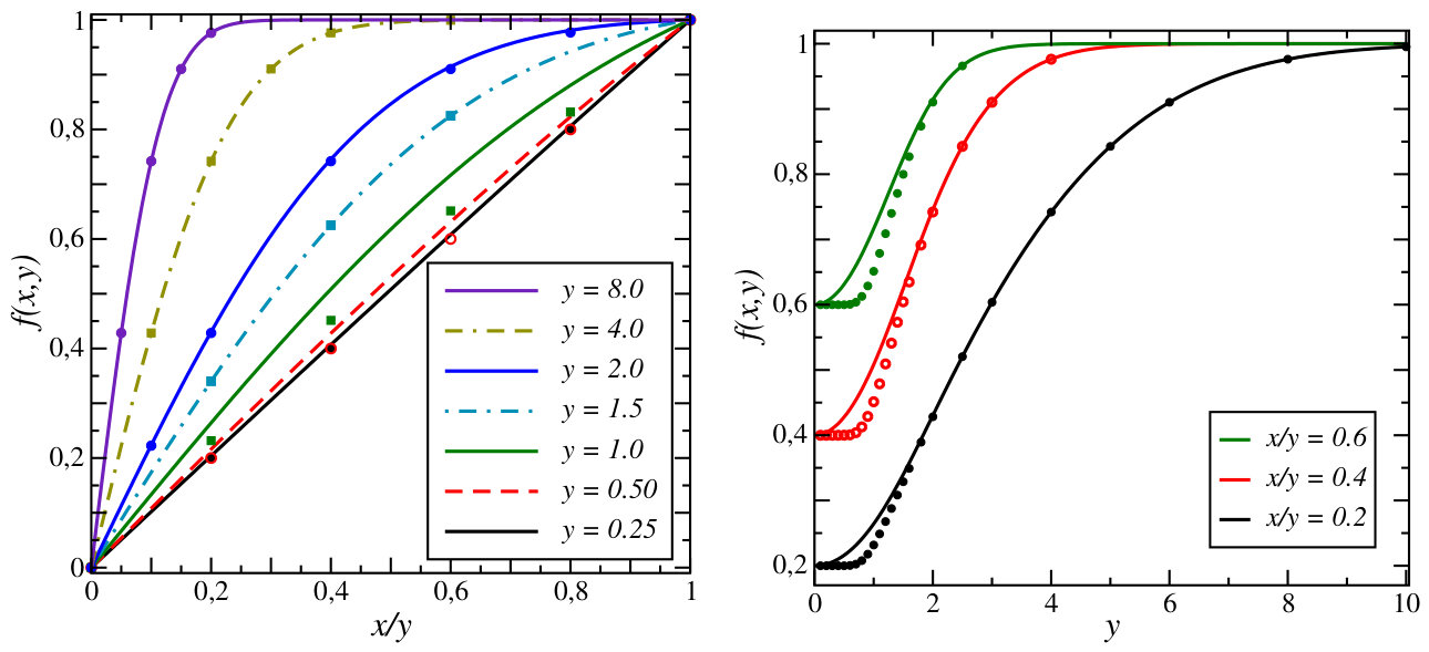
In Figure 3 numerical tests of the conjectured relation (21) are shown. In the left panel, essentially the dependence on x of the function is displayed, for several values of y. The full curves show the left-hand side of (21) as it follows from , whereas the points show the right-hand side of (21) as it follows from . Clearly, for y large enough an excellent agreement is found and the points fall very nicely onto the full lines of the same colour. However, when , notable deviations appear, which are particularly notable around . The right panel illustrates this further by showing as a function of y, for several values of . Again, for y large enough, one observes a very good agreement (the points fall clearly onto the full lines of the same colour and deviations should be exponentially small) but and lead to different results for small values of y, which appears to be most strong around . The same effect can also be seen in Figure 2(a), where the dashed gray lines give for two values of . For the more large one (blue curve), there is a very good agreement with the exact result (17a). However, for the more small one (green curve), deviations are notable, although the curves are qualitatively similar.
Hence the proposed identity (21) only holds approximately, in the region . The intriguing and simple short-cut towards a finite-size scaling function only produces an approximate result, probably since the ansatz (18) merely depends on the single scaling variable . Comparison with the exact result (17a) shows this to be an over-simplification [71]. Implicitly, in the scaling approach described here, one has admitted that but Figure 3 shows that the cross-over, when the length scale becomes comparable to N, is not well-captured.
3. Coagulation-Diffusion Process
The Glauber-Ising model at temperature is dual [65,68] to the coagulation-diffusion process, of particles of a single species A and provided diffusion and coagulation occur with the same rate.8 In the exact solution, a central quantity is the empty-interval probability [7,21,22,23,29,49], which is the probability to find an interval of n subsequent empty sites. Under the stated conditions, obeys a closed set of equations of motion. In the continuum limit, one rather deals with a function and which obeys the well-known equation of motion [8,48]
Herein, the last condition holds if the particles are moving on a ring of N sites. If initially, there is at least one particle in the system, the last particle which has survived the coagulation reactions cannot decay because of the lack of a reaction partner and on a ring of N sites, the most large empty interval can have sites. The other constraint follows since only nearest-neighbour particles can undergo a coagulation reaction. In what follows, we shall always scale to .
Clearly, the equations of motion (11) and (23), along with their constraints, are identical, up to a trivial re-scaling when going from the semi-open Glauber-Ising model to the coagulation-diffusion process. On a periodic ring of size N, the empty-interval probability can be read off from the previous discussion
This is the precise statement of the duality with Glauber-Ising chain mentioned in Section 1, for the case of finite chains with N sites. One of the quantities of interest is the time-dependent particle-concentration, which follows directly once is known [8,48] and reads
Herein, the first term does reproduce the well-known analytic result by Krebs et al. in their Equation (6.7) [49]. This already serves as an useful cross-check of our calculational technique.
The empty-interval probability can be expressed as
where is the probability to find an empty interval of size x bounded on the left by a particle. Carrying out the partial integration in (25) leads to a more compact expression for the time-dependent density (as derived in appendix B)
If initially the particles are uncorrelated and have the infinite-volume concentration , the initial probabilities on a finite ring may be chosen as
The distribution obeys the two constraints (23), as it should. On a finite lattice of size N, must be chosen such that the initial concentration takes indeed the desired value , and consistent with . Physical arguments for this form for initially uncorrelated particles of concentration are recalled in appendix C.
Alternatively, one may also start from the initial distribution [31]
which obeys the same boundary conditions as the choice (28). Then the concentration can be found via
with the theta function [1]. The scaling solution (the leading part in (25)) implicitly starts with an initial value and the modular transformation (22) does produce the expected long-time decay . If an initial concentration is chosen, the concentration will initially decay more slowly than the scaling solution and will cross over to the scaling decay once the more rapidly decaying scaling solution has become close to it.
4. Conclusions
Even a century after its introduction [46,52], and after a long history of having fruitfully stimulated many different insights into phase transitions at and far from equilibrium (for historical reviews see [9,10,27,28,32,60]), the “Ising model still thrives” [26]. We have studied here some aspects of the celebrate Glauber-Ising dynamics [33] which in turn has become quite time-honoured itself. The Glauber-Ising dynamics in is rightly famous, since it is one of the rare cases where the usually infinite hierarchy of coupled equations of motion [51,62] naturally decouples and thus becomes available to methods of analytical study. This feature has furnished explicit examples, in Ising model contexts, since a long time.
In the continuum limit, time-space-dependent correlation functions then obey simple diffusion equations but are still subject to boundary conditions which prevent a totally straightforward solution, viz. in terms of Fourier analysis. Much of the numerous work in the past decades has been on how to treat these. Our main innovation in this work has been to show how to use spatial symmetries to recast the problem into one where Fourier series methods can indeed be used and then to show how this applies in the case of non-periodic boundary conditions on finite lattices of size N. The results presented here can immediately be used as initial conditions for the calculation of two-time correlators and the exploration of novel finite-size effects therein [43,77]. We also hope that these techniques may become useful in different applications in the future, which may involve either more general interactions and/or more general boundary conditions. Similarly, in the related coagulation-diffusion process, it should be possible to consider particle currents at the boundaries [29] or to extend the techniques at hand towards the analysis of correlation functions. Again, the boundary conditions which arise in the equations of motion for the empty-interval probabilities were for a long time considered so difficult that attention was shifted to other observables which are more easy to analyse [8,48].
Explicit results were shown in Figure 2 and satisfactorily enter into the generic and expected context of dynamical finite-size scaling [71]. This also provided the opportunity to test a proposal for a short-cut towards to the dynamical finite-size scaling functions, which although not exact might become of heuristic value in more complicated systems. Numerical work will now be needed to understand further which aspects are specific to the Glauber-Ising dynamics and which ones permit further generalisation. At the very least, our result should serve as a benchmark for future numerical studies. Long-standing relations with integrable quantum chains [3,66] point towards possible extensions towards quantum dynamics [11,55,78].
Acknowledgments
It is a pleasure to thank J.-Y. Fortin for useful discussions. This work was supported by the french ANR-PRME UNIOPEN (ANR-22-CE30-0004-01).
Appendix A. Finite-Size Correlation Function
Details of the derivation of the correlation function (16) are presented.
We start from the equation of motion (11) and its two accompagning constraints for the semi-open finite chain, see Figure 1. These are parametrised using (12). Combining these leads to the condition
which upon simplification produces the anti-symmetry condition (14). Hence the unknown function is periodic on the interval and can be cast into a Fourier series (14) [44]. This implies for the Fourier coefficients
and furthermore the integral representation
Since , we find for the analytically continued correlator
Since the last factor is odd in , the constant term in the parenthesis does not contribute to the integral. We then have the decomposition
where the first continuation (12) is applied to the second line of (A5a) and ([1], (4.3.31)) was used in the second line of (A5b).
With the help of the identity
the first term in (A5c) becomes
Next, the identity
gives for the third term
such that both terms together turn into
where in the first line, the second sum is decomposed into odd and even integers and in the second line a partial cancellation arises, before the two sums can be gathered together again. With the identity , this becomes
and with the Jacobi theta function ([1], (16.27.3)). This contribution is independent of the initial correlator. Finally, the second term
can be expressed in terms of the Jacobi theta function as well. In particular, vanishes for an uncorrelated initial condition .
Appendix B. Particle-Density in the Coagulation-Diffusion Process
Equation (27) is derived. This is based on the known empty-interval probability (24) and the fact that the average time-dependent concentration can be found as the derivative [8].
We begin by considering the contribution related to the initial probability in (24). Standard trigonometric identities give
This is then inserted into the calculation of the concentration
after a partial integration. With the boundary conditions , of the empty-interval probability, the concentration becomes
To evaluate the second integral further, we recall that
hence . The usefulness of this quantity was pointed out by Durang et al. [22]. The first integral in (A13) is treated using the same boundary conditions as above. This finally implies
which is the assertion stated in the text.
Appendix C. Initial States in the Coagulation-Diffusion Process
Physical arguments to justify the use of Equation (28) are recalled.
This is done in the context of particles hopping freely on a lattice [8]. At equilibrium, one has a state of maximal entropy and particle-distribution is random (Poissonian). It may be described in terms of the so-called interparticle distribution function (ipdf) . A Poissonian distribution is exponential [8] with the particle concentration c. On the other hand, for finite times t, the ipdf is related to the empty-interval probability , namely [8,48]
where is the time-dependent concentration and the probability to find an empty interval of size x, bounded on the left by a particle. Clearly, .
If one has at equilibrium a Poissonian distribution, encoded via , it is clear that is Poissonian as well. For a spatially infinite system, which for large times relaxes towards equilibrium with , one has
reproducing the well-known form for independent particles of concentration [7,48].
On a finite chain of length L, at equilibrium the ipdf is expected to be of the form
and should be normalised according to . This fixes such that
and hence
which is (28) in the text.
One may also obtain this form via reversible coagulation-decoagulation which besides single-particle diffusion also contains the reversible reactions [21]. Therein, the empty-interval probability obeys the equation
with the decoagulation rate v. At equilibrium, one has and . With the boundary conditions and , one readily obtains [7,21]
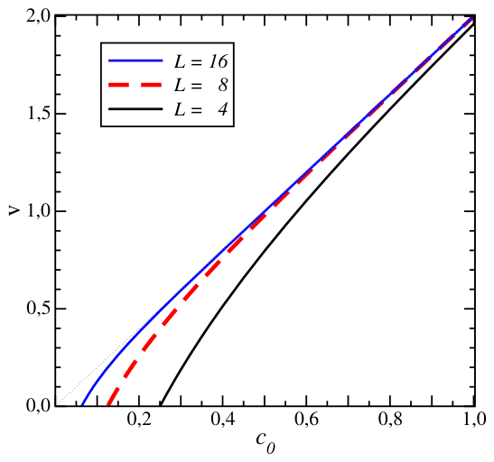
The state (28) may be achieved as follows: begin with the reversible coagulation-decoagulation process and relax it towards equilibrium, choosing by solving for v, such as to obtain the desired concentration , see Figure A1. Having fixed this configuration, the rate v for decoagulation is set to zero and the state (A22) so prepared is taken as the initial state, at time , for the subsequent irreversible coagulation-diffusion process.
Alternatively, one may also consider the statistics of a hole of n sites on a lattice of size L. This leads to the initial configuration [31]
where is the initial concentration. This satisfies the same boundary conditions as the initial configuration prepared above and is stated in (29) in the text.
Figure A1.
Choice of the parameter required for achieving the desired initial concentration , for from bottom to top.
Figure A1.
Choice of the parameter required for achieving the desired initial concentration , for from bottom to top.
References
- M. Abramowitz and I.A. Stegun, Handbook of Mathematical Functions, Dover (New York 1965).
- N. Afzal, J. Waugh, M. Pleimling, Ageing processes in reversible reaction–diffusion systems: Monte Carlo simulations, J. Stat. Mech. P06006 (2011) [arxiv:1105.3978].
- F.C. Alcaraz, M. Droz, M. Henkel, V. Rittenberg, Reaction-diffusion processes, critical dynamics and quantum chains, Ann. of Phys. 230, 250 (1994) [arxiv:hep-th/9302112]. [CrossRef]
- M.A. Aliev, Generating function of spin correlations functions for kinetic Glauber-Ising model with time-dependent transition rates, J. Math. Phys. 50, 083302 (2009).
- F. Arceri, F.P. Landes, L. Berthier, G. Biroli, A statistical mechanics perspective on glasses and ageing, in R.A. Meyers (éd.) Encyclopedia of complexity and systems science, Springer (Heidelberg 2021) [arxiv:2006.09725].
- M.N. Barber, Finite-size scaling, in C. Domb, J.L. Lebowitz (éds), Phase transitions and critical phenomena, vol. 8, Academic Press (London 1983); p. 146.
- D. ben Avraham, M. Burschka, C.R. Doering, Statics and dynamics of a diffusion-limited reaction: anomalous kinetics, noneqnilibrium self-ordering, and a dynamic transition, J. Stat. Phys. 60, 695 (1990).
- D. ben Avraham, S. Havlin, Diffusion and reactions in fractals and disordered systems, Cambridge University Press, (Cambridge 2000).
- B. Berche, M. Henkel, R. Kenna, Fenômenos críticos: 150 anos desde Cagniard de la Tour, Rev. Bras. de Ensino de Física 31, 2602 (2009). [CrossRef]
- B. Berche, M. Henkel, R. Kenna, Critical phenomena: 150 years since Cagniard de la Tour, J. Phys. Studies 13, 3201 (2009) [arXiv:0905.1886]. [CrossRef]
- I. Bouchoule, J. Dubail, Une approche hydrodynamique pour déécrire les gaz de bosons unidimensionnels, Comptes Rendus Physique 27, 253 (2026). [CrossRef]
- A.J. Bray, Theory of phase-ordering kinetics, Adv. Phys. 43, 357 (1994) [arXiv:cond-mat/9501089]. [CrossRef]
- A.J. Bray, A.D. Rutenberg, Growth laws for phase ordering, Phys. Rev. E49, R27 (1994) [arxiv:cond-mat/9303011].
- A.J. Bray, Phase-orderinmg dynamics in one dimension, in V. Privman (éd) Nonequilibrium statistical mechanics in one dimension, Cambridge Univ. Press (Cambridge 1997); pp. 143-165.
- H. Christiansen, S. Majumder, M. Henkel, W. Janke, Ageing in the long-range Ising model, Phys. Rev. Lett. 125, 180601 (2020) [arxiv:1906.11815v2]. [CrossRef]
- H. Christiansen, S. Majumder, W. Janke, Zero-temperature coarsening in the two-dimensional long-range Ising model, Phys. Rev. E103, 052122 (2021) [arXiv:2011.06098].
- F. Corberi, E. Lippiello, P. Politi, One-dimensional phase-ordering in the Ising model with space-decaying interactions, J. Stat. Phys. 176, 510 (2019) [arxiv:1902.06142]. [CrossRef]
- F. Corberi, E. Lippiello, P. Politi, Universality in the time correlations of the long-range 1D Ising model, J. Stat. Mech. 074002 (2019) [arxiv:1904.05595].
- N. Crampé, Analytical results for a coagulation/decoagulation model on an inhomogeneous lattice, Sci. Post Phys. 2, 006 (2017) [arXiv:1612.07036]. [CrossRef]
- L.F. Cugliandolo, in J.-L. Barrat, M. Feiglman, J. Kurchan, J. Dalibard (eds), Slow relaxations and non-equilibrium dynamics in condensed matter, Les Houches LXXVII, Springer (Heidelberg 2003), pp. 367-521 [arxiv:cond-mat/0210312].
- C.R. Doering, M.A. Burschka, Long crossover times in a finite system, Phys. Rev. Lett. 64, 245 (1990). [CrossRef]
- X. Durang, J.-Y. Fortin, D. del Biondo, M. Henkel and J. Richert, Exact correlations in the one-dimensional coagulation-diffusion process by the empty-interval method, J. Stat. Mech. P04002 (2010) [arxiv:1001.3526].
- X. Durang, J.-Y. Fortin, M. Henkel, Exact two-time correlation and response functions in the one-dimensional coagulation-diffusion process by the empty-interval-particle method, J. Stat. Mech. P02030 (2011) [arXiv:1012.4724].
- B.U. Felderhof, Spin relaxation in the Ising chain, Rep. Math. Phys. 1, 215 (1971); erratum 2, 151 (1971). [CrossRef]
- M.E. Fisher, The theory of critical-point singularities, in M.S. Green (ed.) Critical phenomena, Proc. 51st Int. School ‘Enrico Fermi’, Academic Press (London 1971); p. 1.
- M.E. Fisher, Simple Ising models still thrive !, Physica 106A, 28 (1981). [CrossRef]
- R. Folk, The survival of Ernst Ising and the struggle to solve his model, in Yu. Holovatch (ed.), Order, disorder and criticality, vol. 7, World Scientific (Singapour 2023); p. 1-77 [arXiv:2203.13849].
- R. Folk, B. Berche, R. Kenna, Yu. Holovatch, Ernst Ising’s doctoral thesis, World Scientific (Singapour 2026).
- J.-Y. Fortin, Crossover properties of a one-dimensional reaction-diffusion process with a transport current, J. Stat. Mech. P09033 (2014) [arXiv:1402.6901].
- J.-Y. Fortin, X. Durang, M.Y. Choi, Limited coagulation-diffusion dynamics in inflating spaces, Eur. Phys. J. B93, 175 (2020).
- J.-Y. Fortin, private communication (2026). [CrossRef]
- G.S. Girolami, A brief history of thermodynamics, as illustrated by books and people, J. Chem. Eng. Data 65, 298 (2020).
- R. Glauber, Time-dependent statistics of the Ising model, J. Math. Phys. 4, 294 (1963). [CrossRef]
- C. Godrèche, J.-M. Luck, Response of non-equilibrium systems at criticality: exact results for the Glauber-Ising chain, J. Phys. A33, 1151 (2000) [arXiv:cond-mat/9911348].
- C. Godrèche, Dynamics of the directed Ising chain, J. Stat. Mech. P04005 (2011) [arXiv:1102.0141].
- C. Godrèche, J.-M. Luck, The Glauber-Ising chain under low-temperature protocols, J. Phys. A55, 495001 (2022) [arXiv:2208.12512]. [CrossRef]
- M. Henkel, E. Orlandini, G.M. Schütz, Equivalences between stochastic systems, J. Phys. A28, 6335 (1995) [arXiv:cond-mat/9504085].
- M. Henkel, G.M. Schütz, On the universality of the fluctuation-dissipation ratio in non-equilibrium critical dynamics, J. Phys. A37, 591 (2004) [arxiv:cond-mat/0308466].
- M. Henkel, H. Hinrichsen and S. Lübeck, “Non-equilibrium phase transitions vol. 1: absorbing phase transitions”, Springer (Heidelberg 2009).
- M. Henkel and M. Pleimling, “Non-equilibrium phase transitions vol. 2: ageing and dynamical scaling far from equilibrium”, Springer (Heidelberg 2010).
- M. Henkel, Non-equilibrium relaxations: ageing and finite-size effects, Condensed Matt. Phys. 26, 13501 (2023) [arXiv:2211.03657]. [CrossRef]
- M. Henkel, Finite-size scaling in the ageing dynamics of the 1D Glauber-Ising model, Entropy 27, 139 (2025) [arxiv:2501.05912]. [CrossRef]
- M. Henkel, Physical ageing from generalised time-translation-invariance, Nucl. Phys. B1017, 116968 (2025) [arxiv:2504.16857]. [CrossRef]
- S. Hildebrand, Analysis 1, 2nd ed., Springer (Heidelberg 2006).
- H. Hinrichsen, V. Rittenberg, H. Simon, Universality properties of the stationary states in the one-dimensional coagulation-diffusion model with external particle input, J. Stat. Phys. 86, 1023 (1997) [arXiv:cond-mat/9606088]. [CrossRef]
- E. Ising, Beitrag zur Theorie des Ferromagnetismus, Z. Phys. B31, 253 (1925).
- C. Itzykson, J.-M. Drouffe, Théorie statistique des champs, vol 2, Éditions CNRS (Paris 1989);C. Itzykson, J.-M. Drouffe, Statistical field theory, vol 2., Cambridge Univ. Press (Cambridge 1989).
- P.L. Krapivsky, S. Redner, E. Ben-Naim, A kinetic view of statistical physics, Cambridge University Press (Cambridge 2010).
- K. Krebs, M.P. Pfannmüller, B. Wehefritz, H. Hinrichsen, Finite-size scaling studies of one-dimensional reaction-diffusion systems. Part I. Analytical results, J. Stat. Phys. 78, 1429 (1994) [arXiv:cond-mat/9402017], [arXiv:cond-mat/9402018].
- K. Krebs, M.P. Pfannmüller, H. Simon, B. Wehefritz, Finite-size scaling studies of one-dimensional reaction-diffusions systems. Part II. Numerical methods, J. Stat. Phys. 78, 1471 (1994) [arXiv:cond-mat/9402019].
- H.J. Kreuzer, Non-equilibrium thermodynamics and its statistical foundations, Oxford Univ. Press (Oxford 1986).
- W. Lenz, Beiträge zum Verständnis der magnetischen Eigenschaften in festen Körpern, Phys. Z. 21, 613 (1920).
- R. Li, Q. Ding, W. Cui, Scaling crossovers in non-equilibrium critical dynamics, J. Phys. A58, 385004 (2025) [arXiv:2503.05356]. [CrossRef]
- E. Lippiello, M. Zannetti, Fluctuation dissipation ratio in the one-dimensional kinetic Ising model, Phys. Rev. E61, 3369 (2000) [arXiv:cond-mat/0001103].
- N. Malvania, Y. Zhang, Y. Le, J. Dubail, M. Rigol, D.S. Weiss, Generalized hydrodynamics in strongly interacting 1D Bose gases, Science 373, 1129-1133 (2021) [arXiv:2009.06651]. [CrossRef]
- P. Mayer, L. Berthier, J.P. Garrahan, P. Sollich, Fluctuation-dissipation relations in the non-equilibrium critical dynamics of Ising models, Phys. Rev. E68, 016116 (2003) [arXiv:cond-mat/0301493].
- P. Mayer, P. Sollich, General solution for multispin two-time correlation and response functions in the Glauber-Ising chain, J. Phys. A37, 9 (2004) [arXiv:cond-mat/0307214].
- P. Mayer, P. Sollich, L. Berthier, J.P. Garrahan, Dynamic heterogeneity in the Glauber-Ising chain, J. Stat. Mech. P05002 (2005) [arXiv:cond-mat/0502271].
- F. Müller, H. Christiansen, W. Janke, Non-universality in ageing during phase-separation of the two-dimensional long-range Ising model, Phys. Rev. Lett. 133, 237102 (2024) [arxiv:2409.08050]. [CrossRef]
- M. Niss, History of the Lenz-Ising model 1920-1950: from ferromagnetic to cooperative phenomena, Arch. Hist. Exact Sci. 59, 267 (2005).
- G. Ódor, Phase transition of the one-dimensional coagulation-production process, Phys. Rev. E63, 067104 (2001) [arXiv:cond-mat/0012254].
- N. Pottier, Physique statistique hors d’équilibre, CNRS Éditions/EDP Sciences (Paris 2007).
- S. Puri, V. Wadhawan (eds), Kinetics of phase transitions, Taylor and Francis (London 2009).
- A.D. Rutenberg, A.J. Bray, Energy-scaling approach to phase-ordering growth laws E51, 5499 (1995) [arxiv:cond-mat/9409088]. [CrossRef]
- J.E. Santos, The duality relation between Glauber dynamics and the diffusion–annihilation model as a similarity transformation J. Phys. A30, 3249 (1997) [arXiv:cond-mat/9609292].
- G.M. Schütz, Exactly solvable models for many-body systems far from equilibrium, in C. Domb, J.L. Lebowitz (eds) Phase transitions and critical phenomena, vol. 19, Academic (London 2001); p. 3-251.
- D. Shapoval, M. Dudka, X. Durang, M. Henkel, Crossover between diffusion-limited and reaction-limited regimes in the coagulation–diffusion process, J. Phys. A51, 425002 (2018) [arXiv:1801.09216]. [CrossRef]
- E. Siggia, Pseudospin formulation of kinetic Ising models, Phys. Rev. B16, 2319 (1977). [CrossRef]
- H. Simon, Concentration for one and two-species one-dimensional reaction-diffusion systems, J. Phys. A28, 6585 (1995) [arXiv:cond-mat/9503128].
- L.C.E. Struik, Physical ageing in amorphous polymers and other materials, Elsevier (Amsterdam 1978).
- M. Suzuki, Static and dynamic finite-size scaling theory based on the renormalization-group approach, Prog. Theor. Phys. 58, 1142 (1977). [CrossRef]
- U.C. Täuber, Critical dynamics: a field-theory approach to equilibrium and non-equilibrium scaling behaviour, Cambridge University Press (Cambridge 2014).
- D. Toussaint, F. Wilczek, Particle-antiparticle annihilation in diffusive motion, J. Chem. Phys. 78, 2642 (1983). [CrossRef]
- L. Turban, J.-Y. Fortin, Reaction–diffusion on the fully-connected lattice: A+A→A, J. Phys. A51, 145001 (2018) [arxiv:1711.01248].
- G. Verley, R. Chétrite, D. Lacoste, Modified fluctuation-dissipation theorem near non-equilibrium states and applications to the Glauber-Ising chain, J. Stat. Mech. P10025 (2011) [arXiv:1108.1135].
- E. Vincent, Spin glass experiments, in T. Chakraborty (éd), Encyclopedia of Condensed Matter Physics, Vol. 2, pp. 371-387, Oxford University Press (Oxford 20242) [arxiv:2208.00981].
- D. Warkotsch, W. Janke, M. Henkel, Harnessing finite-size effects to gauge ageing in the 2D Ising model, submitted to J. Stat. Mech. (2026).
- A. Zahra, J. Dubail, G.M. Schütz, Emergent hydrodynamics in an exclusion-process with long-range interactions, Sci. Post Phys. 20, 141 (2026) [arXiv:2508.09879]. [CrossRef]
| 1 | It Fourier transform, the structure function, can be measured in scattering experiments. |
| 2 | |
| 3 | |
| 4 | In general, an initial correlator in (8) breaks dynamical scaling. |
| 5 | |
| 6 | The only restriction we admit is that the site is at the centre of the interval . |
| 7 | |
| 8 |
Figure 1.
Semi-open segment with N sites. At the left, an Ising spin is kept fixed and the time-dependent correlator with another spin at site is studied. The constraints and are applied.
Figure 1.
Semi-open segment with N sites. At the left, an Ising spin is kept fixed and the time-dependent correlator with another spin at site is studied. The constraints and are applied.

Figure 2.
Finite-size scaling in the Glauber-Ising model at on a finite chain for (a) semi-open and (b) periodic boundary conditions. The main plots display the dependence of the correlation function on the finite-size scaling variable , for several fixed values of . The inset in (a) shows the dependence of on the bulk scaling variable , for the same values of . The dotted line in the inset is the infinite-size correlation function . The dashed gray lines in (a) give the approximate scaling function according to (20).
Figure 2.
Finite-size scaling in the Glauber-Ising model at on a finite chain for (a) semi-open and (b) periodic boundary conditions. The main plots display the dependence of the correlation function on the finite-size scaling variable , for several fixed values of . The inset in (a) shows the dependence of on the bulk scaling variable , for the same values of . The dotted line in the inset is the infinite-size correlation function . The dashed gray lines in (a) give the approximate scaling function according to (20).
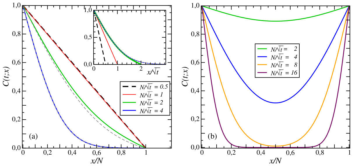
Figure 3.
Test of the identity (21), conjectured from the correlation scaling function of the finite-size semi-open Glauber-Ising model. Full curves come from the simplified scaling expression derived from . Points are derived from the exact solution . The left panel shows the dependence on for several values of y. The right panel shows the dependence on y, for several vales of .
Figure 3.
Test of the identity (21), conjectured from the correlation scaling function of the finite-size semi-open Glauber-Ising model. Full curves come from the simplified scaling expression derived from . Points are derived from the exact solution . The left panel shows the dependence on for several values of y. The right panel shows the dependence on y, for several vales of .
Disclaimer/Publisher’s Note: The statements, opinions and data contained in all publications are solely those of the individual author(s) and contributor(s) and not of MDPI and/or the editor(s). MDPI and/or the editor(s) disclaim responsibility for any injury to people or property resulting from any ideas, methods, instructions or products referred to in the content. |
© 2026 by the authors. Licensee MDPI, Basel, Switzerland. This article is an open access article distributed under the terms and conditions of the Creative Commons Attribution (CC BY) license (http://creativecommons.org/licenses/by/4.0/).
Copyright: This open access article is published under a Creative Commons CC BY 4.0 license, which permit the free download, distribution, and reuse, provided that the author and preprint are cited in any reuse.


