

Submitted:
17 June 2026
Posted:
22 June 2026
You are already at the latest version
Abstract
Cosmological tensions, most prominently the H0 and S8 discrepancies, are now understood as global consistency conditions on the underlying cosmological model rather than as isolated anomalies. We formalise this insight as a cosmological consistency triangle with three vertices that any viable cosmological model must populate simultaneously. The first two vertices, background expansion (H0) and present-day growth amplitude (S8), are universal across deviation classes. The third vertex is theory-specific: we give a formal definition that fixes it, up to reparametrisation, by the irreducible function F(z) introduced by the deviation, and demonstrate via counter-examples that the conditions have non-trivial content. We apply the framework to two contrasting deviations from ΛCDM. For f(Q) gravity, the third vertex is the growth shape, summarised by the growth index γ, against which the recent literature is surveyed. For interacting dark energy, it is the perturbation-level coupling diagnostic: we develop an original linear-perturbation analysis of the compartmentalisation model and present numerical predictions for fσ8(z) showing that the linear and non-linear coupling families are degenerate in redshift-shape at matched dimensionless coupling strength, with third-vertex discrimination acting amplitudinally in the strict quasi-static limit. From the third-vertex requirement we derive a five-point diagnostic checklist for IDE-class analyses, with brief applications to early and dynamical dark energy. The framework clarifies why background-only fits constrain at most two vertices of the triangle; DESI DR3, Euclid, the Simons Observatory, CMB-S4 and Einstein-Telescope-class sirens will decisively test whether any current proposal satisfies all three vertices simultaneously.
Keywords:
cosmological tensions
; H0 tension
; S8 tension
; f(Q) gravity
; interacting dark energy
; structure growth
1. Introduction
The standard CDM model has, for two decades, served as the working framework against which cosmological data are compared. It has accommodated successive generations of observations with no fundamental modification, from COBE through WMAP to Planck, and its parameters are now measured to sub-percent precision Planck Collaboration (2020). In the same period, however, two specific discrepancies between independent cosmological probes have grown rather than dissolved.
The Hubble-constant tension, the larger of the two, refers to a persistent disagreement between the early-universe inference from Planck CMB data Planck Collaboration (2020) and late-universe distance-ladder values clustered around . Strong-lensing time-delay measurements from the TDCOSMO collaboration TDCOSMO Collaboration et al. (2025), although somewhat broader in their statistical reach, are independently consistent with the higher value. The tension now exceeds in some dataset combinations and shows no sign of resolution by improved measurements alone.
The tension, of comparable conceptual importance though smaller in statistical magnitude, refers to the suppressed amplitude of structure growth inferred from weak-lensing surveys relative to the value extrapolated from CMB measurements under CDM. Against the Planck value Planck Collaboration (2020, ), the cosmic-shear surveys report lower amplitudes - KiDS-1000 Asgari et al. (2021, ) and DES Year 3 DES Collaboration et al. (2022, ) - a - low-side offset. Recent CMB-lensing reconstructions Qu et al. (2026) and DESI BAO measurements Abdul Karim et al. (2025) sharpen the picture without resolving it.
A community consensus, articulated most recently in the CosmoVerse White Paper CosmoVerse Collaboration et al. (2025) and the Corfu Tensions in Cosmology meeting report Di Valentino et al. (2026), is that these tensions are robust features of the data rather than artefacts of unidentified systematics. The implication is that any viable cosmological model must accommodate both, simultaneously, within current uncertainties.
This implication has, however, a structural consequence that has not been fully drawn out in the literature. Because cosmological observables are not independent - they are different functionals of the same underlying matter and metric fields - a deviation from CDM that is engineered to alleviate one tension cannot in general fail to propagate into the others. The question is not whether a candidate modification can match a preferred dataset, but whether it can simultaneously match the network of constraints set by the data as a whole. Single-tension solutions and partial-dataset analyses are therefore necessary but not sufficient elements of any genuine resolution.
We have proposed elsewhere Abebe (2026) that this requirement be formalised as a cosmological consistency triangle (CCT): three vertices that any viable cosmological model must populate simultaneously. The aim of the present paper is to give the CCT framework a fully rigorous formulation, identify its non-trivial structural content, and apply it as a model-discrimination tool to two contrasting deviations from CDM: gravity, in which the modification is gravitational, and interacting dark energy, in which the modification is non-gravitational. The two cases share the structure of the framework but differ sharply in which observable plays the role of the third vertex, and that difference is the lever through which the framework distinguishes mechanisms.
Our contribution has three components. First, we give a formal definition of the third vertex of the consistency triangle (Section 2), with three conditions that pick it out up to reparametrisation, and a counter-example demonstrating that the conditions have non-trivial content. The definition is theory-faithful: it identifies the third vertex as the observable most directly sensitive to the irreducible degree of freedom introduced by the modification, rather than to an externally specified discriminability measure. What the formal apparatus adds beyond informal “three-tension consistency” arguments is a precise sensitivity-and-orthogonality criterion that excludes plausible-looking but degenerate candidate observables (Remark 5), a unified language in which gravitational and non-gravitational deviations are compared at the level of their irreducible functions, and a diagnostic checklist that follows by direct application of the criterion rather than by stylistic preference. Second, we apply the framework to gravity (Section 3) and to interacting dark energy (Section 4), with the latter including an original linear-perturbation analysis of the compartmentalisation model of van der Westhuizen et al. van der Westhuizen et al. (2025), identifying the third vertex for non-linear dark-sector couplings. Third, we derive from the third-vertex requirement a set of necessary conditions for any IDE-class analysis to be well-posed (Section 5); these are presented neutrally as framework consequences, with citations to the literature where each condition has been satisfied or violated.
The framework is applicable beyond the two worked examples. We sketch its application to early dark energy and to dynamical dark energy (Section 6), in each case identifying the third vertex that the model’s irreducible function selects. Section 7 closes with implications for how viability claims for non-CDM models should be presented and assessed in the era of DESI DR3, Euclid, the Simons Observatory, CMB-S4, and Einstein-Telescope-class standard sirens.
2. Formalising the Consistency Triangle
Cosmological tensions, viewed individually, are points of disagreement between datasets Planck Collaboration (2020); Abdul Karim et al. (2025); TDCOSMO Collaboration et al. (2025); Qu et al. (2026). Viewed jointly, they are constraints on theory: any proposed deviation from CDM must reproduce the observed expansion history, the present-day amplitude of structure growth, and an additional quantity whose nature depends on the deviation itself CosmoVerse Collaboration et al. (2025); Di Valentino et al. (2026). The purpose of this section is to make the third requirement precise.
We proceed in five steps: identifying the irreducible function that distinguishes a deviation from CDM (Section 2.1); arguing that the first two vertices - and - are universal across deviation classes (Section 2.2); defining the third vertex (Section 2.3); reformulating the framework geometrically as a constraint surface (Section 2.4); and addressing the theory-specificity and falsifiability concerns that any such framework must answer (Section 2.5).
2.1. Setup: Irreducible Degrees of Freedom in Deviations from CDM
A deviation from CDM in the sense considered here is a one-parameter or one-functional family of cosmological models containing CDM as a particular limit. The deviation is specified by an additional dynamical object beyond what CDM contains. We call this object the irreducible function of the deviation, denoted , and we require it to be a function of cosmological redshift rather than a single number. The reason for requiring redshift-dependence is structural: any deviation specified by a single parameter is exhausted by background-level constraints alone, and the consistency-triangle question does not arise for it. The framework derives its content precisely from the fact that carries information at all redshifts.
We distinguish two broad classes of deviations by where enters the action. Gravitational deviations modify the Einstein-Hilbert action directly, replacing the curvature scalar by a function of an alternative gravitational invariant; the irreducible function is then a property of the gravitational sector itself. Examples include , , and gravity, as well as scalar-tensor theories. Non-gravitational deviations leave general relativity intact and modify the matter sector; the irreducible function is then a property of how the matter content evolves or interacts. Examples include interacting dark energy, dynamical dark energy, decaying dark matter, and early dark energy.
Three concrete examples will recur throughout this paper.
- gravity.
In the coincident gauge with the spatially flat FLRW metric, the non-metricity scalar is , and the modified Friedmann equation reads with Heisenberg (2024, ). The irreducible function is
evaluated along the cosmological history. The CDM limit corresponds to , for which .
- Interacting dark energy.
In the dark sector, energy is exchanged according to coupled continuity equations,
with the same interaction term entering with opposite signs. The irreducible function is the dimensionless coupling history
The CDM limit corresponds to . The denominator is one of several admissible choices; alternatives such as or define different parametrisations of the same family of coupling histories . The framework’s verdict on whether a model populates the consistency triangle is invariant under such parametrisation changes, even though the functional form of is not; the choice (3) is retained for definiteness and because it renders the linear-coupling case (13) the constant- case.
- Dynamical dark energy.
In the Chevallier-Polarski-Linder parametrisation, the irreducible function is
where and are the dark-energy equation-of-state parameters today and at high redshift. The CDM limit corresponds to .
In each case, is the functional handle through which the deviation acts on observables. The structure of the consistency triangle is determined by how this handle propagates into different observable quantities.
Remark 1
(Representation-awareness for higher-derivative theories). The identification of with a single function of cosmological redshift is direct for theories whose field equations are second-order in the metric. For theories with higher-derivative field equations, the dynamics requires not only the value of the modification along the cosmological trajectory but also its derivatives in the relevant scalar variable, evaluated at each redshift; the trajectory information alone is necessary but not sufficient. In such cases, is identified in a representation in which the dynamics closes on and the metric - most commonly the scalar-tensor representation, which absorbs the higher-derivative content into an additional propagating field whose cosmological history then plays the role of . The canonical example is gravity, in which the scalar-tensor representation introduces the scalaron , and the irreducible function is along the cosmological trajectory. We treat this case in Section 6, where it provides the framework’s first genuinely non-trivial stress test.
2.2. The Two Universal Vertices
Two observables are populated by every deviation, regardless of class: the background expansion rate, summarised by the Hubble constant , and the present-day amplitude of structure growth, summarised by or . The universality of these vertices is empirical: every current and anticipated cosmological dataset constrains both quantities, and any viable model must reproduce them within the data uncertainties.
Formally, the first vertex is fixed by the present-day value of the Hubble functional,
where the notation emphasises that the Hubble rate at redshift z is a functional of the entire profile for . For gravitational deviations, the dependence enters through the modified Friedmann equation; for non-gravitational deviations, through the modified energy-density evolution and the conservation equations (2).
The second vertex is fixed by the present-day amplitude of linear matter clustering,
which depends on both through the modified background - which sets the matter density evolution - and through the modified linear growth equation. In gravitational deviations, the latter modification enters via the effective gravitational coupling, e.g. in gravity Sahlu et al. (2025); Khyllep et al. (2021). In non-gravitational deviations, it enters via the coupling-induced source term in the matter conservation equation.
Remark 2.
Any viable cosmological model must satisfy both vertex 1 and vertex 2 within the current uncertainties. Failure at either vertex is sufficient for rejection. Conversely, success at both vertices is necessary but not sufficient: it leaves open the possibility that the underlying mechanism is being mimicked rather than realised. The third vertex is the apparatus by which this distinction is made.
2.3. The Third Vertex: Architectural Definition
At fixed values of vertex 1 and vertex 2, the irreducible function is not yet fully constrained: many distinct profiles produce the same and today. The third vertex is the apparatus that resolves this residual freedom by specifying an additional observable sensitive to the redshift-evolution of rather than to its integrated effect on present-day quantities.
Figure 1.
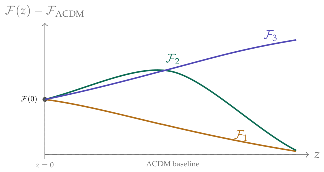
Three irreducible functions that are observationally degenerate at the first two vertices. All share the same present-day value , so they return the same , and their parameters are tuned so that the integrated effect on linear growth returns the same today; they nonetheless describe distinct cosmic histories. is a late-time monotonic deviation, is peaked at intermediate redshift, and rises to a high-redshift plateau. The first two vertices fix amplitudes, not histories; the third vertex is the observable that distinguishes the three.
Figure 1.
Three irreducible functions that are observationally degenerate at the first two vertices. All share the same present-day value , so they return the same , and their parameters are tuned so that the integrated effect on linear growth returns the same today; they nonetheless describe distinct cosmic histories. is a late-time monotonic deviation, is peaked at intermediate redshift, and rises to a high-redshift plateau. The first two vertices fix amplitudes, not histories; the third vertex is the observable that distinguishes the three.
Definition 1
(Architectural third vertex). Let a deviation from ΛCDM be specified by an irreducible function . Thearchitectural third vertexof the deviation (henceforth , or simply the third vertex) is an observable structure , which may be a single quantity or, more generally, a function indexed by additional observable parameters (such as the wavenumber k at fixed redshift, or the redshift-window at fixed scale), satisfying:
- (i)
- Sensitivity.The functional derivative is non-vanishing over a redshift range overlapping with the support of , for at least one value of μ.
- (ii)
- Quasi-orthogonality.Let denote the linear span of the functional gradients and . The component of lying in the orthogonal complement is non-vanishing, for at least one value of μ. Put simply, the third observable must carry information about that is genuinely independent of what and already constrain. Physically: there must exist at least two distinct models with identical and that nevertheless predict different values of for some μ. Any observable whose sensitivity to is fully determined by the integrated background history already captured by the first two vertices fails this condition - in particular, any smooth functional of the late-time background evaluated at alone.
- (iii)
- Operational accessibility. is measurable by current or near-future cosmological surveys with signal-to-noise sufficient to discriminate the proposed deviation from its ΛCDM limit, in at least one μ-mode when applicable.
Conditions (i) and (ii) carry the definitional content; condition (iii) carries the practical content. The two definitional conditions are logically distinct: (i) requires any non-vanishing sensitivity of to , while (ii) requires that this sensitivity not lie entirely in the directions already constrained by vertices 1 and 2. A candidate may pass (i) but fail (ii) by being functionally redundant with the present-day amplitudes, as the counter-examples below illustrate.
Remark 3
(Quasi-uniqueness, verified case by case). We do not claim a general uniqueness theorem. In each of the worked examples below (Section 3 and Section 4) and in the further applications of Section 6, conditions (i) - (iii) pick out a single observable up to obvious reparametrisations: reparametrisation of itself, smooth invertible redefinitions of (e.g. γ versus versus ), and choice of representation of the index space . The constructive identification of in each section serves as case-by-case verification rather than as appeal to a general theorem.
Remark 4
(Scale-dependence and structural enrichment of ). For deviations whose perturbation-level structure is uniform across observable scales - as in the two worked examples below ( gravity in Section 3 and interacting dark energy in Section 4) - the third vertex is a single function of redshift and the index space is trivial. For deviations whose effective gravitational coupling acquires scale-dependence, as occurs prominently in gravity through the Compton wavelength of the scalaron, the third vertex inherits this scale-dependence and becomes the wavenumber space. The framework accommodates both cases without modification of its underlying conditions; the only technical generalisation is that the conditions are required to hold for at least one μ-mode when carries μ-dependent structure. The constructive identification of in Section 3 - Section 4 and Section 6 illustrates this in three specific cases of increasing structural richness.
The argument is constructive. Given , one identifies the observable channel through which its redshift-evolution most directly enters the data. For gravity, the redshift-dependence of enters the linear growth equation through , so the third vertex is the redshift-evolution of , summarised by the growth index Mhamdi et al. (2025, ). For interacting dark energy, the redshift-dependence of enters the linear perturbation equations through coupling-dependent source terms in the continuity and Euler equations, so the third vertex is the perturbation-level coupling diagnostic, observable through the redshift-evolution of or via the integrated Sachs-Wolfe signal. Different reparametrisations of ( versus the shape of versus the time derivative of the growth rate, etc.) preserve the definitional content. We give the detailed identification of in the two worked examples in Section 3 and Section 4.
To verify that conditions (i) - (iii) are non-trivial, we exhibit a candidate “third vertex” that fails one of them.
Remark 5
(Counter-examples). For interacting dark energy, consider first the candidate , the present-day effective dark-energy equation of state. At fixed and , the late-time matter density evolution and expansion history are largely fixed, so is dominated by integrated effects already constrained by vertex 1. Two IDE models with identical background trajectories but different perturbation-level coupling histories produce indistinguishable . This is explicit: with , the present-day value depends only on the present-day value of the irreducible function, so that is supported entirely at - the region already pinned by vertex 1 - and therefore lies within , with negligible component. The candidate fails condition (ii) and does not extend the constraint surface.
A second, less trivial candidate is , the present-day deceleration parameter. This is sensitive to (condition (i)) and is measured at sub-percent level by current data (condition (iii)), yet at fixed , and it is determined by the present-day energy budget and the dark-energy equation of state at , both already in the span of vertices 1 and 2. Explicitly, for a spatially flat IDE cosmology with ,
which at fixed and is algebraically fixed. Distinct histories sharing these present-day values give indistinguishable , so the candidate again fails condition (ii). The pattern in both cases is structural: any present-day observable that is a smooth functional of the late-time background alone lies in to leading order. The third vertex must instead reach into the perturbation-level history, where the coupling diagnostic is non-degenerate.
The counter-example illustrates a more general phenomenon: the third vertex is not the “next obvious” present-day quantity, but the observable through which the redshift-evolution of most directly manifests at the level beyond the background.
2.4. The Triangle as a Constraint Surface
We can now state the central object compactly.
Definition 2
(Cosmological consistency triangle). For a deviation from ΛCDM specified by an irreducible function , thecosmological consistency triangleis the minimal three-vertex constraint system
in which and are the universal vertices fixing the present-day amplitudes, and is the theory-specific vertex fixed, up to reparametrisation, by Definition 1 from the physical channel through which departs from ΛCDM.
The geometric framing of the consistency triangle is as follows. Let denote the vector of cosmological observables, and let denote its CDM value. A deviation specified by traces a curve through observable space, parametrised by the strength of the deviation. The first two vertices select two coordinates of this curve - and - and require them to coincide with the data-preferred values within uncertainties. This defines a constraint surface of codimension two in the finite-dimensional parametrisation appropriate to the worked examples below, where is determined by between one and three free parameters; strictly, the space of admissible profiles is infinite-dimensional and the codimension language refers to constraints on any chosen finite-dimensional parametrisation thereof, extending to non-parametric by reading “codimension n” as “n independent functional constraints”.
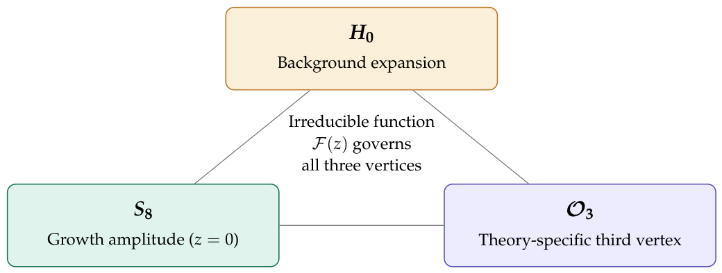
As shown in Figure 2, the third vertex selects one additional coordinate of the curve, chosen to be orthogonal in the sense of Section 2.3 to the first two. The constraint surface defined by all three vertices has codimension three, leaving in the typical case a one-dimensional locus of viable parameters within the deviation’s parameter space, or possibly an empty locus if the three vertices cannot be simultaneously satisfied.
A model is on-triangle if its irreducible function lies on this codimension-three surface within current uncertainties; off-triangle otherwise. Off-triangle models are not necessarily falsified, since uncertainties are finite, but they are disfavoured.
The codimension structure clarifies why the consistency triangle has discriminating power that single-vertex or two-vertex analyses lack. A model fitting alone is constrained at codimension one; one fitting and together is constrained at codimension two; one fitting all three vertices is constrained at codimension three. The third vertex provides one extra unit of empirical traction, and that unit is precisely what is needed to discriminate among models that pass the first two vertices through the same numerical values of and today. Two models with identical first-two-vertex projections but different irreducible functions generically separate at the third vertex.
The codimension structure just described corresponds to the simplest case, in which the third vertex is a single observable quantity. When carries additional observable structure - for example, scale-dependence inherited from a scalaron-mass transition in scalar-tensor representations of higher-derivative theories - each independent observable mode contributes its own constraint, and the codimension of the constraint surface is correspondingly higher. This is a strengthening of the framework’s discriminating power, not a weakening: a theory whose third vertex is scale-dependent must satisfy the third-vertex constraint at every observable scale, a strictly stronger requirement than satisfying it at a single scale. The two worked examples in Section 3 - Section 4 occupy the simplest corner of this structure, with trivial and codimension three; the application sketched in Section 6 occupies the first non-trivial extension, with the wavenumber space and codimension correspondingly enhanced.
Figure 2.
The generalised cosmological consistency triangle. The first two vertices, and , are universal across deviations from CDM. The third vertex is theory-specific, determined up to reparametrisation by Definition 1 from the irreducible function of the deviation. Worked examples in Section 3 and Section 4 fix and respectively, with the growth-shape diagnostic in both.
Figure 2.
The generalised cosmological consistency triangle. The first two vertices, and , are universal across deviations from CDM. The third vertex is theory-specific, determined up to reparametrisation by Definition 1 from the irreducible function of the deviation. Worked examples in Section 3 and Section 4 fix and respectively, with the growth-shape diagnostic in both.
2.5. Theory-Specificity of the Third Vertex
We now address two related concerns: that the third vertex’s theory-specificity makes the framework circular or unfalsifiable, and that an alternative, data-driven definition might be preferable.
The data-driven alternative - which we call the operational definition - would specify the third vertex as the observable that, for a given deviation, maximises some pre-specified discriminability measure between the deviation and CDM. This is intuitive but introduces ambiguities. The choice of discriminability measure (likelihood ratio, Fisher information, Kullback-Leibler divergence, posterior odds) is not unique, and different choices yield different “third vertices” for the same theory. The operational definition also averages over theories: two theories with similar background-plus-amplitude signatures but different perturbation-level mechanisms could be assigned the same operational third vertex, obscuring rather than revealing their physical distinction. The framework loses discriminating power precisely where it is most needed.
The definition (Section 2.3) avoids both problems by being theory-faithful: is determined by the irreducible function of the theory, not by an external discriminability criterion. Different theories may pick different third vertices because they introduce different mechanisms; the framework reflects the underlying physics rather than abstracting it away. The framework does not, however, require that distinct mechanisms select distinct observables: as the worked examples in Section 3 and Section 4 show, gravity and IDE both activate the redshift-evolution of , but through structurally different physical channels (a redshift-dependent effective gravitational coupling in , coupling-induced source terms in the dark-sector continuity equations in IDE). The specificity therefore lies at the level of mechanism rather than of observable in these two cases. A successful third-vertex test for a given deviation must accordingly identify not only the observable but the physical channel through which the deviation acts, since two theories that share a third-vertex observable can be discriminated only by the shape of its response. The application in Section 6, where the third vertex carries scale-dependence absent in and IDE, illustrates that distinct mechanisms can also separate at the level of observable structure.
This raises the falsifiability concern. If the third vertex is theory-specific, what prevents a theorist from choosing it so as to make the theory pass the test? The answer is that the definition is not a free choice: Conditions (i) - (iii) of Definition 1 constrain tightly enough that, in each of the worked examples below, the eligible observable is determined up to reparametrisation (Remark 3). A theorist who picks an observable that fails any of the three conditions is not specifying a valid third vertex but an arbitrary one; the consistency-triangle test is then not satisfied. The counter-example in Remark 5 illustrates how a plausible-looking choice can fail condition (ii); analogous failures of conditions (i) and (iii) are easily constructed. The framework therefore imposes a non-trivial constraint on what counts as a viable test of a deviation, and theories can fail this constraint.
In summary, the definition is preferred because it is theory-faithful, reflecting the physics of the deviation rather than abstracting it away; because it is determined up to reparametrisation by Definition 1 and its three conditions, leaving no freedom for the theorist to evade the test; and because it generalises naturally to any deviation specified by an irreducible function , without prior commitment to a particular discriminability measure. The remainder of this paper applies the framework to gravity (Section 3) and to interacting dark energy (Section 4), demonstrating in each case how the third vertex is identified and how the resulting consistency-triangle test bites.
3. Worked Example I: Gravity
We apply the framework to gravity, identifying its irreducible function and third vertex, and surveying the recent literature against the resulting constraints. The treatment here is more compact than in the proceedings version Abebe (2026) because the formal apparatus is now in place; we focus on those features specific to the realisation of the consistency triangle.
3.1. The Irreducible Function
The action of gravity in the symmetric teleparallel formulation is Heisenberg (2024)
where Q is the non-metricity scalar. In the spatially flat FLRW geometry with the coincident gauge - “Connection I” in the recent classification of admissible homogeneous and isotropic connections Ayuso et al. (2025) - the non-metricity scalar reduces to , and the modified Friedmann equation reads
At the linearly perturbed level, in the quasi-static, sub-horizon limit relevant for and weak-lensing data, the matter density contrast obeys
Equations (10) - (11) make explicit that a single function - namely evaluated along the cosmological history - governs both the background evolution and the linear growth of perturbations. This identification is precisely the irreducible function defined in equation (1). The CDM limit corresponds to .
3.2. Derivation of the Growth-Shape Vertex
We now apply Definition 1 to identify the third vertex.
The first two vertices populate as follows. The Hubble constant depends on through the integrated effect of equation (10); the present-day amplitude depends on both through the modified background and through the present-day value of , which equals .
The third vertex must (Definition 1) be sensitive to the redshift-evolution of rather than to its integrated effect or its present-day value alone. The natural candidate is the redshift-evolution of the linear growth rate, summarised by the growth index defined through , or equivalently by the shape of . This satisfies:
- (i)
- Sensitivity: is non-vanishing throughout the redshift range where is measured.
- (ii)
- Quasi-orthogonality: at fixed and , distinct profiles produce distinct values of , because is set by the time-derivative of rather than by its present-day value.
- (iii)
- Operational accessibility: is constrained by RSD and weak-lensing data with current precision , sufficient to discriminate predictions from the CDM value .
By Remark 3, the third vertex of gravity is therefore the growth shape, indexed equivalently by or by .
3.3. Confrontation with Current Data
Recent analyses of the three best-studied functional families - power-law, exponential, and logarithmic - can be read against the consistency triangle as follows.
The Bayesian study of three representative models by Boiza et al. Boiza et al. (2025), using cosmic chronometers, Type-Ia supernovae, gamma-ray bursts, BAO and CMB distance priors, finds that most analysed models yield values higher than the PlanckCDM baseline, achieving a partial alleviation of the first-vertex tension. The same paper identifies one branch satisfying that simultaneously predicts values compatible with weak-lensing measurements, but at the price of mild internal inconsistencies between subsets of data which limit the overall preference relative to CDM. The Mhamdi et al. analyses Mhamdi et al. (2024) report the exponential branch favoured over both the power-law case and CDM on a Pantheon++RSD subset, but this preference is reversed when CMB and GRB data are added - a textbook illustration of why partial-dataset verdicts do not survive the full first-two-vertex constraint.
For the third vertex, the dedicated growth-index analysis of Mhamdi et al. Mhamdi et al. (2025) reports for gravity. This is slightly above the CDM value , with the suppressed-growth values - at which late-time growth-suppression analyses claim to alleviate the tension lying within roughly of the central value but outside the preferred region. gravity therefore occupies an awkward intermediate position along the growth-shape vertex: its preferred is consistent with CDM and with a partial alleviation, while the suppressed values needed to fully resolve the growth tension are not preferred by current data and would require either a sharper measurement of or a model variant that pushes the posterior in that direction. The growth-of-structure analysis of Sahlu, de la Cruz-Dombriz and Abebe Sahlu et al. (2025) confirms that the power-law family remains observationally viable once expansion and growth data are jointly imposed, but with the exponent n forced very close to the STEGR limit .
The non-coincident sector adds further constraints. The recent DESI DR2 analysis of Paliathanasis Paliathanasis (2025), employing a non-coincident formulation in which the power-law model is recast as an effective two-scalar quintom, finds a best-fit and a smaller than CDM, with weak Bayesian evidence in favour of when GRB data are included. The De-Paliathanasis paper De and Paliathanasis (2026) provides exact non-coincident solutions including CDM-mimicking, Chaplygin-gas and CPL branches, demonstrating that the non-coincident sector admits a richer solution space than the coincident gauge.
For the gravitational-wave sector, Nájera et al. ájera et al. (2023) forecast that mock Einstein-Telescope and LISA standard sirens combined with current SNIa and BAO data could pin to better than and predict deviations exceeding at for the logarithmic class. Su et al. Su et al. (2025) reach a complementary verdict across power-law, exponential, and hyperbolic-tangent variants: their mixed model is already disfavoured by current electromagnetic data, while two hyperbolic-tangent constructions will be excluded outright by Einstein-Telescope-class siren samples. Cross-cutting probes such as standard sirens and time-delay strong lensing do not constitute an independent vertex of the consistency triangle, but rather provide simultaneous tests of multiple vertices: time-delay lensing measures directly via TDCOSMO Collaboration et al. (2025, ) while the gravitational-wave luminosity-distance ratio tracks the redshift evolution of the modified gravitational coupling.
The synthesis is straightforward. models can alleviate the tension partially, and a narrow branch can simultaneously raise and reduce towards weak-lensing-preferred values. But no single model in the literature provides a fully simultaneous, statistically preferred resolution along all three vertices (, , ) of the consistency triangle. The framework here clarifies why this should be expected: a single function controls all three vertices, and matching all three simultaneously is a strictly stronger constraint than matching any pair.
4. Worked Example II: Interacting Dark Energy
We now apply the framework to interacting dark energy (IDE). The case is structurally distinct from gravity: the modification leaves general relativity intact and acts instead through an energy-transfer term in the dark-sector continuity equations. The third vertex therefore lies in a different observable channel - the perturbation-level coupling diagnostic - rather than in the redshift-evolution of an effective gravitational coupling. We give the field-equation setup (Section 4.1), introduce two representative model families (Section 4.2), identify the irreducible function (Section 4.3) and the first two vertices (Section 4.4), and derive the third vertex (Section 4.5). The final two subsections apply the framework to the two model families: a literature-anchored treatment of the linear coupling (Section 4.6) and an original linear-perturbation analysis of the compartmentalisation model (Section 4.7).
4.1. Coupled Background Equations and Sign Conventions
Following the standard formulation Wetterich (1995); Amendola (2000); Gavela et al. (2009); Di Valentino et al. (2020), we consider a dark sector composed of cold dark matter (DM) and a dark-energy fluid (DE), coupled through a four-momentum exchange that satisfies . Restricting to scalar exchange aligned with the cosmological four-velocity, , the background continuity equations in cosmic time read
with the convention that corresponds to energy flowing from the dark-energy sector to the dark-matter sector, and conversely. The Friedmann equation is unchanged from its CDM form: , where and denote baryonic and radiation contributions. We assume the coupling is restricted to the dark sector throughout, since couplings involving baryons face stringent fifth-force constraints and require independent justification.
The sign convention in equation (12) is consequential and is one of the items we will return to in the diagnostic checklist of Section 5. With , the dark-matter density evolves more slowly than (energy is replenished from the DE sector), and the dark-energy density evolves with an effective equation of state that is less negative than the bare w.
4.2. Two Representative Model Families
- Linear coupling.
The canonical and most-studied form of the coupling is Amendola (2000); Di Valentino et al. (2020)
with a dimensionless coupling constant. For w approximately constant near , equation (13) produces an analytically tractable background and has been the workhorse of IDE phenomenology. The CDM limit corresponds to , .
- Non-linear coupling and compartmentalisation.
A broader class of couplings, in which the dark-sector exchange depends non-linearly on the dark-fluid densities, has been studied since Caldera-Cabral et al. (2009) and forms the structural basis of the recent compartmentalisation framework van der Westhuizen et al. (2025). We adopt as a representative form
which is homogeneous of degree one in the combined dark-sector density and reduces, in the limits and , to the linear forms and respectively. The functional form (14) is broad enough to capture the qualitative features of compartmentalised dark-sector models van der Westhuizen et al. (2025) while remaining analytically tractable at the perturbed level. We treat it here as one representative of the broader compartmentalisation class rather than as the unique realisation of van der Westhuizen et al. (2025); the third-vertex argument below depends on the structural property that carries an explicit contribution, which is shared by any non-linear coupling that is non-degenerate in , and is therefore robust within the class. The CDM limit corresponds to .
The two families differ in a structural respect that will be central to the perturbation analysis below: the linear coupling depends on alone, so its perturbation involves only , while the non-linear coupling depends on both densities, so its perturbation involves both and with non-trivial coefficients. The third vertex turns out to be sensitive precisely to this distinction.
4.3. The Irreducible Function for IDE
The irreducible function specified in equation (3),
takes the values (constant) and (redshift-dependent through the matter density evolution) for the two model families. Note that is a non-trivial function of redshift even when is a constant: the redshift-dependence is induced by the non-linearity of the coupling and is precisely what activates the third vertex in the non-linear case.
4.4. The First Two Vertices for IDE
The first vertex populates through the modified background. Solving equation (12) with the linear coupling (13) gives, for constant and w,
which deviates from the CDM behaviour at late times. The Hubble rate inherits this deviation through the Friedmann equation, and the inferred value can be shifted by several percent for Di Valentino et al. (2020, ).
The second vertex populates through the modified linear growth. Although the gravitational coupling is unmodified ( in IDE), the matter-conservation equation acquires a coupling-induced source term, which propagates into the perturbation equations. We treat the perturbation-level structure carefully in the next subsection, since it is the apparatus through which the third vertex is identified, but we note here that the present-day growth amplitude is in general shifted by the coupling and admits both upward and downward shifts depending on the sign of .
4.5. The Third Vertex: Perturbation-Level Coupling Diagnostic
We now derive the third vertex for IDE by linear perturbation theory. We work in the conformal Newtonian gauge with metric perturbations and and assume, for simplicity and consistency with most of the IDE literature, the absence of anisotropic stress so that . Density and velocity perturbations of species i are denoted and respectively, the latter being the divergence of the fluid three-velocity.
We adopt the dark-matter rest frame, , which is the conventional choice in IDE analyses Gavela et al. (2009) and ensures that the coupling-induced source vanishes from the dark-matter Euler equation, leaving a single coupling source in the dark-energy Euler equation. This choice fixes below as a velocity-difference term , which is subdominant in the regime retained throughout.
The perturbed continuity equations following from (12) are Gavela et al. (2009)
where is the dark-energy effective sound speed. The accompanying Euler equations, in the dark-matter rest frame, read
so that the coupling source appears only in the dark-energy Euler equation and is proportional to the velocity difference.
The third vertex is identified by examining the action of on the perturbation equations. The coupling enters equations (17) - () both through its background value (which renormalises the friction term in the continuity equation) and through its perturbation (which appears as a source), so that the redshift-evolution of modifies both the amplitude and the shape of the matter growth function. We work throughout in the quasi-static, sub-horizon limit, which we now state explicitly. The sub-horizon assumption lets spatial gradients dominate Hubble friction, ; the quasi-static assumption renders time derivatives of the metric potentials subdominant to their gradients, , so that terms of order are retained relative to time derivatives of and . Three consequences follow: there is no anisotropic stress in IDE, so ; the Poisson equation closes the metric; and for a dark-energy effective sound speed the dark energy does not cluster on sub-horizon scales, so and follows adiabatically, whereas for the dark-energy perturbations cluster and the analysis must be extended. Within this approximation, equation (17) reduces, after using this Poisson constraint and the dark-matter Euler equation (19) in the same limit, to a modified growth equation of the schematic form
where are coupling-induced terms that depend on and its derivatives. The detailed forms of depend on the model and are derived for the two specific families in the next two subsections.
The third vertex is then identified, by direct application of Definition 1, as the redshift-evolution of , summarised by the growth index or by the redshift-derivative . Specifically:
- (i)
- Sensitivity: is non-vanishing throughout the redshift range where deviates from zero, owing to the terms in equation (21).
- (ii)
- Quasi-orthogonality: at fixed and , distinct profiles produce distinct shapes. This is because the present-day amplitude is set by the integrated effect of for , while the shape is set by the redshift-derivative of , which is not fixed by the integrated value.
- (iii)
- Operational accessibility: is measured by RSD in galaxy redshift surveys with current precision at , and by ISW-galaxy cross-correlations and CMB-lensing reconstructions at intermediate redshifts.
The third vertex of IDE is therefore the same observable channel as in gravity - the redshift-evolution of - but the underlying physics is different. In gravity, the channel is activated through the redshift-evolution of . In IDE, it is activated through the coupling source terms in the dark-sector continuity equations. The sameness of the channel is a coincidence arising from the dominance of in current growth-data constraints; the underlying mechanisms are distinct.
We now apply this identification to the two model families.
4.6. Application to the Linear Coupling
For the linear coupling (13), is constant, and the perturbation in the quasi-static limit. The coupling-induced terms in equation (21) take the explicit forms
The friction term slows or accelerates the growth of depending on the sign of , while couples the matter growth to the dark-energy perturbation. Both terms are proportional to , which grows monotonically from negligible values at high redshift to order unity at the present epoch. The coupling effect on therefore turns on at low redshift, generating a redshift-shape signature in addition to a present-day amplitude shift. This is consistent with the well-established literature on IDE perturbation theory Gavela et al. (2009); Di Valentino et al. (2020): the linear coupling activates the third vertex through both amplitude and shape, and IDE analyses that retain only the background-level effect of have not constrained the third vertex.
4.7. Application to Compartmentalisation
The non-linear coupling (14) demands a more involved perturbation analysis. We carry it through here, in the form needed for the CCT analysis, and identify the resulting third-vertex signature.
- Background.
The function is non-trivially redshift-dependent, interpolating between at high redshift (where dominates) and at present. The redshift-derivative of is therefore non-vanishing throughout the matter-dark-energy transition era and is positive (i.e., the coupling weakens at late times) for the natural sign .
- Linearisation of the coupling.
Writing and expanding equation (14) to linear order in the perturbations,
where is the background coupling, and the dimensionless dark-sector fractions are
Note that at all redshifts. The notational convention adopted here is that is the fraction of species X in the dark sector, so at high redshift (deep matter era) and today. The coefficient of in equation (23) is (the other species’ fraction); this is a structural consequence of the homogeneity of degree one of in the dark-sector densities, since .
The crucial structural feature is that contains an explicit dependence on , with coefficient , that is absent from the linear coupling. This term enters the right-hand side of equation (17) and produces an additional friction term, beyond , in the growth equation for .
- Modified growth equation.
Substituting equation (23) into the perturbation equation (17) and proceeding to the quasi-static, sub-horizon limit (so that and metric-time derivatives are subdominant), we obtain
where in the second equality we have used the constraint . Combining with the Euler equation in the same limit and the Poisson equation, the resulting growth equation for takes the form of equation (21) with the explicit coefficients
The compact form exhibits the structural feature directly: the friction is the product of the two dark-sector fractions, peaked at (matter-dark-energy equality, in the fiducial model), vanishing both at high redshift () and in the limit of complete dark-energy domination ().
The subleading correction in equation () arises from second-order terms in propagated through the perturbed Friedmann constraint; it carries the same sign as the leading term and is suppressed relative to it by a further factor , which is small for over the redshift range of interest. We retain only the leading term throughout, and in the numerical implementation below we set .
- Comparison with the linear case.
The non-linear coupling produces three distinct features absent in the linear case (22):
- 1.
- The friction term has a non-monotonic redshift profile, peaked at matter-dark-energy equality, in contrast to the linear coupling’s which is monotonically increasing in magnitude towards low redshift.
- 2.
- A non-vanishing renormalisation of the gravitational source term appears in principle, representing an effective modification of the gravitational coupling induced by the coupling rather than by gravity itself. This effect mimics (but is not identical to) a modified-gravity signature. Within the small- regime relevant for current data, is subleading and is set to zero in the numerical figure below.
- 3.
- The cross-coupling to inherits the factor and vanishes in the strict QS limit with (); for this term reactivates and offers an additional discrimination channel.
The combined effect on admits two natural comparisons with the linear case, illustrated in Figure 3. At matched dimensionless coupling strength (), the linear and non-linear couplings produce predictions whose present-day deviations from CDM are of comparable magnitude (in the worked example, for the linear case versus for the non-linear case at ), with redshift-shapes that are similar in the strict quasi-static, no-DE-clustering approximation: the redshift-derivative of the deviation at matches to within between the two cases. At matched present-day irreducible function (, which requires ), the non-linear coupling activates more strongly at all redshifts and produces a that is approximately three times larger than the linear case, with at also enhanced by a factor of order . The honest finding within this approximation is that the third-vertex discrimination is amplitudinal rather than primarily shape-based: the two coupling families track each other in redshift-shape, but yield different overall deviation amplitudes depending on the normalisation chosen for comparison.
- Third-vertex signature.
The redshift evolution of in the compartmentalisation model is, by Definition 1, the third vertex. It satisfies sensitivity ( is non-vanishing throughout the matter-dark-energy transition era), quasi-orthogonality (two compartmentalisation models with the same and today but different produce curves that differ at higher redshifts, since the coupling acts through the integrated history of and not only its present-day value), and operational accessibility (RSD at is precisely the relevant redshift window). The two coupling families separate at the third vertex primarily through the amplitude of relative to a chosen normalisation, with the redshift-shape difference being a subdominant signature in the strict QS limit. Distinguishing them sharply requires either dedicated precision in the joint posterior, or extensions of the analysis beyond the strict QS limit - for example, finite dark-energy effective sound speed allowing to cluster, in which case the cross-coupling ceases to vanish and the two cases acquire additional shape distinction through equation (21).
A falsifiable consequence remains. For any given fit to background-plus- data, the linear and non-linear couplings predict different posterior values of and corresponding to the same shape; the choice between them is then made by independent measurements at the perturbation-level coupling diagnostic (e.g. via the scale-dependence introduced by , by ISW-galaxy cross-correlations, or by joint CMB-lensing reconstructions) which are sensitive to the dark-energy clustering channel beyond what the strict QS limit captures.
The analysis here makes evident that any background-only confrontation of the compartmentalisation model with data - including the recent DESI DR2 analysis of van der Westhuizen et al. (2025) - constrains only the first two vertices. The third vertex remains to be tested in dedicated analyses or in joint background-plus-perturbation Bayesian fits. Such analyses, when performed, should report posteriors not only on but also on the redshift-shape of as predicted by the perturbation analysis above.
5. A Diagnostic Checklist for IDE-Class Analyses
The framework developed in Section 2 and applied to interacting dark energy in Section 4 implies a set of necessary conditions that any IDE-class analysis must satisfy in order to constrain the consistency triangle. We collect these here as a diagnostic checklist. The conditions are framework consequences, not stylistic preferences; failure to meet any one of them implies that the analysis has not constrained at least one vertex, and the results should be interpreted accordingly. We give each condition with its derivation from the framework and indicate, neutrally, classes of literature where it has been satisfied or violated.
- (a)
- Sign-consistent interaction term.
The signs in the dark-matter and dark-energy continuity equations (12) must be opposite, as required by total dark-sector energy-momentum conservation. The same sign convention must be carried through into any analytic background solution and into the perturbation equations (17) - (18). An IDE analysis that displays one sign convention in the action or background equations and a different convention in the analytic solutions or in the perturbation equations is internally inconsistent, and the results cannot be interpreted as constraints on the model. This is a basic consistency condition rather than a third-vertex condition, but it is worth stating because instances do appear in the recent literature. Cleanly carried-through sign treatments include the perturbation analysis of Gavela et al. Gavela et al. (2009) and the dataset combinations of Di Valentino et al. Di Valentino et al. (2020), which we use as the convention benchmark throughout.
- (b)
- Priors that do not fold the answer into the question.
Bayesian analyses of IDE coupling parameters must adopt priors on the coupling that include the CDM limit (typically or ) within the prior support, with non-vanishing prior density at this limit. Priors that strictly exclude the CDM limit, or that assign vanishing prior density to it, prevent the data from being able to falsify IDE: the posterior is then shaped by the prior structure rather than by the data preference. Asymmetric priors that are skewed away from the CDM limit similarly inflate posterior preference for non-zero coupling and are a known mechanism by which artificially strong evidence for IDE can be generated. The third-vertex requirement is informative only if the prior allows the data to populate any region of the parameter space, including the CDM limit. The symmetric, CDM-spanning priors used in Di Valentino et al. Di Valentino et al. (2020) satisfy this condition cleanly.
- (c)
- Bayesian evidence reconcilable with coupling-parameter posterior.
A logarithmic Bayes factor in favour of IDE relative to CDM must be reconcilable with the posterior on the coupling parameter. Specifically, strong Bayesian evidence ( on the Jeffreys scale) accompanied by a coupling-parameter posterior consistent with zero indicates that the evidence is being driven by a feature other than the data preference for non-zero coupling - typically by a prior structure issue (cf. condition (b)) or by additional nuisance parameters. The third-vertex framework predicts, through the explicit perturbation-level analysis of Section 4.5, that the coupling enters through identifiable observable channels; an evidence preference for IDE that is not localised in those channels has not constrained the third vertex.
- (d)
- Couplings restricted to the dark sector or physically justified.
An interaction that includes baryons among the coupled species, or that breaks the equivalence principle in the visible sector, faces stringent fifth-force constraints from local tests of gravity Wetterich (1995); Amendola (2000). Such a coupling is permissible in principle, but its observational viability is then determined predominantly by laboratory and Solar-System-scale tests rather than by cosmological probes. An IDE analysis that allows baryon-dark-energy coupling without explicit inclusion of these constraints in the prior (or in the data combination) has not assessed model viability; the first vertex is then technically populated, but at a cost that is not visible in the cosmological likelihood. Restricting to the dark sector is a natural and consistent choice; departures from this choice should be physically justified.
- (e)
- Perturbation-level treatment present.
Background-only IDE analyses constrain only the first two vertices of the consistency triangle: the modified background determines , and the modified matter density evolution propagates into through the present-day amplitude alone. The third vertex - the redshift-shape of activated through the coupling perturbation in equations (17) - () - is not constrained by background-only fits. A study that reports IDE preferred over CDM on the basis of background-level data alone has therefore tested a background projection of the model rather than the model itself. This is the most consequential of the five conditions, since perturbation-level analyses are computationally more demanding than background-only fits and are sometimes omitted on practical grounds. The framework here clarifies that the omission is not a minor approximation but the omission of an entire vertex of the consistency triangle. Analyses that meet this condition include Gavela et al. Gavela et al. (2009) (the canonical linear-perturbation treatment) and Di Valentino et al. Di Valentino et al. (2020) (combining CMB, BAO and RSD constraints); the present paper supplies the analogous treatment for the compartmentalisation class in Section 4.7.
The five conditions above are necessary but not sufficient: an analysis that meets all five may still fall short on quality grounds (sample variance, dataset compression, modelling of the dark-energy effective sound speed, etc.), and an analysis that fails one may still provide valuable input on the conditions it does meet. The checklist is intended as a minimum standard for the interpretability of IDE-class results within the consistency-triangle framework, not as a verdict on individual analyses.
6. Discussion
The framework developed in Section 2 and applied in Section 3 - Section 4 is portable: any deviation from CDM specified by an irreducible function admits, by Definition 1 together with the case-by-case verification of Remark 3, a third vertex determined up to reparametrisation by the theory. We sketch here two further applications, each in a single paragraph, to illustrate the framework’s reach. The treatments are deliberately brief: a full development of either case along the lines of Section 4 would warrant a paper of its own.
Early Dark Energy
In early dark energy (EDE) models, an additional dark-energy component active around recombination ( - 5000) modifies the sound horizon at recombination relative to CDM, with the consequence that the inferred CMB-derived shifts upwards Poulin et al. (2019). The irreducible function is the EDE energy-fraction history , peaking at the EDE activation epoch and decaying thereafter. The first vertex () is the reason EDE was proposed in the first place. The second vertex () is populated through the modified matter-radiation equality and the consequent matter-power-spectrum amplitude shift; EDE generically increases , partially offsetting any alleviation through a tension worsening. The third vertex, by direct application of Definition 1, is the sound horizon at recombination , verified condition by condition as follows. (i) Sensitivity: is non-vanishing throughout the redshift range around recombination where peaks, since depends on the integrated history of across the EDE activation epoch. (ii) Quasi-orthogonality: at fixed and today, retains an independent component because is a present-day quantity and is an integrated late-time growth amplitude, while probes the expansion history at ; the functional gradient has a substantial component in the complement defined in Section 2.3. (iii) Operational accessibility: is constrained by the joint CMB-BAO determination at sub-percent precision, with the CMB anchoring and BAO providing at - 1. EDE analyses that report parameter constraints from CMB+BAO joint fits without explicitly checking the consistency between the two are, in framework terms, populating the first two vertices but neglecting the third.
Dynamical Dark Energy and the - Parametrisation
For dynamical dark energy in the Chevallier-Polarski-Linder parametrisation Chevallier and Polarski (2001); Linder (2003), the irreducible function is , a two-parameter form. The framework specialises in this case: with already finite-dimensional and parametrically constrained, the third-vertex requirement reduces to the demand that the second parameter be independently constrained beyond what the present-day value admits. The third vertex is the redshift-evolution of , operationally the redshift-derivative at intermediate redshift, probed via combinations of supernovae, BAO, and CMB at varying redshifts. The framework’s content here is modest, since the discrimination is between two parameters of the same parametric family rather than between distinct physical mechanisms; it nevertheless illustrates the structural point that any deviation specified by more than one parameter requires a corresponding number of independent observational handles, and that vertices 1 and 2 alone do not provide them. Recent DESI BAO results Abdul Karim et al. (2025) report a mild preference for , which in framework terms is a positive third-vertex signal lying orthogonal to the - pair.
Gravity: Higher-Derivative Dynamics and a Scale-Dependent Third Vertex
The two worked examples in Section 3 and Section 4 sit in the simplest corner of the framework’s domain: both have second-order field equations, and both have third vertices that are functions of redshift alone. gravity is the canonical case for which neither simplification holds. The field equations are fourth-order in the metric, and the resulting propagating scalar degree of freedom - the scalaron - introduces a Compton-wavelength scale into the linear perturbation theory, with direct consequences for the third vertex.
The action,
yields modified Einstein equations whose trace is
with and T the trace of the matter stress-energy Sotiriou and Faraoni (2010). The presence of the d’Alembertian acting on reveals the structural feature: propagates as a dynamical scalar, and the cosmological trajectory of alone is necessary but not sufficient to specify the dynamics Sotiriou and Faraoni (2010); Abebe et al. (2012), in line with the representation-awareness Remark in Section 2.1. The standard resolution is the scalar-tensor (Brans-Dicke, ) representation in the Jordan frame Sotiriou and Faraoni (2010), in which is treated as an independent scalar field with potential
where inverts the algebraic relation . The dynamics then closes on and the metric, and the irreducible function is
the scalaron’s cosmological history. The CDM limit corresponds to .
The first two vertices populate broadly as in gravity: the modified Friedmann equation propagates into , and the modified linear growth equation propagates it into . The interesting departure occurs at the third vertex. In the quasi-static, sub-horizon limit, the effective gravitational coupling for matter perturbations in gravity reads
with the scalaron mass Hu and Sawicki (2007); Sotiriou and Faraoni (2010); Tsujikawa (2007); De Felice and Tsujikawa (2010). The crucial feature is that depends on both redshift and wavenumber, with the transition occurring at the scalaron’s Compton wavelength : for (sub-Compton scales) one recovers the full Brans-Dicke enhancement , while for (super-Compton scales) , formally the same expression as in gravity but evaluated at the scalaron-renormalised value rather than at directly. The third vertex inherits this scale-dependence: by the generalised form of Definition 1, is now a function of both z and k, and the index space is the wavenumber space. The observational handle is correspondingly enriched. The statistic Zhang et al. (2007), which combines galaxy-galaxy lensing with redshift-space distortions to probe the ratio of metric potentials to matter perturbations and was first measured by Reyes et al. Reyes et al. (2010), is precisely the cleanest probe of scale-dependent modified gravity, and is therefore the natural third vertex for . Equivalently, the scale-dependence of at fixed redshift carries the same information; explicit multi-k growth predictions in viable models have been computed analytically Pogosian and Silvestri (2008); Hojjati et al. (2011), calibrated against N-body simulations through the reaction approach Cataneo et al. (2019); Bose et al. (2017), and propagated to Stage-IV survey forecasts Casas et al. (2017); Casas et al. (2026). Figure 4 contrasts the simple and scale-dependent cases schematically. The current observational state of the third vertex for is set by measurements from KiDS-1000 combined with BOSS and 2dFLenS Blake et al. (2020) and, most recently, from DESI DR1 combined with multiple weak-lensing datasets Rauhut et al. (2025), both consistent with general relativity within - ; LSST forecasts Leonard et al. (2026) project the precision regime in which viable branches will be discriminated.
The third vertex of gravity has, in fact, been demonstrated explicitly in prior literature in advance of the framework presented here: Abebe Abebe (2015) showed that models exactly mimicking CDM at the background level - precisely the case in which vertices 1 and 2 are degenerate by construction - are nonetheless distinguished at first order in perturbations through different rates of structure formation, in both the complete and quasi-static regimes. The framework here generalises that observation to a portable principle: when the first two vertices are matched, the third vertex carries the discriminating empirical traction, and in gravity that traction is enriched by scale-dependence inherited from the scalaron mass.
In framework terms, the codimension of the constraint surface exceeds three: the third vertex must be satisfied at every observable scale, with the transition near the scalaron Compton wavelength providing a particularly sharp test. This is the strengthening of discriminating power foreshadowed in Section 2.4. The application thus serves as the framework’s first genuine stress test, demonstrating that both the representation-awareness of Section 2.1 and the scale-dependent enrichment of Definition 1 are required for the framework to operate correctly outside the simplest corner. In that corner - second-order dynamics, single-mode third vertex - both Remarks specialise to triviality, and the framework reduces to its and IDE form. In the non-trivial regime, both contribute substantively, and the framework continues to operate. The lesson is that the extension is not peripheral but confirms that the framework has been formulated with sufficient generality to accommodate the structural extensions future analyses will demand.
Implications for Model Evaluation
The applications above, taken together with the worked examples in Section 3 - Section 4, illustrate a structural pattern across deviations of increasing complexity. The third vertex is, in every case considered, the observable through which the irreducible function manifests beyond its integrated effect on present-day quantities. The form this manifestation takes, however, depends on the structural richness of the deviation. For deviations whose third vertex is a single function of redshift, the manifestation is through redshift-evolution alone: in gravity it is the growth shape; in interacting dark energy it is the perturbation-level coupling diagnostic; in early dark energy it is the sound horizon at recombination tested through CMB-BAO consistency; in dynamical dark energy it is the redshift-derivative of . For deviations whose third vertex inherits additional structure - scale-dependence is the canonical case - the manifestation extends into that additional dimension: in gravity, the third vertex is the scale-dependence of growth at fixed redshift, observable through the statistic and through the scale-dependence of . The framework therefore unifies what might otherwise appear as case-by-case observational strategies under a single principle: the third vertex is whatever the theory’s activates at the observable level beyond the static present-day value, with the structure of that activation - redshift, scale, or both - determined by the theory itself. Consistency-triangle viability then requires this activation to be populated by data within current uncertainties at every observable mode the third vertex spans.
A practical implication is that papers proposing a new deviation from CDM should, as a matter of standard practice, identify their irreducible function explicitly, derive the third vertex from Definition 1 - including the determination of any additional observable index space on which the third vertex depends - and confront all three vertices simultaneously rather than reporting fits to single-vertex or two-vertex projections. The third vertex is not optional within the framework; neglecting it leaves the most diagnostic empirical traction unexploited.

Table 1.
The third vertex across deviation classes. For each deviation from CDM, Definition 1 fixes the third vertex , up to reparametrisation, from the irreducible function and the physical channel through which it acts. The first two vertices (, ) are universal and are omitted from the table.
Table 1.
The third vertex across deviation classes. For each deviation from CDM, Definition 1 fixes the third vertex , up to reparametrisation, from the irreducible function and the physical channel through which it acts. The first two vertices (, ) are universal and are omitted from the table.
| Model | Mechanism | Irreducible | Third vertex |
|---|---|---|---|
| gravity | Modified gravity (non-metricity) | Growth shape, or | |
| Interacting DE | Dark-sector energy transfer | Perturbation-level coupling diagnostic via | |
| Early DE | High-z density injection | Sound horizon at recombination | |
| Dynamical DE | - fluid | Redshift-evolution of | |
| gravity | Higher-derivative scalar (scalaron) | Scale-dependent growth, |
7. Conclusions
We have given the cosmological consistency-triangle framework a rigorous formulation, in which the third vertex is determined by the irreducible function that any deviation from CDM introduces. Definition 1 specifies three conditions - sensitivity, quasi-orthogonality, and operational accessibility - that pick out the third vertex up to reparametrisation; Remark 3 states the case-by-case verification we adopt in place of a general uniqueness theorem, and the counter-example in Remark 5 demonstrates that the conditions have non-trivial content. The framework is theory-faithful rather than data-driven: different theories pick different third vertices because they introduce different mechanisms, and the framework reflects this by foregrounding the underlying physics rather than abstracting it away.
The two worked examples illustrate the framework’s reach. For gravity, the irreducible function is , and the third vertex is the growth shape - the redshift-evolution of summarised by the growth index . The recent literature surveyed in Section 3 shows that models can alleviate the first-vertex tension partially and, in narrow branches, reduce towards weak-lensing-preferred values; but no single model resolves all three vertices simultaneously. For interacting dark energy, the irreducible function is , and the third vertex is the perturbation-level coupling diagnostic, observable through . The original linear-perturbation analysis of the compartmentalisation model in Section 4.7, combined with the numerical predictions of Figure 3, shows that the linear and non-linear coupling families are degenerate in redshift-shape in the strict quasi-static limit and separate primarily through the amplitude of the deviation; the choice of normalisation of then becomes the dominant lever, and a sharper shape-based discrimination requires extension beyond the strict QS limit (in particular finite dark-energy effective sound speed ).
The diagnostic checklist of Section 5 formalises five necessary conditions for any IDE-class analysis to be interpretable within the consistency-triangle framework: sign-consistent interaction terms, priors that include the CDM limit, Bayesian evidence reconcilable with coupling-parameter posteriors, dark-sector-restricted couplings (or explicit fifth-force constraints), and - most consequentially - perturbation-level treatment. The fifth condition is not a refinement but a structural requirement: background-only analyses constrain at most two vertices of the triangle, and a study that omits perturbation-level treatment has elided the third vertex entirely.
The framework generalises beyond the two worked examples. The brief applications to early dark energy and to dynamical dark energy in Section 6 illustrate that, in each case, the third vertex is the observable through which the redshift-evolution of manifests at the level beyond a static present-day value. Recent DESI DR2 BAO results Abdul Karim et al. (2025) reporting a mild preference for are, in framework terms, a positive third-vertex signal for dynamical dark energy: an empirical traction lying orthogonal to the - pair.
Surveys coming online over the coming years will sharpen all three vertices simultaneously. DESI DR3 and beyond will refine BAO constraints on the expansion history and on the redshift-evolution of Abdul Karim et al. (2025, ); Euclid weak-lensing will tighten to sub-percent precision and provide new measurements in the third-vertex window; the Simons Observatory and CMB-S4 will improve CMB-lensing reconstructions of structure growth at intermediate redshifts; Einstein-Telescope-class standard sirens will provide an independent measurement and a new third-vertex probe through the redshift-evolution of ájera et al. (2023, ); Su et al. (2025). The consistency-triangle framework will, by then, be testable to a precision at which only models satisfying all three vertices simultaneously will remain viable. The framework developed here is a portable apparatus for evaluating which models survive that test, and for ensuring that the analyses on which the verdict rests are themselves well-posed.
Funding
This research received no external funding.
Data Availability Statement
The numerical results underlying Figure 3 can be reproduced from the equations and parameter values stated in the text; the corresponding scripts are available from the author on reasonable request.
Conflicts of Interest
The author declares no conflict of interest.
References
- Planck Collaboration. 2020. Planck 2018 results. VI. Cosmological parameters. Astronomy & Astrophysics 641: A6. [Google Scholar] [CrossRef]
- TDCOSMO Collaboration, S. Birrer, and et al. TDCOSMO 2025: Cosmological constraints from strong lensing time delays. Astronomy & Astrophysics 704: A63, 2025. [CrossRef]
- Asgari, M., and et al. 2021. KiDS-1000 cosmology: Cosmic shear constraints and comparison between two point statistics. Astronomy & Astrophysics 645: A104. [Google Scholar] [CrossRef]
- DES Collaboration, T. M. C. Abbott, and et al. 2022. Dark Energy Survey Year 3 results: Cosmological constraints from galaxy clustering and weak lensing. Physical Review D 105: 023520. [Google Scholar] [CrossRef]
- Qu, F.-J., and et al. 2026. Unified and consistent structure growth measurements from joint ACT, SPT and Planck CMB lensing. Physical Review Letters 136: 021001. [Google Scholar] [CrossRef] [PubMed]
- Abdul Karim, M., others, and and DESI Collaboration. DESI DR2 Results II: Measurements of Baryon Acoustic Oscillations and Cosmological Constraints. Physical Review D 112: 083515, 2025. [CrossRef]
- CosmoVerse Collaboration, E. Di Valentino, and et al. 2025. The CosmoVerse White Paper: Addressing observational tensions in cosmology with systematics and fundamental physics. In Physics of the Dark Universe. [Google Scholar]
- Di Valentino, Eleonora, Jackson Levi Said, and Emmanuel N. Saridakis. 2026. Cosmological tensions in the era of precision cosmology: Insights from Tensions in Cosmology 2025. Nature Astronomy 10: 180–182. [Google Scholar] [CrossRef]
- Abebe, Amare. 2026. Cosmological Tensions as Consistency Conditions for f(Q) Gravity. arXiv e-prints Contribution to the Proceedings of the Corfu Summer Institute 2025, “Tensions in Cosmology” arXiv:2604.27773. [Google Scholar]
- van der Westhuizen, Marcel, David Figueruelo, Rethabile Thubisi, Shambel Sahlu, Amare Abebe, and Andronikos Paliathanasis. 2025. Compartmentalization in the dark sector of the universe after DESI DR2 BAO data. Physics of the Dark Universe 50: 102107. [Google Scholar] [CrossRef]
- Heisenberg, Lavinia. 2024. Review on f(Q) Gravity. Physics Reports 1066: 1–78. [Google Scholar] [CrossRef]
- Sahlu, Shambel, Álvaro de la Cruz-Dombriz, and Amare Abebe. Structure growth in f(Q) cosmology. Monthly Notices of the Royal Astronomical Society 539, 2: 690–703, 2025. [CrossRef]
- Khyllep, Wompherdeiki, Andronikos Paliathanasis, and Jibitesh Dutta. 2021. Cosmological solutions and growth index of matter perturbations in f(Q) gravity. Physical Review D 103, 10: 103521. [Google Scholar] [CrossRef]
- Mhamdi, Dalale, Safae Dahmani, Amine Bouali, Imad El Bojaddaini, and Taoufik Ouali. 2025. Observational constraints on the growth index parameters in f(Q) gravity. Fortschritte der Physik. [Google Scholar] [CrossRef]
- Ayuso, Ismael, Mariam Bouhmadi-López, Che-Yu Chen, Xiao Yan Chew, Konstantinos Dialektopoulos, and Yen Chin Ong. 2025. Insights in f(Q) cosmology: the relevance of the connection. Journal of Cosmology and Astroparticle Physics 11: 068. [Google Scholar]
- Boiza, Carlos G., Maria Petronikolou, Mariam Bouhmadi-López, and Emmanuel N. Saridakis. 2025. Addressing H0 and S8 tensions within f(Q) cosmology. Journal of Cosmology and Astroparticle Physics 12: 011. [Google Scholar]
- Mhamdi, Dalale, Farida Bargach, Safae Dahmani, Amine Bouali, and Taoufik Ouali. 2024. Constraints on Power Law and Exponential models in f(Q) Gravity. Physics Letters B. [Google Scholar] [CrossRef]
- Paliathanasis, Andronikos. 2025. Testing Non-Coincident f(Q)-gravity with DESI DR2 BAO and GRBs. Physics of the Dark Universe 49: 101993. [Google Scholar]
- De, Avik, and Andronikos Paliathanasis. 2026. Exact cosmological solutions in non-coincidence f(Q)-theory. Nuclear Physics B 1022: 117262. [Google Scholar]
- Nájera, José Antonio, Carlos Aráoz Alvarado, and Celia Escamilla-Rivera. 2023. Constraints on f(Q) logarithmic model using gravitational wave standard sirens. Monthly Notices of the Royal Astronomical Society 524, 4: 5280–5290. [Google Scholar] [CrossRef]
- Su, Xianfu, Dongze He, and Yi Zhang. The Einstein Telescope standard siren simulations for f(Q) cosmologies. European Physical Journal C 85: 358, 2025. [CrossRef]
- Wetterich, Christof. 1995. The Cosmon model for an asymptotically vanishing time dependent cosmological "constant. Astronomy & Astrophysics 301: 321. [Google Scholar]
- Amendola, Luca. 2000. Coupled quintessence. Physical Review D 62: 043511. [Google Scholar] [CrossRef]
- Gavela, M. B., D. Hernandez, L. Lopez Honorez, O. Mena, and S. Rigolin. 2009. Dark coupling. Journal of Cosmology and Astroparticle Physics 07: 034. [Google Scholar] [CrossRef]
- Di Valentino, Eleonora, Alessandro Melchiorri, Olga Mena, and Sunny Vagnozzi. 2020. Interacting dark energy in the early 2020s: a promising solution to the H0 and cosmic shear tensions. Physics of the Dark Universe 30: 100666. [Google Scholar]
- Caldera-Cabral, Gabriela, Roy Maartens, and L. Arturo Urena-Lopez. 2009. Dynamics of interacting dark energy. Physical Review D 79: 063518. [Google Scholar] [CrossRef]
- Poulin, Vivian, Tristan L. Smith, Tanvi Karwal, and Marc Kamionkowski. 2019. Early Dark Energy can Resolve the Hubble Tension. Physical Review Letters 122: 221301. [Google Scholar] [CrossRef] [PubMed]
- Chevallier, Michel, and David Polarski. 2001. Accelerating universes with scaling dark matter. International Journal of Modern Physics D 10: 213–224. [Google Scholar] [CrossRef]
- Linder, Eric V. 2003. Exploring the expansion history of the universe. Physical Review Letters 90: 091301. [Google Scholar] [CrossRef] [PubMed]
- Sotiriou, Thomas P., and Valerio Faraoni. 2010. f(R) Theories of Gravity. Reviews of Modern Physics 82: 451–497. [Google Scholar] [CrossRef]
- Abebe, Amare, Mohamed Abdelwahab, Álvaro de la Cruz-Dombriz, and Peter K. S. Dunsby. 2012. Covariant gauge-invariant perturbations in multifluid f(R) gravity. Classical and Quantum Gravity 29: 135011. [Google Scholar] [CrossRef]
- Hu, Wayne, and Ignacy Sawicki. 2007. Models of f(R) Cosmic Acceleration that Evade Solar-System Tests. Physical Review D 76: 064004. [Google Scholar] [CrossRef]
- Tsujikawa, Shinji. 2007. Matter density perturbations and effective gravitational constant in modified gravity models of dark energy. Physical Review D 76: 023514. [Google Scholar] [CrossRef]
- De Felice, Antonio, and Shinji Tsujikawa. 2010. f(R) Theories. Living Reviews in Relativity 13: 3. [Google Scholar] [CrossRef] [PubMed]
- Zhang, Pengjie, Michele Liguori, Rachel Bean, and Scott Dodelson. 2007. Probing Gravity at Cosmological Scales by Measurements which Test the Relationship between Gravitational Lensing and Matter Overdensity. Physical Review Letters 99: 141302. [Google Scholar] [CrossRef] [PubMed]
- Reyes, Reinabelle, Rachel Mandelbaum, Uros Seljak, Tobias Baldauf, James E. Gunn, Lucas Lombriser, and Robert E. Smith. 2010. Confirmation of general relativity on large scales from weak lensing and galaxy velocities. Nature 464: 256–258. [Google Scholar] [CrossRef] [PubMed]
- Pogosian, Levon, and Alessandra Silvestri. 2008. The pattern of growth in viable f(R) cosmologies. Physical Review D Erratum: Physical Review D 81, 049901 (2010). 77: 023503. [Google Scholar] [CrossRef]
- Hojjati, Alireza, Levon Pogosian, and Gong-Bo Zhao. 2011. Testing gravity with CAMB and CosmoMC. Journal of Cosmology and Astroparticle Physics 1108: 005. [Google Scholar] [CrossRef]
- Cataneo, Matteo, Lucas Lombriser, Catherine Heymans, Alexander J. Mead, Alexandre Barreira, Sownak Bose, and Baojiu Li. 2019. On the road to per cent accuracy: non-linear reaction of the matter power spectrum to dark energy and modified gravity. Monthly Notices of the Royal Astronomical Society 488, 2: 2121–2142. [Google Scholar] [CrossRef]
- Bose, Benjamin, Kazuya Koyama, Wojciech A. Hellwing, Gong-Bo Zhao, and Hans A. Winther. 2017. Theoretical accuracy in cosmological growth estimation. Physical Review D 96: 023519. [Google Scholar] [CrossRef]
- Casas, Santiago, Martin Kunz, Matteo Martinelli, and Valeria Pettorino. 2017. Linear and non-linear Modified Gravity forecasts with future surveys. Physics of the Dark Universe 18: 73–104. [Google Scholar] [CrossRef]
- Casas, S. others, and Euclid Collaboration. Euclid: Constraints on f(R) cosmologies from the spectroscopic and photometric primary probes. Astronomy & Astrophysics 707: A176, 2026. [CrossRef]
- Blake, Chris, Alexandra Amon, Marika Asgari, and et al. 2020. Testing gravity using galaxy-galaxy lensing and clustering amplitudes in KiDS-1000, BOSS, and 2dFLenS. Astronomy & Astrophysics 642: A158. [Google Scholar]
- Rauhut, S. J., Chris Blake, U. Andrade, H. E. Noriega, and DESI Collaboration. Testing gravitational physics by combining DESI DR1 and weak lensing datasets using the EG estimator. The Open Journal of Astrophysics 8, 1: 145197, 2025. [CrossRef]
- Leonard, C. D., S. Alam, R. Mandelbaum, M. M. Rau, S. Singh, and C. M. A. Zanoletti. 2026. LSST Dark Energy Science Collaboration. Toward testing gravity with LSST using EG. Physical Review D 113: 043547. [Google Scholar] [CrossRef]
- Abebe, Amare. 2015. Breaking the cosmological background degeneracy by two-fluid perturbations in f(R) gravity. International Journal of Modern Physics D 24: 1550053. [Google Scholar]
Figure 3.
Predicted for linear and non-linear IDE. Approximations used in the numerical implementation: strict quasi-static, sub-horizon limit; (justified for the dark-energy effective sound speed ); (the subleading correction to the gravitational source term, smaller than the friction term by a further factor ); held fixed across the three IDE cases (late-time normalisation); Planck-like background with , , and constant ; dark-sector coupling restricted to CDM, with baryons evolving as . Panel (a): three curves against the CDM reference - linear coupling with , non-linear coupling with (matched dimensionless strength), and non-linear coupling with tuned so that (matched present-day irreducible function, giving ). Panel (b): deviations . The matched-strength comparison reveals near-degeneracy in redshift-shape between the two coupling families ( at agrees to within ); the matched- comparison reveals that the non-linear coupling, normalised to the same present-day , integrates a substantially larger effect through the matter-dark-energy transition era.
Figure 3.
Predicted for linear and non-linear IDE. Approximations used in the numerical implementation: strict quasi-static, sub-horizon limit; (justified for the dark-energy effective sound speed ); (the subleading correction to the gravitational source term, smaller than the friction term by a further factor ); held fixed across the three IDE cases (late-time normalisation); Planck-like background with , , and constant ; dark-sector coupling restricted to CDM, with baryons evolving as . Panel (a): three curves against the CDM reference - linear coupling with , non-linear coupling with (matched dimensionless strength), and non-linear coupling with tuned so that (matched present-day irreducible function, giving ). Panel (b): deviations . The matched-strength comparison reveals near-degeneracy in redshift-shape between the two coupling families ( at agrees to within ); the matched- comparison reveals that the non-linear coupling, normalised to the same present-day , integrates a substantially larger effect through the matter-dark-energy transition era.
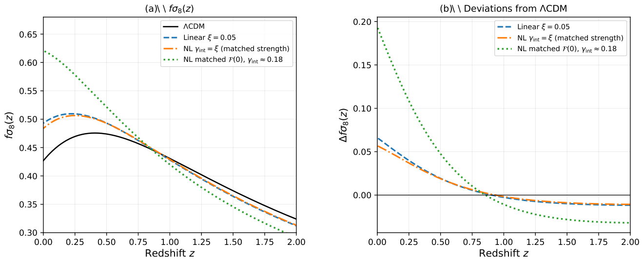
Figure 4.
Two limiting cases of . Panel (a): for deviations whose perturbation-level structure is uniform across observable scales ( gravity, IDE), reduces to a single function of redshift, indexed equivalently by or by . Panel (b): for deviations whose effective gravitational coupling is scale-dependent ( gravity), inherits k-structure through the scalaron’s Compton wavenumber , and the third-vertex test must be satisfied at every observable scale. The inset in the right panel sketches the transition of across from the super-Compton value to the sub-Compton value ; the lower row shows the resulting signature in as a family of curves rather than a single deviation. The dashed grey reference is CDM in both panels.
Figure 4.
Two limiting cases of . Panel (a): for deviations whose perturbation-level structure is uniform across observable scales ( gravity, IDE), reduces to a single function of redshift, indexed equivalently by or by . Panel (b): for deviations whose effective gravitational coupling is scale-dependent ( gravity), inherits k-structure through the scalaron’s Compton wavenumber , and the third-vertex test must be satisfied at every observable scale. The inset in the right panel sketches the transition of across from the super-Compton value to the sub-Compton value ; the lower row shows the resulting signature in as a family of curves rather than a single deviation. The dashed grey reference is CDM in both panels.
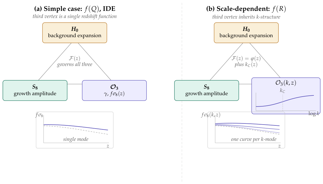
Disclaimer/Publisher’s Note: The statements, opinions and data contained in all publications are solely those of the individual author(s) and contributor(s) and not of MDPI and/or the editor(s). MDPI and/or the editor(s) disclaim responsibility for any injury to people or property resulting from any ideas, methods, instructions or products referred to in the content. |
© 2026 by the authors. Licensee MDPI, Basel, Switzerland. This article is an open access article distributed under the terms and conditions of the Creative Commons Attribution (CC BY) license (http://creativecommons.org/licenses/by/4.0/).
Copyright: This open access article is published under a Creative Commons CC BY 4.0 license, which permit the free download, distribution, and reuse, provided that the author and preprint are cited in any reuse.