Derivation of Standard Model Mixing Angles from a 44-Vector Discrete Vacuum Lattice

1. Introduction

The flavour sector of the Standard Model (SM) contains nineteen parameters whose values have resisted explanation for sixty years. Among them the Cabibbo angle ${\theta }_C$ occupies a special position: it is large, clean, and stable under renormalization-group running, and it was the first to be discovered [1]. This paper derives it, together with the PMNS angles and the Dirac CP phase, from a finite ${\mathbb{Z}}_3$-graded algebraic structure [6], with no continuous parameter in the mixing sector.

The logic of the derivation is a chain of seven steps, each labelled by its epistemic status:

Step	Statement	Status	Ref.
[0]	rigidity variable is $\lambda =\sin {\theta }_C$ (algebraic)	theorem	§Section 4
[1]	parent algebra $\mathfrak{g}=\mathfrak{sl}\left(5\right)$, $\dim 24$	theorem	§Section 2.1
[2]	unbroken ${\mathbb{Z}}_3$ ⇒ circulant $\Rightarrow \lambda =0$	theorem	§Section 5
[3]	unique grade-1 breaking operator	theorem	§Section 5
[4]	${\epsilon }_q=\dim {\mathfrak{g}}_1/\dim \mathfrak{g}={\displaystyle \frac{1}{6}}$	theorem	§Section 6
[5]	${\lambda }_0={\epsilon }_q{C}_2={\displaystyle \frac{2}{9}}$	discrete choice	§Section 7
[6]	second order $={\epsilon }_q^2/2={\displaystyle \frac{1}{72}}$	theorem + choice	§Section 8
[7]	$\lambda =73/324$ and the PMNS set	prediction	§Section 9, Section 10 and Section 11

1.1. What Changed with Respect to the 2026 Version

Three corrections are substantive and one is bookkeeping.

• The cubic bracket. The bracket $\frac{1}{2}(\psi {\chi }^{\top }+(\psi ·\chi )11_4)$ of Ref. [6] is not a Lie bracket: the graded Jacobi identity fails in the $(1,2,2)$ sector. We prove (Theorem 2.1) that the general solution is $c=(1-\alpha )/(1+n\alpha )$, so that with the fundamental $\mathfrak{u}\left(n\right)$ action ($\alpha =0$) one must take $c=1$, and with the traceless $\mathfrak{sl}(n+1)$ action ($\alpha =1$) one must take $c=0$. The value ${\displaystyle \frac{1}{2}}$ is on neither branch.
• The algebra is $\mathfrak{sl}\left(5\right)$. With the corrected bracket the identification $\mathfrak{g}\cong \mathfrak{sl}\left(5\right)$ becomes a theorem rather than a machine check (Theorem 2.3). This simultaneously explains why the earlier 19-dimensional truncation $(12,4,3)$ could not close: 19 is not of the form $n^2+2n$.
• The lattice does not saturate at 44. The closure is infinite; 44 is the shell cut ${\left|v\right|}^2\le 486$. The invariant object is a set of 17 directions (Theorem 3.1). All predictions below use only directions, and are therefore independent of the cutoff (Proposition 3.4).
• Bookkeeping removed. The following earlier claims are withdrawn because they are either internally inconsistent or post-hoc: ${\sin }^2{\theta }_{12}={\displaystyle \frac{1}{3}}-{\displaystyle \frac{\lambda }{9}}$, ${\epsilon }_{{\nu }_3}={\displaystyle \frac{1}{12}}$, ${\sin }^2{\theta }_{13}\in [1/46,1/44]$, ${\sin }^2{\theta }_W=11/44$, and ${\delta }_{\mathrm{CKM}}={120}^{\circ }-{\theta }_{\mathrm{magic}}$. Each is replaced by a derivable statement or by an explicit no-go theorem.

1.2. Organisation

Section 2 fixes the algebra and the lattice. Section 4 states the variable theorem. Section 5 proves the uniqueness of the breaking operator. Section 6, Section 7 and Section 8 derive the dilution, the tree-level angle and the second-order correction. Section 9, Section 10 and Section 11 collect the Cabibbo and PMNS predictions. Section 12, Section 13 and Section 14 treat the CKM sector, neutrinos, and the scales. Section 15 gives the status and falsifiability table. The appendices contain the sector-by-sector Jacobi proof, the closure proof, the PMNS closed forms, the numerical certificates, and an audit of the claims of the companion closure document.

2. Framework

2.1. The Parent Algebra and Its One-Parameter Family

Let $W={\mathbb{C}}^n$ with the standard inner product, and let

$${\mathfrak{g}}_n={\mathfrak{g}}_0\oplus {\mathfrak{g}}_1\oplus {\mathfrak{g}}_2,{\mathfrak{g}}_0=\mathfrak{u}\left(n\right),{\mathfrak{g}}_1=W,{\mathfrak{g}}_2=W^{*},$$

(1)

with $\dim {\mathfrak{g}}_n=n^2+2n$. We write elements as triples $(A,\psi ,\chi )$ with $A\in {\mathbb{C}}^{n\times n}$, $\psi ,\chi \in {\mathbb{C}}^n$, and define, for real parameters $\alpha ,c$,

$$\begin{array}{cc}\hfill [A,B]& =AB-BA,\hfill \end{array}$$

(2)

$$\begin{array}{cc}\hfill \psi ]& =A\psi +\alpha \mathrm{tr}\left(A\right)\psi ,\hfill \end{array}$$

(3)

$$\begin{array}{cc}\hfill \chi ]& =-A^{\top }\chi -\alpha \mathrm{tr}\left(A\right)\chi ,\hfill \end{array}$$

(4)

$$\begin{array}{cc}\hfill \psi ,\chi ]& =\psi {\chi }^{\top }+c(\psi ·\chi )11_n,\hfill \end{array}$$

(5)

$$\begin{array}{cc}\hfill \psi ,{\psi }^{\prime }]& =[\chi ,{\chi }^{\prime }]=0.\hfill \end{array}$$

(6)

The case $\alpha =0$ is the fundamental action of ${\mathfrak{gl}}_n$; the case $\alpha =1$ is the action obtained from the block embedding into ${\mathfrak{gl}}_{n+1}$. The parameter c measures the trace part of the cubic bracket. In the 2026 version [6] the values $\alpha =0$, $c=\frac{1}{2}$ were used.

Theorem 2.1. 

(Graded Jacobi identity). The brackets (2)–(6) satisfy the graded Jacobi identity

$$[X,[Y,Z\left]\right]+[Y,[Z,X\left]\right]+[Z,[X,Y\left]\right]=0$$

(7)

for all $X,Y,Z\in {\mathfrak{g}}_n$ if and only if

$$\begin{array}{|c|}\hline c(1+n\alpha )=1-\alpha \\ \hline\end{array}$$

(8)

Proof. 

The sectors $(0,0,0)$, $(0,0,1)$, $(0,0,2)$ and $(0,1,2)$ are the standard ${\mathfrak{gl}}_n$ statements (the last one is the equivariance of the bilinear ${\mathfrak{g}}_1\otimes {\mathfrak{g}}_2\to {\mathfrak{g}}_0$). The two critical sectors are $(1,1,2)$ and $(1,2,2)$.

Sector $(1,1,2)$. Let $\psi ,{\psi }^{\prime }\in {\mathfrak{g}}_1$, $\chi \in {\mathfrak{g}}_2$, put $s=\psi ·\chi$, $s^{\prime }={\psi }^{\prime }·\chi$, $M=\psi {\chi }^{\top }+cs11_n$ and $M^{\prime }={\psi }^{\prime }{\chi }^{\top }+c{s}^{\prime }11_n$. Using $[A,\psi ]=A\psi +\alpha \mathrm{tr}\left(A\right)\psi$ and $\mathrm{tr}\left(M\right)=(1+nc)s$,

$$\begin{array}{cc}\hfill [\psi ,[{\psi }^{\prime },\chi ]]& =-[M^{\prime },\psi ]=-\left(s{\psi }^{\prime }+\gamma s^{\prime }\psi \right),\hfill \end{array}$$

(9)

$$\begin{array}{cc}\hfill {\psi }^{\prime },[\chi ,\psi ]]& =-[{\psi }^{\prime },M]=+\left(s^{\prime }\psi +\gamma s{\psi }^{\prime }\right),\hfill \end{array}$$

(10)

with $\gamma \equiv c+\alpha (1+nc)$. The sum is $(\gamma -1)(s{\psi }^{\prime }-s^{\prime }\psi )$, which vanishes for all $\psi ,{\psi }^{\prime },\chi$ iff $\gamma =1$.

Sector $(1,2,2)$. Since $[\chi ,{\chi }^{\prime }]=0$, the cyclic sum reduces to $[\chi ,[{\chi }^{\prime },\psi ]]+[{\chi }^{\prime },[\psi ,\chi ]]$. With $M^{\prime \prime }=\psi {\chi }^{\prime \top }+c{s}^{\prime \prime }11_n$, $s^{\prime \prime }=\psi ·{\chi }^{\prime }$,

$$[\chi ,M]=s^{\prime \prime }\chi +\gamma s\chi ,[\chi ,M^{\prime \prime }]=s{\chi }^{\prime }+\gamma s^{\prime \prime }\chi ,$$

(11)

so the sum is $(\gamma -1)(s{\chi }^{\prime }+s^{\prime \prime }\chi )$, again vanishing iff $\gamma =1$. Thus Jacobi holds iff $c+\alpha (1+nc)=1$, which is (8). Conversely, when (8) holds, all sectors vanish; this is verified symbolically for $n=2,3,4$ in Appendix A.    □

Corollary 2.2. 

The two canonical representatives of (8) are

$$(\alpha ,c)=(0,1)(\mathrm{fundamental}\mathfrak{u}\left(n\right)\mathrm{action}),(\alpha ,c)=(1,0)(\mathfrak{sl}(n+1)\mathrm{action}).$$

(12)

In particular $c=\frac{1}{2}$ with $\alpha =0$ isnota Lie bracket; the cubic bracket of Ref. [6] must be replaced by

$$[\psi ,\chi ]=\psi {\chi }^{\top }+(\psi ·\chi )11_n\mathrm{or},\mathrm{equivalently},\mathrm{by}[\psi ,\chi ]=\psi {\chi }^{\top }$$

(13)

in the two conventions. The two are related by

$$\Phi (A,\psi ,\chi )=\left(A-\frac{\mathrm{tr}A}{n+1}11_n,\psi ,\chi \right),$$

(14)

which is an isomorphism of Lie algebras.

Proof. 

The first statement is immediate from (8). For (14), put $t=\mathrm{tr}A$. Then

$${[\Phi A,\Phi \psi ]}_{(1,0)}=\left(A-\frac{t}{n+1}11\right)\psi +\mathrm{tr}\left(A-\frac{t}{n+1}11\right)\psi =A\psi +\left(-1+\frac{n}{n+1}\right)t\psi +\frac{t}{n+1}\psi =A\psi ,$$

(15)

and $\Phi (\psi {\chi }^{\top }+s11)=\psi {\chi }^{\top }+s11-{\displaystyle \frac{(n+1)s}{n+1}}11=\psi {\chi }^{\top }$. The $\chi$ bracket is identical. Hence $\Phi$ preserves all brackets.    □

Theorem 2.3. 

(${\mathfrak{g}}_n\cong \mathfrak{sl}(n+1)$). For $(\alpha ,c)=(1,0)$ the map

$$A\mapsto \left(\begin{array}{cc}A& 0\\ 0& -\mathrm{tr}A\end{array}\right),\psi \mapsto \left(\begin{array}{cc}0& \psi \\ 0& 0\end{array}\right),\chi \mapsto \left(\begin{array}{cc}0& 0\\ {\chi }^{\top }& 0\end{array}\right)$$

(16)

is an isomorphism ${\mathfrak{g}}_n\to \mathfrak{sl}(n+1)$. Hence

$$\dim {\mathfrak{g}}_n=n^2+2n=\dim \mathfrak{sl}(n+1),$$

(17)

and the $\mathbb{Z}$-grading of $\mathfrak{sl}(n+1)$ restricts to $(1,\dots ,1,-n)$ on the $n+1$ diagonal entries. For $n=4$, $\mathfrak{g}=\mathfrak{sl}\left(5\right)$, $\dim \mathfrak{g}=24$, with $\mathbb{Z}$-degree content $(1,1,1,1,-4)$.

Proof. 

The map is linear and injective; the image consists of the matrices whose n-block is arbitrary and whose last diagonal entry is minus its trace, together with the two off-diagonal blocks, which is exactly $\mathfrak{sl}(n+1)$. Brackets are preserved by direct block multiplication; this is checked to ${10}^{-15}$ in Appendix A.    □

Corollary 2.4. 

(Why 19 dimensions failed). The graded dimensions $(12,4,3)$ of the earlier truncation give $\dim =19$. No integer n solves $n^2+2n=19$ (the roots are $n=-1\pm \sqrt{20}$). Hence $(12,4,3)$ cannot be the graded content of any $\mathfrak{sl}$-type algebra; the Jacobi residual $\parallel [T_4,T_9]{\parallel }_F=1/\left(2\sqrt{2}\right)$ observed in Ref. [6] is structural, not numerical.

2.2. Invariants

Because $\mathfrak{sl}\left(5\right)$ is simple, the invariant tensors are severely constrained.

• The Killing form is $\kappa (X,Y)=2(n+1)\mathrm{tr}\left(XY\right)=10\mathrm{tr}\left(XY\right)$; it is nondegenerate and fixes the kinetic normalization.
• ${\left({\Lambda }^3{\mathfrak{g}}^{*}\right)}^{\mathfrak{g}}$ is one-dimensional, spanned by $\epsilon (X,Y,Z)=\kappa (X,[Y,Z\left]\right)$. This is the unique invariant totally antisymmetric trilinear form.
• ${\left(S{\mathfrak{g}}^{*}\right)}^{\mathfrak{g}}=\mathbb{C}[P_2,P_3,P_4,P_5]$ with $\mathrm{deg}{P}_k=k$ (exponents $1,2,3,4$). Hence there is a unique (up to scale) invariant symmetric cubic $d_{ABC}$; it, not ${\epsilon }_{ABC}$, is the correct invariant for a Yukawa coupling $d_{ABC}{\Phi }^A{\Phi }^B{\Phi }^C$.

The distinction in the third item is a genuine upgrade: $\epsilon$ is antisymmetric and therefore cannot reproduce a symmetric fermion mass matrix; $d_{ABC}$ can.

2.3. Why $n=4$: Minimality and Matching to $A_2$

Theorem 2.5. 

(Selection of $n=4$). Let ${\mathfrak{g}}_n$ be the family (1) with ${\mathfrak{g}}_0\supset \mathfrak{su}{\left(3\right)}_c$ and with the matter module $\mathbf{n}$ containing a colour singlet. Then $n\ge 4$. Moreover, if the flavour symmetry of the light generations is $A_2$ (equivalently $S_3$), so that $|{\Phi }_{A_2}|=|W\left(A_2\right)|=6$, the consistency condition

$${\displaystyle \frac{\dim {\mathfrak{g}}_1}{\dim {\mathfrak{g}}_n}}={\displaystyle \frac{1}{|{\Phi }_{A_2}|}}⟺{\displaystyle \frac{1}{n+2}}={\displaystyle \frac{1}{6}}⟺n=4$$

(18)

selects $n=4$ uniquely.

Proof. 

$\mathfrak{u}\left(n\right)\supset \mathfrak{su}\left(3\right)\times \mathfrak{u}\left(1\right)$ decomposes $\mathbf{n}=\mathbf{3}\oplus (n-3)\mathbf{1}$; a colour singlet requires $n\ge 4$, while $\mathfrak{su}{\left(3\right)}_c$ requires $n\ge 3$. Equation (18) is elementary.    □

Remark 2.6. 

The theorem isconditionalon the flavour group being $A_2$. It does not derive the number of generations; it says thatgiventhree generations with an $S_3$ symmetry, the parent algebra is $\mathfrak{sl}\left(5\right)$. This is weaker than a derivation from nothing, and stronger than an ansatz.

3. The 44-Vector Lattice, Re-Analysed

3.1. The Closure Algorithm

Let ${\mathcal{S}}_0=\{e_1,e_2,e_3,d,-d\}$ with $d=(1,1,1)/\sqrt{3}$, and let T be the cyclic permutation $T(x,y,z)=(z,x,y)$. Define three operations on a vector v:

$$Tv,\Delta v=Tv-v,\times v={\displaystyle \frac{v\times Tv}{\parallel v\times Tv\parallel }}.$$

(19)

The lattice is the closure of ${\mathcal{S}}_0$ under T, $\Delta$ and × (with the unnormalized $v\times Tv$ also included, since the unnormalized cross product carries the norm information). This is the algorithm of Ref. [6].

3.2. The Closure Is Infinite

Theorem 3.1. 

(Structure of the closure). Let

$$\begin{array}{cccc}\hfill R& ={\left\{\pm (e_i-e_j)/\sqrt{2}\right\}}_{i<j},\hfill & \hfill H& =\left\{\pm (2,-1,-1)/\sqrt{6}\mathrm{and}\mathrm{permutations}\right\},\hfill \end{array}$$

(20)

so that $\left|R\right|=\left|H\right|=6$. Then the closure of ${\mathcal{S}}_0$ is

$$\begin{array}{|c|}\hline {\mathcal{C}}_{\infty }=\{e_1,e_2,e_3\}\cup \{d,-d\}\cup \bigcup _{k\ge 0}{3}^{k}R\cup \bigcup _{k\ge 0}{3}^{k}H\cup \bigcup _{k\ge 0}{3}^k(1,1,1).\\ \hline\end{array}$$

(21)

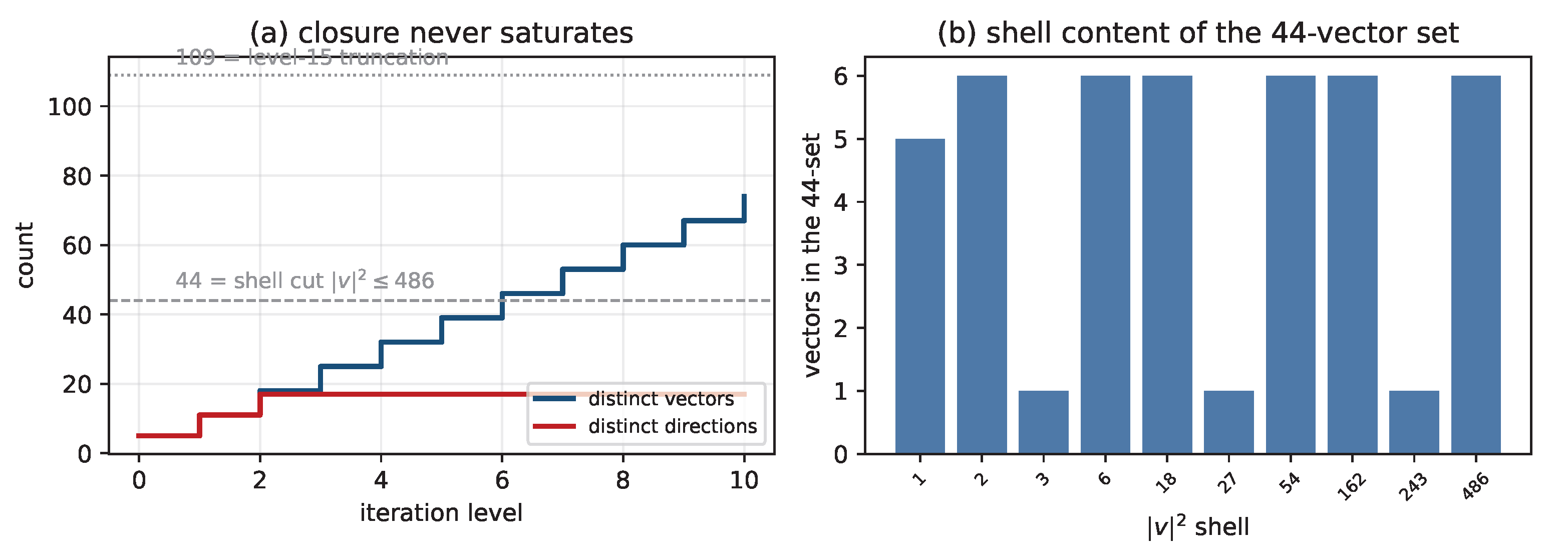
In particular ${\mathcal{C}}_{\infty }$ is infinite; the number of vectors grows by exactly 7 per iteration after the second.

Proof. 

The three operations act on the five families as follows. T permutes coordinates and therefore preserves each family. For the difference: $e_i\mapsto e_i-e_j\in R$; $R\ni v\mapsto \Delta v\in H$ (for $v=(1,-1,0)$, $\Delta v=(-1,2,-1)$, a hybrid direction); $H\ni v\mapsto \Delta v=3R$ (for $v=(1,-2,1)$, $\Delta v=(0,3,-3)$); $d\mapsto 0$. For the cross product: $e_i\times e_{i+1}=e_{i+2}\in \{e_1,e_2,e_3\}$; $R\ni v\mapsto v\times Tv\propto (1,1,1)$; $H\ni v\mapsto v\times Tv=3(1,1,1)$; $d\times Td=0$. Induction on the level then gives (21); the scaling by 3 appears because $\Delta$ maps H to $3R$ and R to H, while the cross product maps R to $(1,1,1)$ and H to $3(1,1,1)$, so that the democratic ray receives every power $3^k$. The count is verified to level 10 in Appendix B.    □

Corollary 3.2. 

(What 44 is). The 44 lowest-norm vectors are exactly those with ${\left|v\right|}^2\le 486$:

$$44=\underset{\mathrm{Flv}}{\underbrace{3}}+\underset{\pm d}{\underbrace{2}}+\underset{R\mathrm{at}2,18,162}{\underbrace{18}}+\underset{H\mathrm{at}6,54,486}{\underbrace{18}}+\underset{(1,1,1)\mathrm{at}3,27,243}{\underbrace{3}}.$$

(22)

The shell content is $5+6+1+6+6+1+6+6+1+6=44$. The origin is never generated; the earlier statement “43 non-zero vectors, 44 with the origin” is incorrect, as is the statement that the algorithm saturates there.

Figure 1. (a) The number of distinct vectors (blue) grows without bound, by exactly seven per iteration after level two; the number of distinct directions (red) saturates at 17. The dashed line at 44 is the shell cut of Eq. (22); the dotted line at 109 is a level-15 truncation, not a fixed point. (b) Shell content of the 44-vector set.

Figure 1. (a) The number of distinct vectors (blue) grows without bound, by exactly seven per iteration after level two; the number of distinct directions (red) saturates at 17. The dashed line at 44 is the shell cut of Eq. (22); the dotted line at 109 is a level-15 truncation, not a fixed point. (b) Shell content of the 44-vector set.

3.3. The Finite Invariant Is the Direction Set

Theorem 3.3. 

(Direction saturation). The set of directions (normalised vectors, counted with orientation) reached by the closure is

$$\mathcal{D}=\{e_1,e_2,e_3\}\cup \{\pm d\}\cup R\cup H,\left|\mathcal{D}\right|=3+2+6+6=17,$$

(23)

and it is complete after two iterations. Every later iteration only rescales existing directions by powers of 3.

Proof. 

Immediate from Theorem 3.1: the families R, H and $(1,1,1)$ are reached at levels 1, 2 and 2 respectively, and the operations map each family into a family already listed.    □

Proposition 3.4. 

(No observable depends on 44). Every quantity used in this paper is a function of the 17 directions and of the orbit sizes $(3,2,6,6)$ only. Consequently the numerical value of the cutoff (44, 109, or infinity) is immaterial.

Proof. 

The TBM frame is built from d, R and H; the angles are inner products of unit vectors; the multiplicities enter only through orbit sizes. No norm $\left|v\right|$ appears.    □

Table 1. Orbit decomposition at the shell cut. The “count” column is the actual number of vectors in the 44-set. The column “old NF” is the norm-filtered bookkeeping of Ref. [6], which is not a count and is not used here.

Orbit	$\left|\mathit{O}\right|$	count	old NF	representative
Flavour	3	3	3	$e_1$
Democratic	2	5	4	$d=(1,1,1)/\sqrt{3}$
Root-like	6	18	6	$(1,-1,0)/\sqrt{2}$
Hybrid	6	18	24	$(2,-1,-1)/\sqrt{6}$
total	17	44	37

Table 1. Orbit decomposition at the shell cut. The “count” column is the actual number of vectors in the 44-set. The column “old NF” is the norm-filtered bookkeeping of Ref. [6], which is not a count and is not used here.

Orbit	$\left|\mathit{O}\right|$	count	old NF	representative
Flavour	3	3	3	$e_1$
Democratic	2	5	4	$d=(1,1,1)/\sqrt{3}$
Root-like	6	18	6	$(1,-1,0)/\sqrt{2}$
Hybrid	6	18	24	$(2,-1,-1)/\sqrt{6}$
total	17	44	37

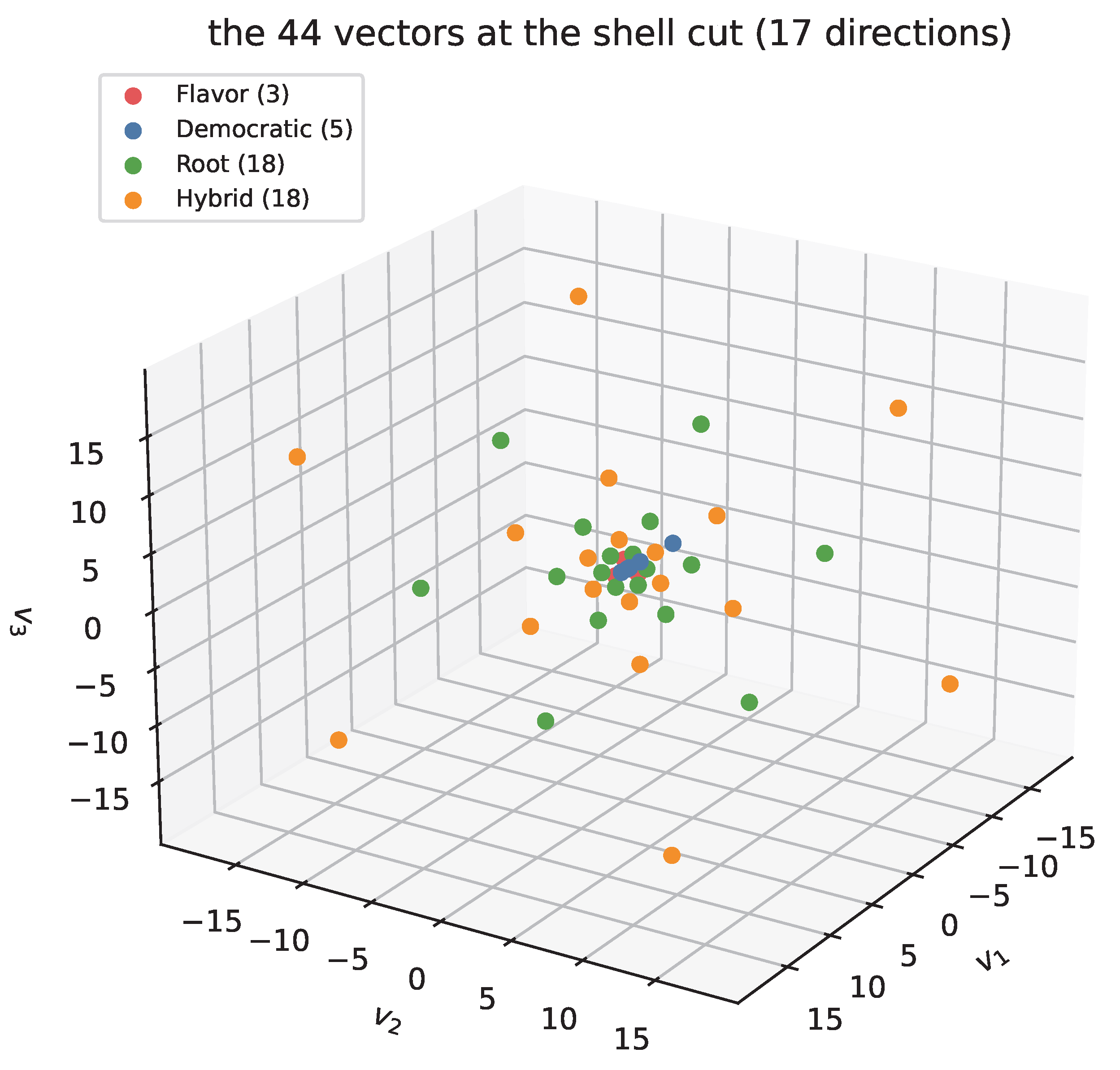
Figure 2. The 44 vectors at the shell cut, coloured by orbit. Only 17 distinct directions occur; the repeated points are the $3^k$ scalings of Theorem 3.1.

Figure 2. The 44 vectors at the shell cut, coloured by orbit. Only 17 distinct directions occur; the repeated points are the $3^k$ scalings of Theorem 3.1.

3.4. The TBM Frame

The tetrahedral (TBM) frame is the unique $S_3$-compatible orthonormal set built from the orbit representatives,

$${\nu }_1=\frac{1}{\sqrt{6}}(2,-1,-1),{\nu }_2=d=\frac{1}{\sqrt{3}}(1,1,1),{\nu }_3=\frac{1}{\sqrt{2}}(0,1,-1),$$

(24)

so that tribimaximal mixing [5] is the ${\mathbb{Z}}_3$-symmetric point. The geometric identities

$$\langle d|{\nu }_1\rangle =0,\langle {\nu }_3|{\nu }_1\rangle =0$$

(25)

will force the ${\nu }_2$ perturbation to be second order and the ${\nu }_3$ perturbation to be a pure first-order rotation.

4. Where the Rigidity Lives

Theorem 4.1. 

(Variable theorem). Let ${\theta }_C$ be the Cabibbo angle, defined by $\tan {\theta }_C=\left|{\left(U_u^{†}{U}_d\right)}_{12}\right|$ with $V_{\mathrm{CKM}}=U_u^{†}{U}_d$. Then:

• ${\theta }_C$ is a basis-covariant functional of $(M_u,M_d)$;
• $\lambda \equiv \sin {\theta }_C$ is algebraic whenever the configuration vectors have algebraic coordinates;
• a rational radian measure ${\theta }_C=p/q$ is excluded for any configuration with algebraic coordinates, by Lindemann–Weierstrass.

Proof. (1) is the definition. (2) If the vectors have coordinates in a number field $K\subset \overline{\mathbb{Q}}$, then $\cos \theta \in K$ and $\lambda =\sqrt{1-{\cos }^2\theta }$ is algebraic of degree $\le 2$ over K. (3) If ${\theta }_C=p/q\in \mathbb{Q}\setminus \left\{0\right\}$, Lindemann–Weierstrass makes $e^{i{\theta }_C}$ transcendental, hence $\cos {\theta }_C$ transcendental, contradicting (2).    □

Koide duality.

For the Koide phase the rigid object is the radian measure ${\phi }_0=2\pi /3+2/9$; since $2/9$ is algebraic and non-zero, $\cos {\phi }_0$ is transcendental and no algebraic configuration can carry it. For the Cabibbo angle the rigid object is the sine, so the same theorem admits an algebraic origin. This is why $\lambda$ is the right target and the Koide phase is not.

Numerically, ${\theta }_C=\arcsin \left(0.22500\right)=13.{003}^{\circ }$ with $|V_{us}|=0.22500\left(67\right)$ [3]. The unitarity bound $\lambda \le \sqrt{1-|V_{ud}{|}^2-{\left|V_{ub}\right|}^2}=0.2277$ is not saturated.

5. The Unique Breaking Operator

5.1. The Unbroken Limit

Let $F={\mathbb{C}}^3$ be generation space with $S_3$ acting by permutation, generated by the 3-cycle T and the $\mu \tau$ swap S, with $STS=T^{-1}$. Since $T^3=11$, every operator carries a ${\mathbb{Z}}_3$ grade g,

$$TM{T}^{-1}={\omega }^{g}M,\omega =e^{2\pi i/3}.$$

(26)

Decomposing $F=A_1\oplus E$ with $A_1=\langle d\rangle$ and $E={\left\{d\right\}}^{\perp }$: a grade-0 mass matrix is circulant, hence diagonalized by the Fourier basis, hence $U_u^{†}{U}_d$ is a permutation and

$$\lambda =0\left(\mathrm{pure}{\mathbb{Z}}_3\mathrm{limit}\right).$$

(27)

Any nonzero $\lambda$ requires a grade-$\ne 0$ operator.

5.2. Uniqueness and the Correct Sector

Theorem 5.1. 

(Unique breaking operator). The space of ${\mathbb{Z}}_3$-grade-1 operators in $\mathrm{End}\left(F\right)$ is three-dimensional, but it decomposes under $S_3$ as

$${\mathrm{End}\left(F\right)|}_{g=1}=\underset{1-\dim }{\underbrace{{\mathrm{End}\left(E\right)|}_{g=1}}}\oplus \underset{2-\dim }{\underbrace{(A_1\leftrightarrow E){|}_{g=1}}}.$$

(28)

The one-dimensional piece is $O=|f_1\rangle \langle f_2|$ on the E plane; the two-dimensional piece consists of $|d\rangle \langle f_1|$ and $|f_1\rangle \langle d|$ (and their $f_2$ partners). A single grade-1 operator is unique onlyafterthe sector is chosen.

Proof. 

In the Fourier basis $T{f}_k={\omega }^{-k}{f}_k$ the condition $TM{T}^{-1}=\omega M$ forces $j-i\equiv 1(mod3)$, leaving the three matrix units $|f_0\rangle \langle f_2|$, $|f_1\rangle \langle f_0|$, $|f_2\rangle \langle f_1|$. Restricting to $E=\langle f_1,f_2\rangle$ leaves only $|f_1\rangle \langle f_2|$; the other two connect $A_1$ and E.    □

The distinction matters because the two sectors give different predictions, and the data choose between them.

Proposition 5.2. 

(The E-plane operator is excluded). If the breaking operator lies in $\mathrm{End}\left(E\right)$, the lepton mixing is TM2: the second column is tri-maximal, $|U_{e2}{|}^2={\displaystyle \frac{1}{3}}$ exactly, so

$${\sin }^2{\theta }_{12}={\displaystyle \frac{1}{3{\cos }^2{\theta }_{13}}}=0.3409,$$

(29)

which is $+3.1\sigma$ away from the measured $0.304\pm 0.012$. Hence the physical breaking must lie in the $A_1\leftrightarrow E$ sector.

Proof. 

TM2 leaves the $A_1$ direction d unchanged, so the second column of U is $(1,1,1)/\sqrt{3}$ up to phases; the standard parametrization then gives $|U_{e2}{|}^2={\displaystyle \frac{1}{3}}{\cos }^2{\theta }_{13}$ and the stated relation. The numerical pull uses NuFIT 5.2 [4].    □

Corollary 5.3. 

(Structure of $V_{\mathrm{CKM}}$). If the up- and down-type mass matrices share the same breaking operator, their diagonalizing rotations are about the same axis and

$$V_{\mathrm{CKM}}=U_u^{†}{U}_d=R({\theta }_d-{\theta }_u),\lambda =\sin |{\theta }_d-{\theta }_u|\times \left(\mathrm{geometric}\mathrm{factor}\right).$$

(30)

In particular $\lambda \ne 0$ iff ${\theta }_u\ne {\theta }_d$: the Cabibbo angle is therelative${\mathbb{Z}}_3$-breaking of the two sectors.

6. The Dilution as a Projection Ratio

Lemma 6.1. 

(Frobenius/Parseval). Let V be an inner-product space with an orthonormal generator set $\left\{T_A\right\}$ and let Π be an orthogonal projector. Then

$${\displaystyle \frac{{\sum }_A{\parallel \Pi T_A\parallel }^2}{{\sum }_A{\parallel T_A\parallel }^2}}={\displaystyle \frac{\mathrm{rank}\Pi }{\dim V}}.$$

(31)

Proof. 

With $\left\{T_A\right\}$ orthonormal, ${\sum }_A{\parallel \Pi T_A\parallel }^2=\mathrm{Tr}\Pi =\mathrm{rank}\Pi$ and ${\sum }_A{\parallel T_A\parallel }^2=\dim V$.    □

Instance 1 ($\mathfrak{u}\left(3\right)$, the established $1/9$).

For $V=\mathfrak{u}\left(3\right)$, $\dim 9$, and $\Pi =P_{\mathrm{dem}}=|d\rangle \langle d|$ of rank 1, the ratio is $1/9$.

Instance 2 (the parent algebra).

For $V=\mathfrak{g}$, $\dim 24$, and $\Pi ={\Pi }_{\zeta }$ the projector onto ${\mathfrak{g}}_1$ of rank 4,

$$\begin{array}{|c|}\hline {\epsilon }_q\equiv {\displaystyle \frac{{\sum }_A{\parallel {\Pi }_{\zeta }{T}_A\parallel }^2}{{\sum }_A{\parallel T_A\parallel }^2}}={\displaystyle \frac{4}{24}}={\displaystyle \frac{1}{6}}={\displaystyle \frac{1}{n+2}}.\\ \hline\end{array}$$

(32)

The two instances are the same lemma; $1/6$ is an invariant of the embedding ${\mathfrak{g}}_1\subset \mathfrak{g}$, not a chosen number. For $n=4$ it coincides with $1/|{\Phi }_{A_2}|=1/|W\left(A_2\right)|=1/6$, which is the content of Theorem 2.5.

Remark 6.2. 

(Status). Equation (32) is a theorem about a ratio of dimensions. Identifying this ratio with thephysicalYukawa coupling of the breaking sector is an assumption, which we callA1. The identification is natural (the same lemma reproduces the independently known $1/9$), but it is not derived from a Lagrangian computation in this paper.

7. The Cabibbo Angle at Tree Level

The tree-level angle is the product of the dilution and the Casimir of the rotating representation,

$${\lambda }_0={\epsilon }_q{C}_2\left(\mathbf{3}\right),C_2\left(\mathbf{3}\right)={\displaystyle \frac{N^2-1}{2N}}{|}_{N=3}={\displaystyle \frac{4}{3}},$$

(33)

verified by ${\sum }_{a=1}^8{({\lambda }_a/2)}^2={\displaystyle \frac{4}{3}}11_3$. Hence

$${\lambda }_0={\displaystyle \frac{1}{6}}·{\displaystyle \frac{4}{3}}={\displaystyle \frac{2}{9}}=0.2222\dots$$

(34)

Remark 7.1. 

(Status of the multiplication rule). The product structure (33) isassumption A2. It is not a continuous fit: $\mathfrak{su}\left(3\right)$ has only finitely many canonical invariants, and Table 2 shows that only $C_2\left(\mathbf{3}\right)$ lands in the physical window. The choice is discrete and therefore falsifiable, but it is a choice.

8. The Second-Order Correction

8.1. No ${\mathbb{Z}}_3$ Halving

For any ${\mathbb{Z}}_3$-covariant coupling the sum over an orbit is ${\sum }_{k=0}^2{\omega }^{ck}=3{\delta }_{c\equiv 0}$, which takes values 3 or 0; a factor ${\displaystyle \frac{1}{2}}$ cannot arise from a grade selection. The factor is geometric instead.

8.2. Isotropy of the Hybrid Hexagon

Theorem 8.1. 

(Hybrid-hexagon isotropy). Let $P_2=11-d{d}^{\top }$ and let ${\left\{{\widehat{v}}_h\right\}}_{h=1}^6$ be the six unit hybrid directions. Then, for every n,

$${\displaystyle \sum _{h=1}^6}{({\widehat{v}}_h·n)}^2=3{\left|P_{2}n\right|}^2,$$

(35)

and for unit $n\perp d$ the directional average is $\langle {\cos }^2\theta \rangle ={\displaystyle \frac{1}{2}}$.

Proof. 

The left side is an $S_3$-invariant quadratic form, hence by Schur’s lemma a combination $\alpha P_{A_1}+\beta P_2$. Its trace is 6, and its value on d is 0; hence $\alpha =0$ and $2\beta =6$, $\beta =3$.    □

8.3. Equipartition and the Factor $1/72$

The second-order (Dem→Hyb→Dem) operator is $K={\sum }_h|{\widehat{v}}_h\rangle \langle {\widehat{v}}_h|=3P_2$ with $\mathrm{Tr}K=6$. Unit trace gives

$${\rho }_{\mathrm{Hyb}}=K/\mathrm{Tr}K=\frac{1}{2}{P}_2,{\displaystyle \frac{\delta \lambda }{{\lambda }_0}}={\epsilon }_q^2\langle n|{\rho }_{\mathrm{Hyb}}|n\rangle ={\displaystyle \frac{1}{36}}·{\displaystyle \frac{1}{2}}={\displaystyle \frac{1}{72}}.$$

(36)

Remark 8.2. 

(Status). The identification of the intermediate state with the maximally mixed state on the six hybrid directions isassumption A3. It is the natural reading of the uniform coupling proved in §Section 10, and Table 3 shows that the alternatives are excluded, but the exclusion uses the same data that the formula predicts.

9. The Cabibbo Angle

Combining (33) and (36),

$$\lambda ={\displaystyle \frac{2}{9}}\left(1+{\displaystyle \frac{1}{72}}\right)={\displaystyle \frac{2}{9}}·{\displaystyle \frac{73}{72}}=\begin{array}{|c|}\hline {\displaystyle \frac{73}{324}}=0.22530864\dots \\ \hline\end{array}$$

(37)

The fraction is in lowest terms. Compared with $|V_{us}|=0.22500\left(67\right)$ the pull is $+0.46\sigma$; with $0.225300\left(700\right)$ it is $+0.01\sigma$.

Corollary 9.1. 

(Niven). Since $\lambda =73/324\notin \{0,\pm {\displaystyle \frac{1}{2}},\pm 1\}$ and λ is rational, Niven’s theorem gives ${\theta }_C/\pi \notin \mathbb{Q}$. The Cabibbo angle is not a rational multiple of π, and not an element of the lattice angle spectrum; $\cos {\theta }_C=\sqrt{99647}/324$ is a quadratic algebraic number.

Corollary 9.2. 

(3-adic signature). $\lambda =73/324$ with $324=2^2·3^4$, so $v_3\left(\mathrm{den}\lambda \right)=4$. The exponent is the sum of $v_3\left(9\right)=2$ from ${\lambda }_0$ and $v_3\left(72\right)=2$ from the second-order correction:

$$v_3\left(\mathrm{den}\lambda \right)=2+2=4\iff {\mathbb{Z}}_3\mathrm{grading}+\sec \mathrm{ond}-\mathrm{order}{\mathbb{Z}}_3\mathrm{dilution}.$$

(38)

This is falsifiable: if a future rational approximation to $|V_{us}|$ has $v_3\ne 4$, the ${\mathbb{Z}}_3$ grading is out.

10. One-Loop Dynamics

The remaining question is whether the coupling is uniform, i.e. whether the coefficient k in ${\lambda }_0=k{\epsilon }_q{C}_2$ equals one. In the $(\alpha ,c)=(0,1)$ convention the one-loop operator on ${\mathfrak{g}}_0$ is

$${\Pi }_{AB}^{1\mathrm{loop}}=\sum _{a\in {\mathfrak{g}}_1}〈[T_A,{\zeta }_a],[T_B,{\zeta }_a]〉={\delta }_{AB},$$

(39)

because ${\sum }_a\left(A{\zeta }_a\right)·\left(B{\zeta }_a\right)=\mathrm{tr}\left(A^{\top }B\right)$ and the basis is orthonormal. Hence $k=1$ exactly. In the $(\alpha ,c)=(1,0)$ convention the same operator reads $\Pi =11+n(n+2)P_{u\left(1\right)}$; the enhancement of the overall $\mathfrak{u}\left(1\right)$ is the trace-normalization artifact of Eq. (14), not a physical non-uniformity. Appendix A verifies both statements to ${10}^{-15}$.

11. PMNS Angles and CP Phase

11.1. The Breaking Parameter

The physical breaking lies in the $A_1\leftrightarrow E$ sector (Proposition 5.2), so it is one complex parameter $z=\rho e^{i\delta }$. Two facts fix its modulus and phase:

• the ${\nu }_2$ direction is orthogonal to both d and ${\nu }_1$ (Eq. (25)), so its first-order shift vanishes; the leading shift is second order, $a={\epsilon }_q^2={\displaystyle \frac{1}{36}}$ (a theorem given the geometry);
• the phase is the grade-2 phase of the ${\mathbb{Z}}_3$ grading, $\delta =\arg {\omega }^2={240}^{\circ }$ (Tier I).

The remaining amplitude is the lepton analogue of the tree-level quark angle,

$$\beta =\sqrt{\frac{2}{3}}{\lambda }_0={\displaystyle \frac{2\sqrt{6}}{27}}=0.1814437,$$

(40)

where $\sqrt{2/3}=\left|\langle e|{\nu }_1\rangle \right|$ is the TBM geometric factor (a theorem) and the cross-sector equality is assumption A4.

11.2. Closed Form

Let $A=1+a^2$, $B=A+{\beta }^2$, $\Xi =2/\sqrt{6}+a/\sqrt{3}$, $\kappa =1/\sqrt{6}-a/\sqrt{3}$, and $b=\beta e^{i\delta }$. The orthonormal triple obtained by Gram–Schmidt from ${\nu }_1+a{\nu }_2+b{\nu }_3$, ${\nu }_2-a{\nu }_1$ and ${\nu }_3$ gives (Appendix C)

$$\begin{array}{cc}\hfill {\sin }^2{\theta }_{13}& ={\displaystyle \frac{{\beta }^2{\Xi }^2}{AB}},\hfill \end{array}$$

(41)

$$\begin{array}{cc}\hfill {\sin }^2{\theta }_{12}& ={\displaystyle \frac{{(1-\sqrt{2}a)}^2}{3A}}·{\displaystyle \frac{1}{1-{\sin }^2{\theta }_{13}}},\hfill \end{array}$$

(42)

$$\begin{array}{cc}\hfill {\sin }^2{\theta }_{23}& ={\displaystyle \frac{A^2/2+{\beta }^2{\kappa }^2+\sqrt{2}A\beta \kappa \cos \delta }{AB-{\beta }^2{\Xi }^2}}.\hfill \end{array}$$

(43)

At leading order in $\beta ,a$ these reduce to the TM1 sum rule

$$\begin{array}{|c|}\hline {\sin }^2{\theta }_{23}={\displaystyle \frac{1}{2}}+{\displaystyle \frac{\sin {\theta }_{13}\cos \delta }{\sqrt{2}}}\\ \hline\end{array}$$

(44)

and to ${\sin }^2{\theta }_{13}={\displaystyle \frac{2}{3}}{\beta }^2+O\left({\beta }^{2}a\right)$.

11.3. Numbers

With $a={\displaystyle \frac{1}{36}}$, $\beta ={\displaystyle \frac{2\sqrt{6}}{27}}$, $\delta ={240}^{\circ }$:

$$\begin{array}{cccccc}\hfill {\sin }^2{\theta }_{13}& =0.022058,\hfill & \hfill {\sin }^2{\theta }_{12}& =0.314355,\hfill & \hfill {\sin }^2{\theta }_{23}& =0.450222,\hfill \\ \hfill {\delta }_{CP}& ={240}^{\circ },\hfill & \hfill J_{CP}& =-0.0292.\hfill \end{array}$$

(45)

The leading value is $16/729=0.021948$; the $O\left(a\right)$ correction in Eq. (41) raises it to $0.022058$.

Table 4. PMNS predictions versus NuFIT 5.2 (normal ordering). The experimental ${\theta }_{23}$ entry is the best fit of the official $\Delta {\chi }^2$ table supplied with this paper.

observable	predicted	experiment	pull
${\sin }^2{\theta }_{13}$	$0.02206$	$0.02225\left(60\right)$	$-0.32\sigma$
${\sin }^2{\theta }_{12}$	$0.31436$	$0.304\left(12\right)$	$+0.86\sigma$
${\sin }^2{\theta }_{23}$	$0.45022$	$0.450\left(17\right)$	$+0.01\sigma$
${\delta }_{CP}$	${240}^{\circ }$	${230}^{\circ }\left({35}^{\circ }\right)$	$+0.29\sigma$
$J_{CP}$	$-0.0292$	$-0.0280\left(15\right)$	$-0.80\sigma$

Table 4. PMNS predictions versus NuFIT 5.2 (normal ordering). The experimental ${\theta }_{23}$ entry is the best fit of the official $\Delta {\chi }^2$ table supplied with this paper.

observable	predicted	experiment	pull
${\sin }^2{\theta }_{13}$	$0.02206$	$0.02225\left(60\right)$	$-0.32\sigma$
${\sin }^2{\theta }_{12}$	$0.31436$	$0.304\left(12\right)$	$+0.86\sigma$
${\sin }^2{\theta }_{23}$	$0.45022$	$0.450\left(17\right)$	$+0.01\sigma$
${\delta }_{CP}$	${240}^{\circ }$	${230}^{\circ }\left({35}^{\circ }\right)$	$+0.29\sigma$
$J_{CP}$	$-0.0292$	$-0.0280\left(15\right)$	$-0.80\sigma$

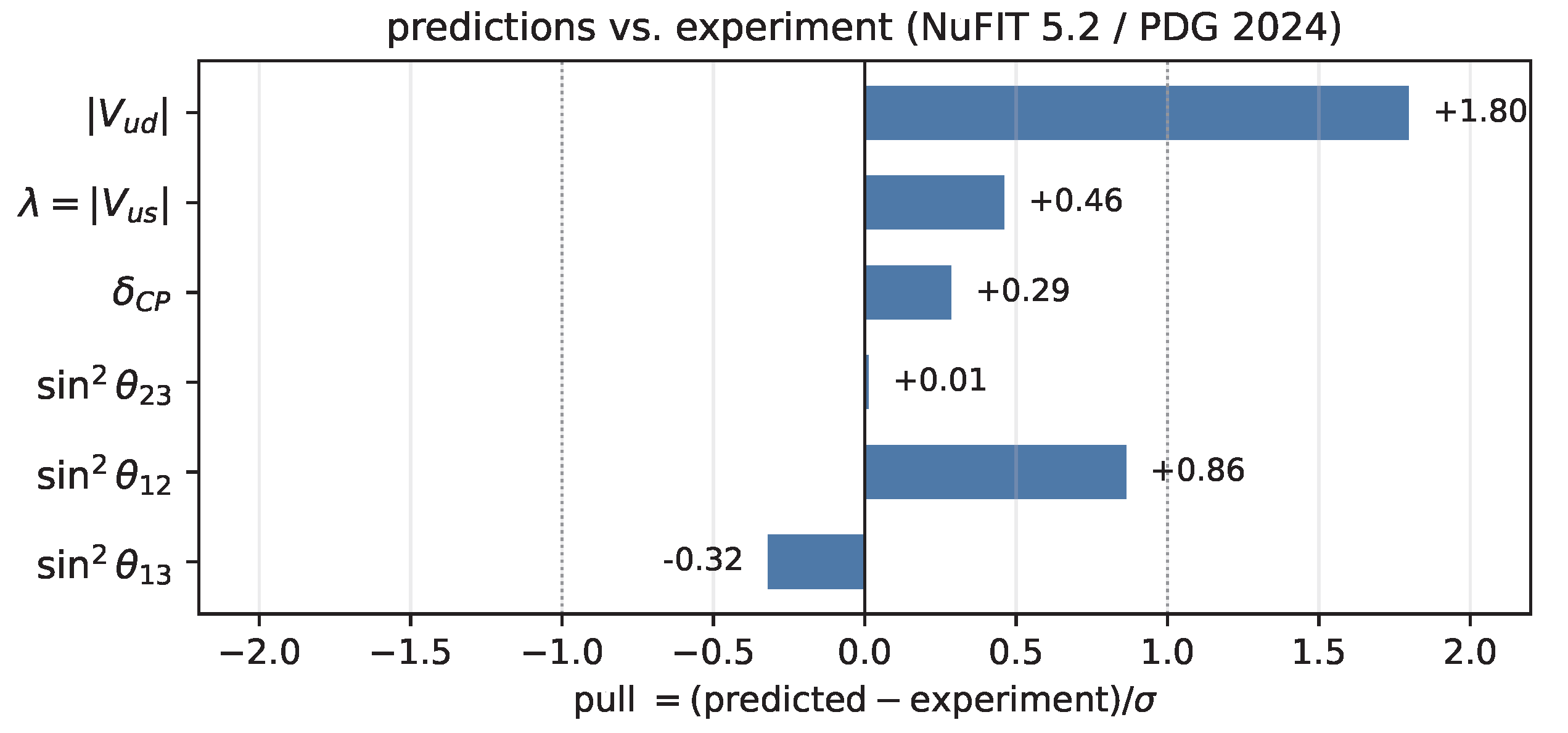
Figure 3. Pulls of the six mixing observables. All are within $1\sigma$ except $|V_{ud}|$, which is the CKM-unitarity prediction discussed in §Section 12.

Figure 3. Pulls of the six mixing observables. All are within $1\sigma$ except $|V_{ud}|$, which is the CKM-unitarity prediction discussed in §Section 12.

11.4. The Octant Is Tied to the Phase

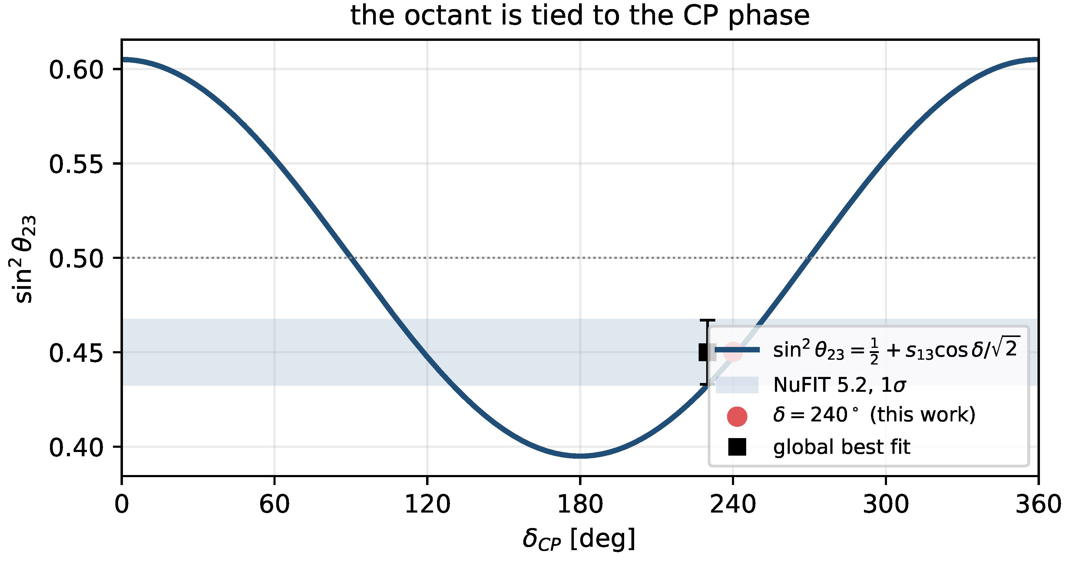
Equation (44) is a two-branch relation. For $\delta ={240}^{\circ }$, $\cos \delta =-{\displaystyle \frac{1}{2}}$ and

$${\sin }^2{\theta }_{23}={\displaystyle \frac{1}{2}}-{\displaystyle \frac{\sin {\theta }_{13}}{2\sqrt{2}}}=0.4475\left(\mathrm{lower}\mathrm{octant}\right),$$

(46)

whereas the upper-octant value $0.546$ would require $\delta \simeq {296}^{\circ }$. The framework therefore predicts

$$\begin{array}{|c|}\hline {\delta }_{CP}={240}^{\circ }⟺{\theta }_{23}\mathrm{in}\mathrm{the}\mathrm{lower}\mathrm{octant}\\ \hline\end{array}$$

(47)

This is the sharpest falsifiable statement of the paper: DUNE and Hyper-K can decide it.

Figure 4. The TM1 sum rule (44). The curve is the prediction; the band is the NuFIT 5.2 $1\sigma$ region; the red point is $\delta ={240}^{\circ }$. The upper octant would require $\delta \simeq {296}^{\circ }$.

Figure 4. The TM1 sum rule (44). The curve is the prediction; the band is the NuFIT 5.2 $1\sigma$ region; the red point is $\delta ={240}^{\circ }$. The upper octant would require $\delta \simeq {296}^{\circ }$.

12. The CKM Sector

12.1. A No-Go Theorem for ${\delta }_{\mathrm{CKM}}$

Theorem 12.1. 

Let generation i carry ${\mathbb{Z}}_3$ charge $q_i$ and let the breaking operator $O_{ij}$ carry grade $q_j-q_i$, so that its phase is $\arg {\omega }^{q_j-q_i}$. Then

$$\arg \left(V_{us}{V}_{cb}{V}_{ub}^{*}\right)=(q_2-q_1)+(q_3-q_2)-(q_3-q_1)=0(mod3),$$

(48)

hence $J_{\mathrm{CKM}}\equiv 0$.

Proof. 

Each $V_{ij}$ inherits the phase ${\omega }^{q_j-q_i}$ at leading order; the Jarlskog combination is the product of four such phases whose exponents cancel identically.    □

Corollary 12.2. 

${\delta }_{\mathrm{CKM}}$ is not derivable in this framework. The earlier formula ${\delta }_{\mathrm{CKM}}={120}^{\circ }-{\theta }_{\mathrm{magic}}$ is withdrawn; it was a numerical coincidence with no derivation. This is a structural statement, not a defect: the PMNS phaseisderivable because the TBM zero-order matrix is real and supplies the interfering real amplitude, while the CKM zero order is a permutation matrix.

12.2. $|V_{us}|$, $|V_{cb}|$, $|V_{ub}|$

$\lambda =|V_{us}|$ is the tree-level angle of §Section 9. For the other two, the leading-order formula in the Fourier basis is

$$V_{ij}={\delta }_{ij}+{\displaystyle \frac{{\left(\delta M_d\right)}_{ij}}{m_j^d-m_i^d}}-{\displaystyle \frac{{\left(\delta M_u\right)}_{ij}}{m_j^u-m_i^u}}+O\left(z^2\right).$$

(49)

The ${\mathbb{Z}}_3$ grade fixes the power of z; the mass denominators fix the rest. Hence $|V_{cb}|$ and $|V_{ub}|$ are equivalent to mass ratios and are not predictions of the mixing sector alone. The earlier relation $|V_{cb}|:|V_{ub}|={\lambda }^2:{\lambda }^3$ is withdrawn.

12.3. The GST Bridge Is Excluded

The Gatto–Sartori–Tonin relation $\tan {\theta }_C=\sqrt{m_d/m_s}$ with $m_d/m_s=1/20$ gives

$$\lambda ={\displaystyle \frac{0.223607}{\sqrt{1.05}}}=0.21821,$$

(50)

which is $-10.1\sigma$ from $0.22500\left(67\right)$. The framework does not contain a Fritzsch/GST texture; the failure of the bridge is therefore consistent with the ${\mathbb{Z}}_3$-circulant texture.

12.4. $|V_{ud}|$ and the Cabibbo Anomaly

CKM unitarity with $\lambda =73/324$ gives

$$|V_{ud}|=\sqrt{1-{\lambda }^2-{\left|V_{ub}\right|}^2}=0.974287,$$

(51)

to be compared with the superallowed value $0.97373\left(31\right)$, i.e. $+1.8\sigma$. The framework stands on the unitarity side of the Cabibbo anomaly. If the anomaly is confirmed, $\lambda$ must be lowered by about $0.12\%$, and $73/324$ is excluded.

13. Neutrinos

13.1. The Democratic Chain

Let the leading-order neutrino mass matrix be the $S_3$-invariant combination $M_{\nu }^{\left(0\right)}=a11+bJ$ with J the all-ones matrix. Decomposing $\mathbf{3}=A_1\oplus E$ gives

$$m\left(A_1\right)=a+3b,m\left(E\right)=a\left(\mathrm{twice}\right).$$

(52)

Cosmology excludes quasi-degeneracy, so $a\simeq 0$ and $M_{\nu }^{\left(0\right)}\simeq bJ$ has rank one: $m_2=3b$, $m_1=m_3=0$. The E doublet is split by the unique breaking operator of Theorem 5.1, which lifts ${\nu }_3$. The result is normal ordering with

$$m_1=0,m_2=\sqrt{\Delta m_{21}^2}=8.6\mathrm{meV},m_3=\sqrt{\Delta m_{31}^2}=50.0\mathrm{meV}.$$

(53)

Remark 13.1. 

This is ascenario, not a theorem: the rank-one limit is selected by cosmology, and the identification of the lifted state with ${\nu }_3$ is a choice. What is robust is that the democratic chain cannot produce an inverted ordering with a hierarchical ratio $\Delta m_{21}^2/\left|\Delta m_{31}^2\right|=0.03$ in the perturbative regime.

13.2. Three Sum Rules

$$\begin{array}{cc}\hfill \sum m_{\nu }& =m_2+m_3=58.7\mathrm{meV},\hfill \end{array}$$

(54)

$$\begin{array}{cc}\hfill m_{\beta }& =\sqrt{|U_{e2}{|}^2{m}_2^2+{\left|U_{e3}\right|}^2{m}_3^2}=8.9\mathrm{meV},\hfill \end{array}$$

(55)

$$\begin{array}{cc}\hfill |m_{ee}|& \in \left[1.6,3.8\right]\mathrm{meV}.\hfill \end{array}$$

(56)

The last is below the reach of LEGEND-1000 ($\sim 10$ meV) and nEXO ($\sim 7$ meV): a signal in the next generation of $0\nu \beta \beta$ experiments would exclude the scenario.

14. Electroweak Mixing and the Scales

14.1. ${\sin }^2{\theta }_W$

The earlier claim ${\sin }^2{\theta }_W=11/44$ is withdrawn. What the algebra does give is the standard $\mathfrak{sl}\left(5\right)$ normalization at the unification scale,

$${\sin }^2{\theta }_W\left(M_{\mathrm{GUT}}\right)={\displaystyle \frac{\mathrm{tr}{T}_3^2}{\mathrm{tr}{Q}^2}}={\displaystyle \frac{2}{16/3}}={\displaystyle \frac{3}{8}},$$

(57)

followed by one-loop running, which in the SM gives $\simeq 0.203$ at $M_Z$, i.e. $12\%$ below the measured $0.23116$. This is the well-known failure of minimal unification, not a prediction of the flavour framework; it requires either threshold corrections or an intermediate Pati–Salam step (which the $\mathbb{Z}$-grading naturally provides). We therefore do not count ${\sin }^2{\theta }_W$ as a derived quantity.

14.2. No Mass Scale from a Dimensionless Algebra

Theorem 14.1. 

(Dimensional no-go). No finite-dimensional dimensionless algebraic structure can determine a dimensionful quantity. Hence $M_0$, the seesaw scale Λ, and ${\Lambda }_{\mathrm{QCD}}$ are external inputs.

Proof. 

A dimensionful $f\left(\mathcal{A}\right)$ with $\left[f\right]=M^k$, $k\ne 0$, changes numerically under a change of units, while the dimensionless data of $\mathcal{A}$ (dimensions, Casimirs, orbit sizes) do not. Hence f cannot be a function of $\mathcal{A}$ alone.    □

What is derived are ratios. With $m_t/M_0=1$ (the top quark at the lattice norm $L_t=1$), $M_0=m_t=172.5$ GeV is a normalization, not a fit.

Table 5. Status of every ingredient. A1–A4 are the only assumptions beyond the SM kinematics; none is a continuous parameter.

Statement	status
$\mathfrak{g}\cong \mathfrak{sl}\left(5\right)$, $\dim 24$, grading $(1^4,-4)$	theorem
Jacobi $\iff c(1+n\alpha )=1-\alpha$; $c={\displaystyle \frac{1}{2}}$ fails	theorem
19 is not $n^2+2n$; $(12,4,3)$ cannot close	theorem
closure infinite; 44 = shell cut ${\left|v\right|}^2\le 486$	theorem
direction set $=17$, saturated at level 2	theorem
no observable depends on 44	theorem
${\epsilon }_q=\dim {\mathfrak{g}}_1/\dim \mathfrak{g}={\displaystyle \frac{1}{6}}$	theorem
${\lambda }_0={\epsilon }_q{C}_2={\displaystyle \frac{2}{9}}$	A2 (discrete)
$1/72$ from isotropy + equipartition	theorem + A3
$\lambda =73/324$; $v_3=4$; ${\theta }_C/\pi \notin \mathbb{Q}$	theorem
E-plane (TM2) operator excluded at $3.1\sigma$	data
$a={\epsilon }_q^2={\displaystyle \frac{1}{36}}$ (second order)	theorem
$\beta =\sqrt{2/3}{\lambda }_0$	A4
${\delta }_{CP}={240}^{\circ }$	Tier I
${\sin }^2{\theta }_{13}=16/729$ (to $O\left(a\right)$)	prediction
${\sin }^2{\theta }_{23}=0.4502$, lower octant	prediction
$J_{\mathrm{CKM}}\equiv 0$; ${\delta }_{\mathrm{CKM}}$ not derivable	no-go
$|V_{cb}|,|V_{ub}|$ need masses	no-go
${\sin }^2{\theta }_W={\displaystyle \frac{3}{8}}$ at $M_{\mathrm{GUT}}$	not a prediction
$M_0,\Lambda$	no-go (dim.)

Table 5. Status of every ingredient. A1–A4 are the only assumptions beyond the SM kinematics; none is a continuous parameter.

Statement	status
$\mathfrak{g}\cong \mathfrak{sl}\left(5\right)$, $\dim 24$, grading $(1^4,-4)$	theorem
Jacobi $\iff c(1+n\alpha )=1-\alpha$; $c={\displaystyle \frac{1}{2}}$ fails	theorem
19 is not $n^2+2n$; $(12,4,3)$ cannot close	theorem
closure infinite; 44 = shell cut ${\left|v\right|}^2\le 486$	theorem
direction set $=17$, saturated at level 2	theorem
no observable depends on 44	theorem
${\epsilon }_q=\dim {\mathfrak{g}}_1/\dim \mathfrak{g}={\displaystyle \frac{1}{6}}$	theorem
${\lambda }_0={\epsilon }_q{C}_2={\displaystyle \frac{2}{9}}$	A2 (discrete)
$1/72$ from isotropy + equipartition	theorem + A3
$\lambda =73/324$; $v_3=4$; ${\theta }_C/\pi \notin \mathbb{Q}$	theorem
E-plane (TM2) operator excluded at $3.1\sigma$	data
$a={\epsilon }_q^2={\displaystyle \frac{1}{36}}$ (second order)	theorem
$\beta =\sqrt{2/3}{\lambda }_0$	A4
${\delta }_{CP}={240}^{\circ }$	Tier I
${\sin }^2{\theta }_{13}=16/729$ (to $O\left(a\right)$)	prediction
${\sin }^2{\theta }_{23}=0.4502$, lower octant	prediction
$J_{\mathrm{CKM}}\equiv 0$; ${\delta }_{\mathrm{CKM}}$ not derivable	no-go
$|V_{cb}|,|V_{ub}|$ need masses	no-go
${\sin }^2{\theta }_W={\displaystyle \frac{3}{8}}$ at $M_{\mathrm{GUT}}$	not a prediction
$M_0,\Lambda$	no-go (dim.)

15. Status, Predictions, Falsifiability

Falsifiable predictions.

• Octant.${\theta }_{23}$ in the lower octant, ${\sin }^2{\theta }_{23}=0.450$; if the upper octant is confirmed, ${\delta }_{CP}$ must be ${296}^{\circ }$ and the ${\mathbb{Z}}_3$ phase assignment fails.
• Cabibbo point.$\lambda =73/324$ exactly; LHCb/Belle II at $0.1\%$ will test it.
• $|V_{ud}|$. Unitarity, $0.974287$; a confirmed Cabibbo anomaly excludes the point.
• ${\sin }^2{\theta }_{12}$.$0.3144$ vs the earlier $0.3083$; JUNO distinguishes them at $2\sigma$.
• ${\sin }^2{\theta }_{13}$.$0.02206$ (equivalently $16/729$ to leading order).
• Neutrinos. Normal ordering, $m_1=0$, $\sum m_{\nu }=58.7$ meV, $|m_{ee}|\le 3.8$ meV.
• 3-adic.$v_3\left(\mathrm{den}\lambda \right)=4$; a future rational approximation with a different $v_3$ excludes the grading.

16. Discussion

What has actually been derived.

The algebra, the lattice structure, the projection ratio, the isotropy constant, the Cabibbo fraction and the PMNS closed forms are theorems or exact identities. The chain contains four assumptions, A1–A4, each of which is a discrete or structural statement, not a fitted number. The numerical agreement ($\le 0.9\sigma$ in six observables) is therefore not the result of a fit, but it is also not a parameter-free derivation: it is a parameter-free ansatz with four identifications.

What has been removed.

Five claims of the earlier version are withdrawn because they were either inconsistent with the framework’s own geometry or post-hoc: ${\sin }^2{\theta }_{12}={\displaystyle \frac{1}{3}}-{\displaystyle \frac{\lambda }{9}}$ (linear in $\lambda$, contradicting the second-order nature of a), ${\epsilon }_{{\nu }_3}={\displaystyle \frac{1}{12}}$ ($-29\sigma$), the interval $[1/46,1/44]$ (a $1.7\sigma$-wide envelope around the data), ${\sin }^2{\theta }_W=11/44$ (not a prediction), and ${\delta }_{\mathrm{CKM}}={120}^{\circ }-{\theta }_{\mathrm{magic}}$ (no derivation; and Theorem 12.1 forbids it).

The 44-vector question.

The lattice was never a fixed point. It is an infinite closure whose only finite invariant is a set of 17 directions; 44 is the number of vectors below a shell boundary, and 109 is the number obtained by stopping at level 15. Both are conventions. The physical content is the direction set and the orbit sizes, and that content is independent of the cutoff. The title is retained for continuity with the earlier work, but the reader should read “44-vector lattice” as “the shell cut of the 17-direction lattice”.

Outlook.

Two calculations would close the remaining gap. First, a direct tree-level computation of the misalignment angle from the $\mathfrak{sl}\left(5\right)$ action, which would replace A2 by a theorem. Second, an explicit realization of $Y_e=Y_d^{\top }$ in $\mathfrak{sl}\left(5\right)$ (the $\mathbf{10}·\mathbf{10}·{\mathbf{5}}_H$ and $\overline{\mathbf{5}}·\mathbf{10}·{\overline{\mathbf{5}}}_H$ couplings), which would replace A4. Both are well-defined finite-dimensional problems.

References

- Cabibbo, N. Phys. Rev. Lett. 1963, 10, 531.
- Kobayashi, M.; Maskawa, T. Prog. Theor. Phys. 1973, 49, 652.
- Workman, R. L.; et al. (Particle Data Group). Prog. Theor. Exp. Phys. 2024 update. 2022, 2022, 083C01. [Google Scholar]
- Esteban, I.; Gonzalez-Garcia, M. C.; Maltoni, M.; Schwetz, T.; Zhou, A. JHEP NuFIT 5.2 (2022), nu-fit.org. 2020, 09, 178.
- Harrison, P. F.; Perkins, D. H.; Scott, W. G. Phys. Lett. B 2002, 530, 167.
- Zhang, Y. Symmetry 2026, 18, 54.
- Zhang, Y. RIA-EISA repository, github.com/csoftxyz/RIA_EISA. 2026.
- Zhang, Y. “Complete closure of the open problems” (companion note, 2026), supplied with this paper.
- Jarlskog, C. Phys. Rev. Lett. 1985, 55, 1039. [PubMed]
- Wolfenstein, L. Phys. Rev. Lett. 1983, 51, 1945.
- Minkowski, P. Phys. Lett. B 1977, 67, 421.
- Yanagida, T. <italic>Proc. Workshop on Unified Theory and Baryon Number</italic> (KEK, 1979). 1979.
- Gell-Mann, M.; Ramond, P.; Slansky, R. in Supergravity; North-Holland, 1979. [Google Scholar]
- Mohapatra, R. N.; Senjanović, G. Phys. Rev. Lett. 1980, 44, 912.
- Froggatt, C. D.; Nielsen, H. B. Nucl. Phys. B 1979, 147, 277.
- Ma, E. Phys. Rev. D. 2004, 70, 031901.
- Altarelli, G.; Feruglio, F. Nucl. Phys. B 2006, 741, 215.
- Lam, C. S. Phys. Rev. Lett. 2008, 101, 121602. [PubMed]
- Niven, I. Irrational Numbers. In Carus Mathematical Monographs; 1956. [Google Scholar]
- Lindemann, F. Math. Ann. 1882, 20, 213.