Submitted:
17 June 2026
Posted:
18 June 2026
You are already at the latest version
Abstract
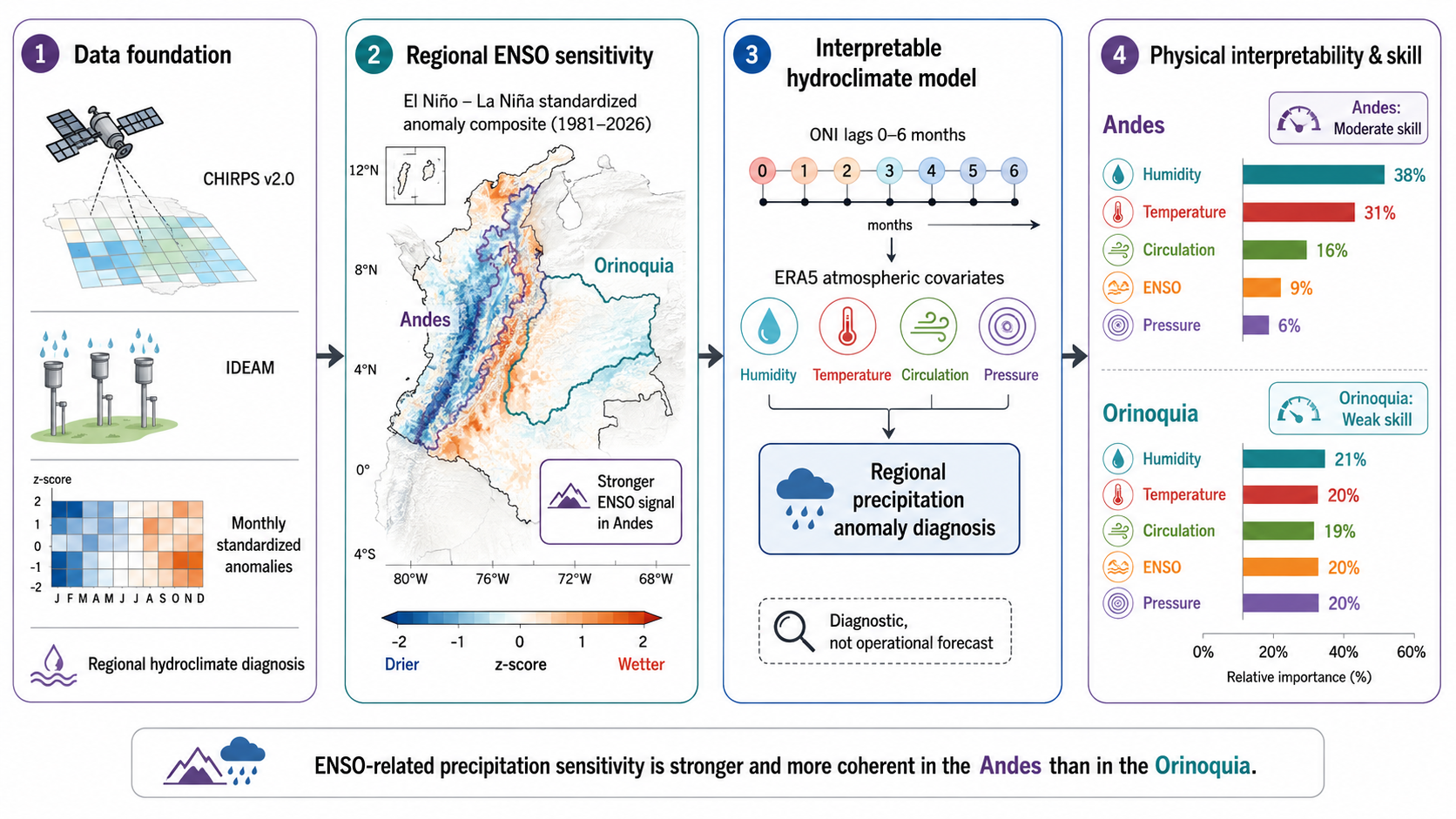
El Niño–Southern Oscillation (ENSO) modulates tropical South American rainfall, but its Colombian expression is filtered by terrain, rainfall regime, moisture pathways, and atmospheric state. We quantify ENSO-related sensitivity of standardized precipitation anomalies in the Colombian Andes and Orinoquia using Climate Hazards Group InfraRed Precipitation with Station data (CHIRPS v2.0; 1981–February 2026), station records from Colombia’s Institute of Hydrology, Meteorology and Environmental Studies (IDEAM), ERA5 predictors, and 1981–2010 climatologies. CHIRPS reproduced station-derived standardized anomalies (r=0.94 in the Andes; r=0.91 in Orinoquia), supporting regional anomaly analysis while retaining cautious comparison framing. Lagged associations with the Oceanic Niño Index (ONI) were evaluated for lags 0–6 months using effective degrees of freedom, block-bootstrap confidence intervals, and maximum-lag tests. ENSO sensitivity was stronger and more coherent in the Andes: annual lag-1 ONI–precipitation correlation was −0.374, with marked December–February and June–August responses. Orinoquia showed weaker annual sensitivity and a season-specific September–November response. Diagnostic models showed modest, temporally cautious skill gains from physically interpretable climate-index and reanalysis predictors in the Andes. ENSO-related Colombian precipitation sensitivity is heterogeneous, lagged, and physically mediated rather than spatially uniform.
Keywords:
ENSO
; CHIRPS
; Andes
; Orinoquia
; precipitation anomalies
; interpretable statistical modeling
; hydroclimate sensitivity
1. Introduction
El Niño–Southern Oscillation (ENSO) is a major source of interannual rainfall variability across tropical South America, including Colombia, where it affects precipitation, streamflow, soil moisture, drought risk, flood risk, ecosystems, hydropower, and agricultural planning [1,2,3,4,5,6]. Its hydroclimatic expression, however, is not spatially uniform and depends strongly on regional circulation, topography, moisture transport pathways, and convective organization across tropical South America [6,7,8]. These studies further emphasize that ENSO teleconnections may vary substantially across regions depending on the interaction between large-scale SST forcing and local hydroclimatic processes.
Colombian precipitation emerges from the interaction of remote Pacific forcing with topography, moisture availability, atmospheric stability, low-level circulation, convective organization, and seasonal migration of tropical convergence zones [9,10,11,12,13]. Recent studies further indicate that deep convection over northwestern South America is strongly modulated by terrain complexity, regional moisture transport, and atmospheric thermodynamic structure, producing highly heterogeneous rainfall responses across the Andes, Pacific coast, Caribbean lowlands, and Amazon–Orinoquia transition zones [13,14]. ENSO is therefore treated here as a large-scale forcing that modulates convection-favorable environments rather than as a direct or exclusive cause of monthly rainfall anomalies.
The Colombian Andes and Orinoquia provide a clear regional contrast for examining this problem. The Andes combine steep terrain, inter-Andean valleys, elevation-dependent climate gradients, and strong orographic modulation of moisture transported from the tropical Pacific, Amazon Basin, and Caribbean Sea. In contrast, the Orinoquia is a lower-elevation eastern lowland domain characterized by a more unimodal rainfall regime, extensive savanna ecosystems, continental moisture recycling, Amazonian and Atlantic moisture pathways, and stronger dependence on regional circulation and convective organization [12,15,16,17,18]. Recent regional studies additionally suggest that precipitation variability across eastern Colombia is strongly influenced by low-level circulation, Amazonian moisture transport, and seasonal hydroclimatic variability associated with tropical lowland dynamics [15,17,18]. Lowland precipitation variability may additionally be affected by intraseasonal tropical variability, including Madden–Julian Oscillation (MJO) modulation of convection and moisture transport across tropical South America [19,20,21,22,23]. These regional contrasts motivate an analysis that moves beyond national-scale ENSO generalizations and instead investigates whether the same large-scale sea surface temperature (SST) forcing is expressed through distinct monthly precipitation-anomaly pathways.
Previous studies have documented ENSO–precipitation relationships in Colombia and the tropical Andes [1,4,5,10,24]; however, four issues remain central to a publication-grade regional diagnosis. First, broad Colombia-wide or Andean-scale statements may obscure contrasts between complex mountainous terrain and eastern lowland hydroclimates. Second, satellite–gauge products such as Climate Hazards Group InfraRed Precipitation with Station data (CHIRPS) should be evaluated against national observations while acknowledging that station records may not be fully independent of the calibration sources used in gridded precipitation products [25,26,27,28,29,30,31,32]. Third, lagged ENSO correlations require explicit treatment of autocorrelation and objective lag-selection criteria. Finally, predictive models may help identify whether atmospheric-state variables provide physically interpretable information beyond the Oceanic Niño Index (ONI); however, such models should be framed as diagnostic tools rather than as causal or operational forecasting systems [33]. In particular, monthly atmospheric diagnostics derived from reanalysis products cannot fully resolve mesoscale convective systems, convection-permitting dynamics, or the strong diurnal-cycle organization of precipitation known to characterize the tropical Andes and adjacent lowlands [13,14].
This study addresses these issues through a reproducible, hydroclimate-focused workflow. The central research question is: how does the sensitivity of monthly standardized precipitation anomalies to ENSO differ between the Colombian Andes and the Orinoquia, and to what extent do physically interpretable atmospheric and climate-index predictors help explain this regional contrast? We test three linked hypotheses: (i) ENSO-related sensitivity is stronger and more spatially coherent in the Andes than in the Orinoquia; (ii) the dominant ONI lag relationships remain robust after accounting for serial dependence and lag-selection effects; and (iii) European Centre for Medium-Range Weather Forecasts fifth-generation reanalysis (ERA5) variables and climate-index predictors provide measurable diagnostic information without supporting causal or operational forecasting claims. Together, these analyses evaluate whether ENSO-related precipitation sensitivity in Colombia is regionally heterogeneous, temporally lagged, and physically interpretable rather than spatially uniform.
2. Materials and Methods
2.1. Study Area and Regional Domains
The analysis focuses on two hydroclimatically contrasting regions within continental Colombia: the Colombian Andes and the Orinoquia (Figure 1). The Andes domain is an administrative-hydroclimatic mask centered on the three cordilleras—the Western, Central, and Eastern Cordilleras—and the intervening Magdalena and Cauca valleys, extending from approximately N to N and from W to W, and covering roughly 280,000 km2. Elevations range from 200 m in the valley floors to more than 5,000 m at the highest peaks. This domain is characterized by complex topography, steep elevation gradients, and a bimodal precipitation regime driven by the meridional migration of the Intertropical Convergence Zone (ITCZ), with two wet seasons (March–May and September–November) and two relatively drier periods (December–February and June–August). The Andes domain exhibits documented sensitivity to ENSO variability, with El Niño typically associated with negative precipitation anomalies and La Niña with positive anomalies [4,9,11].
The Orinoquia domain covers the eastern lowlands of Colombia, extending from the eastern flank of the Eastern Cordillera (∼ W) to the Venezuelan border (∼ W), and from the Arauca River in the north (∼ N) to the Guaviare River in the south (∼ N), encompassing approximately 255,000 km2. The region is characterized by a unimodal precipitation regime, with a single wet season from May to September and a pronounced dry season from December to March, extensive savanna ecosystems (Llanos Orientales), sparse rain-gauge coverage, and strong seasonal rainfall variability [15,18]. Elevations range from approximately 50 m to 500 m above sea level, and the landscape is dominated by alluvial plains, dissected terraces, and isolated remnants of the Guiana Shield.
This physiographic and climatic contrast is central to the objective of this study: to quantify where and why standardized monthly precipitation anomalies respond differently to ENSO forcing across these two domains. The Andes are strongly influenced by orographic lifting and regionally organized moisture transport from the tropical Pacific, Amazon Basin, and Caribbean Sea, whereas rainfall in the Orinoquia is more closely associated with lowland seasonality, continental moisture recycling, Atlantic–Amazonian transport pathways, and regional atmospheric circulation [12,16,17]. In the Andes, orographic uplift of moisture-laden air masses generates precipitation that is sensitive to changes in moisture availability, atmospheric stability, and low-level wind direction, all of which may be modulated by ENSO-related Pacific SST anomalies. This interpretation is consistent with previous hydroclimatic studies showing that ENSO modulates regional moisture transport, atmospheric stability, and precipitation efficiency over the tropical Andes and northwestern South America [4,12,13]. In contrast, precipitation in the Orinoquia is governed more strongly by large-scale convergence, the seasonal migration of the ITCZ, low-level wind fields, and local-to-mesoscale convective organization over the eastern plains, making the ENSO signal less direct and more intertwined with regional and continental-scale processes. Intraseasonal tropical variability, including Madden–Julian Oscillation (MJO) modulation of convection and moisture transport, may additionally contribute to rainfall organization across the eastern plains and northern tropical South America [19,20,21,22,23].
Region masks were constructed by dissolving IGAC departmental boundaries: Antioquia, Boyacá, Caldas, Cauca, Cundinamarca, Huila, Nariño, Norte de Santander, Quindío, Risaralda, Santander, Tolima, and Valle del Cauca for the Andes; and Arauca, Casanare, Meta, and Vichada for the Orinoquia. These polygons were used to aggregate CHIRPS precipitation and ERA5 atmospheric variables into monthly regional time series. Because the masks represent administrative approximations of broad hydroclimatic domains rather than strict physiographic boundaries, the regional aggregation is intentionally diagnostic: it evaluates whether these contrasting large-scale settings exhibit different ENSO responses before moving toward finer subregional or topography-aware analyses. Key regional characteristics are summarized in Table 1.
Topography is retained throughout this study as a static physiographic context, not as a temporal predictor. The spatial modulation of ENSO sensitivity by topographic gradients, including elevation-dependent teleconnection strength and orographic enhancement of precipitation anomalies, constitutes a natural extension of the present regional framework and is deferred to future work.
2.2. Precipitation Data and IDEAM Comparison
CHIRPS v2.0 monthly precipitation totals were used as the primary gridded precipitation dataset because the product provides long-term, spatially continuous coverage at approximately resolution from 1981 onward [25]. CHIRPS was used to compute monthly climatologies, standardized anomalies, spatial composites, and regional time series. IDEAM station observations and an IDEAM-associated gridded product were used to assess whether CHIRPS provides sufficient consistency for regional hydroclimatic analysis.
We refer to this step as a CHIRPS–IDEAM comparison or evaluation rather than a strict independent validation. Because IDEAM station data may contribute directly or indirectly to the gauge-adjustment or calibration procedures used in CHIRPS, station–pixel agreement could overestimate fully independent performance. This limitation does not preclude the use of CHIRPS for regional anomaly analysis; however, it requires cautious interpretation and transparent reporting of uncertainty.
2.3. ENSO, ERA5, and Climate-Index Predictors
ONI was the primary ENSO index, defined as the 3-month running mean of sea surface temperature (SST) anomalies in the Niño 3.4 region provided by the National Oceanic and Atmospheric Administration (NOAA). Monthly ONI values were matched to precipitation anomalies and lagged from 0 to 6 months to account for delayed hydroclimatic responses [2,10]. For any climate index , the lagged predictor was defined as:
where represents the lag in months, is the value of climate index k at calendar month t, and is the lagged predictor used in the models. Positive lag values indicate precipitation anomalies evaluated after the corresponding climate-index state.
A multi-index climate set, including the Pacific Decadal Oscillation (PDO), Atlantic Multidecadal Oscillation (AMO), Multivariate ENSO Index (MEI), Southern Oscillation Index (SOI), and the Niño 1+2, Niño 3, and Niño 4 SST regions, was incorporated where available and quality-checked. This multi-index framework provides complementary representation of Pacific and Atlantic climate variability while acknowledging ENSO diversity and spatial heterogeneity [6,7,8].
Monthly ERA5 reanalysis fields at (∼28 km) were used to provide regional atmospheric context [34]. The following variables were averaged spatially over each domain: 2-m temperature, specific humidity, dewpoint temperature, 10-m zonal and meridional wind components, and surface pressure. These variables were not used as primary ENSO predictors but as covariates in multi-index modeling to support physical interpretation [12,17]. ERA5 variables do not diagnose individual convective storms; they represent monthly-scale atmospheric states relevant to precipitation anomalies. The ERA5 covariate vector is:
where is the 2-m air temperature (K), is the 2-m dewpoint temperature (K), q is the specific humidity, and are the 10-m zonal and meridional wind components (m s−1), and is the surface pressure (hPa). All variables are spatially averaged over region r at month t. This formulation provides a physical bridge linking ENSO-related climate forcing to regional moisture availability, thermodynamic state, and low-level circulation, but it does not directly compute moisture convergence, convective available potential energy, storm organization, or cloud microphysics.
ENSO phase composites used monthly ONI thresholds of at least C for El Niño conditions, at most − C for La Niña conditions, and intermediate values for Neutral conditions. These categories are used for composite interpretation rather than as formal CPC event declarations. ONI remains the primary ENSO variable for the main inference. Datasets, periods, and roles are summarized in Table 2.
2.4. Monthly Climatology and Standardized Precipitation Anomalies
Monthly CHIRPS precipitation was converted into standardized anomalies using a 1981–2010 climatological baseline. For each grid cell and calendar month, the mean and standard deviation were computed over the baseline period. Standardized anomalies were then calculated as:
where is the monthly precipitation total for pixel p, calendar month m, and year y; and are the baseline mean and standard deviation. Months with fewer than 15 years of valid baseline data were excluded to avoid unstable standardization. Anomalies are expressed in dimensionless z units.
2.5. Regional Aggregation
Pixel-level monthly z-scores were spatially averaged over the Andes and Orinoquia domains separately using the regional masks defined in Section 2.1. The resulting regional series represent the monthly standardized anomaly for each domain. No area-weighting was applied given the high-resolution CHIRPS grid and the well-defined regional boundaries. The regional anomaly used in the temporal analyses is:
where is the standardized anomaly for region r at month t, is the pixel-level standardized anomaly, and is the number of valid CHIRPS pixels inside the regional mask at that time step.
2.6. CHIRPS–IDEAM Comparison
CHIRPS was evaluated against IDEAM-associated gridded and station records. For the gridded comparison, CHIRPS standardized anomalies were converted back to precipitation units using the CHIRPS climatological mean and standard deviation and compared with the IDEAM-associated gridded reference over overlapping months. For the station–pixel comparison, IDEAM monthly station precipitation was paired with the corresponding CHIRPS grid cell and summarized by region. The main text emphasizes correlation, bias, and error magnitude; extended metrics are retained in the supplementary material.
2.7. Robust ENSO Lag-Correlation Inference
ENSO sensitivity was quantified using correlations between monthly standardized precipitation anomalies and ONI lags from 0 to 6 months. Pearson and Spearman correlations were computed for annual and seasonal subsets (DJF, MAM, JJA, SON). For each region r, season s, and lag ℓ:
where is the Pearson correlation coefficient for region r during season s at lag ℓ; is the regional standardized precipitation anomaly for months belonging to season s; and is the Oceanic Niño Index lagged by ℓ months.
Because monthly time series and ONI are autocorrelated, Pearson significance was adjusted using effective sample size [35,36]. Twelve-month block-bootstrap confidence intervals characterized uncertainty in correlation estimates. To account for lag selection, the analysis used a circular-shift maximum-absolute-lag test with 1000 permutations: within each region and season, the statistic of interest was the largest absolute correlation among ONI lags 0–6. False-discovery-rate summaries were computed for explicit region–season–lag hypothesis families [37].
2.8. Seasonal Hydroclimatic Composites
Seasonal spatial context was evaluated in two steps. First, DJF, MAM, JJA, and SON CHIRPS climatological precipitation fields were computed from the 1981–2010 monthly baseline to define the background hydroclimatic regimes. Second, seasonal standardized-anomaly composites were computed for El Niño, Neutral, and La Niña months. Neutral conditions were retained as a hydroclimatic baseline, not merely as a residual category, because they help distinguish ENSO-related organization from the background seasonal anomaly structure.
2.9. Interpretable Predictive Modeling
Predictive models were used as diagnostic tests of whether physically interpretable predictors add information beyond ONI alone. Three predictor sets were compared: ONI-only, ONI plus ERA5, and climate indices plus ERA5. A zero-anomaly baseline anchored skill estimates. Linear regression, Ridge, and ElasticNet were treated as the primary interpretable model families [38]; generalized additive and tree-based models were retained as supporting sensitivity analyses rather than as the main scientific claim [39,40,41].
The general diagnostic model can be written as:
where is the predicted standardized anomaly for region r at month t; is the vector of ONI and optional multi-index predictors at lags 0 through 6 months; is the ERA5 atmospheric-state vector (Equation 2); and denotes the fitted regression model with parameters .
Hyperparameters were selected only within the training period using time-series cross-validation. Performance was assessed using a fixed temporal split, with 1981–2010 used for training and 2011–February 2026 used for out-of-sample testing, and with nested expanding-window summaries used to evaluate temporal stability. Model skill was summarized using the following metrics, all computed on held-out walk-forward test samples:
where is the predicted standardized anomaly, is the observed value, is the mean of observed values, and n is the number of test observations.
2.10. Interpretability and Physical Contribution
Predictor contributions were summarized by physically meaningful families: ENSO, humidity, temperature, circulation, and pressure. Coefficients and global interpretability summaries were used to compare regional predictor signatures. SHAP (SHapley Additive exPlanations) values [42] were used to decompose predictions across physical families.
For coefficient-based summaries, the family contribution was computed as:
where g is a physical predictor family (ENSO, humidity, temperature, circulation, or pressure), is the standardized regression coefficient of predictor j, and is the total absolute contribution of family g. For SHAP-based summaries, the analogous family contribution was:
where is the SHAP value of predictor j for observation t, and n is the number of test observations. These quantities describe diagnostic contribution magnitudes; they do not represent causal effects. SHAP-style outputs are retained as supporting material rather than as a central modeling result.
3. Results
3.1. CHIRPS Supports Regional Anomaly Analysis After IDEAM Comparison
The observational backbone of this study is the IDEAM rain-gauge network, whose spatial distribution is shown in Figure 2. The Andes domain contains substantially more stations (2,034 valid stations) than the Orinoquia (153 stations), reflecting differences in historical monitoring density and topographic accessibility. Despite this disparity, both regions retain sufficient observational coverage for the comparison strategy described in Section 2.
The station–pixel comparison indicates that CHIRPS reproduces monthly precipitation variability with sufficient fidelity for regional hydroclimatic diagnosis, although the evidence is interpreted as agreement rather than strict independent validation. Figure 3 summarizes station-level Pearson correlations and RMSE distributions for IDEAM–CHIRPS monthly precipitation agreement across the Andes and Orinoquia regions. The Andes region contains 665,839 monthly station–pixel pairs, with a median station–pixel correlation of 0.814 and a median RMSE of 60.4 mm month−1. The Orinoquia, with 56,318 pairs, exhibits a higher median correlation () but larger absolute errors (median RMSE = 81.4 mm month−1), consistent with the higher rainfall totals characteristic of the lowlands. Kling–Gupta Efficiency (KGE) values of 0.648 for the Andes and 0.792 for the Orinoquia provide an additional summary measure of station–pixel agreement [43]. These results remain stable across minimum-record-length thresholds ranging from 36 to 240 months: median correlations remain near 0.81 in the Andes and 0.88 in the Orinoquia, while median RMSE values remain close to 60–61 mm month−1 and 79–81 mm month−1, respectively. Seasonal station–pixel correlations remain positive throughout all seasons in both regions, although wet-season errors are larger in the Orinoquia, reinforcing the need for cautious interpretation where station density is low and rainfall totals are high.
The standardized-anomaly comparison constitutes the more relevant test for the ENSO workflow because it evaluates the response variable used throughout the study (Figure 4). Monthly regional station-derived anomalies are strongly consistent with nearest-pixel CHIRPS anomalies: the Andes exhibits and the Orinoquia , both with . RMSE values in standardized-anomaly (z-score) units are 0.304 for the Andes and 0.338 for the Orinoquia, while mean bias remains near zero in both regions.
These results support the use of CHIRPS for regional anomaly analysis, although the comparison is still interpreted cautiously because full station independence from CHIRPS/GPCC calibration pathways cannot be assumed. Figure 3 summarizes regional station–pixel correlation and RMSE distributions, complementing the spatial bias patterns shown in Figure 2.
3.2. ENSO-Related Anomaly Organization Is Stronger in the Andes
Seasonal climatology provides the hydroclimatic context needed to interpret how ENSO-related precipitation anomalies emerge across the Andes and Orinoquia (Figure 5). Figure 5 is arranged as a 4 × 4 matrix: rows correspond to the four standard meteorological seasons (DJF, MAM, JJA, SON), and columns separate the climatological baseline from the ENSO-phase anomaly composites.
The first column of Figure 5 presents the seasonal climatology for each season. The two regions exhibit markedly different rainfall regimes. In the Andes, precipitation is spatially heterogeneous and strongly influenced by elevation gradients, orographic lifting, and the interaction of moisture transport from the tropical Pacific, Amazon Basin, and Caribbean Sea with complex terrain. In contrast, the Orinoquia is dominated by a spatially more uniform lowland regime characterized by broad savanna plains, a pronounced wet–dry seasonal cycle, and stronger dependence on continental-scale moisture transport and large-scale atmospheric convergence.
These contrasts are evident across the seasonal cycle. During DJF, the Andes maintain moderate rainfall (100–250 mm month−1 on the eastern slopes), whereas the Orinoquia experiences its driest conditions of the annual cycle (<50 mm month−1), associated with the southernmost ITCZ position. MAM represents the transition toward wetter conditions in both regions, particularly along the eastern Andean slopes and the Orinoquia piedmont where precipitation increases substantially. During JJA, the Orinoquia reaches its seasonal rainfall maximum (>300 mm month−1) as the unimodal wet season intensifies across the eastern plains, while parts of the Andes experience relative drying associated with the veranillo (mid-summer dry spell). In SON, precipitation increases again across much of the Andes, while rainfall in the Orinoquia gradually weakens, reinforcing the contrasting bimodal versus unimodal seasonal structures of the two domains.
The second column of Figure 5 displays standardized precipitation anomaly composites (z-scores) for months classified as El Niño under the ONI ±C threshold. During El Niño, negative anomalies predominate across the Andes in all four seasons, with the strongest and most spatially coherent signals in DJF and JJA, where portions of the central and eastern cordilleras fall below . The western slopes of the Western Cordillera and the Pacific lowlands exhibit weaker anomalies, suggesting an orographic modulation of the ENSO teleconnection. In the Orinoquia, negative anomalies are present in DJF and SON but are weaker in magnitude and less spatially organized; during MAM and JJA the El Niño anomaly field is closer to the background state.
The third column of Figure 5 shows composites for months in which ONI remains between and C. Anomaly magnitudes are near zero across all seasons and grid cells, confirming that the compositing procedure is not affected by residual phase-classification artifacts or persistent biases in the reference climatology. This panel thus serves as an observational control, demonstrating that the El Niño and La Niña signals described here emerge from the phase classification rather than from intrinsic spatial biases in the CHIRPS anomaly field.
The fourth column of Figure 5 displays composites for La Niña months. The pattern is broadly symmetric to that of El Niño but of opposite sign: widespread positive anomalies cover much of the Andes, with the strongest signals again occurring in DJF and JJA where local values exceed . The same spatial gradients observed in the El Niño panels—stronger anomalies over the eastern and central cordilleras and weaker anomalies over the Pacific slope—appear in reverse, indicating a phase-symmetric, approximately linear Andean ENSO response. In the Orinoquia, positive anomalies are discernible in DJF and SON but are muted and spatially incoherent in MAM and JJA, consistent with the weaker overall ENSO sensitivity of the lowlands.
Spatial averaging of the composites within each region polygon confirms the visual contrasts. The Andes El Niño minus La Niña difference reaches in JJA and in DJF, with moderate values in MAM () and SON (). In Orinoquia, the equivalent differences are substantially smaller: DJF (), MAM (), JJA (), and SON (). The seasonal ranking of the Andean differences follows the same order as the robust ONI-lag correlations (Table 3), confirming that the composite-based sensitivity estimates are consistent with the continuous correlation analysis. Overall, the results indicate that ENSO-related precipitation sensitivity in Colombia is strongly region-dependent, with a more coherent and persistent signal in the Andes than in the Orinoquia. The stronger spatial coherence observed across the Andes is physically consistent with previous studies linking ENSO variability with changes in regional moisture transport, atmospheric stability, and organized convection over complex tropical terrain [4,12,13,17]. This weaker and less spatially organized response over the Orinoquia suggests that lowland precipitation variability is more strongly mediated by continental moisture recycling, seasonal low-level circulation, and regional convective organization than by ONI phase alone [15,17,18].
3.3. Regional Standardized Anomalies Define the Hydroclimatic Response
The regional standardized anomaly series define a common response scale for the two domains (Figure 6). Large ENSO episodes align more consistently with sustained Andean anomaly excursions than with Orinoquia anomalies, where high-frequency variability and season-specific behavior are more apparent. The 1981–2010 period defines the climatological baseline and model-training interval, while 2011–February 2026 is reserved for temporal testing.
3.4. Robust ONI Lag Sensitivity Is Stronger in Andes
The mean monthly CHIRPS precipitation cycle (Figure 7a) confirms the contrasting seasonal regimes: the Andes exhibit a bimodal regime with two wet seasons (March–May and September–November) separated by drier DJF and JJA periods, whereas the Orinoquia shows a unimodal regime with a single wet season from May to September and a pronounced dry season from December to March. This seasonal structure has direct consequences for how ENSO sensitivity is expressed across the annual cycle: the standard seasonal windows (DJF, MAM, JJA, SON) capture the transitions between wet and dry periods differently in each domain, which must be considered when interpreting lagged correlations.
Robust lag inference confirms that the Andean ENSO signal is negative, lagged, and seasonally organized (Table 3, Figure 7b,c). Annually, the Andes have a best lag of 1 month (; 95% block-bootstrap CI: to ; maximum-lag ). DJF and JJA are the clearest seasonal expressions, with DJF peaking at lag 2 () and JJA at lag 1 (). SON is also robust at lag 4 (), whereas MAM is weaker and does not pass the same maximum-lag threshold. Optimal lags vary seasonally, suggesting that the atmospheric bridge linking tropical Pacific SST anomalies to Andean precipitation operates with region- and season-specific timing. Such lagged responses are physically plausible because ENSO-related SST anomalies may first alter large-scale circulation, thermodynamic structure, and moisture transport before influencing regional precipitation organization over the Andes [4,12,13].
Orinoquia correlations are consistently weaker. The annual best-lag association is small ( at lag 1), and the clearest seasonal signal occurs in SON (lag 4, ). DJF is weak, while MAM and JJA do not show robust ONI sensitivity under the maximum-lag test. This pattern confirms the fragmented Andes–Orinoquia contrast and indicates that ONI alone provides limited predictive signal for Orinoquia precipitation anomalies. This weaker relationship supports the interpretation that lowland precipitation variability in the Orinoquia is mediated by a broader combination of continental moisture recycling, regional circulation variability, and convective organization processes not fully represented by ONI alone [15,17,18]. The regional contrast persists after accounting for autocorrelation and the search across lags.
In Table 3, the effective sample size is expressed as equivalent independent monthly paired observations after autocorrelation adjustment; it is not a count of years, pixels, or stations. Values can approach the number of available months when the precipitation anomaly series has weak or negative lag-1 autocorrelation.
3.5. Temporal Diagnostic Gain Depends on ENSO Sensitivity and Regional Mediation
Relating seasonal ONI sensitivity to changes in walk-forward model skill helps clarify how the diagnostic framework supports the hydroclimatic interpretation of ENSO-related precipitation variability (Figure 8). Figure 8 summarizes the relationship between robust ONI–precipitation sensitivity and the additional explanatory value obtained when moving from an ONI-only configuration to the expanded predictor framework that incorporates additional climate indices and ERA5 atmospheric variables. The horizontal axis represents the strongest absolute ONI–precipitation correlation identified in the robust lag analysis across lags of 0–6 months, while the vertical axis shows the corresponding change in walk-forward (). Point size scales with the final expanded-model , such that larger symbols indicate seasons with greater overall diagnostic skill.
In the Andes, JJA combines strong ONI sensitivity with the largest positive diagnostic gain from the expanded predictor framework (), indicating that atmospheric-state variables and additional climate modes provide physically relevant information beyond ONI alone during the season of strongest ENSO organization. In contrast, DJF exhibits similarly strong ONI sensitivity but only marginal improvement after including the expanded predictors. This contrast suggests that additional atmospheric variables do not simply reinforce ENSO information uniformly across seasons; rather, their contribution depends on whether regional atmospheric mediation introduces variability not already captured by the tropical Pacific SST signal. The larger gains observed in JJA therefore support the interpretation that moisture transport, circulation structure, and atmospheric-state variability contribute meaningfully to the seasonal organization of Andean precipitation anomalies.
In the Orinoquia, the relationship between ENSO sensitivity and diagnostic gain is weaker and less consistent. Positive gains during MAM and JJA occur despite relatively weak ONI sensitivity and low absolute model skill, whereas DJF and SON exhibit reduced performance relative to the ONI-only configuration. This behavior reinforces the interpretation that precipitation variability in the Orinoquia is not well summarized by a single Pacific SST index and that additional atmospheric and climate predictors provide only partial and season-dependent explanatory power. The comparatively small and unstable gains across seasons are consistent with the weaker spatial coherence of the ENSO composites and with the stronger influence of regional lowland dynamics, continental moisture recycling, and large-scale convergence processes discussed previously.
Overall, the synthesis demonstrates that stronger ENSO sensitivity does not necessarily translate into larger predictive improvement when physically informed atmospheric predictors are introduced. Instead, diagnostic gain emerges selectively in specific seasonal and regional contexts. Seasons with strong ONI sensitivity but limited gain suggest that ENSO alone already explains much of the predictable variance, whereas seasons with moderate ONI sensitivity but measurable improvement indicate that atmospheric-state variables and additional climate modes capture complementary hydroclimatic information not represented by ONI alone. Because rolling and block-validation diagnostics remain substantially more conservative than the fixed temporal split (Supplementary Table S8), the resulting model skill is interpreted cautiously as diagnostic evidence for regional hydroclimatic mediation rather than as stable operational forecasting performance. This restrained interpretation is consistent with recent recommendations emphasizing physically interpretable machine-learning applications in weather and climate science rather than purely predictive black-box frameworks [33]. A summary of fixed-split temporal validation metrics is provided in Table 4.
Regularized models are reported for the higher-dimensional predictor sets to avoid over-interpreting unregularized fits; rolling and block-validation diagnostics in the supplementary material qualify temporal stability.
3.6. Physical Predictor Families Support Regional Hydroclimatic Mediation
The physical-family synthesis links the temporal model results to interpretable hydroclimatic pathways (Figure 9). In the Andes, humidity and temperature terms carry the largest aggregate standardized contributions (0.347 and 0.321, respectively), while ENSO, pressure, and circulation terms remain non-negligible. This structure is consistent with a response in which remote Pacific forcing is expressed through regional atmospheric states that condition convection and orographic rainfall. The dominant role of humidity and thermodynamic predictors is also consistent with previous studies emphasizing the importance of atmospheric moisture availability and regional thermodynamic structure for organized convection over the northern tropical Andes [12,13]. Orinoquia shows smaller and more evenly distributed contributions, with temperature (0.132), humidity (0.127), pressure (0.092), circulation (0.072), and ENSO (0.065) all contributing modestly. This diffuse pattern reinforces the inference that monthly lowland precipitation anomalies are less coherently summarized by ONI and more seasonally mediated by lowland moisture and circulation conditions.
Detailed MAE, RMSE, , correlation, residual diagnostics, and SHAP-style summaries are retained in the supplementary material and reproducible outputs. In the main text, model results support one conservative claim: physically meaningful atmospheric and climate-index predictors provide modest-to-moderate diagnostic gains in selected seasons, but they do not constitute an operational forecasting system and their temporal stability remains limited.
3.7. Andes vs Orinoquia
The results demonstrate a clear and consistent regional contrast in ENSO sensitivity. The Colombian Andes exhibit a robust, negative, seasonally stratified, and lag-dependent association with ENSO, particularly in DJF ( at lag 2) and JJA ( at lag 1), where standardized monthly precipitation anomalies show measurable but limited ONI-only skill and larger, still diagnostic, gains when multi-index and ERA5 covariates are included. The dominance of specific humidity and dewpoint as top predictors (Figure 9) supports a physical pathway in which ENSO-driven changes in moisture availability and low-level stability shape the regional environment for convection over orographic terrain.
The Orinoquia shows a fragmented ENSO association that is weak or non-significant in most seasons, with no robust ONI-only skill and only modest, less temporally stable improvements from expanded predictors. The distributed coefficient pattern across physical families mirrors the weak ONI correlations and suggests that monthly precipitation anomalies in this domain are shaped by a broader set of regional-scale controls. The regional contrast identified throughout the analysis therefore supports the interpretation that ENSO teleconnections in Colombia are hydroclimatically conditioned rather than spatially uniform, with stronger and more coherent organization emerging over the complex terrain of the Andes than over the eastern tropical lowlands [6,7,8]. These findings demonstrate that CHIRPS-based standardized anomalies, evaluated against IDEAM station records, can support a physically interpretable regional diagnosis of ENSO–precipitation sensitivity across two hydroclimatically contrasting Colombian domains.
4. Discussion
4.1. Regional ENSO Sensitivity Is Hydroclimatically Conditioned
The principal result of this study is not simply that one region exhibits stronger ENSO correlations than another, but that the same tropical Pacific forcing is expressed through markedly different hydroclimatic environments. Across the Andes, ENSO sensitivity appears consistently in the spatial composites, regional anomaly time series, robust lag relationships, and diagnostic modeling framework, whereas the Orinoquia exhibits weaker, less spatially coherent, and more season-dependent organization. Together, these results support the interpretation that ENSO teleconnections in Colombia are strongly conditioned by rainfall regime, terrain complexity, atmospheric circulation, and regional hydroclimatic mediation rather than by a spatially uniform SST–precipitation relationship [4,6,7,8].
For the Andes, this interpretation is physically consistent with the regional climatology and with previous studies of convection and circulation over northwestern South America. ENSO-related tropical Pacific SST anomalies can alter the thermodynamic and dynamical environment in which Andean precipitation develops, including moisture transport pathways, lower-tropospheric stability, pressure gradients, low-level wind direction, and the efficiency of orographically forced ascent [4,12,17]. Hernández-Deckers [13] documented reductions in deep convective activity and changes in vertical mass flux over northwestern South America during El Niño conditions, while regional analyses have also linked high-elevation precipitation variability to water-vapor availability and atmospheric stability [44]. The stronger and more persistent ENSO organization observed during DJF and JJA is therefore consistent with a hydroclimatic mediation pathway in which tropical Pacific forcing modifies the large-scale atmospheric environment that controls rainfall generation over complex terrain. Although the present analysis operates at monthly regional scales and cannot resolve storm-scale convection or mesoscale organization explicitly, the combined influence of humidity, temperature, circulation, pressure, and climate-index predictors supports a physically interpretable connection between ENSO variability and Andean hydroclimate.
4.2. Orinoquia Response Is Weaker and More Season-Dependent
The weaker ENSO sensitivity observed in the Orinoquia should not be interpreted as climatic insensitivity, but rather as evidence that monthly precipitation variability in the eastern lowlands is controlled by a broader and more distributed set of hydroclimatic processes. The Orinoquia rainfall regime is strongly influenced by continental moisture recycling, Amazonian and Atlantic moisture transport, low-level circulation, large-scale convergence, surface thermodynamic gradients, and mesoscale convective organization across the eastern plains [12,15,17,18]. Intraseasonal tropical variability, including Madden–Julian Oscillation (MJO) modulation of convection and moisture transport, may additionally contribute to precipitation organization across tropical South America and Colombia [19,20,21,22,23].
Within this setting, monthly precipitation anomalies are not expected to respond linearly or uniformly to a single tropical Pacific SST index. This interpretation is consistent with the weak ONI-only skill, the limited seasonal coherence of the ENSO composites, and the more evenly distributed predictor contributions across physical variable families (Figure 9). Positive diagnostic gains during selected seasons indicate that atmospheric-state variables contain complementary hydroclimatic information beyond ONI alone; however, these gains remain comparatively small and unstable relative to the Andes. The results therefore support a regional interpretation in which ENSO acts as one partial forcing embedded within a more complex lowland hydroclimatic system shaped by continental moisture transport, seasonal circulation variability, and mesoscale convective processes [15,17,18].
Regional aggregation may also obscure important foothill–lowland gradients and localized circulation responses within the Orinoquia domain. In particular, precipitation variability along the Andean piedmont may respond differently to ENSO forcing than the eastern savanna lowlands. Future analyses at subregional or pixel scales could therefore help distinguish topographic-transition processes from broader continental lowland dynamics.
4.3. Interpretable Modeling Clarifies Hydroclimatic Mediation Without Implying Causality
The predictive framework developed here is scientifically useful only insofar as it helps interpret the physical organization of regional hydroclimatic variability. In the Andes, moving from ONI-only predictors to the expanded predictor framework increases diagnostic skill under the fixed temporal split, while the physical-family synthesis identifies humidity and temperature variables as dominant contributors (Figure 9). However, rolling and block-validation diagnostics remain substantially more conservative, indicating that model performance is temporally sensitive and should not be interpreted as evidence of stable predictive forecasting skill.
In the Orinoquia, lower model skill and more distributed predictor contributions reinforce the interpretation of a weaker and more diffuse ENSO signal. The expanded predictor framework therefore does not imply deterministic predictability, but instead highlights the hydroclimatic variables most strongly associated with regional precipitation variability under different seasonal conditions. This distinction is important because the models developed here are diagnostic and interpretative rather than operational forecasting systems. Operational prediction would require prospective verification, real-time initialization, lead-time design, and explicit evaluation under forecast conditions [33].
More broadly, the results demonstrate that interpretable statistical modeling can help identify physically plausible hydroclimatic pathways linking tropical Pacific variability with regional precipitation organization. In this context, the value of the modeling framework lies not in maximizing forecast skill, but in clarifying how atmospheric-state variables mediate ENSO-related precipitation sensitivity differently across contrasting Colombian hydroclimatic regimes [33].
4.4. CHIRPS–IDEAM Agreement Supports Regional Anomaly Analysis with Appropriate Caution
The CHIRPS–IDEAM comparison supports the use of CHIRPS as the precipitation backbone for regional anomaly analysis at monthly time scales. Both the station–pixel evaluation and the standardized-anomaly comparison indicate strong agreement between CHIRPS and IDEAM-derived observations across the Andes and Orinoquia domains. In particular, the strong correspondence observed in standardized anomalies supports the use of CHIRPS for evaluating ENSO-related regional precipitation sensitivity.
At the same time, the agreement metrics should not be interpreted as fully independent validation. If IDEAM station observations or related gridded products contributed directly or indirectly to CHIRPS calibration and gauge-adjustment procedures, agreement statistics may partially reflect shared observational pathways. The appropriate interpretation is therefore methodological consistency rather than strict observational independence. Within that framework, the results indicate that CHIRPS reproduces monthly regional precipitation variability sufficiently well for the hydroclimatic objectives of this study while maintaining transparent acknowledgment of dataset limitations [25,26,27,28,29,30,31,32].
4.5. Future Work
Regional averaging simplifies heterogeneous hydroclimatic domains, especially in the Andes, where elevation, aspect, valley geometry, and regional circulation can produce different ENSO responses. CHIRPS–IDEAM comparisons may not be strictly independent if station information contributed to gridded products. Lagged ENSO analysis is partly exploratory; effective sample size, block bootstrap, maximum-lag tests, and FDR summaries reduce but do not eliminate this uncertainty. Monthly CHIRPS and ERA5 predictors cannot resolve daily extremes, storm organization, diurnal-cycle processes, cloud microphysics, vertical wind shear, or mesoscale convergence [13,14]. Convection is therefore interpreted at the hydroclimatic scale, as part of the pathway through which ENSO-related anomalies in moisture, temperature, and circulation are expressed in regional precipitation. Model coefficients and SHAP-style outputs describe predictive contribution, not physical causality [33,42].
Future work should examine elevation-dependent and subregional ENSO sensitivity, especially within the Andes, and should test whether elevation, slope, roughness, foothill-lowland transitions, and physiographic setting modulate ENSO sensitivity. Additional work should evaluate daily extremes, hydrological impacts, and more explicit atmospheric circulation diagnostics. Those extensions are natural targets for spatial/topographic and process-oriented analyses beyond the regional framework developed here.
5. Conclusions
This study shows that ENSO-related monthly precipitation anomalies in Colombia are regionally heterogeneous rather than spatially uniform. Using CHIRPS anomalies evaluated against IDEAM references, robust lag inference, and physically interpretable diagnostic models, we found a stronger, negative, and more seasonally coherent ENSO signal in the Andes than in Orinoquia, especially during DJF and JJA. The weaker Orinoquia response is consistent with a lowland rainfall regime more strongly shaped by regional moisture pathways, continental circulation, and seasonal convection than by a single Pacific SST index. CHIRPS provides a suitable basis for regional anomaly analysis when compared cautiously with IDEAM observations. Physically informed predictors add modest-to-moderate fixed-split diagnostic skill mainly in the Andes, with lower stability under rolling and block checks, and identify humidity, temperature, pressure, and circulation as plausible atmospheric pathways. Overall, the results support a hydroclimatic interpretation in which ENSO sensitivity is filtered by terrain, rainfall regime, and atmospheric state; the modeling evidence is diagnostic and predictive, not causal or operational.
Supplementary Materials
The following supporting information can be downloaded at the website of this paper posted on Preprints.org.
Author Contributions
Conceptualization, K.D.L.R.; methodology, K.D.L.R., E.R.C.M. and A.J.R.R.; software, K.D.L.R. and J.R.T.C.; validation, K.D.L.R., W.J.R.M., E.R.C.M. and A.J.R.R.; formal analysis, K.D.L.R. and E.R.C.M.; investigation, K.D.L.R.; data curation, K.D.L.R. and W.J.R.M.; writing—original draft preparation, K.D.L.R.; writing—review and editing, K.D.L.R., J.R.T.C., W.J.R.M., E.R.C.M. and A.J.R.R.; visualization, K.D.L.R.; project administration, K.D.L.R. All authors have read and agreed to the published version of the manuscript.
Funding
This research received no external funding
Data Availability Statement
CHIRPS v2.0 monthly precipitation data are publicly available from the Climate Hazards Group (https://data.chc.ucsb.edu/products/CHIRPS-2.0/). ERA5 reanalysis data are available from the Copernicus Climate Data Store (https://cds.climate.copernicus.eu/). ONI and related ENSO indices are available from NOAA climate-data portals. IDEAM station data are available through IDEAM and Colombia’s open-data channels subject to provider terms and are not redistributed here. The analysis scripts, region definitions, selected derived regional datasets, final figures, main tables, and supplementary tables are included in the reproducibility package supplied with this submission and prepared for public release through the project GitHub repository. Large raw NetCDF files and restricted station products are excluded from redistribution.
Acknowledgments
The authors thank IDEAM for maintaining national hydroclimatic observations, the Climate Hazards Center at the University of California, Santa Barbara, for CHIRPS, ECMWF/Copernicus for ERA5, and NOAA CPC for ENSO index products. The authors also acknowledge the Bureau of Meteorology of Australia for the MJO RMM data used in supplementary exploratory analyses.
Conflicts of Interest
The authors declare no conflicts of interest.
Abbreviations
The following abbreviations are used in this manuscript:
| CHIRPS | Climate Hazards Group InfraRed Precipitation with Station data |
| CPC | Climate Prediction Center |
| DEM | Digital Elevation Model |
| DJF | December–February |
| ECMWF | European Centre for Medium-Range Weather Forecasts |
| ENSO | El Niño–Southern Oscillation |
| ERA5 | Fifth-generation ECMWF Reanalysis |
| FDR | False Discovery Rate |
| GPCC | Global Precipitation Climatology Centre |
| IDEAM | Instituto de Hidrología, Meteorología y Estudios Ambientales |
| JJA | June–August |
| MAE | Mean Absolute Error |
| MAM | March–May |
| MJO | Madden–Julian Oscillation |
| NOAA | National Oceanic and Atmospheric Administration |
| ONI | Oceanic Niño Index |
| RMM | Real-time Multivariate MJO index |
| RMSE | Root Mean Square Error |
| SHAP | SHapley Additive exPlanations |
| SON | September–November |
| SST | Sea Surface Temperature |
References
- Poveda, G.; Mesa, Ó.J. Feedbacks between hydrological processes in tropical South America and large-scale ocean-atmospheric phenomena. J. Clim. 1997, 10, 2690–2702. [Google Scholar] [CrossRef]
- Poveda, G.; Jaramillo, A.; Gil, M.M.; Quiceno, N.; Mantilla, R.I. Seasonality in ENSO-related precipitation, river discharges, soil moisture, and vegetation index in Colombia. Water Resour. Res. 2001, 37, 2169–2178. [Google Scholar] [CrossRef]
- Poveda, G.; Waylen, P.R.; Pulwarty, R.S. Annual and inter-annual variability of the present climate in northern South America and southern Mesoamerica. Palaeogeogr. Palaeoclimatol. Palaeoecol. 2006, 234, 3–27. [Google Scholar] [CrossRef]
- Poveda, G.; Álvarez, D.M.; Rueda, Ó.A. Hydro-climatic variability over the Andes of Colombia associated with ENSO: a review of climatic processes and their impact on one of the Earth’s most important biodiversity hotspots. Clim. Dyn. 2011, 36, 2233–2249. [Google Scholar] [CrossRef]
- Poveda, G.; Espinoza, J.C.; Zuluaga, M.D.; Solman, S.A.; Garreaud, R.; van Oevelen, P.J. High Impact Weather Events in the Andes. Front. Earth Sci. 2020, 8, 162. [Google Scholar] [CrossRef]
- Cai, W.; McPhaden, M.J.; Grimm, A.M.; Rodrigues, R.R.; Taschetto, A.S.; Garreaud, R.D.; Dewitte, B.; Poveda, G.; Ham, Y.G.; Santoso, A.; et al. Climate impacts of the El Niño–Southern Oscillation on South America. Nat. Rev. Earth Environ. 2020, 1, 215–231. [Google Scholar] [CrossRef]
- Capotondi, A.; Wittenberg, A.T.; Newman, M.; Di Lorenzo, E.; Yu, J.Y.; Braconnot, P.; Cole, J.; Dewitte, B.; Giese, B.; Guilyardi, E.; et al. Understanding ENSO Diversity. Bull. Am. Meteorol. Soc. 2015, 96, 921–938. [Google Scholar] [CrossRef]
- Timmermann, A.; An, S.I.; Kug, J.S.; Jin, F.F.; Cai, W.; Capotondi, A.; Cobb, K.; Lengaigne, M.; McPhaden, M.J.; Stuecker, M.F.; et al. El Niño–Southern Oscillation complexity. Nature 2018, 559, 535–545. [Google Scholar] [CrossRef] [PubMed]
- Urrea, V.; Ochoa, A.; Mesa, O. Seasonality of rainfall in Colombia. Water Resour. Res. 2019, 55, 4149–4162. [Google Scholar] [CrossRef]
- Díaz, D.; Villegas, N. Wavelet coherence between ENSO indices and two precipitation databases for the Andes region of Colombia. Atmósfera 2022, 35, 237–271. [Google Scholar] [CrossRef]
- Espinoza, J.C.; Garreaud, R.; Poveda, G.; Arias, P.A.; Molina-Carpio, J.; Masiokas, M.; Viale, M.; Scaff, L. Hydroclimate of the Andes Part I: Main climatic features. Front. Earth Sci. 2020, 8, 64. [Google Scholar] [CrossRef]
- Hoyos, I.; Dominguez, F.; Cañón-Barriga, J.; Martínez, J.A.; Nieto, R.; Gimeno, L.; Dirmeyer, P.A. Moisture origin and transport processes in Colombia, northern South America. Clim. Dyn. 2018, 50, 971–990. [Google Scholar] [CrossRef]
- Hernández-Deckers, D. Features of atmospheric deep convection in northwestern South America obtained from infrared satellite data. Q. J. R. Meteorol. Soc. 2022, 148, 338–350. [Google Scholar] [CrossRef]
- Poveda, G.; Waylen, P.R. The Diurnal Cycle of Precipitation in the Tropical Andes of Colombia. Mon. Weather Rev. 2005, 133, 228–240. [Google Scholar] [CrossRef]
- Fernandes, K.; Muñoz, Á.G.; Ramirez-Villegas, J.; Agudelo, D.; Llanos-Herrera, L.; Esquivel, A.; Rodriguez-Espinoza, J.; Prager, S.D. Improving seasonal precipitation forecasts for agriculture in the Orinoquía region of Colombia. Weather Forecast. 2020, 35, 437–449. [Google Scholar] [CrossRef]
- Mesa, O.; Urrea, V.; Ochoa, A. Trends of hydroclimatic intensity in Colombia. Climate 2021, 9, 120. [Google Scholar] [CrossRef]
- Ruiz-Vásquez, M.; Arias, P.A.; Martínez, J.A. ENSO influence on water vapor transport and thermodynamics over Northwestern South America. Theor. Appl. Climatol. 2024, 155, 3771–3789. [Google Scholar] [CrossRef]
- Vargas-Pineda, O.I.; Castañeda-Rodríguez, D.S.; Blanco-Gutiérrez, I. Spatial and Temporal Analysis of Precipitation in the Colombian Orinoquía (1981–2024) Using CHIRPS Satellite Images. TecnoLógicas 2025, 28, e3305. [Google Scholar] [CrossRef]
- Wheeler, M.C.; Hendon, H.H. An all-season real-time multivariate MJO index: Development of an index for monitoring and prediction. Mon. Weather Rev. 2004, 132, 1917–1932. [Google Scholar] [CrossRef]
- Zhang, C. Madden-Julian Oscillation. Rev. Geophys. 2005, 43, RG2003. [Google Scholar] [CrossRef]
- Álvarez, M.S.; Vera, C.S.; Kiladis, G.N.; Liebmann, B. Influence of the Madden Julian Oscillation on precipitation and surface air temperature in South America. Clim. Dyn. 2016, 46, 245–262. [Google Scholar] [CrossRef]
- Grimm, A.M. Madden-Julian Oscillation impacts on South American summer monsoon season: precipitation anomalies, extreme events, teleconnections, and role in the MJO cycle. Clim. Dyn. 2019, 53, 907–932. [Google Scholar] [CrossRef]
- Torres-Pineda, C.E.; Pabón-Caicedo, J.D. Variabilidad intraestacional de la precipitación en Colombia y su relación con la oscilación de Madden-Julian. Revista de la Academia Colombiana de Ciencias Exactas, Físicas y Naturales 2017. [Google Scholar] [CrossRef]
- Vega, J.; Barco, J.; Hidalgo, C. Space-time analysis of the relationship between landslides occurrence, rainfall variability and ENSO in the Tropical Andean Mountain region in Colombia. Landslides 2024, 21, 1293–1314. [Google Scholar] [CrossRef]
- Funk, C.; Peterson, P.; Landsfeld, M.; Pedreros, D.; Verdin, J.; Shukla, S.; Husak, G.; Rowland, J.; Harrison, L.; Hoell, A.; et al. The Climate Hazards Infrared Precipitation with Stations—a new environmental record for monitoring extremes. Sci. Data 2015, 2, 150066. [Google Scholar] [CrossRef] [PubMed]
- Dinku, T.; Funk, C.; Peterson, P.; Maidment, R.; Tadesse, T.; Gadain, H.; Ceccato, P. Validation of the CHIRPS satellite rainfall estimates over eastern Africa. Q. J. R. Meteorol. Soc. 2018, 144, 292–312. [Google Scholar] [CrossRef]
- Urrea, V.; Ochoa, A.; Mesa, O. Validación de la base de datos de precipitación CHIRPS para Colombia a escala diaria, mensual y anual en el período 1981–2014. In Proceedings of the XXVII Congreso Latinoamericano de Hidráulica, Lima, Perú, 2016. [Google Scholar]
- Rivera, J.A.; Marianetti, G.; Hinrichs, S. Validation of CHIRPS precipitation dataset along the Central Andes of Argentina. Atmos. Res. 2018, 213, 437–449. [Google Scholar] [CrossRef]
- Arregocés, H.A.; Rojano Alvarado, R.E.; Pérez Montiel, J.I. Validation of the CHIRPS dataset in a coastal region with extensive plains and complex topography. Case Stud. Chem. Environ. Eng. 2023, 8, 100452. [Google Scholar] [CrossRef]
- Cepeda Arias, E.; Cañon Barriga, J. Performance of high-resolution precipitation datasets CHIRPS and TerraClimate in a Colombian high Andean Basin. Geocarto Int. 2022, 37, 17382–17402. [Google Scholar] [CrossRef]
- López-Bermeo, C.; Montoya, R.D.; Caro-Lopera, F.J.; Díaz-García, J.A. Validation of the accuracy of the CHIRPS precipitation dataset at representing climate variability in a tropical mountainous region of South America. Phys. Chem. Earth Parts A/B/C 2022, 127, 103184. [Google Scholar] [CrossRef]
- Arechúa-Mazón, P.; Cisneros-Vaca, C.; Calahorrano-González, J.; Manzano-Cepeda, M. Assessment of Satellite Precipitation Products in an Andean Catchment: Ambato River Basin, Ecuador. Hydrology 2025, 12, 225. [Google Scholar] [CrossRef]
- Yang, R.; Hu, J.; Li, Z.; Mu, J.; Yu, T.; Xia, J.; Li, X.; Dasgupta, A.; Xiong, H. Interpretable machine learning for weather and climate prediction: A review. Atmos. Environ. 2024, 338, 120797. [Google Scholar] [CrossRef]
- Hersbach, H.; Bell, B.; Berrisford, P.; Hirahara, S.; Horányi, A.; Muñoz-Sabater, J.; Nicolas, J.; Peubey, C.; Radu, R.; Schepers, D.; et al. The ERA5 global reanalysis. Q. J. R. Meteorol. Soc. 2020, 146, 1999–2049. [Google Scholar] [CrossRef]
- Bartlett, M.S. On the theoretical specification and sampling properties of autocorrelated time-series. Suppl. To J. R. Stat. Soc. 1946, 8, 27–41. [Google Scholar] [CrossRef] [PubMed]
- Pyper, B.J.; Peterman, R.M. Comparison of methods to account for autocorrelation in correlation analyses of fish data. Can. J. Fish. Aquat. Sci. 1998, 55, 2127–2140. [Google Scholar] [CrossRef]
- Benjamini, Y.; Hochberg, Y. Controlling the false discovery rate: a practical and powerful approach to multiple testing. J. R. Stat. Soc. Ser. B 1995, 57, 289–300. [Google Scholar] [CrossRef]
- Zou, H.; Hastie, T. Regularization and variable selection via the elastic net. J. R. Stat. Soc. Ser. B 2005, 67, 301–320. [Google Scholar] [CrossRef]
- Wood, S.N. Generalized Additive Models: An Introduction with R, 2nd ed.; Chapman and Hall/CRC, 2017. [Google Scholar] [CrossRef]
- Breiman, L. Random forests. Mach. Learn. 2001, 45, 5–32. [Google Scholar] [CrossRef]
- Chen, T.; Guestrin, C. XGBoost: A scalable tree boosting system. In Proceedings of the Proceedings of the 22nd ACM SIGKDD International Conference on Knowledge Discovery and Data Mining, 2016; pp. 785–794. [Google Scholar] [CrossRef]
- Lundberg, S.M.; Lee, S.I. A unified approach to interpreting model predictions. Adv. Neural Inf. Process. Syst. 2017, 30, 4765–4774. [Google Scholar]
- Kling, H.; Fuchs, M.; Paulin, M. Runoff conditions in the upper Danube basin under an ensemble of climate change scenarios. J. Hydrol. 2012, 424–425, 264–277. [Google Scholar] [CrossRef]
- Casallas-García, A.; Hernández-Deckers, D.; Mora-Páez, H. Understanding convective storms in a tropical, high-altitude location with in-situ meteorological observations and GPS-derived water vapor. Atmósfera 2023, 36, 225–238. [Google Scholar] [CrossRef]
Figure 1.
Study area. Domains for the Colombian Andes and Orinoquia.

Figure 2.
Spatial distribution of IDEAM rain-gauge stations and mean CHIRPS–IDEAM precipitation bias (CHIRPS minus IDEAM).
Figure 2.
Spatial distribution of IDEAM rain-gauge stations and mean CHIRPS–IDEAM precipitation bias (CHIRPS minus IDEAM).

Figure 3.
Station–pixel agreement between IDEAM observations and CHIRPS precipitation estimates across the Andes and Orinoquia regions.
Figure 3.
Station–pixel agreement between IDEAM observations and CHIRPS precipitation estimates across the Andes and Orinoquia regions.

Figure 4.
Regional standardized-anomaly agreement between IDEAM-derived observations and CHIRPS estimates.
Figure 4.
Regional standardized-anomaly agreement between IDEAM-derived observations and CHIRPS estimates.

Figure 5.
Seasonal CHIRPS precipitation climatology (1981–2010) and standardized ENSO phase anomaly composites for El Niño, Neutral, and La Niña conditions. Andes and Orinoquia regional masks are overlaid for reference.
Figure 5.
Seasonal CHIRPS precipitation climatology (1981–2010) and standardized ENSO phase anomaly composites for El Niño, Neutral, and La Niña conditions. Andes and Orinoquia regional masks are overlaid for reference.

Figure 6.
Regional standardized precipitation anomalies and ENSO phase context. Monthly CHIRPS-derived standardized anomalies for Andes and Orinoquia are shown with three-month running means and ONI phase shading. The vertical dashed line marks the fixed temporal validation split between the 1981–2010 training/baseline period and the 2011–February 2026 test period.

Figure 7.
Monthly CHIRPS climatology and robust ONI lag correlations by region. Panel (a) summarizes the contrasting seasonal rainfall regimes of Andes and Orinoquia for the 1981–2010 baseline. Panels (b,c) report Pearson correlations between ONI lags 0–6 months and regional standardized precipitation anomalies by season. Grey cells denote associations that do not pass the effective-degree-of-freedom test (), and numerical labels are shown for . The pattern supports a stronger and more seasonally organized negative ENSO sensitivity in Andes than in Orinoquia.

Figure 8.
Relationship between robust ENSO sensitivity and seasonal diagnostic gain from the expanded predictor framework.
Figure 8.
Relationship between robust ENSO sensitivity and seasonal diagnostic gain from the expanded predictor framework.

Figure 9.
Physical interpretability synthesis of the regional diagnostic models. Panel (a) compares summed absolute standardized contributions by predictor family for Andes and Orinoquia. Panels (b,c) show the strongest signed predictor within each family for each region using a common coefficient scale, allowing direct comparison of regional effect magnitudes. Positive and negative coefficients indicate the direction of predictive association in the fitted diagnostic model, not causal effects. Exact coefficient values and extended SHAP-style outputs are retained in the supplementary material and reproducible outputs.


Table 1.
Regional characteristics of the Andes and Orinoquia domains.
| Region | CHIRPS pixels | Annual precip. (mm) | Mean elev. (m) | Slope (deg) | Seasonal range (mm/month) | Anomaly SD |
| Andes | 9824 | 2537 | 1385 | 10.700 | 238 | 0.720 |
| Orinoquia | 8256 | 2620 | 268 | 1.800 | 358 | 0.710 |
Table 2.
Overview of datasets used for hydroclimatic analysis, ENSO characterization, atmospheric diagnostics, and regional masking.
Table 2.
Overview of datasets used for hydroclimatic analysis, ENSO characterization, atmospheric diagnostics, and regional masking.
| Source | Variable | Spatial res. | Temporal res. | Period | Use | Limitations |
| CHIRPS v2.0 | Monthly precipitation | 0.05 deg (~5.5 km) | Monthly | 1981-Feb. 2026 | Anomalies, climatology, spatial composites | Potential bias in complex mountain terrain |
| ONI (NOAA) | Oceanic Niño Index | N/A (regional index) | Monthly (3-month running mean) | 1950-present | ENSO classification, lagged associations | Does not represent the full diversity of ENSO events |
| ERA5 (ECMWF) | Temperature, humidity, wind, pressure | 0.25 deg (~28 km) | Monthly | 1981-Feb. 2026 | Atmospheric predictors | Coarse resolution, regional averages |
| IDEAM-associated merged product | Monthly gridded station-satellite precipitation | 0.1 deg gridded | Monthly | 1981-2023 | Gridded reference for CHIRPS comparison | Not raw point-station observations |
| SRTM / Copernicus DEM | Elevation, slope, roughness | 30 m (GLO-30) | Static | — | Physiographic context | Time-invariant |
| IGAC departmental boundaries | Colombian departments | 1:100,000 | Static | 2022 | Regional masking | Administrative rather than climatic boundaries |
Table 3.
Robust ONI lag sensitivity by region and season. The max-lag p-value accounts for selecting the strongest absolute association across lags 0–6.
Table 3.
Robust ONI lag sensitivity by region and season. The max-lag p-value accounts for selecting the strongest absolute association across lags 0–6.
| Region | Season | Best lag | Pearson r | CI low | CI high | Spearman r | Months | Eff. n (months) | p max-lag | q FDR |
| Andes | annual | 1 | -0.374 | -0.457 | -0.295 | -0.367 | 542 | 344 | 0.001 | 0.000 |
| Andes | DJF | 2 | -0.506 | -0.657 | -0.410 | -0.523 | 137 | 111 | 0.001 | 0.000 |
| Andes | MAM | 1 | -0.218 | -0.380 | -0.025 | -0.196 | 135 | 95 | 0.064 | 0.073 |
| Andes | JJA | 1 | -0.501 | -0.618 | -0.373 | -0.527 | 135 | 89 | 0.001 | 0.000 |
| Andes | SON | 4 | -0.348 | -0.437 | -0.220 | -0.313 | 135 | 135 | 0.001 | 0.000 |
| Orinoquia | annual | 1 | -0.113 | -0.201 | -0.018 | -0.068 | 542 | 470 | 0.019 | 0.025 |
| Orinoquia | DJF | 1 | -0.177 | -0.296 | -0.042 | -0.154 | 137 | 137 | 0.041 | 0.078 |
| Orinoquia | MAM | 6 | -0.031 | -0.232 | 0.153 | 0.020 | 135 | 99 | 0.951 | 0.949 |
| Orinoquia | JJA | 0 | 0.045 | -0.158 | 0.249 | 0.050 | 135 | 117 | 0.902 | 0.820 |
| Orinoquia | SON | 4 | -0.241 | -0.392 | -0.074 | -0.196 | 135 | 120 | 0.012 | 0.023 |
Table 4.
Temporal validation summary for regional diagnostic models under the fixed 1981–2010 training and 2011–February 2026 testing split.
Table 4.
Temporal validation summary for regional diagnostic models under the fixed 1981–2010 training and 2011–February 2026 testing split.
| Region | Predictor set | Model | RMSE | MAE | Pearson | Spearman | Features | |
| Andes | Mean baseline | ZeroBaseline | -0.002 | 0.835 | 0.644 | — | — | 0 |
| Andes | ONI only | ElasticNet | 0.137 | 0.775 | 0.598 | 0.399 | 0.438 | 7 |
| Andes | ONI + ERA5 | Ridge | 0.361 | 0.667 | 0.500 | 0.624 | 0.652 | 14 |
| Andes | Climate indices + ERA5 | Ridge | 0.462 | 0.612 | 0.444 | 0.709 | 0.723 | 70 |
| Orinoquia | Mean baseline | ZeroBaseline | 0.000 | 0.800 | 0.615 | — | — | 0 |
| Orinoquia | ONI only | LinearRegression | 0.010 | 0.796 | 0.615 | 0.108 | 0.062 | 7 |
| Orinoquia | ONI + ERA5 | Ridge | 0.047 | 0.781 | 0.583 | 0.220 | 0.231 | 14 |
| Orinoquia | Climate indices + ERA5 | Ridge | 0.134 | 0.745 | 0.569 | 0.398 | 0.371 | 70 |
Disclaimer/Publisher’s Note: The statements, opinions and data contained in all publications are solely those of the individual author(s) and contributor(s) and not of MDPI and/or the editor(s). MDPI and/or the editor(s) disclaim responsibility for any injury to people or property resulting from any ideas, methods, instructions or products referred to in the content. |
© 2026 by the authors. Licensee MDPI, Basel, Switzerland. This article is an open access article distributed under the terms and conditions of the Creative Commons Attribution (CC BY) license (http://creativecommons.org/licenses/by/4.0/).
Copyright: This open access article is published under a Creative Commons CC BY 4.0 license, which permit the free download, distribution, and reuse, provided that the author and preprint are cited in any reuse.


