
Submitted:
15 June 2026
Posted:
17 June 2026
You are already at the latest version
Abstract
While electric vehicles can reduce the environmental impact of CO2, the extent of this effect depends on the growth of the EV market. Growth models, such as the logistic or Gompertz function models, can predict expected EV sales trends. How well these functions predict EV sales has not yet been comprehensively analyzed. To do so, it would be necessary to look into the future to compare today’s predictions with future data. Since this is not possible, this study took a retrograde approach. It went back in time to use the historical data available then to create forecasts that were then compared with the actual values of subsequent years. For example, a forecast based on data from 2010 to 2014 can be compared with the values achieved in subsequent years from 2015 to 2025. The quality of the functions was assessed using fit indices. When comparing 10 different models, the Gompertz function was found to be the most suitable for predicting the EV market.
Keywords:
electric vehicle forecast
; growth functions
; retrospective forecast quality
1. Conceptual Formulation
In line with the United Nations’ Sustainable Development Goal (SDG 7), more consumers are opting for electric vehicles (EVs) as a clean, efficient, and practical mode of transportation [1]. Since the first EVs were introduced in 2010, annual sales worldwide have grown steadily [2]. This makes it even more important for decision-makers to have reliable forecasts of how this trend will continue. Politicians want to know whether electric mobility can help achieve the zero-carbon target for passenger transport by 2050 [3,4], and industry leaders want to prepare for future demand. In addition, knowledge of expected sales is of interest when comparing periods with and without government subsidies. Conclusions can be drawn about market growth, infrastructure, and policy needs [5,6].
The first attempts to predict sales opportunities for EVs were made as early as 2010, but at that time, due to the lack of historical data, stated-preference methods were used [7]. Over time, methods were developed to estimate the market share of EVs in the overall market using Ordinary Least Squares regression (OLS), with numerous factors as predictors, including government subsidies [8]. As the amount of historical data increased, these data were adapted to selected models. Srinivasan (2025) [9] used the autoregressive integrated moving average (ARIMA) and long short-term memory (LSTM) models with historical EV sales data from 2010 to 2023. The quality of the predictions was mixed. While global sales in 2025 totaled 21.621 million EVs [2], the ARIMA model predicted 103.226 million EVs, and the LSTM model predicted 6.960 million EVs.
The historical data show exponential rather than linear growth. This makes it more surprising that growth models have been used so rarely to predict EV sales. The most common arguments against such models relate to the diversity of factors driving the EV market. Allegedly, these factors cannot be summarized by a single time variable. Gnann et al. (2018) list 18 such factors. However, on closer inspection, it becomes clear that many of these factors evolve over time, thereby boosting EV sales. Over time, EV prices fall, the charging infrastructure expands, battery costs decline, driving range increases, and consumers become more accustomed to the new technology. In this sense, the time variable serves as a mediator of individual effects [11]. The mediator function has another advantage. While many fixed effects studies use a linear model, the time-mediated model can also be specified nonlinearly, as is the case with most growth functions.
Periods of continuous innovation often show exponential growth at the beginning. However, these figures do not grow indefinitely, as Malthus (1789) [12] described, but rather approach a saturation level after reaching a turning point. In highly developed countries, this can be observed in the total number of passenger cars. Annual sales largely replace decommissioned and scrapped vehicles, with only a small portion leading to an increase in the total number of vehicles. These growth functions follow a horizontal S-shaped sigmoid curve. Rietmann et al. (2020) [13] used a sigmoid function, in the form of logistic growth, to predict sales figures across 26 countries based on historical data up to 2018. However, the 2025 predictions were unsatisfactory from today’s perspective, as they were more than two-thirds higher than what was achieved.
The aim of this study was to identify a better predictive method among the multitude of sigmoid growth functions. The procedure used took a retrograde approach to see how an earlier prediction matched the figures achieved. Since the EV sales figures (and thus the total inventories) from 2010 to 2025 are known, previous predictions could be evaluated as if we were at the end of a former year. Starting at the end of 2014, we treated the subsequent figures as unknown and made a prediction using one of the growth functions under test. The same was done with the figures for the following years until the end of 2025. From the end of 2014 to the end of 2025, 12 predictions could be compared with the actual results. Relevant fit indices could be used to determine the most suitable growth functions for the EV market.
The next section explains the theory of sigmoids based on the existing literature. Ten different growth functions are then adjusted to historical data from 2010 to 2025. One dataset covers global sales. The dataset from Germany is also included to analyze the effects of several incentive changes that led to sharp fluctuations until the purchase subsidy was suddenly eliminated in December 2023.
2. Literature Review and Theory
Growth is described as an increase in size over time [14]. Growth functions are applied to many areas in the natural and social sciences, especially in biology [15,16,17,18,19], botany [20,21,22], epidemiology [23,24,25,26], and economics [27,28,29,30]. The first sigmoid growth function was introduced by Gompertz (1825) [31] to describe the law of human mortality.
To better understand the features of sigmoid growth functions, an idealized representation based on acceleration, speed, and distance is used (Figure 1).
The term growth is used to describe both the increase per unit of time and the cumulative size. The latter is the distribution function; the former is the first derivative of this function or the density function. The distribution function f usually starts at zero and approaches a maximum, the so-called saturation level, asymptotically. The density function f′ (first derivative) describes the rate of growth, symbolically “speed.” The inflection point lies between the beginning and the end. Before this point, growth is progressive due to positive acceleration, which is represented by the second derivative. At the root of f′′, the maximum speed is reached at the inflection point, and from there on, growth is degressive (i.e., the speed decreases until it asymptotically comes to a standstill where the saturation level is reached). Every growth process must be set in motion. The maximum of this initiation is reached at the maximum acceleration point in the second derivative f′′ (at a root of the third derivative f′′′). The maximum of the third derivative f′′′ at the root of the fourth derivative f′′′′ could be symbolically described as “full throttle.”
The three most important points for the shape of the growth function are the saturation level, the position of the inflection point on the x-axis, and the slope of the function. Many growth functions are defined by only three parameters, while some have a fourth parameter that allows for a more flexible definition of the inflection point.
The best known of these functions is the logistic growth function [32,33]. The inflection point is located halfway and marks half of the saturation level. Around this inflection point, the function is point-symmetric (i.e., a 180° rotation around the inflection point produces the same image). The fact that the inflection point is reached exactly halfway through the curve is a significant limitation. Some growth processes may follow a different pattern, meaning that the inflection point is reached either earlier or later. One function that describes this is the Gompertz growth function, which was developed before the logistic function [31]. This is where the inflection point occurs before the halfway point; the cumulative growth here is not half but rather the saturation level divided by the number e (i.e., approximately 36.8% of the saturation). Other functions use a special parameter that flexibly represents the inflection point [34,35].
The reason for the large number of different growth functions is their application across a wide range of areas. Every growth process is different, and scientists seek the most suitable model. Many comparative studies have attempted to find an optimal model for a particular application. Tjørve and Tjørve (2017) [36] analyzed several kinds of Gompertz functions. Young (1993) [37] compared nine diffusion models and concluded that the Bass model was superior to others when the saturation limit was unknown. The data used did not relate to a specific area of application but were taken from existing literature. Zeide (1993) [38] compared 12 growth models for plant growth. Buchanan et al. (1997) [39] compared several growth models that predict bacterial growth.
Of particular interest in this study are forecasts of EV sales using common growth functions. Huo and Wang (2012) [40] used the Gompertz, logistic, and Richards functions to analyze vehicle stock in China. Brdulak et al. (2021) [41] analyzed the market diffusion of innovative EV technology in Europe using the Bass growth model. Of note are the inflection point, when cumulative growth transitions from convex to concave, and the point in time when, according to Rogers’ (2003) [42] diffusion theory, the sales market transitions from innovators and early adopters to the early majority phase, at which point the product becomes mainstream. The assumption of the existence of such a point is adopted in this study by the moment of maximum acceleration (Figure 1).
Fan et al. (2025) [43] evaluated the Chinese EV market using a Bass model, accounting for policy measures. Turkey, Alatawneh and Ghunaim (2024) [44] predicted EV ownership using the Gompertz function. Ayyadi and Maaroufi (2018) [45] aimed to predict the diffusion of EVs in Morocco by applying the logistic, Gompertz, and Bass models. Dalkic-Melek et al. (2025) [46] used the Gompertz and logistic growth functions regarding motorization rate and economic growth in Turkey. Tang et al. (2013) [47] modeled CO2 emissions and energy savings using a logistic model.
Kumar et al. (2022) [48] compared four growth functions by adjusting them to EV sales data from 20 countries between 2011 and 2018. They recommended an appropriate growth model based on the goodness of fit indices from the historical period. It was not possible to verify how well the models matched the actual sales figures achieved from 2019 onwards because these were not available when the paper was submitted in early 2021.
This study aimed to compare the goodness of fit in the future forecast period. This was achieved by looking back retroactively, as if one were at the end of a previous year, making a prediction, and then comparing this forecast with the actual sales figures known today.
3. Data, Method, and Procedure
3.1. Data
Starting in 2010, the first significant numbers of EVs were sold. In the same year, Victor Irle from Sweden began compiling sales figures from different countries and publishing them as EV Volumes [2]. This has now grown into a comprehensive global database characterized by its consistent data.1 The information service is now part of the automotive consulting firm J.D. Power. This study used data from 2010 to the end of 2025. Global figures were fitted by the growth functions. The worldwide growth curve appeared to continue increasing exponentially. In Germany, sales rose sharply from 2020 to 2022 due to government subsidies but then fell from 2023 onwards after the subsidy was reduced and the incentive program was suddenly terminated. Thus, the inventory curve from accumulated sales was linear rather than exponential (Figure 2). To compare the appropriateness of the growth functions, Germany was included in the analyses.
3.2. Method
Ten different growth functions were fitted to the historic data. The suitability of the functions was determined by using fit indices, which consider the differences between the actual figures and those predicted by the model.
The first fit index was the root mean square error (RMSE), which is determined by the root of the average of squared errors between the actual and predicted values:
where n is the number of observations (years). RMSE indicates how much the model's predicted values deviate from the actual values on average. Smaller values indicate a better fit.
The next measure of quality used was the Akaike information criterion (AIC):
where k is the number of estimated parameters in the model and ln(L) is the log-likelihood, which indicates how well the model explains the data. This likelihood is defined as
Again, the mean squared error is used. However, by accounting for the number of model parameters, the AIC measures the trade-off between model quality and complexity. The smaller the AIC, the better the model.
Another fit index used was the mean absolute percentage error (MAPE):
which shows the average prediction error as a percentage. According to Lewis (1982) [49], a MAPE of ≤10% has high forecasting accuracy, 10%–20% is good, 20%–50% is feasible, and a MAPE of ≥50% denotes low accuracy.
Since MAPE deviations are expressed as percentages, data scaling does not affect comparability. While an RMSE of 5 may be a good value for vehicle prices, it is rather poor for test scores, for example. Since the adjustments are made to two datasets that are completely different in magnitude (worldwide, the EV stock at the end of 2025 was over 80 million, and in Germany only 4.4 million), the MAPE seems to be the more reliable measure for assessing the quality of the forecast, at least for the application in this study.
The method used to compare the fit indices was twofold. On the one hand, these indices were calculated for the period during which the function parameters were determined using historical data (adaptation quality). On the other hand, prediction quality was assessed using fit indices for subsequent years. At the fictitious end of 2014, the parameters for the growth function were calculated using data from 2010, 2011, 2012, 2013, and 2014, thereby optimally adjusting the function to the data available up to that point. The corresponding function with these parameters was then used to calculate the figures for 2015–2025. Since the actual sales figures for that period were known, the quality of the prediction could be assessed. This procedure was repeated for all subsequent years.
3.3. Procedure
Two datasets from EV-Volumes (2026) [2] were used: the aggregated EV sales worldwide and in Germany from 2010 until end-2025 (Table 1).2
Ten growth functions were examined in this study (Table 2). The two Gompertz functions are equivalent and yield the same results.3 However, the parameters of the modified Gompertz functions are easier to interpret. The inflection point is determined solely by , and the point of maximum acceleration is calculated by the sum of and multiplied by a scalar.
Starting at the end of 2014, the parameters of the growth functions were determined by adapting them to the data from 2010 to 2014. This was done using the nonlinear regression function in SPSS (Version 31) with the least-squares method. A value of 2 billion vehicles worldwide (= 2000000 thsd.) and 45 million in Germany was set as the saturation level for all functions. The time variable t started at 1 in 2010. The Gompertz function at the end of 2014 for the global data was therefore
This results in the following table (Table 3):
A similar procedure was followed at the end of each of the subsequent 11 years. The fit indices were determined separately for the adaptation and prediction periods.
The sums of all absolute percentage errors were divided by n observations. The n values used to calculate the mean were obtained in the adaptation period as nadaption = 3 + 4 + 5 +…+ 14 = 102 (note that the first two years were disregarded) and for the prediction period as nprediction = 11 + 10 + 9 +…+ 2 + 1 = 66.5 The sum in the adaptation period was 1787%, resulting in an average (102) of 17.52%, representing the MAPE. For the prediction period, this MAPE was 1056% ÷ 66 = 16.00%. The RMSE and AIC were calculated similarly. The same procedure was applied to all other growth functions for both the global and German figures.
4. Results
4.1. Three Clusters of Growth Functions
Not surprisingly, the adjustments using historical data from 2010 through the end of 2025 were the most accurate. All predicted the actual value of approximately 82 million vehicles worldwide and 4.5 million in Germany for 2025 with reasonable accuracy. Three clusters emerged from the retrograde calculations in previous years:
(1) Using the figures from the end of 2014, these functions delivered predictions for 2025 that were far too low (around 15 million EVs). These were the Weibull, Janoschek, Morgan–Mercer–Flodin, Chapman–Richards, and Levakovic I functions. The Weibull function is shown as an example in Figure 3.
The red dots represent the current figures from 2010 to 2025. The blue lines represent the regression results for the function using historical data from 2010 to 2014. The red lines result from a regression analysis of the Weibull function applied to all available inventory figures from 2010 to 2025. While the latter predict the 2025 inventory quite precisely (Figure 3b and Figure 3d), the forecast based on data until the end of 2014 sharply underestimates the 2025 result (Figure 3a and Figure 3c). The inflection points can also be read at the maximum of the dotted green sales curves in Figure 3, Figure 4 and Figure 5, respectively, b) and d).
(2) The logistic and Bass functions showed the opposite picture. Based on data up to the end of 2014, they predicted 1 and 0.5 billion EVs for 2025, respectively. While the predictions for 2025 were fairly accurate based on data up to 2025, they quickly skyrocketed after that, as Figure 4 shows, using the logistic growth function as an example.
Figure 4a) and 4c) show the significant upward deviation for the 2025 forecast using regression on the first five years from 2010 to 2014 (blue lines). Even though the predictions for 2025 were fairly accurate based on the figures up to 2025 (Figure 4b and d), they skyrocketed very quickly thereafter (red lines). This was why Rietmann et al. (2020) had to attach a less steep curve tangentially from around 2028 onwards.
(3) If, at the end of 2014, the global inventory figure for 2025 had been estimated using the generalized logistic, Gompertz, or modified Gompertz functions, the result would have been almost correct (estimated 79 million compared to the actual 82 million). Even though the predictions for the following years were lower, this was a very good result for a 12-year forecast based on only 5 years of historical data. The 2014 forecast for Germany was not as good at 2.6 million, compared with the actual 4.4 million (Figure 5a and Figure 5c).
The curve set of each function shows a continuously steeper course of the Weibull function (Figure 6a) and a steadily flatter course of the logistic function over the years (Figure 6b). The Gompertz function (Figure 6c) does not show such a trend and fluctuates around the fairly accurate prediction line from 2014. Within the three clusters, the curve sets have a similar appearance. The worldwide figures for all 10 functions are provided in Appendix A Figure A1.
The forecast figures correspond to the graphs. They are shown in Appendix A Table A1 (world) and Table A2 (Germany) in accordance with the forecasts made at the end of each year from 2014 to 2025. At the beginning of the data series, the heavily underweighted forecasts of the first cluster and the greatly exaggerated figures of the second cluster were striking. These corresponded to the late years of the inflection point in Cluster 1 and the very early years in Cluster 2. An indication of the steepness of the Bass and logistic functions in Cluster 2 is the short intervals between the point of greatest acceleration and the inflection point (only two to three years). In Cluster 3 (generalized logistic, Gompertz, and modified Gompertz), this interval is approximately 10 years, which seems more realistic for the EV market.
4.2. Fit Indices
The quality of the growth functions was measured using the three fit indices: RMSE, AIC, and MAPE, over two periods. First was the adaption process, in which historical data were used to determine parameters that aligned the function with the actual data. Second was the forecast process. In this study, we proceeded as if we already knew the future by taking a retrograde approach (e.g., as if we were at the end of 2014). Using the figures available up to that point from 2010 onwards, the parameters of the growth function (adaptation period) were determined to predict for the years 2015 to 2025. Since the figures up to 2025 were known, the forecast quality could be assessed using the fit indices.
The indices were calculated with equations (1), (2), and (4) separately for the adaptation and prediction periods for all 10 growth functions. The results are shown in Table 4a for worldwide data and in Table 4b for Germany.
The MAPE values, which are sensitive to small numbers because of small denominators [56], shot up unnaturally at the beginning as a result. For the worldwide figures, this means that for the logistic function in 2010, the MAPE was |actualpredicted|/actual = |6.544.51|/6.5 = 589%. Thus, to reduce distortions in the assessment of forecast quality, the first two years were excluded from the calculation of the error terms for all functions.
The disadvantages of RMSE and AIC are apparent: they could not be compared across two samples with different scales, only within the world and Germany data. MAPE is better in this respect, as it measures scale-independent percentage errors. The MAPEs were larger for the German indices, which is not surprising given the unstable development of EV stocks from 2020 onwards (Figure 2). However, the judgment for Germany favors the growth functions of Cluster 3. They showed the smallest RMSEs, AICs, and MAPEs in the forecast periods. In the adaptation phase, the MAPEs were also the lowest.
Due to the widespread range of curves across the forecast years in Cluster 1 (Figure 6a) and the steep climbs of Cluster 2 (Figure 6b), the functions of Cluster 3 were preferred. This was particularly evident in the prediction process, in which RMSE, AIC, and MAPE had the lowest values (Table 4a). In the adaptation process, the Janoschek or Bass functions might also be considered, but their fit indices were so poor for the prediction process (especially Bass) that they were ruled out when selecting the most suitable method.
5. Discussion, Outlook, Limitations, and Conclusion
5.1. Discussion
In this study, 10 growth functions were assessed by how well they predicted EV market growth. Since this is only possible once the predicted figures can be compared with the actual figures, a prediction made at the end of 2025 based on historical data from 2010 (16 years) would have to wait until the next few years passed. However, we can already put ourselves at the end of any previous year and compare a forecast made at that time with the figures known up to 2025. This retrograde approach made it possible to assess the function's suitability for predicting EV stock. The MAPE fit index proved the most productive alongside the RMSE and the AIC. The three indices showed strong and significant positive correlations.
An ideal forecasting function would be one that produces consistently similar forecasts over the years and is not misled by minor market movements. For example, one would want the forecast for 2050 made today to be almost identical to the one made 10 years from now. This makes planning easier for policymakers and industry leaders. Unfortunately, this was not the case for 7 of the 10 functions tested. The functions from Cluster 1 (Weibull, Janoschek, Morgan–Mercer–Flodin, Chapman–Richards, and Levakovic) started out very flat in earlier years, predicting low future values, but they “learned” each year and eventually stabilized once sufficient historical data were available. The curves shifted leftward and became steeper (Figure 6a).
The functions in Cluster 2 (logistic and Bass) behaved in the opposite way. With only a few data points, they started steeply at very high values (the global forecast at the end of 2014 predicted a stock of 900 million EVs for 2025, vs. an actual stock of 82 million). As the observation points approached the present, the curves became more realistic, shifting to the right and flattening out (Figure 6b).
When it comes to predicting the future, the functions in Cluster 3 appeared the most suitable (generalized logistic, Gompertz, and modified Gompertz). They were the only ones capable of predicting the expected total EV stock at the end of 2025 as early as the end of 2014. Even though these forecasts declined in subsequent years, this is a remarkable feature. Furthermore, the spread of the annual consecutive forecasts was low (Figure 6c), which is why they were never completely wrong, as could be the case, for example, with the functions from Cluster 1, which showed excessive spreads (Figure 6a).
Of the three functions in Cluster 3, the generalized logistic function had the greatest spread, which is why the Gompertz functions are recommended. Both deliver identical results. The modified Gompertz function is more advantageous because the parameters are easier to interpret (the inflection point is determined solely by the parameter , and the point of maximum acceleration is calculated by adding and multiplied by the scalar –0.96242365).
5.2. Outlook
The purpose of this study was to identify suitable growth functions for the EV market. However, it is advisable to mention additional findings that came to light in the process. As shown in Figure 7, based on extrapolation using the Gompertz function, the EV market in Germany is expected to reach 86% saturation by the end of 2050, and 74% worldwide. This means that the zero-carbon target cannot be achieved by then with EVs alone. Nevertheless, there is no reason for pessimism. While the inflection point where sales peak will not be reached for another 10 years or more, the point of maximum acceleration is not far off (2027 worldwide; in Germany, it was reached in 2024).
The important point of maximum acceleration lies in a period that Moore (1991) [57] refers to as “the chasm” (Brdulak et al., 2021 [41]; Rogers, 2003 [42]). This point is important for manufacturers because, after the introduction phase, in which innovators and early adopters are the first customers, the mass market is reached beyond this chasm. Just how difficult it is for companies to reach this point is evident in the numerous withdrawals by EV manufacturers, who are not afraid to write off large portions of their investments to limit their commitment to EVs because they do not believe a profitable mass market will ever be achieved. Yet, reaching maximum acceleration signals that the chasm is about to be crossed. Chinese manufacturers seem to have understood this better than their European and US counterparts.
5.3. Limitations
As with any glimpse into the future, these results should be viewed with caution. The method used here has limitations. First, not all growth functions could be included, as this would go beyond the scope of this study. Nevertheless, it was possible to examine 10 functions grouped into three clusters. However, their application to electromobility may be limited, and they may be better suited to biology, botany, or medicine, because bacteria and body cells grow differently than innovative car markets.
The saturation limit was set at the same level for all functions. This estimate might be too low. Forecasts for the total passenger car market up to 2050 range from 2.5 billion to over 3 billion vehicles (Prospects 2050, 2025 [58]). However, it is not yet known whether the entire vehicle fleet will be electric by then. For this reason, the saturation limit was set at 2 billion worldwide and 4.5 million in Germany. To analyze the effects of different limits, calculations were performed for each of the three cluster models with a limit of 3 billion EVs. This demonstrated the robustness of the functions. The parameters for the growth rate (k for Weibull, r for logistic, and c for Gompertz) remained almost identical; only the shape parameters were higher. For the Weibull function, the point of maximum acceleration and the inflection point shifted three years into the future, and for the Gompertz function, two years into the future. For the logistic function, they remained the same. The most important factors are the fit indices. As Table 5 shows, there is virtually no difference, whether calculated at 2 or 3 billion; in any case, the changes do not influence the decision-making process regarding the most suitable model.
The sample, which included all countries with available EV sales figures, was designated “World.” However, the countries included here account for only 85% of the world’s population, so in 2050, only 63% saturation will be achieved worldwide (74% × 85%). No EV sales figures are available for many African countries.
5.4. Conclusion
The results of this study provide scientists and practitioners with reliable tools in the form of Gompertz functions for predicting future EV sales and inventories. These functions should make it possible to answer questions such as the achievement of the zero-carbon target or the determination of free-rider shares. This can be done within individual countries, which would be a worthwhile area for future research.
Supplementary Materials
The following supporting information can be downloaded at the website of this paper posted on Preprints.org.
Funding
This research received no external funding.
Data Availability Statement
The original contributions presented in this study are included in the article/Supplementary Material. Further inquiries can be directed to the corresponding author.
Acknowledgments
During the preparation of this work, the author used ChatGPT to clarify the theoretical background of growth functions, their derivatives, and roots, partly including formulations. After using this tool, the author reviewed and edited the content as needed and takes full responsibility for the published article.
Conflicts of Interest
The author declares no conflicts of interest.
Abbreviations
The following abbreviations are used in this manuscript:
| RMSE | Root mean square error |
| AIC | Akaike information criterion |
| MAPE | Mean absolute percentage error |
Appendix A
Figure A1: Curve sets for 10 growth functions for worldwide forecasts as of the end of 2014 until 2025
Table A1: World: Inventory 2025, inflection and maximum acceleration points as of forecasts from 2014–2025
Table A2: Germany: Inventory 2025, inflection and maximum acceleration points as of forecasts from 2014–2025
Figure A1.
Curve sets for 10 growth functions for worldwide forecasts as of the end of 2014 until 2025.
Figure A1.
Curve sets for 10 growth functions for worldwide forecasts as of the end of 2014 until 2025.
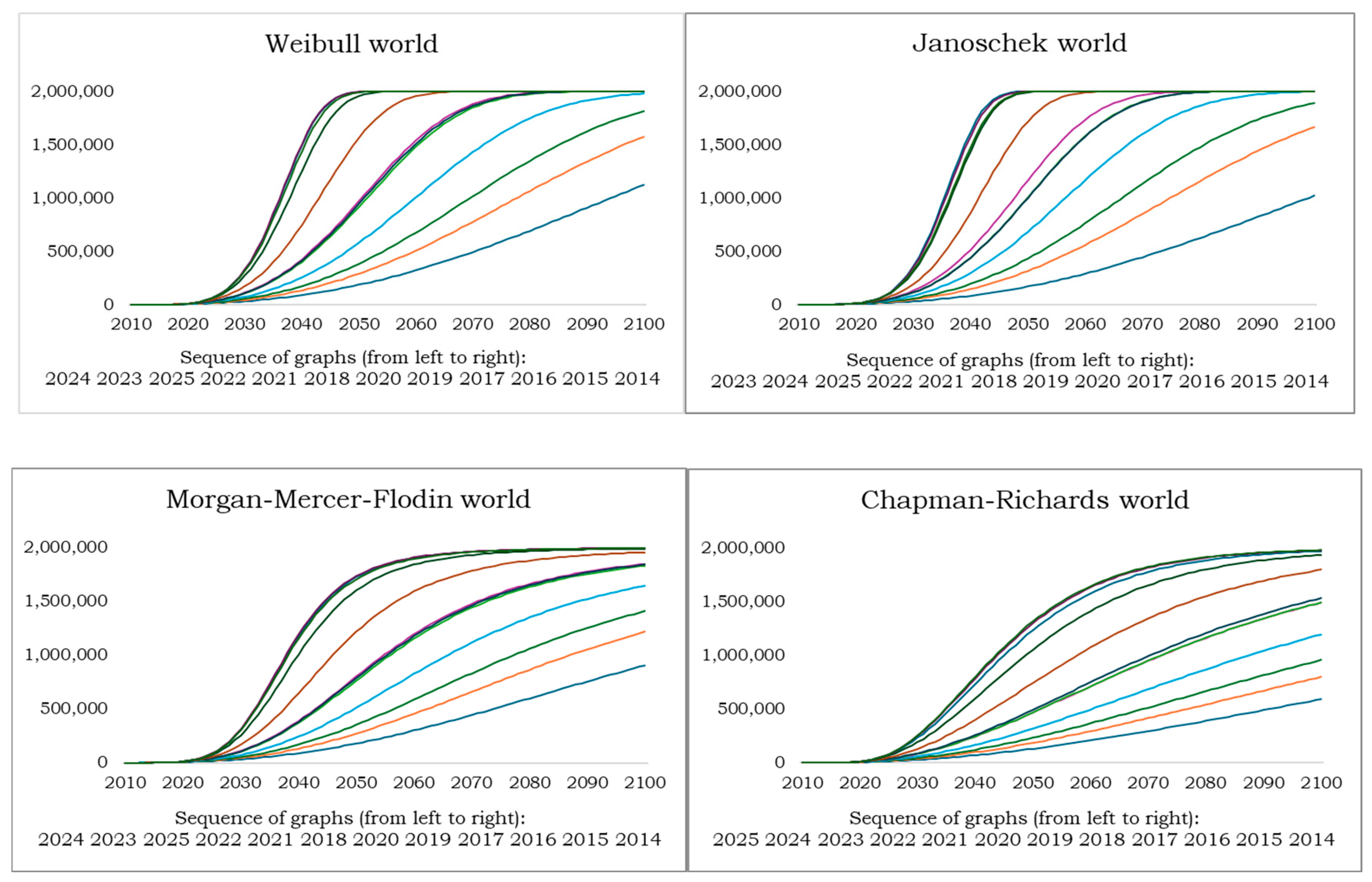
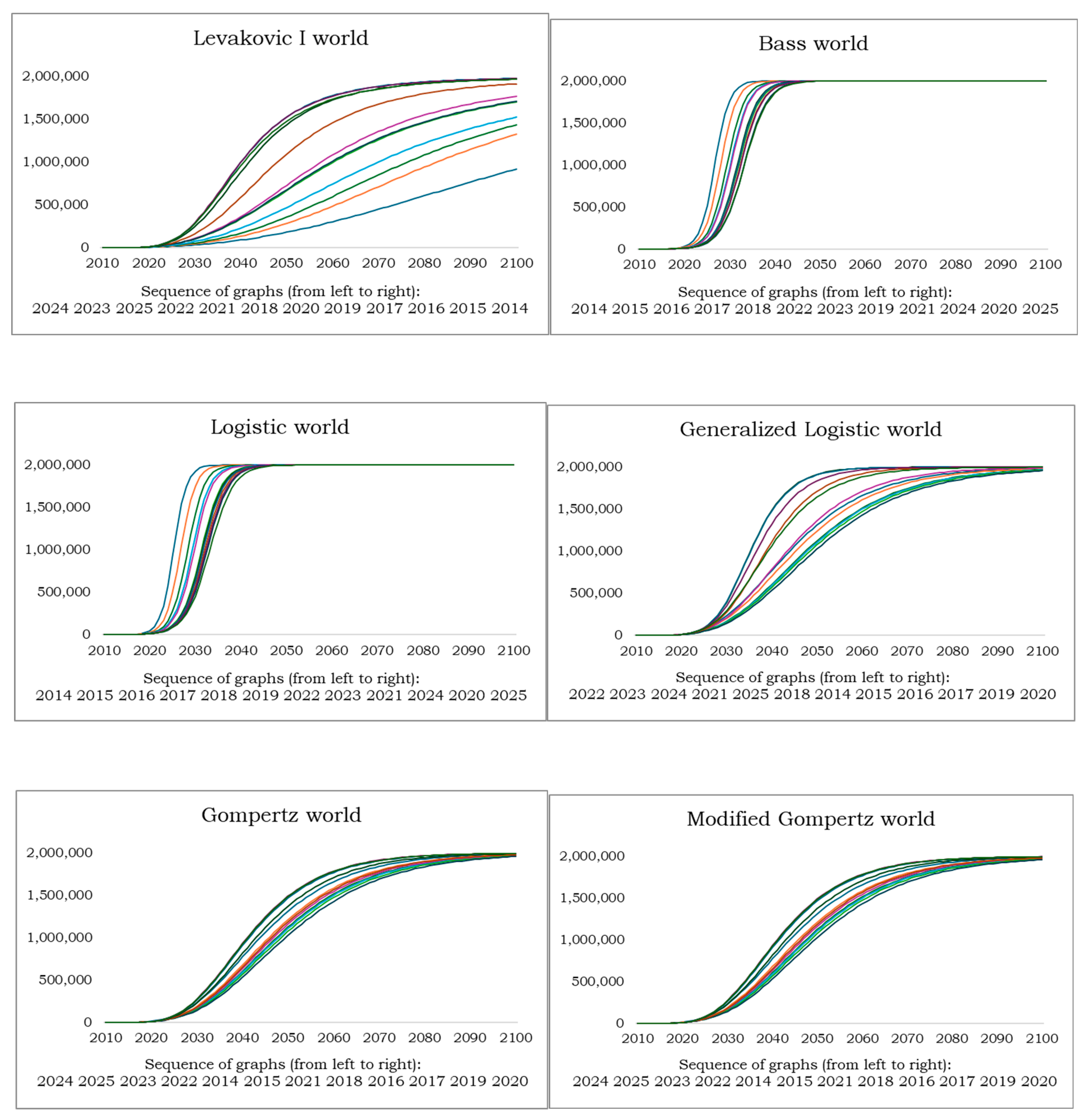

Table A1.
World: Inventory forecast for 2025 (thsds.), inflection and maximum acceleration points as of forecasts from 2014 to 2025.
Table A1.
World: Inventory forecast for 2025 (thsds.), inflection and maximum acceleration points as of forecasts from 2014 to 2025.
| Forecast for 2025 as of the end of … | 2014 | 2015 | 2016 | 2017 | 2018 | 2019 | 2020 | 2021 | 2022 | 2023 | 2024 | 2025 |
| Weibull | 16,020 | 20,997 | 24,821 | 31,540 | 42,901 | 41,494 | 42,149 | 57,154 | 75,404 | 83,784 | 84,226 | 82,513 |
| Janoschek | 15,164 | 21,983 | 26,305 | 34,083 | 47,230 | 43,125 | 43,066 | 60,337 | 79,917 | 86,441 | 85,131 | 82,667 |
| Morgan–Mercer–Flodin | 15,964 | 20,904 | 24,698 | 31,350 | 42,565 | 41,218 | 41,903 | 56,729 | 74,760 | 83,204 | 83,901 | 82,442 |
| Chapman–Richards | 14,613 | 18,840 | 22,214 | 27,884 | 37,125 | 37,180 | 38,582 | 51,359 | 67,540 | 77,395 | 80,863 | 81,664 |
| Levakovic I | 15,977 | 21,000 | 24,733 | 31,012 | 42,052 | 40,576 | 41,317 | 56,060 | 73,536 | 81,810 | 83,090 | 82,242 |
| Bass | 515,569 | 312,966 | 191,415 | 153,260 | 146,815 | 98,166 | 77,396 | 89,871 | 101,331 | 98,900 | 90,867 | 83,968 |
| Logistic | 904,660 | 486,706 | 267,815 | 191,020 | 166,577 | 109,436 | 84,062 | 93,021 | 102,573 | 99,491 | 91,185 | 84,088 |
| Generalized logistic | 79,069 | 67,487 | 56,525 | 55,097 | 67,270 | 53,056 | 49,942 | 72,326 | 89,404 | 90,821 | 86,402 | 82,612 |
| Gompertz | 79,042 | 65,846 | 56,505 | 55,083 | 59,752 | 53,045 | 49,939 | 60,092 | 73,372 | 80,755 | 82,498 | 82,123 |
| Modified Gompertz | 79,042 | 65,846 | 56,505 | 55,083 | 59,752 | 53,045 | 49,939 | 60,092 | 73,372 | 80,755 | 82,498 | 82,123 |
| Year with inflection point as of the end of … | 2014 | 2015 | 2016 | 2017 | 2018 | 2019 | 2020 | 2021 | 2022 | 2023 | 2024 | 2025 |
| Weibull | 2091 | 2076 | 2069 | 2060 | 2051 | 2052 | 2051 | 2044 | 2039 | 2037 | 2037 | 2037 |
| Janoschek | 2095 | 2074 | 2066 | 2057 | 2048 | 2050 | 2051 | 2042 | 2037 | 2036 | 2036 | 2037 |
| Morgan–Mercer–Flodin | 2082 | 2070 | 2063 | 2056 | 2048 | 2049 | 2049 | 2042 | 2037 | 2036 | 2036 | 2036 |
| Chapman–Richards | 2098 | 2084 | 2076 | 2066 | 2057 | 2057 | 2056 | 2048 | 2042 | 2039 | 2038 | 2038 |
| Levakovic I | 2082 | 2070 | 2063 | 2056 | 2049 | 2049 | 2049 | 2042 | 2038 | 2036 | 2036 | 2036 |
| Bass | 2027 | 2028 | 2029 | 2030 | 2030 | 2032 | 2033 | 2032 | 2032 | 2032 | 2032 | 2033 |
| Logistic | 2025 | 2027 | 2028 | 2029 | 2030 | 2031 | 2033 | 2032 | 2032 | 2032 | 2032 | 2033 |
| Generalized logistic | 2039 | 2041 | 2042 | 2043 | 2040 | 2043 | 2044 | 2037 | 2034 | 2034 | 2035 | 2036 |
| Gompertz | 2039 | 2041 | 2042 | 2043 | 2042 | 2043 | 2044 | 2041 | 2039 | 2037 | 2037 | 2037 |
| Modified Gompertz | 2039 | 2041 | 2042 | 2043 | 2042 | 2043 | 2044 | 2041 | 2039 | 2037 | 2037 | 2037 |
| Year with max acceleration as of the end of … | 2014 | 2015 | 2016 | 2017 | 2018 | 2019 | 2020 | 2021 | 2022 | 2023 | 2024 | 2025 |
| Weibull | 2056 | 2052 | 2049 | 2045 | 2041 | 2042 | 2041 | 2038 | 2035 | 2034 | 2034 | 2034 |
| Janoschek | 2049 | 2044 | 2042 | 2039 | 2036 | 2037 | 2037 | 2033 | 2031 | 2031 | 2031 | 2031 |
| Morgan–Mercer–Flodin | 2040 | 2038 | 2037 | 2035 | 2033 | 2033 | 2033 | 2031 | 2029 | 2029 | 2029 | 2029 |
| Chapman–Richards | 2029 | 2029 | 2029 | 2029 | 2028 | 2028 | 2028 | 2027 | 2027 | 2026 | 2026 | 2026 |
| Levakovic I | 2041 | 2040 | 2037 | 2033 | 2032 | 2031 | 2031 | 2030 | 2029 | 2028 | 2028 | 2027 |
| Bass | 2025 | 2026 | 2027 | 2027 | 2028 | 2029 | 2030 | 2029 | 2029 | 2029 | 2029 | 2030 |
| Logistic | 2023 | 2025 | 2026 | 2027 | 2027 | 2028 | 2029 | 2029 | 2029 | 2029 | 2029 | 2030 |
| Generalized logistic | 2028 | 2028 | 2029 | 2029 | 2029 | 2030 | 2030 | 2029 | 2028 | 2028 | 2028 | 2028 |
| Gompertz | 2028 | 2028 | 2029 | 2029 | 2029 | 2030 | 2030 | 2029 | 2028 | 2027 | 2027 | 2027 |
| Modified Gompertz | 2028 | 2028 | 2029 | 2029 | 2029 | 2030 | 2030 | 2029 | 2028 | 2027 | 2027 | 2027 |
Table A2.
Germany: Inventory forecast for 2025 (thsds.), inflection and maximum acceleration points as of forecasts from 2014 to -2025.
Table A2.
Germany: Inventory forecast for 2025 (thsds.), inflection and maximum acceleration points as of forecasts from 2014 to -2025.
| Forecast for 2025 as of the end of … | 2014 | 2015 | 2016 | 2017 | 2018 | 2019 | 2020 | 2021 | 2022 | 2023 | 2024 | 2025 |
| Weibull | 597 | 1,010 | 928 | 1,427 | 1,584 | 1,832 | 6,254 | 10,186 | 8,497 | 6,302 | 5,073 | 4,647 |
| Janoschek | 551 | 1,126 | 951 | 1,585 | 1,692 | 1,936 | 7,928 | 11,425 | 8,726 | 6,279 | 5,033 | 4,630 |
| Morgan–Mercer–Flodin | 593 | 1,001 | 920 | 1,410 | 1,564 | 1,807 | 5,944 | 9,445 | 8,088 | 6,160 | 5,029 | 4,639 |
| Chapman–Richards | 535 | 857 | 819 | 1,202 | 1,354 | 1,576 | 4,240 | 6,790 | 6,656 | 5,653 | 4,880 | 4,606 |
| Levakovic I | 597 | 1,010 | 923 | 1,387 | 1,534 | 1,770 | 5,455 | 7,954 | 7,148 | 5,390 | 4,743 | 4,560 |
| Bass | 16,285 | 14,616 | 6,428 | 6,904 | 5,061 | 4,329 | 11,672 | 14,498 | 10,665 | 7,217 | 5,420 | 4,736 |
| Logistic | 26,077 | 19,643 | 8,987 | 8,237 | 5,788 | 4,735 | 11,709 | 14,506 | 10,687 | 7,253 | 5,457 | 4,756 |
| Generalized logistic | 2,611 | 2,612 | 1,946 | 2,192 | 1,953 | 2,145 | 4,739 | 7,117 | 6,883 | 5,810 | 4,946 | 4,667 |
| Gompertz | 2,611 | 2,611 | 1,945 | 2,193 | 2,098 | 2,146 | 4,739 | 7,117 | 6,883 | 5,808 | 4,973 | 4,644 |
| Modified Gompertz | 2,611 | 2,611 | 1,945 | 2,193 | 2,098 | 2,146 | 4,739 | 7,117 | 6,883 | 5,808 | 4,973 | 4,644 |
| Year with inflection point as of the end of … | 2014 | 2015 | 2016 | 2017 | 2018 | 2019 | 2020 | 2021 | 2022 | 2023 | 2024 | 2025 |
| Weibull | 2078 | 2058 | 2060 | 2049 | 2046 | 2043 | 2030 | 2028 | 2029 | 2031 | 2033 | 2034 |
| Janoschek | 2083 | 2054 | 2059 | 2046 | 2045 | 2042 | 2029 | 2027 | 2029 | 2031 | 2033 | 2034 |
| Morgan–Mercer–Flodin | 2070 | 2053 | 2056 | 2046 | 2044 | 2041 | 2030 | 2027 | 2028 | 2030 | 2031 | 2032 |
| Chapman–Richards | 2083 | 2063 | 2065 | 2053 | 2050 | 2047 | 2033 | 2029 | 2029 | 2031 | 2032 | 2033 |
| Levakovic I | 2070 | 2053 | 2056 | 2046 | 2044 | 2041 | 2030 | 2028 | 2028 | 2029 | 2029 | 2030 |
| Bass | 2026 | 2026 | 2029 | 2028 | 2029 | 2030 | 2027 | 2026 | 2027 | 2029 | 2030 | 2031 |
| Logistic | 2025 | 2025 | 2028 | 2028 | 2029 | 2030 | 2027 | 2026 | 2027 | 2028 | 2030 | 2031 |
| Generalized logistic | 2037 | 2037 | 2040 | 2039 | 2041 | 2039 | 2032 | 2029 | 2029 | 2030 | 2032 | 2033 |
| Gompertz | 2037 | 2037 | 2040 | 2039 | 2039 | 2039 | 2032 | 2029 | 2029 | 2030 | 2032 | 2033 |
| Modified Gompertz | 2037 | 2037 | 2040 | 2039 | 2039 | 2039 | 2032 | 2029 | 2029 | 2030 | 2032 | 2033 |
| Year with max acceleration as of the end of … | 2014 | 2015 | 2016 | 2017 | 2018 | 2019 | 2020 | 2021 | 2022 | 2023 | 2024 | 2025 |
| Weibull | 2048 | 2042 | 2043 | 2038 | 2037 | 2036 | 2028 | 2027 | 2027 | 2028 | 2029 | 2030 |
| Janoschek | 2042 | 2036 | 2037 | 2033 | 2033 | 2032 | 2026 | 2025 | 2025 | 2026 | 2027 | 2027 |
| Morgan–Mercer–Flodin | 2034 | 2032 | 2032 | 2030 | 2030 | 2029 | 2025 | 2024 | 2024 | 2025 | 2025 | 2025 |
| Chapman–Richards | 2025 | 2026 | 2026 | 2025 | 2025 | 2025 | 2023 | 2022 | 2023 | 2023 | 2023 | 2023 |
| Levakovic I | 2037 | 2033 | 2033 | 2029 | 2028 | 2028 | 2024 | 2023 | 2023 | 2021 | 2021 | 2020 |
| Bass | 2024 | 2024 | 2026 | 2026 | 2027 | 2027 | 2025 | 2024 | 2025 | 2026 | 2027 | 2027 |
| Logistic | 2023 | 2023 | 2025 | 2025 | 2026 | 2027 | 2025 | 2024 | 2025 | 2026 | 2027 | 2027 |
| Generalized logistic | 2026 | 2026 | 2027 | 2027 | 2027 | 2027 | 2024 | 2023 | 2023 | 2023 | 2024 | 2024 |
| Gompertz | 2026 | 2026 | 2027 | 2027 | 2027 | 2027 | 2024 | 2023 | 2023 | 2023 | 2024 | 2024 |
| Modified Gompertz | 2026 | 2026 | 2027 | 2027 | 2027 | 2027 | 2024 | 2023 | 2023 | 2023 | 2024 | 2024 |
| 1 | The official figures for Germany (Kraftfahrt-Bundesamt [KBA] Germany, 2026) [59] could not be used because EV sales have only been reported since 2017. In addition, the vehicle types changed in the meantime. |
| 2 | The figures were calculated by adding up sales. Scrappage was not considered. Due to low sales figures in the early years, this was unlikely to have a significant impact. |
| 3 | Modified Gompertz = . Set , which is the original Gompertz function. |
| 4 | |
| 5 | A supplemental spreadsheet is available for better understanding. |
References
- United Nations Economic Commission for Europe. Electric vehicles and their potential to realize the sustainable development agenda. United Nations iLibrary. 2025. Available online: https://www.un-ilibrary.org/content/books/9789211066883c007.
- EV-Volumes, “EV-Volumes.”. Available online: https://ev-volumes.com/.
- United Nations. Paris Agreement. [CrossRef]
- IEA International Energy Agency. Net Zero Roadmap: A Global Pathway to Keep the 1.5 °C Goal in Reach. 2023, pp. 1–226. Available online: https://www.iea.org/reports/net-zero-roadmap-a-global-pathway-to-keep-the-15-0c-goal-in-reach.
- Shamsuddoha, M.; Tasnuba, N. The Road Ahead for Hybrid or Electric Vehicles in Developing Countries: Market Growth, Infrastructure, and Policy Needs 2025, 1–26. [CrossRef]
- Han, G.; Li, Z. A Structured Review of Electric Vehicle Sales Research: Multi-Level Driving Factors and Forecasting Pathways over the Past Decade. 2026, vol. 17(no. 122), 1–39. [Google Scholar]
- Lieven, T.; Mühlmeier, S.; Henkel, S.; Waller, J. F. Who will buy electric cars? An empirical study in Germany. Transp. Res. Part D. Transp. Environ. 2011, vol. 16(no. 3), 236–243. [Google Scholar] [CrossRef]
- Sierzchula, W.; Bakker, S.; Maat, K.; Van Wee, B. The influence of financial incentives and other socio-economic factors on electric vehicle adoption. Energy Policy 2014, vol. 68, 183–194. [Google Scholar] [CrossRef]
- Srinivasan, B. Predicting Future Electric Vehicle (EV) Sales: A Time Series Forecasting Approach Using Historical EV Sales Data. Int. J. Appl. Inf. Manag. vol. 5(no. 3), 177–189, 2025. Available online: https://ijaim.net/journal/index.php/ijaim/article/view/106. [CrossRef]
- Gnann, T.; Stephens, T. S.; Lin, Z.; Plötz, P.; Liu, C.; Brokate, J. What Drives the Market for Plug-In Electric Vehicles? -- A Review of International PEV Market Diffusion Models. Renew. Sustain. Energy Rev. 2018, vol. 93, 158–164. [Google Scholar] [CrossRef]
- Aalen, O.; Røysland, K.; Gran, J. M.; Ledergerber, B. Causality, Mediation and Time: A Dynamic Viewpoint. J. R. Stat. Soc. Ser. A (Stat. Soc. 2012, vol. 175(no. 4), 831–861. [Google Scholar] [CrossRef] [PubMed]
- Malthus, T. R. An Essay on the Principle of Population; J. Johnson: London, 1798. [Google Scholar]
- Rietmann, N.; Hügler, B.; Lieven, T. Forecasting the trajectory of electric vehicle sales and the consequences for worldwide CO2 emissions. J. Clean. Prod. 2020, vol. 261, 1–16. [Google Scholar] [CrossRef]
- Zeide, B. Analysis of Growth Equations. For. Sci. 1993, vol. 39(no. 3), 594–616. [Google Scholar] [CrossRef]
- A. Goriely, The Mathematics and Mechanics of Biological Growth, vol. 45. in Interdisciplinary Applied Mathematics; Springer, 2017; vol. 45.
- Monod, J. The Growth of Bacterial Cultures. Annu. Rev. Microbiol. 1949, vol. 3, 371–394. [Google Scholar] [CrossRef]
- West, G. B.; Brown, J. H.; Enquist, B. J. A General Model for the Origin of Allometric Scaling Laws in Biology. Science (80-. ) . 1997, vol. 276(no. 5309), 122–126. [Google Scholar] [CrossRef] [PubMed]
- Murray, J. D. Mathematical Biology I: An Introduction, 3rd ed.; Springer, 2002. [Google Scholar]
- Murray, J. D. Mathematical Biology II: Spatial Models and Biomedical Applications, 3rd ed.; Springer, 2003. [Google Scholar]
- Hunt, R. Plant Growth Curves: The Functional Approach to Plant Growth Analysis. In Edward Arnold; 1982. [Google Scholar]
- Hunt, R. Basic Growth Analysis: Plant Growth Analysis for Beginners; Unwin Hyman, 1990. [Google Scholar]
- Evans, L. T. The Quantitative Analysis of Plant Growth; University of California Press, 1972. [Google Scholar]
- Kermack, W. O.; McKendrick, A. G. A Contribution to the Mathematical Theory of Epidemics. Proc. R. Soc. A 1927, vol. 115(no. 772), 700–721. [Google Scholar] [CrossRef]
- Keeling, M. J.; Rohani, P. Modeling Infectious Diseases in Humans and Animals; Princeton University Press, 2008. [Google Scholar]
- Viboud, C.; Simonsen, L.; Chowell, G. A Generalized-Growth Model to Characterize the Early Ascending Phase of Infectious Disease Outbreaks. Epidemics 2016, vol. 15, 27–37. [Google Scholar] [CrossRef] [PubMed]
- Laird, A. K. Dynamics of Tumor Growth. Br. J. Cancer 1964, vol. 18, 490–502. [Google Scholar] [CrossRef] [PubMed]
- Solow, R. M. A Contribution to the Theory of Economic Growth. Q. J. Econ. 1956, vol. 70(no. 1), 65–94. [Google Scholar] [CrossRef]
- Swan, T. W. Economic Growth and Capital Accumulation. Econ. Rec. 1956, vol. 32(no. 2), 334–361. [Google Scholar] [CrossRef]
- Barro, R. J.; Sala-i-Martin, X. Economic Growth; McGraw-Hill, 1995. [Google Scholar]
- Mankiw, N. G.; Romer, D.; Weil, D. N. A Contribution to the Empirics of Economic Growth. Q. J. Econ. 1992, vol. 107(no. 2), 407–437. [Google Scholar] [CrossRef] [PubMed]
- Gompertz, B. On the Nature of the Function Expressive of the Law of Human Mortality. Philos. Trans. R. Soc. Lond. vol. 115, 513–583, 1825. [CrossRef]
- Verhulst, P. F. Notice sur la loi que la population poursuit dans son accroissement. Corresp. Mathématique Phys. vol. 10, 113–121, 1838.
- Bacaër, N. Verhulst and the logistic equation (1838). In A short history of mathematical population dynamics; Springer: London, 2011; Volume no. 1838 ch. 6, pp. 35–39. [Google Scholar] [CrossRef]
- Richards, F. J. A Flexible Growth Function for Empirical Use. J. Exp. Bot. 1959, vol. 10(no. 2), 290–301. [Google Scholar] [CrossRef]
- Tjørve, E.; Tjørve, K. M. C. A Unified Approach to the Richards Model Family for Use in Growth Analyses. J. Theor. Biol. 2010, vol. 267(no. 3), 417–425. [Google Scholar] [CrossRef] [PubMed]
- Tjørve, K. M. C.; Tjørve, E. The use of Gompertz models in growth analyses, and new Gompertz-model approach: An addition to the Unified-Richards family. PLoS ONE 2017, vol. 12(no. 6), 1–17. [Google Scholar] [CrossRef]
- Young, P. Technological growth curves. A competition of forecasting models. Technol. Forecast. Soc. Change 1993, vol. 44(no. 4), 375–389. [Google Scholar] [CrossRef]
- Zeide, B. Analysis of Growth Equations. For. Sci. 1993, vol. 39(no. 3), 594–616. [Google Scholar] [CrossRef]
- Buchanan, R. L.; Whiting, R. C.; Damert, W. C. When is simple good enough: a comparison of the Gompertz, Baranyi, and three-phase linear models for fitting bacterial growth curves. Food Microbiol. 1997, vol. 14(no. 4), 313–326. [Google Scholar] [CrossRef]
- Huo, H.; Wang, M. Modeling future vehicle sales and stock in China. Energy Policy 2012, vol. 43, 17–29. [Google Scholar] [CrossRef]
- Brdulak, A.; Chaberek, G.; Jagodziński, J. BASS Model Analysis in ``Crossing the Chasm’’ in E-Cars Innovation Diffusion Scenarios. Energies 2021, vol. 14(no. 11), 3216. [Google Scholar] [CrossRef]
- Rogers, E. M. Diffusion of Innovations, 5th ed.; Free Press: New, 2003. [Google Scholar]
- Fan, H.; Li, Z.; Duan, Y.; Wang, B. Incentive policy formulation for China’s electric vehicle market: Navigating pathways to sustainable mobility with a green premium analytical model. Energy Policy 2024, vol. 202, 114610, 2025. [Google Scholar] [CrossRef]
- Alatawneh, A.; Ghunaim, D. Towards vehicle electrification: A mathematical prediction of battery electric vehicle ownership growth, the case of Turkey. Green Energy Intell. Transp. 2024, vol. 3(no. 4), 100166. [Google Scholar] [CrossRef]
- Ayyadi, S.; Maaroufi, M. Diffusion models for predicting electric vehicles market in Morocco. In 2018 International Conference and Exposition on Electrical And Power Engineering (EPE); IEEE, 2018. [Google Scholar] [CrossRef]
- Dalkic-Melek, G.; Saltik, E. C.; Tuydes-Yaman, H. Electric Vehicle (EV) Market Penetration in Countries with Rising Motorization Rates. Int. J. Civ. Eng. 2025, vol. 23, 461–480. [Google Scholar] [CrossRef]
- Tang, B. jun; Wu, X. feng; Zhang, X. Modeling the CO2 emissions and energy saved from new energy vehicles based on the logistic-curve. Energy Policy 2013, vol. 57, 30–35. [Google Scholar] [CrossRef]
- Kumar, R. R.; Guha, P.; Chakraborty, A. Comparative assessment and selection of electric vehicle diffusion models: A global outlook. Energy 2022, vol. 238, 121932. [Google Scholar] [CrossRef]
- Lewis, C. D. Industrial and Business Forecasting Methods: A Practical Guide to Exponential Smoothing and Curve Fitting; Butterworth-Heinemann: Oxford, 1982. [Google Scholar]
- Weibull, W. A statistical distribution function of wide applicability. J. Appl. Mech. 1951, vol. 18(no. 3), 293–297. [Google Scholar] [CrossRef]
- Janoschek, A. Das reaktionskinetische Grundgesetz und seine Beziehungen zum Wachstums- und Ertragsgesetz. Stat. Vierteljahresschr. 1957, vol. 10, 25–37. [Google Scholar]
- Morgan, P. H.; Mercer, L. P.; Flodin, N. W. General Model for Nutritional Responses of Higher Organisms. Proc. Natl. Acad. Sci. 1975, vol. 72(no. 11), 4327–4331. [Google Scholar] [CrossRef] [PubMed]
- Levakovic, A. Growth functions in forest yield research. In Orig. Ger. Publ. For; journals, 1935. [Google Scholar]
- Bass, F. M. A New Product Growth Model for Consumer Durables. Manag. Sci. 1969, vol. 15(no. 5), 215–227. [Google Scholar] [CrossRef]
- Tsoularis, A.; Wallace, J. Analysis of Logistic Growth Models. Math. Biosci. 2002, vol. 179, 21–55. [Google Scholar] [CrossRef] [PubMed]
- Tofallis, C. A better measure of relative prediction accuracy for model selection and model estimation. J. Oper. Res. Soc. 2021, vol. 66(no. 8), 1352–1362. [Google Scholar]
- Moore, G. C.; Benbasat, I. Development of an instrument to measure the perceptions of adopting an information technology innovation. Inst. Manag. Sci. 1991, vol. 2(no. 3), 192–222. [Google Scholar] [CrossRef]
- Prospects 2050, “World Vehicle Forecasts & Strategies Propects 2050,” 2025. Available online: https://prospects-2050.com/wp-content/uploads/2025/04/World-Global-Prospects-2050.pdf.
- Kraftfahrt-Bundesamt (KBA) Germany. Monatliche Neuzulassungen (Monthly New Registrations). Available online: https://www.kba.de/DE/Statistik/Fahrzeuge/Neuzulassungen/MonatlicheNeuzulassungen/monatl_neuzulassungen_node.html (accessed on Dec. 31 2024).
Figure 1.
Growth function with four derivatives.
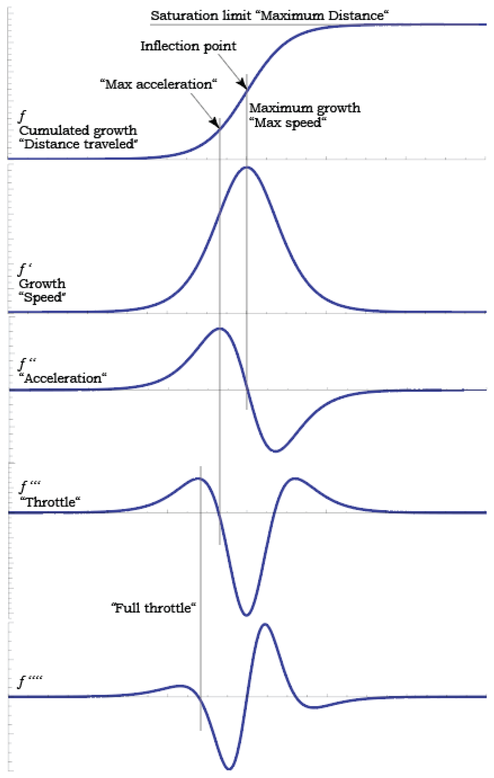
Figure 2.
Accumulated sales worldwide and in Germany, 2010–2025.
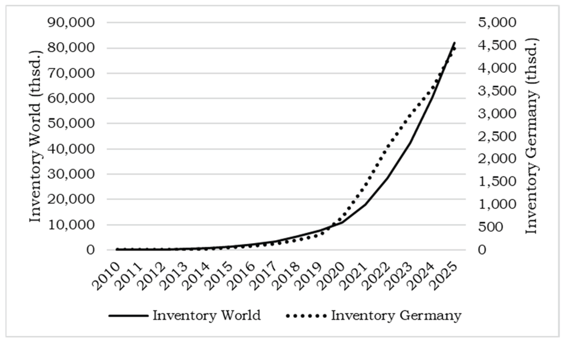
Figure 3.
Weibull function for world and Germany data with two datasets (2014 and 2025).
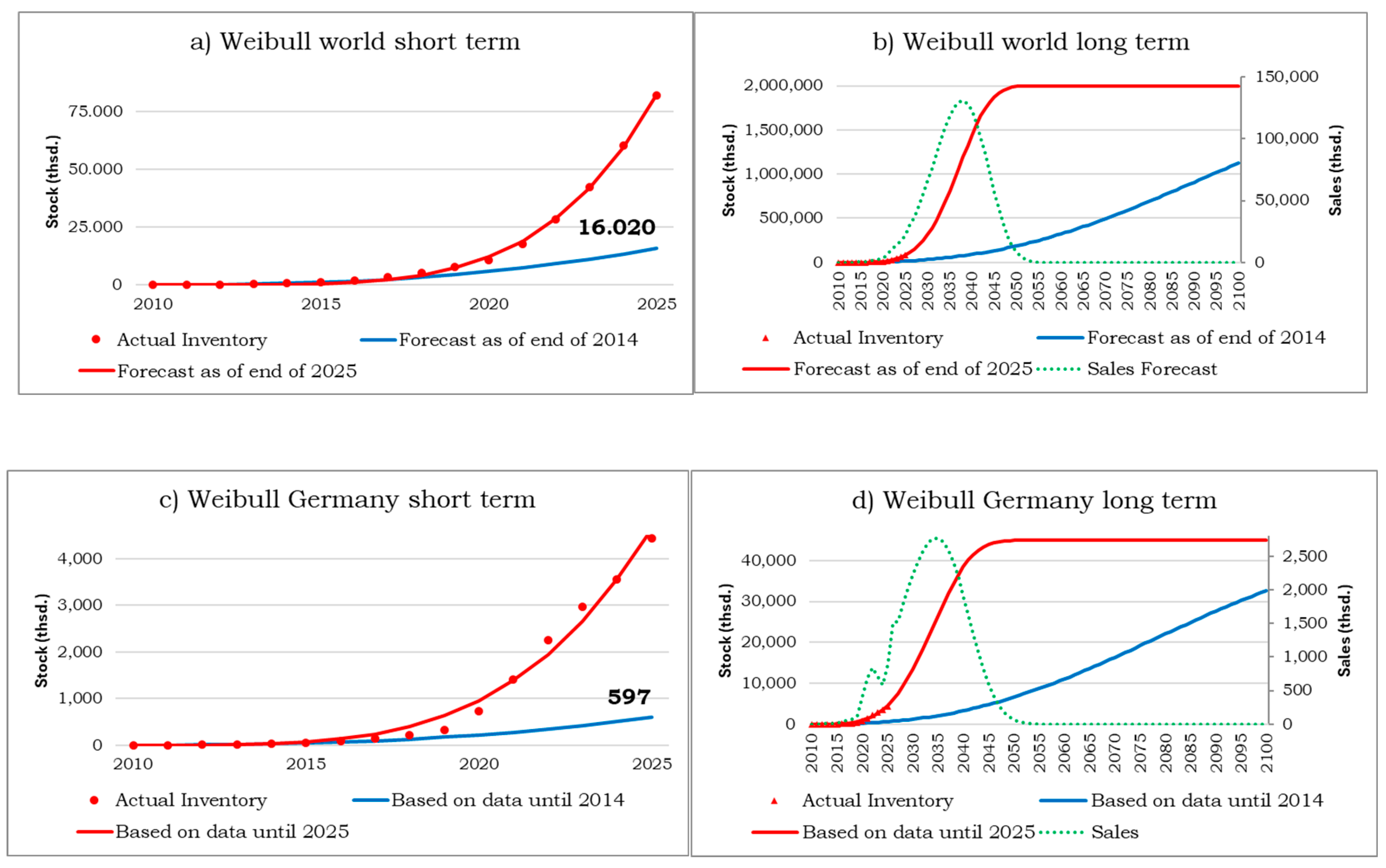
Figure 4.
Logistic function for world and Germany data with two datasets (2014 and 2025).
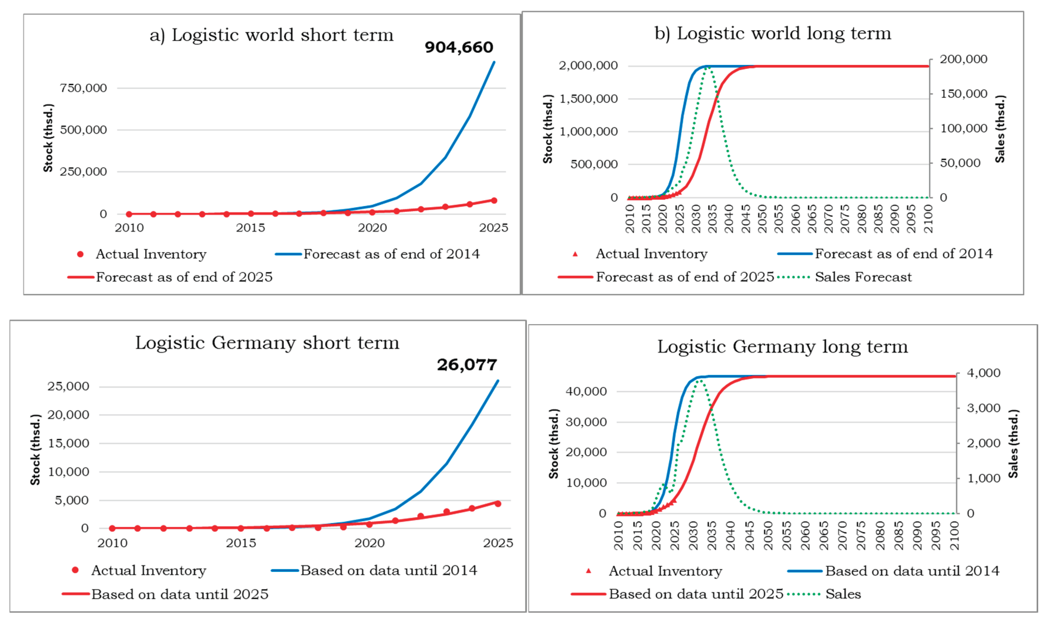
Figure 5.
Gompertz function for world and Germany data with two datasets (2014 and 2025).
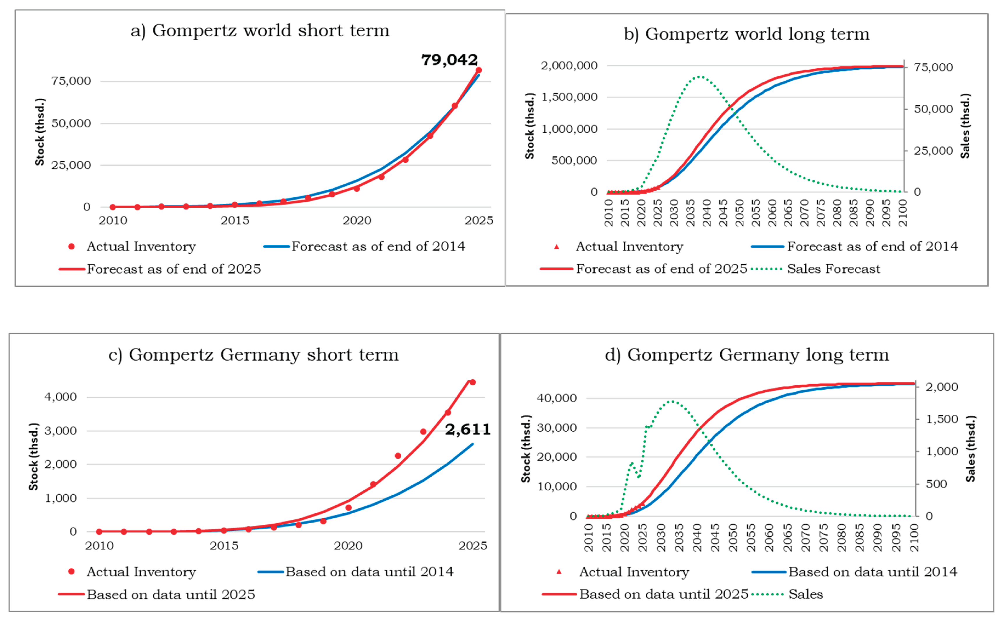
Figure 6.
Curve sets for three growth functions for forecasts as of the end of 2014 until 2025.
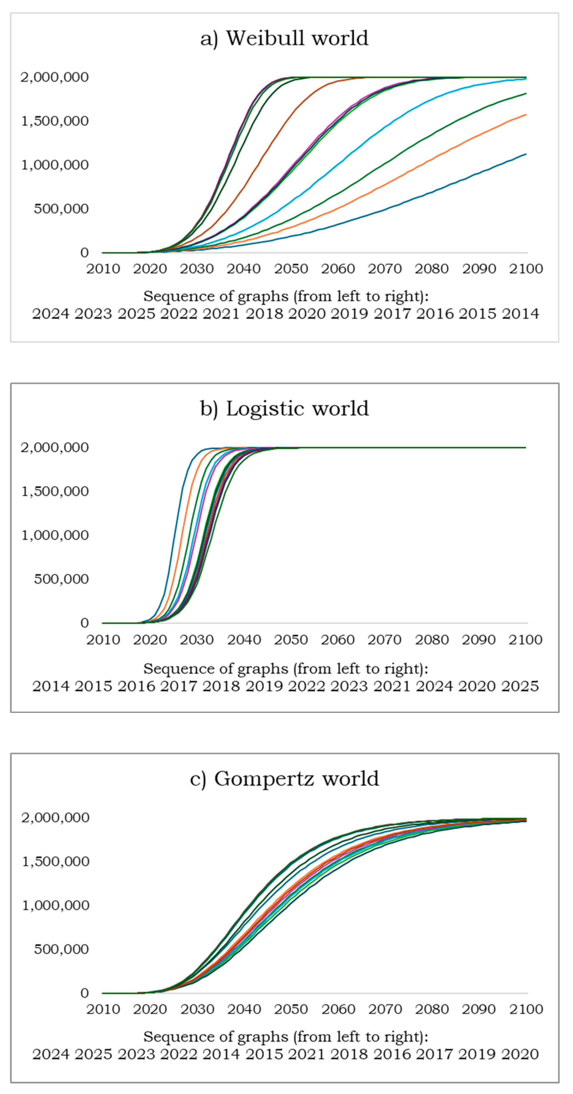
Figure 7.
Stocks until 2100 predicted with the Gompertz function as of the end of 2025.
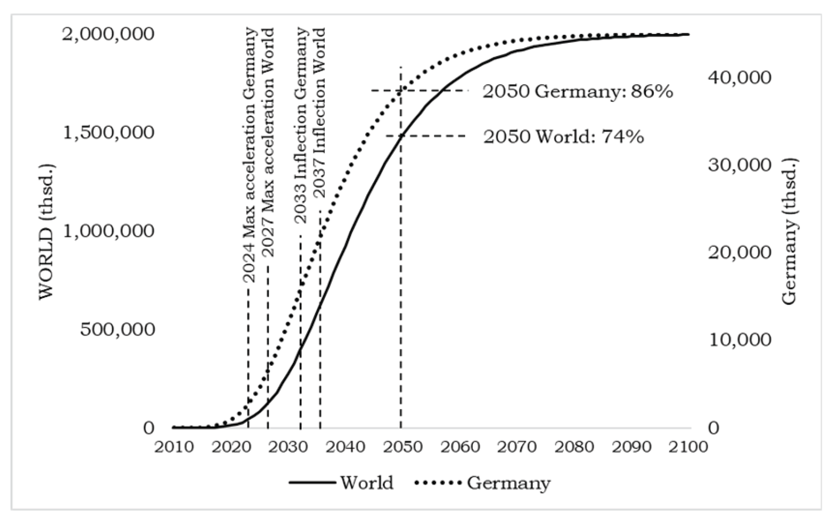
Table 1.
Accumulated sales worldwide and in Germany from 2010 until end-2025.
| Year | Inventory World (Thsds.) |
Inventory Germany (Thsds.) |
| 2010 | 6.455 | 0.144 |
| 2011 | 57.115 | 2.006 |
| 2012 | 189.391 | 8.294 |
| 2013 | 399.314 | 15.008 |
| 2014 | 723.111 | 28.288 |
| 2015 | 1,270.095 | 52.508 |
| 2016 | 2,067.732 | 80.617 |
| 2017 | 3,338.183 | 138.980 |
| 2018 | 5,428.178 | 211.568 |
| 2019 | 7,714.962 | 324.415 |
| 2020 | 10,973.599 | 724.881 |
| 2021 | 17,776.576 | 1,415.521 |
| 2022 | 28,339.720 | 2,258.320 |
| 2023 | 42,551.316 | 2,972.652 |
| 2024 | 60,351.368 | 3,556.524 |
| 2025 | 81,972.600 | 4,442.126 |
Table 2.
Growth functions used in this study.
| Distribution Function | Parameters | Max acceleration point (root of 3rd derivation) |
Inflection point (root of 2nd derivation) | |
| Weibull (1951) | M: Saturation limit l > 0: Scale parameter k > 0: Form parameter |
|||
| Janoschek (1957) | M: Saturation limit yo: Starting value at t = 0 m: Shape parameter |
|||
| Morgan–Mercer–Flodin Morgan et al. (1975) |
M: Saturation limit b: Scale along t d: Shape |
|||
| Chapman–Richards Richards (1959) |
M: Saturation limit k: Growth rate m: Shape |
|||
| Levakovic I Levakovic (1935); Zeide (1993) |
M: Saturation limit b: Horizontal position c: Shape d: Asymmetry parameter |
|||
| Bass (1969) | M: Saturation limit p: Coefficient of innovation q: Coefficient of imitation |
|||
| Logistic Verhulst (1838) |
M: Saturation limit r: Growth rate a: Constant |
|||
| Generalized logistic Richards (1959; Tsoularis and Wallace (2002) |
M: Saturation limit a: Changes horizontal position r: Growth rate n: Asymmetry parameter |
|||
| Gompertz (1825) | M: Saturation limit b: Changes horizontal position c: Growth rate |
|||
| Modified Gompertz | M: Saturation limit b: Inflection point g: Time scaling |
b |
Table 3.
Actual inventories and forecasts based on historic data until 2014 calculated using (5)4.
Table 3.
Actual inventories and forecasts based on historic data until 2014 calculated using (5)4.
| Adaptation Period | Prediction Period | |||||||||||||||
| Year | 2010 | 2011 | 2012 | 2013 | 2014 | 2015 | 2016 | 2017 | 2018 | 2019 | 2020 | 2021 | 2022 | 2023 | 2024 | 2025 |
| Actual Inventory | 6 | 57 | 189 | 399 | 723 | 1,270 | 2,068 | 3,338 | 5,428 | 7,715 | 10,974 | 17,777 | 28,340 | 42,551 | 60,351 | 81,973 |
| Forecast | 35 | 82 | 181 | 375 | 734 | 1,361 | 2,408 | 4,072 | 6,611 | 10,332 | 15,595 | 22,792 | 32,338 | 44,643 | 60,097 | 79,042 |
| Absolute percentage error | 441% | 44% | 4% | 6% | 1% | 7% | 16% | 22% | 22% | 34% | 42% | 28% | 14% | 5% | 0% | 4% |
Note: t = 1 for 2010; inventories in thsds, absolute percentage error = Abs(Forecast – Actual) / Actual.
Table 4.
Fit indices.
| a) World | Adaptation Process | Prediction Process | |||||
| Fit Indices | RMSE | AIC | MAPE | RMSE | AIC | MAPE | |
| Weibull | 548 | 1584 | 22.76% | 22720 | 1519 | 34.24% | |
| Janoschek | 441 | 1542 | 17.33% | 22062 | 1518 | 32.95% | |
| Morgan–Mercer–Flodin | 552 | 1585 | 22.98% | 22798 | 1520 | 34.36% | |
| Chapman–Richards | 704 | 1635 | 27.56% | 24245 | 1528 | 37.17% | |
| Levakovic I | 572 | 1595 | 23.68% | 22905 | 1522 | 34.52% | |
| Bass | 564 | 1590 | 13.60% | 76702 | 1680 | 70.08% | |
| Logistic | 588 | 1598 | 20.22% | 144863 | 1764 | 124.88% | |
| Generalized logistic | 371 | 1507 | 8.09% | 9953 | 1412 | 15.09% | |
| Gompertz | 536 | 1579 | 17.52% | 10746 | 1421 | 16.00% | |
| Modified Gompertz | 536 | 1579 | 17.52% | 10746 | 1421 | 16.00% | |
| b) Germany | Adaptation Process | Prediction Process | |||||
| Fit Indices | RMSE | AIC | MAPE | RMSE | AIC | MAPE | |
| Weibull | 93 | 1222 | 30.80% | 1863 | 1189 | 50.71% | |
| Janoschek | 89 | 1215 | 50.35% | 1977 | 1199 | 51.85% | |
| Morgan–Mercer–Flodin | 90 | 1215 | 30.77% | 1803 | 1185 | 49.96% | |
| Chapman–Richards | 78 | 1185 | 34.94% | 1678 | 1175 | 48.49% | |
| Levakovic I | 66 | 1155 | 35.03% | 1681 | 1178 | 47.81% | |
| Bass | 121 | 1276 | 46.55% | 3083 | 1256 | 54.50% | |
| Logistic | 123 | 1282 | 54.58% | 4671 | 1313 | 80.57% | |
| Generalized logistic | 84 | 1204 | 28.24% | 1238 | 1137 | 34.41% | |
| Gompertz | 84 | 1202 | 28.26% | 1230 | 1134 | 34.27% | |
| Modified Gompertz | 84 | 1202 | 28.26% | 1230 | 1134 | 34.27% | |
Note: RMSE: Root mean square error; AIC: Akaike information criterion; MAPE: Mean absolute percentage error.
Table 5.
Fit indices for three functions with saturation limits of 2 and 3 billion EVs.
| Fit indices | RMSE | AIC | MAPE | RMSE | AIC | MAPE |
| Weibull 2 bn | 548 | 1584 | 22,76% | 22720 | 1519 | 34.24% |
| Weibull 3 bn | 547 | 1583 | 22,69% | 22694 | 1519 | 34.20% |
| Logistic 2 bn | 588 | 1598 | 20,22% | 144863 | 1764 | 124.88% |
| Logistic 3 bn | 601 | 1603 | 20,62% | 165626 | 1782 | 133.04% |
| Gompertz 2 bn | 536 | 1579 | 17,52% | 10746 | 1421 | 16.00% |
| Gompertz 3 bn | 505 | 1567 | 16,28% | 9732 | 1407 | 15.72% |
Note: RMSE: Root mean square error; AIC: Akaike information criterion; MAPE: Mean absolute percentage error.
Disclaimer/Publisher’s Note: The statements, opinions and data contained in all publications are solely those of the individual author(s) and contributor(s) and not of MDPI and/or the editor(s). MDPI and/or the editor(s) disclaim responsibility for any injury to people or property resulting from any ideas, methods, instructions or products referred to in the content. |
© 2026 by the authors. Licensee MDPI, Basel, Switzerland. This article is an open access article distributed under the terms and conditions of the Creative Commons Attribution (CC BY) license (http://creativecommons.org/licenses/by/4.0/).
Copyright: This open access article is published under a Creative Commons CC BY 4.0 license, which permit the free download, distribution, and reuse, provided that the author and preprint are cited in any reuse.