

Submitted:
13 June 2026
Posted:
15 June 2026
You are already at the latest version
Abstract
Oil extraction and agricultural production are central to North Dakota’s economy, yet their spatial coexistence and implications for sustainable land-use planning remain poorly understood. This study conducts a statewide geospatial analysis integrating OpenStreetMap data, GIS processing, DBSCAN clustering, and spatial statistics to examine the colocation of 7,102 oil well and 4,277 grain silo sites. Hotspot and spatial heterogeneity tests using the Getis–Ord Gi* statistic and local Moran’s I reveal a pronounced spatial divide: oil activity is tightly clustered in the western Bakken region, whereas grain storage facilities concentrate across central and eastern counties. The limited geographic overlap suggests minimal systemic land-use overlap, though localized high-intensity co-location patterns emerge in McKenzie, Dunn, and Mountrail counties. These patterns provide stakeholders with insight into locations where shared logistics pressures and land-use tensions may influence sustainable infrastructure planning. More broadly, the study demonstrates the value of spatial data mining techniques applied to free, publicly available data for identifying intersectoral infrastructure patterns that inform sustainable land-use, infrastructure, and regional development planning across North Dakota.
Keywords:
GIS
; sustainable land-use planning
; infrastructure co-location
; oil wells
; grain silos
; spatial analysis
; regional resilience
1. Introduction
Sustainable land-use planning, infrastructure resilience, and resource stewardship depend on understanding how multiple infrastructures coexist within shared geographic space. In resource-intensive regions, overlap between industrial and agricultural activities can influence transportation networks, environmental systems, land allocation, and long-term sustainability outcomes. North Dakota offers a clear case: rapid oil development associated with the Bakken formation has expanded alongside an established grain production system, creating counties where oil well sites and grain storage facilities are situated in close proximity. These co-located activities have the potential to increase competition for freight capacity, influence safety and environmental outcomes, and affect regional resilience during demand shocks.
During the 2013–2014 crude-by-rail surge, oil shipments displaced grain movements across the Upper Midwest, causing railcar shortages, wider basis levels, and higher storage pressures—clear indicators of constrained logistics capacity and shifting traffic [1,2]. These disruptions reduced producer revenues, raised operational risks, and complicated regional infrastructure coordination.
Despite the visible proximity of oil pads and grain silos on conventional maps, little is known about whether these sectors interact at spatial scales that meaningfully affect logistics performance, land use dynamics, or safety outcomes. Though there is existing research linking increased crude-by-rail volumes to agricultural bottlenecks particularly for [3], many studies rely on aggregated regional data or sector-specific analyses that overlook fine-scale cross-sector interactions. Consequently, planners and policymakers lack the localized empirical evidence needed to support sustainable infrastructure investment, land-use coordination, and long-term regional resilience.
The study aimed to identify statistically significant clusters where oil extraction and agricultural storage activities co-locate within spatial scales potentially relevant to operational interactions in North Dakota. To achieve this goal, the study developed a geospatial workflow using OpenStreetMap (OSM) because it provides consistent spatial geometries for both infrastructure types within a unified dataset. Unlike North Dakota Industrial Commission (NDIC) and United States Department of Agriculture (USDA) registries, OSM supplies polygon and line geometries needed to derive site centroids and aggregate co-located structures. The workflow unified operational sites through density-based clustering of mapped infrastructure footprints before applying spatial association techniques.
The contributions of this work are threefold. First, the study provides a framework for converting heterogeneous spatial features into operational units to strengthen spatial analysis and decision-making, with potential transferability to comparable data environments. Second, the analysis identifies statistically significant oil–agriculture co-location hotspots that may warrant further investigation for sustainable infrastructure and resource-management planning. Third, the study presents a spatial cluster-detection methodology adaptable to other regions and phenomena, with broader applications in land-use and logistics research. Collectively, these contributions advance the understanding of sectoral spatial relationships in a state’s evolving landscape and support evidence-based sustainability planning, supporting a data-driven approach to managing complex spatial relationships between energy and agriculture, with implications for safety, efficiency, and economic sustainability.
The sustainability relevance of this study arises from the need to manage multiple infrastructure systems within shared landscapes. Oil extraction and agricultural storage represent economically important but spatially competing land uses that can influence transportation demand, resource allocation, environmental conditions, and regional resilience. Identifying where these systems remain spatially separated and where they converge provides information that can support more sustainable land-use planning, infrastructure investment, and long-term regional development strategies.
The organization of the rest of this paper is as follows: Section 2 reviews the literature on energy-agriculture spatial interactions in North Dakota; Section 3 describes the geospatial workflow; Section 4 presents and interprets the results; Section 5 discusses implications and limitations; Section 6 concludes the study.
2. Literature Review
Since the early 2000s, rapid expansion of unconventional oil and gas development in North Dakota’s Bakken Shale has fundamentally transformed the state’s rural landscape. This expansion generated unprecedented conflicts between energy infrastructure and agricultural systems [4]. This energy boom, fueled by horizontal drilling and hydraulic fracturing technology, has industrialized traditional rural, agricultural counties in western North Dakota, resulting in complicated interactions between competing land uses [5]. The scale and intensity of this development make it a unique case study to understand how energy infrastructure interacts with established agricultural systems in rural America.
North Dakota’s shift from a predominantly agricultural state to a major oil producer reflects broader conflicts between traditional rural economies and extractive industries [6]. North Dakota now accounts for roughly 11% of American oil production, with rural regions such as Williams County facing fast in-migration of oilfield workers and acute infrastructure challenges [7]. This section examines how energy development affects agricultural infrastructure and related rural systems, drawing on empirical research that documented land-use changes, transportation disputes, resource competition, and socioeconomic impacts in North Dakota’s rural communities.
2.1. Direct Land Use Conflicts and Agricultural Displacement
Fitzgerald et al. (2020) found that drilling reduced crop cover and increased fallow land, with effects that were spatially and temporally heterogeneous across cropland classes and frequently temporary [4]. Many effects were temporary. This suggests that previous estimates have overvalued the net impact of drilling by as much as twice. Preston and Kim (2016) further quantified 12,990 hectares of land converted to well pads, primarily from agriculture (49.5%) and prairie (47.4%) [8]. Projected development is expected to affect 2.3% of the Bakken drilling landscape and adjacent grasslands. In addition, Alfred et al. (2015) referred to the infrastructure requirements of horizontal drilling and hydraulic fracturing as reducing large areas of the Great Plains into industrialized land [6]. This pattern reflects the broader transformation of agricultural landscapes driven by energy development.
Rakitan (2018) examined the economic repercussions of land displacement and its influence, particularly on surface rent in North Dakota [9]. The study revealed that surface tenants’ willingness to pay for land parcels near oil facilities had not changed significantly. This conclusion draws on approximately 17,000 land rental transactions obtained from State Trust Lands data. Although many scholars argue that energy development can reduce agricultural profitability, recent evidence shows that proximity to oil and gas activity is linked to measurable declines in agricultural output. Spatial analyses of unconventional oil and gas expansion consistently find reductions in crop acreage and increases in fallow land as drilling intensifies [10]. Similarly, studies in shale regions also reported farm-level adjustments including consolidation, altered production decisions, and reduced crop cover associated with drilling footprints [11]. Smith et al. (2019) further confirmed these patterns, highlighting recurring proximity effects such as land-use displacement and operational disruptions [12].
2.2. Transportation Infrastructure Competition and Damage
Energy expansion has resulted in fierce rivalry for transportation infrastructure, particularly in the transfer of agricultural commodities. Villegas (2016) examined how growing rail demand from the energy sector has impacted wheat transportation in the Upper Midwest [13]. In this region, rail service is the most cost-effective shipping option for agricultural commodities. As oil has taken up freight capacity on trains, farmers in regions like North Dakota have had to pay more to reach grain markets, resulting in financial losses. Similarly, Ortiz (2016) found that railroad congestion from energy development impaired wheat markets, creating price differentials across Midwest producers relative to Gulf Coast markets [13]. Historically, oil price declines exacerbated farmers’ shipping challenges as energy firms used railcars to store excess crude oil inventory. This further impeded agricultural access to transportation infrastructure.
Heavy truck traffic from energy development caused substantial damage to rural roads and bridges. A study by McCarthy et al. (2015) highlighted the economic effects on roads and bridges in multiple states, especially in North Dakota [14]. This finding indicates a need for infrastructure upgrades and new bridge construction to address increased traffic volumes. Furthermore, Dharmadhikari et al. (2016) reported on rural bridge construction needs in North Dakota [15]. They revealed that oil exploration escalates vehicle traffic and heightens maintenance demands on infrastructure.
Rahm et al. (2015) used comparative data from Texas to reveal alarming safety trends [16]. These included a 26% increase in crash rates and a 49% rise in fatalities and severe injuries, alongside deteriorating road conditions and escalating maintenance costs. While the Texas study emphasized a regional context, the pattern of infrastructure strain it documented—increased crash rates and maintenance costs—has been similarly reported in North Dakota counties experiencing high drilling activity [17].
2.3. Water Resource Competition and Management Challenges
Water resource competition represents a critical but often overlooked form of infrastructure interference. Horner et al. (2016) provided a comprehensive analysis of water use in the Bakken Shale and documented that water use for hydraulic fracturing grew five-fold, from 770 million gallons in 2008 to 4.3 billion gallons in 2012 [18]. The study found that existing groundwater resources are inadequate to meet hydraulic fracturing demand. This creates competition with agricultural water needs.
A study by Hearne & Fernando investigated water management strategies in North Dakota’s oil-producing region. They observed that while the Missouri River and Lake Sakakawea supply abundant water, infrastructure expansion during oil boom periods proved challenging [19]. Sales from drilling activities have helped support the building of regional water systems. This resulted in a complicated interdependence between agricultural and energy water infrastructure. Furthermore, Fernando & Cooley (2016) discovered that transportable on-site treatment facilities could be cost-effective while reducing competition for freshwater resources [20].
Smith and Haggerty (2020) studied how public infrastructure investments in water systems contain “exploitable ambiguities” that various stakeholders use to pursue divergent agendas [21]. Their research of a large regional water supply project demonstrated how infrastructure decisions in energy-dependent societies have confusing implications for agricultural customers.
2.4. Economic and Social Dimensions of Interference
Socioeconomic impacts of energy–agriculture interactions introduce complex challenges beyond land-use conflict alone. A framework by Fernando & Cooley (2016) identified five critical issues arising from oil booms: the need for affordable housing, improvements in community infrastructure, enhancement of public services, attraction of new businesses, and strategies for community integration [20]. These elements significantly influence the social dynamics and economic sustainability of agricultural communities.
Addey (2019) applied autoregressive distributed lag models to investigate the effects of the oil boom on North Dakota’s agricultural sector providing evidence that the oil industry adversely affected agriculture but did not significantly affect manufacturing [22]. The study recorded an 80% adjustment speed coefficient, indicating that imbalances may rectify themselves within approximately three months. Additionally, their study advocated for structural spending policies aimed at mitigating the negative influences on sectors competing for labor.
Recent studies indicate that the social effects of energy development are complex. They extend well beyond the physical structures associated with energy development, in a manner not captured by measures of distance alone. For instance, McGranahan et al. (2017) discovered that the observed effects of energy development are correlated to the affected area in a weak fashion [5]. The study revealed the importance of various social factors. These include views on development, compensation levels, and levels of disruption, as important considerations in community responses to energy development. A study of Williams County, North Dakota, found that the influx of energy development contributed to “rural gentrification” [7]. In this phenomenon, oil field employees, who are generally wealthier, displace the existing agricultural populations in the region. The study revealed instability of the social structures of the region, influenced by the associated markets of production.
2.5. Environmental and Ecological Interference
Environmental interference between energy and agricultural systems poses significant challenges for rural communities. A study by Spiess et al. (2020) explored the impact of fracking traffic on bird and invertebrate communities [23]. The study revealed that dust emissions led to substantial deposition 180 m into adjacent crop fields. While wildlife in agricultural landscapes displayed some resilience to these impacts, the findings highlighted the environmental pathways through which energy development can affect agricultural areas.
Boslett et al. (2021) documented increased light pollution associated with shale oil and gas development in rural regions [24]. Their analysis of nationwide data from 2000 to 2012 indicated strong correlations between increased drilling activities, insufficient sleep, and deteriorating health outcomes. These findings highlighted a quality-of-life interference that adversely affects agricultural communities. Additionally, Van der Burg et al. (2023) examined the responses of grassland bird populations to the expansion of energy portfolios [25]. Their findings indicated that birds reacted more negatively to biofuel feedstocks, particularly corn and soybeans, compared to oil and gas development. This research suggested that renewable energy policies encouraging biofuel production may inadvertently create broader ecological disruptions within grassland systems than fossil fuel extraction. This is because both forms of energy development contribute to shifts in wildlife population distributions.
2.6. Policy Responses and Mitigation Strategies
Many studies have examined governance responses and mitigation measures addressing energy–agriculture conflicts. For instance, Smith et al. (2019) examined the community reactions towards the adaptation of shared services for dealing with service crises during the energy boom [12]. They found that although the innovations have demonstrated resourcefulness for the communities, they have triggered unrealistic boom periods and contributed towards the development of potentially unsustainably operating projects.
Fernando and Goreham (2018) examined the community capital perspectives in two different rural cities [26]. They discussed the optimization of social capital investment, identification of cultural capital alterations, and the utilization of political capital for effectively dealing with boom effects. In related work using predictive modeling tools to aid transportation infrastructure planning in areas experiencing rapid energy expansion, Lee et al. (2021) demonstrated that by adapting the susceptible-infected-recovered (SIR) epidemic framework, drilling locations with significant traffic implications can be forecasted ahead of time [27]. Forecasting allows transportation agencies to better anticipate and mitigate emerging infrastructure conflicts.
Overall, the literature on energy development and agricultural infrastructure in North Dakota reveals pressures that extend beyond simple land-displacement impacts. Impacts vary in time and space, with some disruptions being short and others lasting. Energy-related traffic impedes agricultural product movement, posing logistical issues. As the competition for resources like water grows, agricultural operations become strained. Economic research yields conflicting results on land rental values and productivity losses. However, the social consequences, such as housing relocation and demographic shifts, are more visible. These changes suggest that energy growth fundamentally alters rural systems through interwoven infrastructural, economic, and social dynamics.
To the authors’ knowledge, no prior study has examined oil–agriculture spatial relationships at the site level using an open-data geospatial workflow that enables statistical detection of fine-scale co-location patterns across North Dakota. This gap motivates the present analysis.
3. Materials and Methods
The study conducted all spatial data processing and analysis in Python within a transferrable computational workflow. The study obtained and preprocessed OSM data externally as GeoPackage (GPKG) files and imported them into the Python environment. The GeoPandas library performed spatial data manipulation, including coordinate transformation and geometric operations. The study clustered oil well and silo features using the DBSCAN algorithm from the scikit-learn library.
Spatial weights for local and global statistics were constructed using the DistanceBand class from the PySAL (libpysal) library, with row-standardization applied. Bivariate spatial autocorrelation was computed using PySAL’s esda package, specifically the Moran_BV (global) and Moran_Local_BV (local) implementations. Statistical significance was assessed using 999 Monte Carlo permutations for both global and local Moran’s I statistics. All analyses were conducted in a Python environment using standard scientific computing libraries, including NumPy and Pandas, with visualization and mapping performed using Matplotlib and GeoPandas. Figure 1 illustrates this study’s workflow with the procedures, as coded in software.
3.1. Data Source
All spatial operations were conducted using a projected coordinate reference system (CRS), specifically NAD83/UTM Zone 14N (EPSG:26914). This projection preserves spatial relationships in metric units and is appropriate for distance-based analyses such as DBSCAN clustering and neighborhood definition. All distance thresholds were computed directly in meters within this projected coordinate system. Degree-based equivalents are reported only for reference. “Well sites” and “silo sites” refer to DBSCAN-derived site centroids representing aggregated groups of spatially proximate features. OSM was selected as the primary data source because the workflow required spatial geometries of infrastructure footprints, whereas NDIC and USDA datasets primarily function as attribute registries. Individual “wells” and “silos” refer to the underlying OSM features contained within each site. The following OSM searches retrieved site data for oil wells:
KEY ‘industrial’ = ‘oil’ IN ‘North Dakota’
KEY ‘man made’ = ‘petroleum well’ IN ‘North Dakota’
Table 1 summarizes the results of the search for oil wells in North Dakota. The search returned polygons that reflect the outline of oil pads. A GIS procedure converted the polygons to centroids objects for points-based spatial analysis. Another GIS procedure merged 5640 well pad centroids and 7315 well points to produce a total of 12,955 well points. Guided by a threshold sensitivity analysis, the DBSCAN algorithm applied a 200-m (0.002-degree) threshold to form 7102 well sites. Each site contained a number of well points.
To simplify the analysis, the study did not apply explicit deduplication of well pad centroids and well point features, because DBSCAN aggregated proximate features into clusters based on the predetermined distance threshold. Cluster size, defined as the number of OSM features aggregated within each DBSCAN site, served as the spatial intensity attribute for Gi* and Moran’s I. This metric reflects the density of mapped features per site and may overcount facilities with multiple OSM representations (e.g., a single elevator mapped as both a polygon and a point); this limitation is acknowledged in the sensitivity analysis.
Figure 2 shows an example of the two cases of cluster centroid labeling: 1) the centroid of a well site containing a well pad with no wells, and 2) the centroid of a well site containing wells on two nearby well pads. Hence, this example shows two well sites with one containing no wells (left) and the other (right) containing a total of 12 well points on two nearby well pads.
Although not detected through multiple random inspections, this approach introduced a potential risk of pseudo-replication where the same physical site could be counted multiple times if positional inaccuracies placed features outside the threshold, or merged into a single cluster if features fell within it. These effects are inherent in using heterogeneous OSM data and are acknowledged as a limitation.
The study established silo sites using the same clustering approach applied to well sites. The OSM search used:
KEY ‘man made’ = ‘silo’ IN ‘North Dakota’
The search returned polygon, line, and point representations of silos as shown in the example of Figure 3. Table 2 summarizes the results of the search for silos in North Dakota.
A GIS procedure merged the total of 27,376 centroid points into a single layer. DBSCAN with a threshold of 200 m produced 4277 centroids representing silo sites. Figure 4 shows an example silo site (centroid) containing numerous silo points.
3.2. Cluster Analysis
The study applied the Getis–Ord Gi* statistic to identify local clusters of high and low values in the spatial distribution of oil wells and grain silos [28]. The Gi* measure evaluates whether each site and its surrounding neighbors exhibit values that jointly differ from a spatially random pattern. That is, the statistic is considered significant only when its deviation from a spatially random pattern is large enough that the probability of observing it under the null hypothesis (p-value) is 0.05 or less. Hence, the statistic is a local indicator of spatial association (LISA) that captures the intensity of clustering by considering the attribute value of the focal location together with those of nearby sites. This formulation makes Gi* appropriate for detecting hotspot centers rather than broad regional trends.
Let denote the attribute value at site j, which is the number of wells or silos. Let represent the spatial weight between sites i and j. Spatial weights define the structure of spatial interaction by specifying which locations influence each other and the strength of that influence. The weights matrix in this analysis identifies n neighbors of each location i that are within a predefined distance band. The weight assigned to those neighbors is unity while all other entries are zero. A positive weight indicates that the attribute value at location j contributes to the local statistic for location i. The weights are row-standardized so that each row sums to one. This ensures that the influence of the neighborhood is comparable across locations.
The Gi* statistic for location i is given by
where
and
The numerator measures how much the weighted sum of values around location i deviates from the global mean value. The denominator standardizes this deviation, allowing significance testing under randomization. Large positive values indicate significant hotspots where the focal location and its neighbors display unusually high counts. Large negative values indicate cold spots where the location and its neighbors show unusually low counts.
The Gi* statistic was well suited for this study because oil extraction sites and grain storage facilities form spatially discrete clusters that reflect geological constraints, land-use practices, transportation access, and industrial zoning. Identifying significant hotspots highlights areas where concentrated energy or agricultural activity may impose infrastructure demands, environmental burdens, or opportunities for co-located development. Detecting cold spots identifies sparsely developed zones where expansion, buffering, or coordinated planning may be warranted. Therefore, the Gi* framework provided an explicit and statistically rigorous method for detecting localized spatial patterns that support evidence-informed policy discussions related to energy and agricultural production in North Dakota.
3.3. Spatial Association
The local Moran’s I statistic identifies spatial clusters and spatial outliers in a spatial distribution of sites [29]. This statistic evaluates whether the value at a focal site is similar to or different from the values observed among its neighbors. It measures the contribution of each location to the global spatial autocorrelation structure. Hence, this formulation is a complementary tool to the Getis–Ord Gi* statistic. Whereas Gi* detects hotspot centers formed by jointly high or low values at a focal location and its neighbors, local the Moran’s I distinguishes five outcomes at each site: high values surrounded by high values (HH), low values surrounded by low values (LL), high values surrounded by low values (HL), low values surrounded by high values (LH), and non-significant (NS). These categories reveal both local clusters and local spatial outliers. Hence, it provides insight into spatial heterogeneity that Gi* cannot capture.
Let denote the attribute value at location i, which is the number of wells or silos, and let represent the mean across all n locations. As before, the spatial weight defines whether location j is a neighbor of location i. The local Moran’s I for location i is given by
where
is the global variance of the attribute. Positive and significant values indicate locations that form HH or LL clusters, depending on whether the focal value is above or below the mean. Negative and significant values identify HL or LH spatial outliers, where the focal site differs sharply from its surrounding neighbors. Local Moran’s I therefore complements the Gi* statistic by characterizing the direction and type of local spatial association. It offers a more detailed understanding of localized structure in the distribution of oil wells and silos.
To evaluate cross-variable spatial dependence between silo and well distributions, this study employed the bivariate Moran’s I statistic, which extends the local Moran’s I framework by assessing whether the value of one variable at location i is associated with the spatial lag of another variable in its neighborhood. The bivariate local Moran’s I is defined as:
where and are standardized values of the two variables (e.g., silo and well counts), and denotes spatial weights.
Inference relied on conditional randomization using 999 Monte Carlo permutations to generate pseudo p-values for both global and local statistics. The study constructed spatial weights using a distance-band approach with row-standardization, ensuring comparability across locations with varying neighborhood sizes. The study assessed local significance using permutation-based pseudo p-values without formal multiple comparison correction. While this may increase the potential for false positives, robustness was supported through a multi-scale sensitivity framework (DBSCAN × bandwidth) to determine if key spatial patterns—particularly the prevalence of HL relationships and limited HH clusters—were stable across cluster threshold and neighborhood distance band combinations.
4. Results
The clustering process identified 7102 oil well sites and 4277 silo sites, yielding a combined total of 11,379 sites. The following subsections discuss the results of Gi* cluster analysis and the spatial association analysis using local Moran’s I indicators.
4.1. OSM Validation with NDIC
The OSM dataset contained 12,955 well features compared with 43,598 wells reported by NDIC. This difference was expected because NDIC functions primarily as a regulatory registry that includes active, inactive, decommissioned, and historical wells, whereas OSM represents mapped infrastructure features intended for spatial applications. When compared only against active NDIC wells, OSM captured 58.6% of the inventory (12,955 vs. 22,107 wells). Although OSM does not provide complete inventory coverage, it supplies the spatial geometries required to delineate operational sites and apply the clustering workflow. The active-well comparison further indicated that OSM captured the principal spatial distribution of contemporary oil infrastructure across the state.
Furthermore, the county-level correlations of r = 0.927 for active wells and r = 0.929 for total wells indicate that OSM closely reproduces the statewide spatial distribution of oil infrastructure reported by NDIC. The similarity of these correlations suggests that the spatial structure of oil development is preserved despite differences in inventory completeness between the datasets. Some counties exhibited coverage values exceeding 100%, likely reflecting differences in feature representation, mapping conventions, temporal updates, or the aggregation of multiple wells within mapped infrastructure complexes. Nevertheless, the consistently strong county-level correspondence demonstrates that OSM captures the principal geographic patterns of oil development across North Dakota.
Taken together, these results support the use of OSM as an appropriate dataset for spatial pattern analysis and infrastructure co-location studies. The objective of this research was not to estimate regulatory inventories or production capacity, but rather to identify operational infrastructure sites using a consistent set of spatial geometries. OSM uniquely provides the polygon and line features required to derive site centroids, aggregate co-located structures through DBSCAN and construct a common analytical framework for both oil and agricultural infrastructure. The strong agreement with NDIC distributions further supports the spatial validity of the resulting patterns while preserving the transparency and transferability of the workflow.

Table 3.
OSM vs. NDIC Validation.
| Metric | Value (Total Wells) |
Value (Active Wells Only) |
|---|---|---|
| OSM Wells | 12,955 | 12,955 |
| NDIC Wells | 43,598 | 22,107 |
| Coverage (%) | 29.71 | 58.60 |
| County-level correlation | 0.929 | 0.927 |
4.2. Sensitivity Analysis
A sensitivity analysis was conducted to determine the bandwidth and threshold to select for the spatial cluster analysis. The sensitivity analysis evaluated five neighborhood bandwidths (BW) of {1, 2.5, 5, 10, 20} km and five DBSCAN thresholds (TH) of {100, 200, 300, 400, 500} m. The 25 parameter combinations collectively demonstrated a robust and consistent spatial relationship between silo and well sites. Table 4 shows that across all parameter combinations, Moran’s I (MI) remain negative and statistically significant (p = 0.001), confirming a persistent pattern of spatial separation rather than co-location. The magnitude of Moran’s I decreased systematically as the DBSCAN epsilon increased, indicating that larger clustering radii progressively smoothed spatial structure while the overall pattern remained stable, with HL clusters dominating and HH clusters remaining sparse. Spatial association metrics remained relatively stable between 2.5 km and 10 km bandwidths; larger bandwidths produced higher HH counts due to expanded neighborhood definitions without altering the underlying spatial configuration. The intermediate DBSCAN range (200–300 m) yielded the most stable results, avoiding both over-fragmentations observed at 100 m and over-aggregation at 500 m.
A persistence analysis confirmed that HH clusters remained geographically limited across parameter choices. Figure 5 illustrates the spatial distribution of HH persistence across DBSCAN and bandwidth sensitivity configurations. The results indicate that only a limited number of counties exhibit consistent HH clustering across the full range of parameter settings. Persistent HH signals are concentrated primarily in a small group of western counties, notably McKenzie, Williams, and Mountrail, where moderate persistence values reflect repeated co-occurrence under multiple parameter configurations. In contrast, most counties across central and eastern North Dakota—including Burleigh, Cass, Stutsman, and Ramsey exhibit near-zero persistence, indicating that HH classification remains rare with parameter variation.
Within the western region, HH persistence remained spatially fragmented rather than forming continuous zones. This pattern indicates that HH persistence is spatially limited and fragmented, with higher values concentrated in a small number of western counties. The sensitivity analysis identified the 200 m DBSCAN threshold as the most stable and interpretable configuration, with clustering patterns converging at this distance. Although larger thresholds (e.g., 300 m) yielded comparable outcomes, the 200 m threshold was selected as the minimum value at which stability is achieved. This choice minimized artificial aggregation of spatially distinct infrastructure while preserving locational precision. Furthermore, it aligned with the physical scale of typical oil well pads and grain storage facilities observed from satellite images, effectively capturing features belonging to the same operational site while maintaining separation between neighboring installations. This finding suggests that co-location between silos and wells is limited and sensitive to the spatial scale of analysis. Together, these results suggest that the observed spatial patterns are robust to parameter variation and reflect a consistently negative spatial association between well and silo distributions.
4.3. Neighborhood Distribution
Guided by the sensitivity analysis, the Local Moran’s I analysis used a neighborhood distance of 2.5 km (0.030 degrees). This threshold resulted in 356 sites without neighbors; these sites were excluded from the local Moran’s I computation, as row-standardization is undefined for locations with no spatial connections. The sensitivity analysis also revealed that a much larger threshold of 0.214 degrees produced zero isolates but was too coarse to preserve the fine-scale spatial heterogeneity between oil well and silo site densities that is central to detecting localized co-location. Figure 6 shows the distribution of the number of neighbors, with the median of 8. The long tail indicates that a few sites have an exceeding large number of neighbors.
The above distribution establishes the spatial context for the inferential analyses that follow. Although it does not identify statistically significant clustering, it provides initial visual evidence of agricultural-energy spatial coincidence across counties, motivating the local cluster analysis in Section 4.5.
4.4. Spatial Distribution
Figure 7 and Figure 8 provide a county-level view of oil well counts and silo counts, respectively, revealing that counties such as Williams, McKenzie, and Mountrail contain large numbers of both wells and silos. However, the extent to which those locations exhibit significant spatial interaction with neighboring sites requires statistical methods of cluster analysis, covered in the following subsections.
4.5. Cluster Identification
The global Moran’s I for the combined infrastructure distribution was statistically significant and positive (I = 0.1414, p < 0.01), confirming non-random spatial clustering and providing the prerequisite foundation for local cluster analysis (LISA).
Figure 9a shows the results of the Gi* cluster analysis. Red dots indicate hotspots where both a location and its neighbors have high values.
Cold spots, shown as blue dots, require both the location and neighbors to have values that are low. Gray dots mark sites outside the threshold distance and therefore excluded from neighborhood analysis. The gray lines represent population tract boundaries within counties. The maps reveal clear and asymmetric clustering patterns for oil wells and grain silos across North Dakota. Figure 9a shows a dense and contiguous hotspot of wells sites in the western counties. The cluster is centered on the Bakken formation, which aligns with geological expectations. This region also contains a large cold-spot fringe where neighboring sites show significantly low well counts relative to the hotspot core. In contrast, Figure 9b shows that silo site hotspots occur primarily in central and eastern counties. This result also shows a limited geographic overlap between the two hotspot systems. That is, sites with intense drilling activity exhibit very few significant silo clusters. Similarly, agricultural regions with substantial silo concentration show almost no well-related hotspots. A few scattered points in both maps indicate isolated high-value sites surrounded by low-value neighbors. These sites represent localized industrial outposts rather than corridor-scale clustering. The results indicated substantial spatial separation between oil well and silo site hotspots, with limited geographic overlap and only minor zones of spatial interaction.
4.6. Spatial Interaction
Figure 11 shows that the counties with significant silo clustering in high density oil well locations are McKenzie, Dunn, Mountrail, Williams, and McLean.
The local Moran’s I analysis identified 44 silo sites exhibiting HL spatial heterogeneity. These HL sites represent locations with high silo counts surrounded by neighboring sites with relatively low silo counts in that part of the county. From the figure, it is evident that a few of these HL sites are located within major oil development areas, indicating locations where further investigation of shared infrastructure demand may be warranted.
Figure 12a shows the bivariate Moran’s I clustering, where silo counts at focal locations (x) are evaluated against spatially lagged well counts in neighboring sites (y). This approach identifies locations where high silo density is associated with high surrounding well density, revealing localized pockets of spatial co-location within an otherwise negative statewide spatial association between wells and silos. Figure 12b highlights the HH cluster of 63 sites for clearer visualization.
Figure 13a shows an exploded view of the HH cluster location and their counties. The analysis identifies 63 High–High (HH) nodes, representing statistically significant areas of spatial co-location between infrastructure types. Although limited in number, these nodes constitute the primary locations where strong spatial clustering patterns occur. In terms of infrastructure representation, HH nodes encompass approximately 2.97% of silo sites and 0.55% of well sites, indicating that only a small fraction of total infrastructure is located within these statistically significant clusters. This suggests that co-location is highly selective, occurring in specific locations rather than across the entire study area. From a spatial perspective, HH zones occupy only 0.04% of the total state area, highlighting an extremely high degree of geographic concentration. In other words, a very small portion of land contains the most statistically significant clustering patterns, emphasizing the localized nature of these zones. Despite their limited spatial footprint, HH nodes are distributed across approximately 5.66% of counties, demonstrating that these clusters are not confined to a single region but instead appear across multiple parts of the state, albeit sparsely.
These 63 silo sites, each associated with significantly high oil well neighbor counts, collectively contain 458 silos spanning across McKenzie, Mountrail, and Dunn counties. Figure 13b shows a satellite view of the highest intensity location, which is at the southwestern region of Mountrail Country, directly south of New Town city. Figure 13c shows an exploded view of one of those high interaction locations that contains six silos surrounded by three well pads. To account for multiple testing, the Benjamini–Hochberg False Discovery Rate (FDR) correction [30] was applied to the permutation-based pseudo p-values from the local Moran’s I analysis. This step ensured that the identified clusters represent statistically reliable patterns rather than random noise.
Table 5 compares HH clusters before and after FDR correction across varying spatial bandwidths for DBSCAN = 200 m. The results show substantial reductions at smaller bandwidths, with HH clusters decreasing from 9 to 3 at 1 km and from 39 to 15 at 2.5 km. At intermediate scales, the reduction becomes less pronounced, with counts declining from 78 to 59 at 5 km. In contrast, only minor changes are observed at larger bandwidths, where clusters decrease slightly from 101 to 95 at 10 km, and no change is observed at 20 km, where all 112 HH clusters are retained. These findings indicate that a significant proportion of HH clusters detected at smaller spatial scales are likely driven by statistical noise, whereas clusters identified at larger bandwidths remain largely intact after correction. This suggests that spatial co-location patterns between wells and silos are more robust at broader regional scales, while fine-scale clustering is more susceptible to statistical artifacts.
5. Discussion
The spatial patterns identified in this study provide a clearer understanding of how oil extraction and agricultural storage systems coexist within North Dakota. Interpreting these patterns in relation to the study’s central goal shows that the two sectors interact only in narrowly defined locations rather than across the broader landscape. Oil wells form a concentrated western corridor shaped by the Bakken petroleum system, while grain silos dominate central and eastern regions where agronomic conditions and haul corridors support storage infrastructure [31]. This spatial separation indicates that broad, system-wide overlap is not the prevailing condition. The key finding is a limited set of HH co-location nodes where dense grain storage and well site clusters coincide within operational distances. Quantitatively, the 63 HH nodes represented only 2.97% of all silo sites, confined to three counties (5.7% of the state’s counties), and occupied approximately 0.04% of the state’s land area. This concentration highlights the highly localized nature of cross-sector spatial interaction.
These localized intersections complement prior research by identifying where potential interactions occur at finer spatial scales. Earlier studies documented regional-scale land-use displacement, agricultural disruption, and transportation congestion associated with drilling activity [4,6], but they relied on aggregated county-level data that obscure fine-scale dynamics. By contrast, this study indicates that statistically significant co-location patterns occur primarily within small, identifiable corridors. These findings suggest that potential cross-sector interactions are spatially constrained and are more clearly observable using site-level analysis. The presence of HL patterns within the core drilling region further illustrates how agricultural storage activity diminishes rapidly in areas dominated by oil development, reinforcing the localized nature of these interactions and aligning with proximity-based effects reported in studies of agricultural adjustment near drilling sites [11,12].
The implications of these findings are most relevant for stakeholders responsible for managing freight movement and regional infrastructure. Since co-location patterns are concentrated rather than widespread, planning efforts may focus on the specific corridors where shared transportation demand is more likely to emerge. These areas may experience simultaneous trucking, railcar, and storage demands from both sectors, consistent with prior reports of congestion and shipment delays during crude by rail [13,14]. Identifying these locations supports more efficient monitoring and resource allocation, consistent with sustainability principles that emphasize targeted intervention where system interactions are most likely to influence operational performance.
The results also contribute to the literature by providing empirical evidence that complements and sharpens earlier work. Studies examining the effects of drilling on crop cover, transportation networks, and rural infrastructure have emphasized broad regional impacts [4,5,16]. The present findings suggest that the spatial conditions associated with such pressures are not uniform but instead emerge only where infrastructure footprints intersect at operational distances. This refinement helps reconcile inconsistencies in prior research by demonstrating that both widespread separation and localized interaction can occur simultaneously, depending on spatial scale. It also aligns with work highlighting the importance of fine-scale heterogeneity in understanding community-level responses to energy development [7].
The results show that oil–agriculture interactions in North Dakota are not uniform across space but are concentrated in a small number of statistically significant regions. These locations identify where shared transportation systems may be more susceptible to localized strain. By specifying where interactions occur and where they do not, the study provides a clearer basis for interpreting cross sector dynamics and supports location specific, data driven assessment of regional infrastructure systems.
Limitations: The analysis relied on open-source geospatial data that may contain positional inaccuracies and inconsistent feature representations. However, the transferability of the framework is strengthened by reliance on openly accessible OSM data available across many geographic regions. The use of a single, openly licensed data source also ensures consistent feature definitions, coordinate handling, and reproducible spatial processing. The approach requires sufficiently dense and consistent spatial data, making it most reliable in regions with strong OSM coverage comparable to North Dakota. DBSCAN clustering depends on adequate feature density, and results may become unstable in sparsely mapped environments. Computational demands scale with dataset size but remain manageable for typical regional analyses. Under these conditions, the workflow is potentially transferable to other regions and infrastructure co-location problems, though such transferability remains a direction for future empirical validation.
The cross-sectional design of the workflow does not capture temporal changes in infrastructure development or freight demand, and the study does not incorporate transportation network performance data that could further clarify how spatial proximity translates into operational strain. These limitations highlight opportunities for future research to integrate longitudinal datasets, administrative records, and network-level performance measures.
6. Conclusions
This study examined how oil extraction and agricultural storage systems are distributed across North Dakota, addressing the broader question of where these two major land-use activities intersect within a shared regional landscape. The spatial analysis revealed a clear geographic divide: oil well hotspots are concentrated in the western Bakken region, while silo site hotspots dominate central and eastern counties. Within this broader separation, the 63 statistically significant high–high (HH) co-location nodes identified by the analysis isolate the limited set of locations where both activities intensify in close proximity. These nodes represent the primary points at which the two sectors intersect at operationally meaningful spatial scales.
Several localized intersections occur within regions previously associated with elevated transportation demand. Their spatial configuration indicates that cross-sector pressures arise not as a statewide condition, but as concentrated, place-specific interactions shaped by the alignment of drilling activity, storage density, and freight routing patterns. This distinction clarifies the nature of oil–agriculture coexistence in North Dakota by separating widespread spatial separation from a focused set of meaningful overlaps.
The results provide several potential applications for researchers and practitioners. For analysts and planners, the study provides a clearer empirical basis for identifying where infrastructure systems may be more susceptible to localized strain, allowing attention to be directed toward the specific corridors where oil extraction and agricultural storage coincide. For the academic community, the findings advance current knowledge by demonstrating that cross-sector interactions are highly concentrated and statistically bounded rather than broadly distributed across the landscape. These insights support practical applications such as prioritizing monitoring efforts in HH nodes, refining regional assessments of freight vulnerability, and improving situational awareness in areas where multiple land-use systems converge.
The methodological approach may have broader relevance in regions with comparable spatial data availability and infrastructure characteristics. The integration of open geospatial data with clustering and spatial association techniques could be adapted to examine other forms of infrastructure co-location, including interactions between energy development, transportation assets, and environmental features. This generalizability highlights the long-term value of the workflow for studies seeking to understand how multiple land-use systems overlap at operational scales and how spatial intensity patterns shape regional infrastructure dynamics.
Overall, the study contributes to a more precise understanding of where and how oil extraction and agricultural storage intersect within North Dakota. By identifying the specific spatial contexts in which overlap occurs and where it does not, the analysis supports more informed interpretation of cross-sector dynamics without extending beyond the evidence presented.
Author Contributions
Conceptualization, E.L.L. and R.B.; methodology, E.L.L. and R.B.; software, E.L.L. and R.B.; validation, E.L.L. and R.B.; formal analysis, E.L.L. and R.B.; investigation, E.L.L. and R.B.; resources, R.B.; data curation, E.L.L. and R.B.; writing—original draft preparation, E.L.L. and R.B.; writing—review and editing, E.L.L. and R.B.; visualization, E.L.L. and R.B.; supervision, R.B.; project administration, R.B.; funding acquisition, R.B. All authors have read and agreed to the published version of the manuscript.
Funding
This research received no external funding.
Data Availability Statement
The original contributions presented in this study are included in the article.
Conflicts of Interest
The authors declare no conflicts of interest.
References
- Rail Service Challenges in the Upper Midwest: Implications for Agricultural Sectors—Preliminary Analysis of the 2013–2014 Situation; U.S. Department of Agriculture: Washington, DC, USA, 2015.
- Frittelli, J.; Andrews, A.; Parfomak, P.W.; Pirog, R.; Ramseur, J.L.; Ratner, M. US Rail Transportation of Crude Oil: Background and Issues for Congress; Congressional Research Service: Washington, DC, USA, 2014. [Google Scholar]
- Bushnell, J.B.; Hughes, J.E.; Smith, A. Food versus fuel? Impacts of the North Dakota oil boom on agricultural prices. J. Assoc. Environ. Resour. Econ. 2022, 9, 79–112. [Google Scholar] [CrossRef] [PubMed]
- Fitzgerald, T.; Kuwayama, Y.; Olmstead, S.; Thompson, A. Dynamic Impacts of U.S. Energy Development on Agricultural Land Use. Energy Policy 2020, 137, 111163. [Google Scholar] [CrossRef]
- McGranahan, D.A.; Fernando, F.N.; Kirkwood, M.L. Reflections on a Boom: Perceptions of Energy Development Impacts in the Bakken Oil Patch Inform Environmental Science & Policy Priorities. Sci. Total Environ. 2017, 599–600, 1993–2018. [Google Scholar] [CrossRef] [PubMed]
- Allred, B.W.; Smith, W.K.; Twidwell, D.; Haggerty, J.H.; Running, S.W.; Naugle, D.E.; Fuhlendorf, S.D. Ecosystem services lost to oil and gas in North America. Science 2015, 348, 401–402. [Google Scholar] [CrossRef] [PubMed]
- Gershenson, C.; Jin, O.; Haas, J.; Desmond, M. Fracking Evictions: Housing Instability in a Fossil Fuel Boomtown. Soc. Nat. Resour. 2024, 37, 347–364. [Google Scholar]
- Preston, T.M.; Kim, K. Land cover changes associated with recent energy development in the Williston Basin; Northern Great Plains, USA. Sci. Total Environ. 2016, 556–567, 1511–1518. [Google Scholar] [CrossRef] [PubMed]
- Rakitan, T.J. The Impact of the U.S. Shale Boom on Agriculture: Evidence from North Dakota. SSRN Electron. J. 2018. [Google Scholar] [CrossRef]
- Xu, Y.; Elbakidze, L.; Etienne, X. Unconventional oil and gas development and agricultural land-use in the US. J. Agric. Resour. Econ. 2023. [Google Scholar]
- Hoy, K.A.; Xiarchos, I.M.; Kelsey, T.W.; Brasier, K.J.; Glenna, L.L. Marcellus shale gas development and farming. Agric. Resour. Econ. Rev. 2018, 47, 634–664. [Google Scholar] [CrossRef]
- Smith, K.K.; Haggerty, J.H.; Kay, D.L.; Coupal, R. Using Shared Services to Mitigate Boomtown Impacts in the Bakken Shale Play: Resourcefulness or Over-adaptation? J. Rural Community Dev. Développement Rural Communaut. 2019, 14, 66–86. [Google Scholar]
- Ortiz, L.V. No Train No Gain: The Impact of Increased Demand for Rail Services By the Energy Sector on Wheat Prices—A Preliminary Analysis. Int. J. Food Agric. Econ. 2016, 4, 103–125. [Google Scholar]
- McCarthy, L.A.; Park, S.; Casazza, P.; Giancola, A.R. Impacts of Energy Developments on U.S. Roads and Bridges. 2015. [Google Scholar]
- Dharmadhikari, N.; Lee, E.; Kayabas, P. The Lifecycle Benefit-Cost Analysis for a Rural Bridge Construction to Support Energy Transportation. Infrastructures 2016, 1, 2. [Google Scholar]
- Rahm, D.; Fields, B.; Farmer, J.L. Transportation Impacts of Fracking in the Eagle Ford Shale Development in Rural South Texas: Perceptives of Local Government Officials. J. Rural Community Dev. Du. Dev. Rural Communaut. 2015, 10, 78–99. [Google Scholar]
- Kubas, A.; Vachal, K. Impact of energy sector growth on perceived transportation safety in the seventeen-county oil region of western North Dakota: A three-year case study. Mountian-Plains Consortium 2015. [Google Scholar]
- Horner, R.M.; Harto, C.B.; Jackson, R.B.; Lowry, E.R.; Brandt, A.R.; Yeskoo, T.W.; Murphy, D.J.; Clark, C.E. Water Use and Management in the Bakken Shale Oil Play in North Dakota. Environ. Sci. Technol. 2016, 50, 3275–3282. [Google Scholar] [CrossRef] [PubMed]
- Hearne, R.R.; Fernando, F. Strategies for Community and Industry Water Management in the Oil Producing Region of North Dakota. Water 2016, 8, 331. [Google Scholar] [CrossRef]
- Fernando, F.N.; Cooley, D.R. Socioeconomic System of the Oil Boom and Rural Community Development in Western North Dakota. Rural Sociol. 2016, 81, 407–444. [Google Scholar] [CrossRef]
- Smith, K.K.; Haggerty, J.H. Exploitable ambiguities & the unruliness of natural resource dependence: Public infrastructure in North Dakota’s Bakken shale formation. J. Rural Stud. 2020, 80, 13–22. [Google Scholar] [CrossRef]
- Addey, K.A. A Diagnostic Test for the ‘Dutch Disease’ in the U.S.A using the ARDL Bounds Testing Technique. Res. Appl. Econ. 2019, 11, 32–46. [Google Scholar] [CrossRef]
- Spiess, J.; McGranahan, D.A.; Whippo, C.; Poling, B.; Daigh, A.L.; Hovick, T. Bird and Invertebrate Communities Appear Unaffected by Fracking Traffic along Rural Roads Despite Dust Emissions. Ambio 2020, 49, 605–615. [Google Scholar] [PubMed]
- Boslett, A.; Hill, E.; Ma, L.; Zhang, L. Rural Light Pollution from Shale Gas Development and Associated Sleep and Subjective Well-being. Resour. Energy Econ. 2021, 64, 101220. [Google Scholar] [CrossRef] [PubMed]
- Burg, D.; Post, M.; Otto, C.; MacDonald, G. Trending against the Grain: Bird Population Responses to Expanding Nergy Portfolios in the US Northern Great Plains. Ecol. Appl. 2023, 33, e2904. [Google Scholar] [CrossRef] [PubMed]
- Fernando, F.N.; Goreham, G.A. A Tale of Two Rural Cities: Dynamics of community Capitals during a North Dakota Oil Boom. Community Dev. 2018, 49, 274–291. [Google Scholar] [CrossRef]
- Lee, E.; Chakraborty, D.; McDonald, M. Predicting Oil Production Sites for Planning Road Infrastructure: Trip Generation Using SIR Epidemic Model. Infrastructures 2021, 6, 15. [Google Scholar] [CrossRef]
- Getis, A.; Ord, J.K. The analysis of spatial association by use of distance statistics. Geogr. Anal. 1992, 24, 189–206. [Google Scholar] [CrossRef]
- Anselin, L. Local indicators of spatial association—LISA. Geogr. Anal. 1995, 27, 93–115. [Google Scholar] [CrossRef]
- Benjamini, Y.; Hochberg, Y. Controlling the false discovery rate: A practical and powerful approach to multiple testing. J. R. Stat. Soc. Ser. B (Methodol.) 1995, 57, 289–300. [Google Scholar] [CrossRef]
- Sonnenberg, S.A. The Bakken–Three Forks Super Giant Play, Williston Basin; AAPG Bulletin: Tulsa, OK, USA, 2020; pp. 2557–2601. [Google Scholar]
Figure 1.
Methodological workflow of this study.
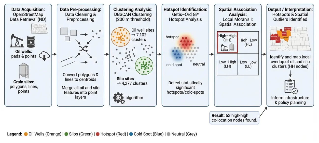
Figure 2.
Clustering of Well Point and Well Pad Centroids.
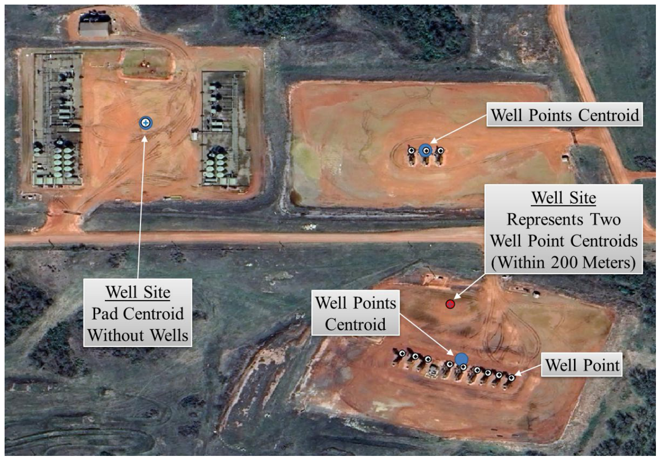
Figure 3.
Polygon, Line, and Point representation of Silos in the OSM Database.
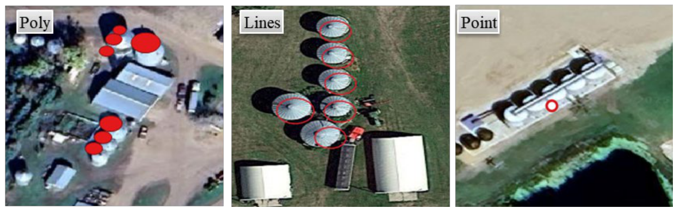
Figure 4.
Cluster centroid representing a site containing numerous silo points.
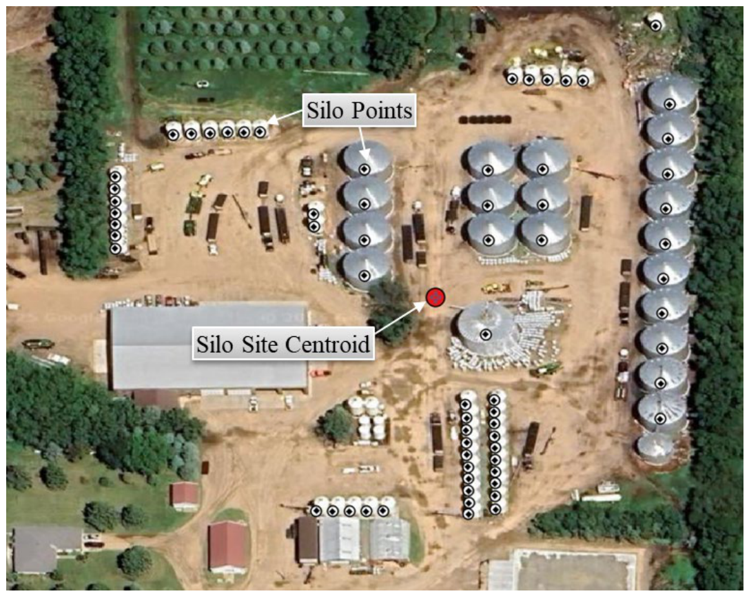
Figure 5.
HH Persistence Map.
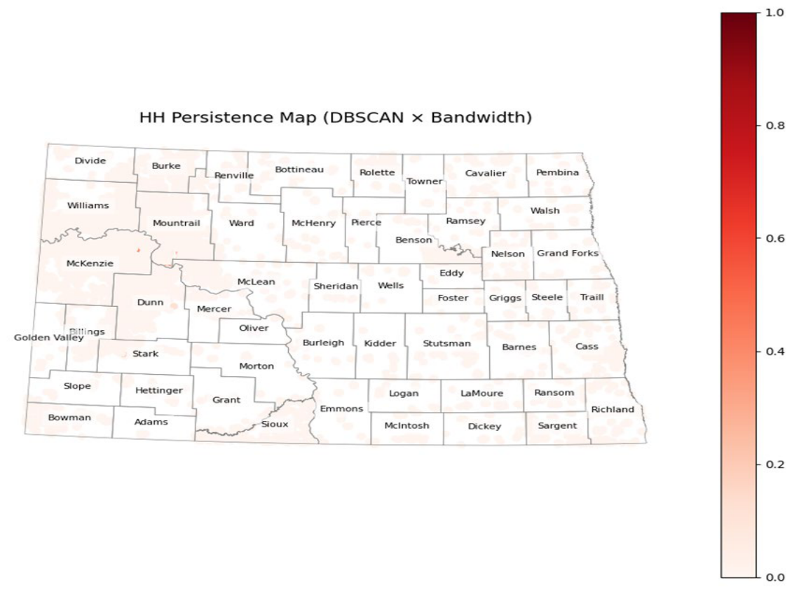
Figure 6.
Distribution of the number of neighbors for each oil well or silo site.
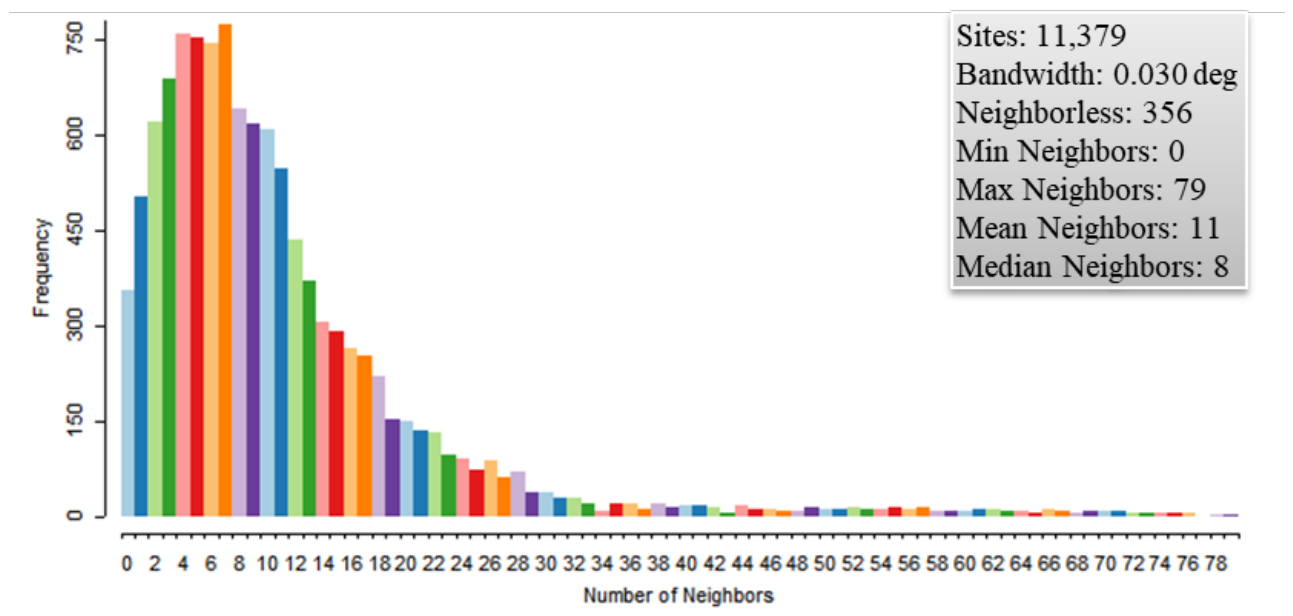
Figure 7.
Oil well counts by county and silo sites relative to oil well sites.
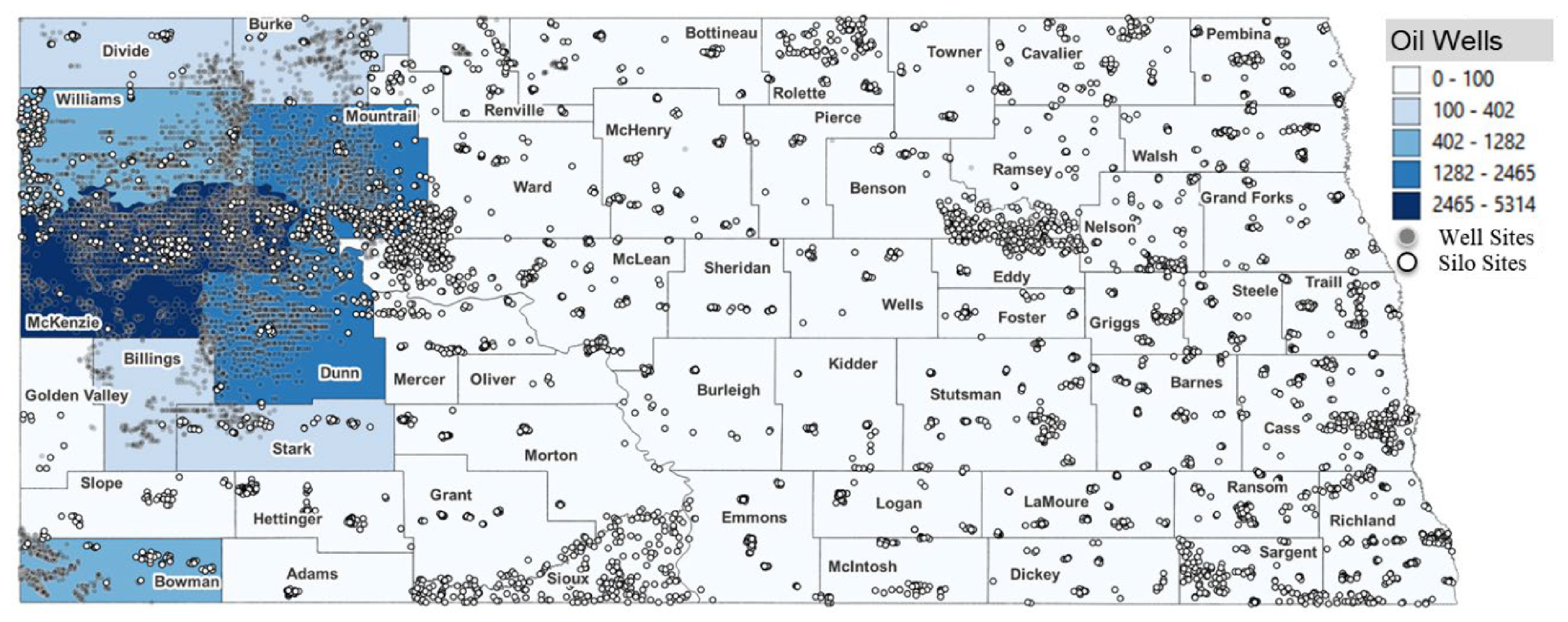
Figure 8.
Silo counts by county and silo sites relative to oil well sites.
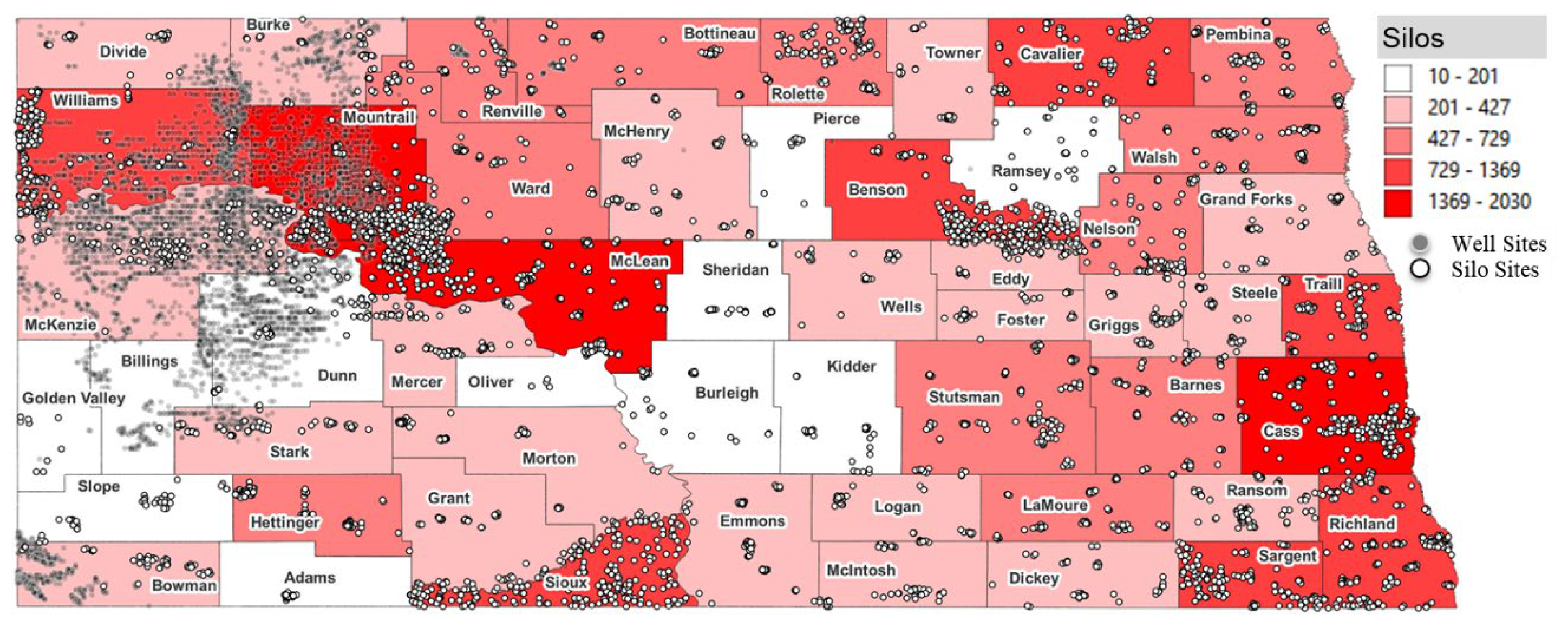
Figure 9.
Significant clusters with high and low densities of (a) oil wells and (b) silos.
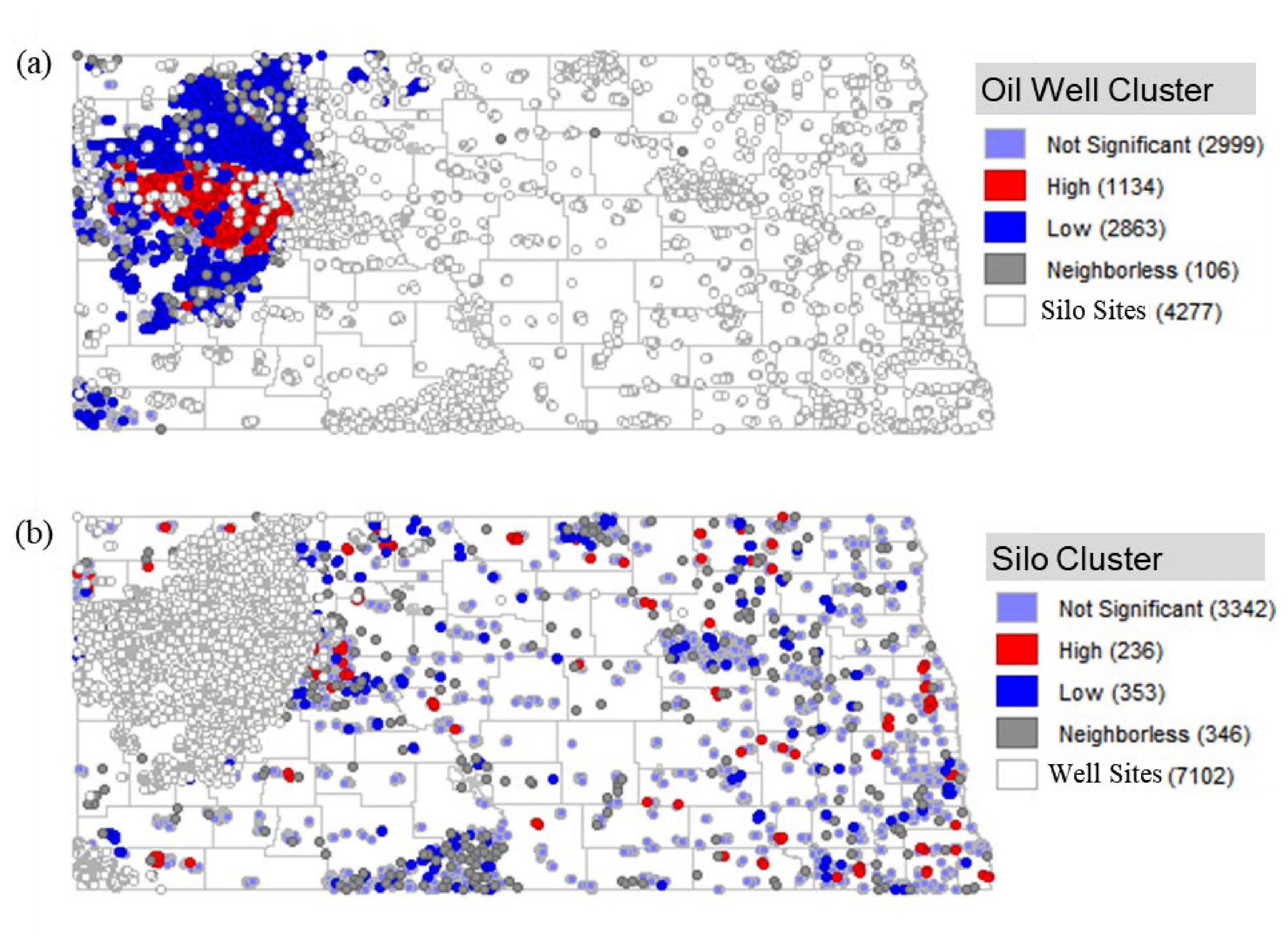
Figure 10.
Significant clustering of oil well sites.
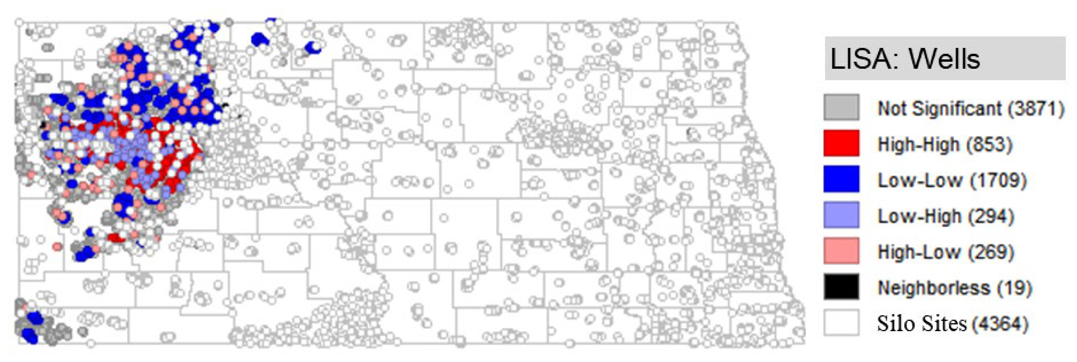
Figure 11.
Significant clustering of silo sites based on local Moran’s I analysis.
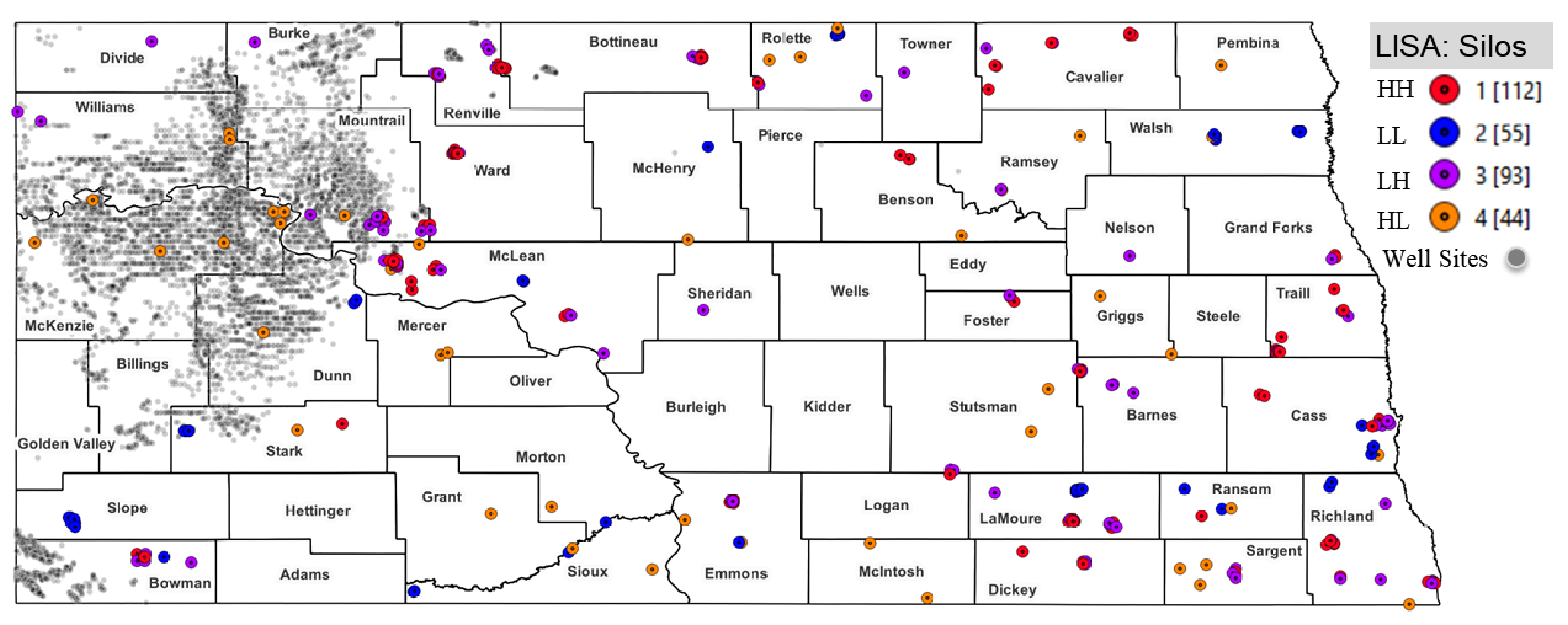
Figure 12.
Bivariate Moran’s for (a) Silos with Well neighbors and (b) a highlight of the HH cluster.
Figure 12.
Bivariate Moran’s for (a) Silos with Well neighbors and (b) a highlight of the HH cluster.
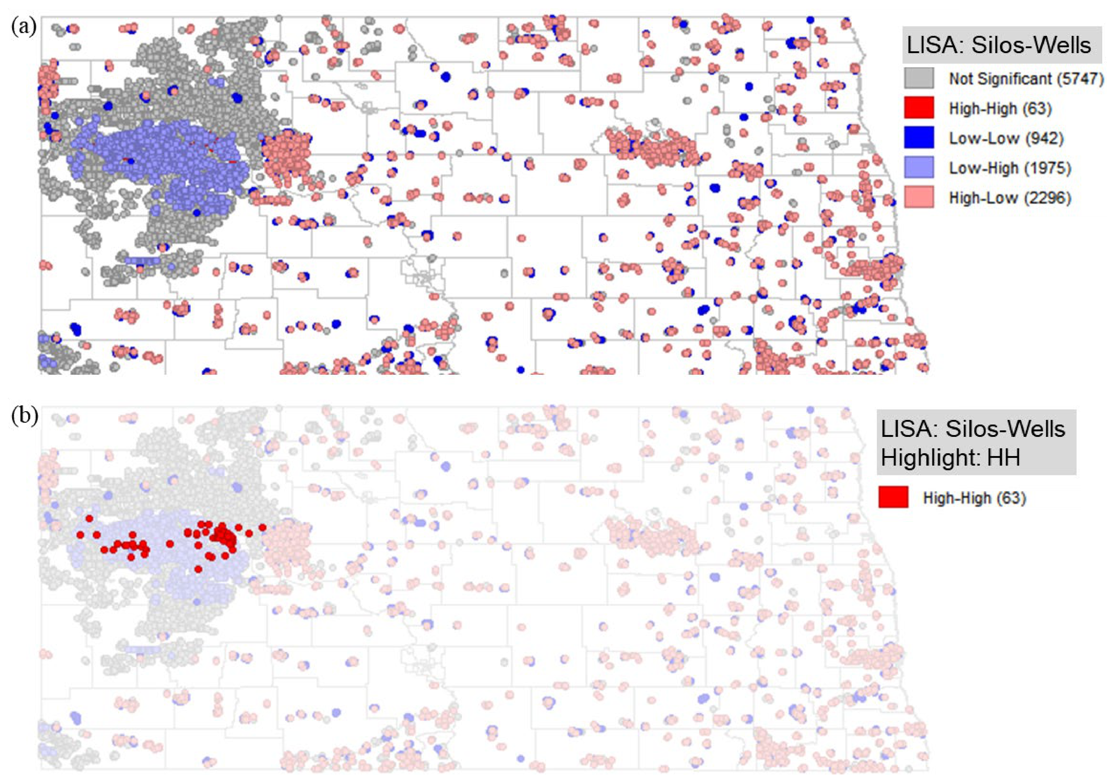
Figure 13.
Counties with HH silos-wells. Source: Satellite Imagery by Google Maps (2026).
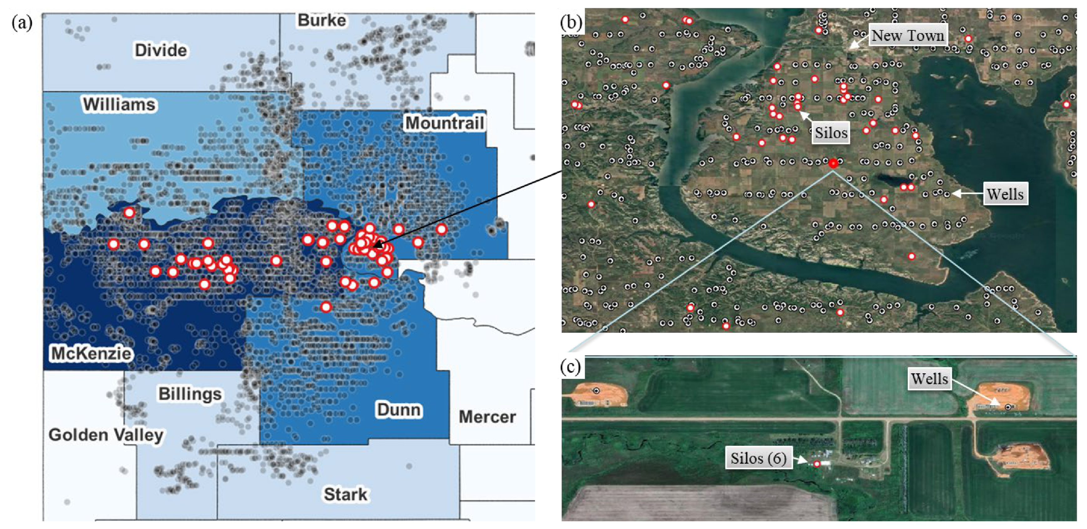
Table 1.
Results of OSM Search for Oil Wells in North Dakota.
| Returned Objects | Objects | Action |
|---|---|---|
| Oil Well Pads | 5640 | Replaced with centroid |
| Oil Substations | 4 | Deleted |
| Oil Substation Gates | 30 | Deleted |
| Oil Well Points | 7315 | Retained |
Table 2.
Results of OSM Search for Silos in North Dakota.
| Returned Objects | Objects | Action |
|---|---|---|
| Polygons | 26,131 | Replaced with centroid |
| Line | 618 | Replaced with centroid |
| Points | 627 | Replaced with centroid |
Table 4.
Bandwidth and Sensitivity Analysis. NS = not significant.
| TH | BW | MI | p-Value | HH | HL | LH | LL | NS |
|---|---|---|---|---|---|---|---|---|
| 100 | 1 | −0.247 | 0.001 | 7 | 2351 | 1107 | 2569 | 6403 |
| 100 | 2.5 | −0.282 | 0.001 | 39 | 2469 | 1782 | 1641 | 6506 |
| 100 | 5 | −0.283 | 0.001 | 72 | 2567 | 2675 | 1702 | 5421 |
| 100 | 10 | −0.279 | 0.001 | 100 | 2599 | 3423 | 1809 | 4506 |
| 100 | 20 | −0.274 | 0.001 | 113 | 2598 | 4134 | 1867 | 3725 |
| 200 | 1 | −0.210 | 0.001 | 9 | 2042 | 892 | 2204 | 6006 |
| 200 | 2.5 | −0.251 | 0.001 | 42 | 2176 | 1542 | 1233 | 6160 |
| 200 | 5 | −0.252 | 0.001 | 77 | 2319 | 2263 | 1315 | 5179 |
| 200 | 10 | −0.250 | 0.001 | 104 | 2347 | 2906 | 1439 | 4357 |
| 200 | 20 | −0.246 | 0.001 | 112 | 2377 | 3551 | 1569 | 3544 |
| 300 | 1 | −0.174 | 0.001 | 9 | 2187 | 630 | 2347 | 4819 |
| 300 | 2.5 | −0.221 | 0.001 | 29 | 2109 | 1249 | 1032 | 5573 |
| 300 | 5 | −0.223 | 0.001 | 74 | 2190 | 1967 | 1115 | 4646 |
| 300 | 10 | −0.221 | 0.001 | 94 | 2202 | 2554 | 1295 | 3847 |
| 300 | 20 | −0.218 | 0.001 | 106 | 2219 | 3076 | 1441 | 3150 |
| 400 | 1 | −0.126 | 0.001 | 8 | 1735 | 382 | 3040 | 3740 |
| 400 | 2.5 | −0.192 | 0.001 | 24 | 1646 | 892 | 1532 | 4811 |
| 400 | 5 | −0.195 | 0.001 | 56 | 1721 | 1574 | 1471 | 4083 |
| 400 | 10 | −0.194 | 0.001 | 76 | 1762 | 2146 | 1560 | 3361 |
| 400 | 20 | −0.192 | 0.001 | 86 | 1783 | 2657 | 1643 | 2736 |
| 500 | 1 | −0.067 | 0.001 | 4 | 1645 | 174 | 3049 | 3107 |
| 500 | 2.5 | −0.151 | 0.001 | 19 | 1499 | 604 | 1193 | 4664 |
| 500 | 5 | −0.158 | 0.001 | 38 | 1592 | 1177 | 1238 | 3934 |
| 500 | 10 | −0.158 | 0.001 | 70 | 1666 | 1713 | 1347 | 3183 |
| 500 | 20 | −0.156 | 0.001 | 82 | 1690 | 2195 | 1444 | 2568 |
Table 5.
Results of the FDR sensitivity analysis.
| DBSCAN (m) | Bandwidth | Moran’s I | p Value | HH Before |
HH After |
HH Retained% |
|---|---|---|---|---|---|---|
| 200 | 1 km | −0.2101 | 0.001 | 9 | 3 | 33.33 |
| 200 | 2.5 km | −0.2511 | 0.001 | 39 | 15 | 38.46 |
| 200 | 5 km | −0.2521 | 0.001 | 78 | 59 | 75.64 |
| 200 | 10 km | −0.2498 | 0.001 | 101 | 95 | 94.06 |
| 200 | 20 km | −0.2455 | 0.001 | 112 | 112 | 100.0 |
Disclaimer/Publisher’s Note: The statements, opinions and data contained in all publications are solely those of the individual author(s) and contributor(s) and not of MDPI and/or the editor(s). MDPI and/or the editor(s) disclaim responsibility for any injury to people or property resulting from any ideas, methods, instructions or products referred to in the content. |
© 2026 by the authors. Licensee MDPI, Basel, Switzerland. This article is an open access article distributed under the terms and conditions of the Creative Commons Attribution (CC BY) license (http://creativecommons.org/licenses/by/4.0/).
Copyright: This open access article is published under a Creative Commons CC BY 4.0 license, which permit the free download, distribution, and reuse, provided that the author and preprint are cited in any reuse.