
Submitted:
11 June 2026
Posted:
12 June 2026
You are already at the latest version
Abstract
Rare charm decays offer a clean arena for visible massive dark photon searches through narrow dielectron resonances. In the process D0→γA′→γe+e−, the observable signal rate is controlled simultaneously by the flavor changing charm transition, the radiative D0→γ hadronic matrix element, the visible decay probability of A′, and the experimental response of the reconstructed mass spectrum. We introduce a visible coupling formulation that combines these ingredients into a single search parameter while keeping the form factor and the A′→e+e− branching fraction as explicit external inputs. This provides a direct bridge between branching fraction sensitivity and coupling reach, without assuming a specific experimental background model. The central novelty of this approach is that it separates the particle physics information entering the signal rate from the analysis dependent ingredients that determine the observable mass spectrum. We apply this construction to the D0→γe+e− spectrum, including effective exposure, reconstruction efficiency, mass resolution, and the treatment of the ρ/ω and ϕ regions. The ρ/ω and ϕ dominated intervals are kept outside the coupling definition and left to experiment specific resonance treatment. This formulation gives a practical and reusable basis for comparing visible massive dark photon sensitivity across current and future charm data sets.
Keywords:
massive dark photon
; rare charm decay
; benchmark
; sensitivity
1. Introduction
A massive dark photon provides a well-motivated low-energy window onto hidden vector interactions. If the new boson has a nonzero mass, it can be produced on shell and searched for as a localized structure in a visible invariant-mass spectrum. In the minimal kinetic-mixing picture, constraints are commonly displayed in the - plane, and extensive fixed-target, , and hadron-collider programs have explored both visible and invisible decays [1,2,3,4,5,6]. This organization is most transparent when production and decay are governed by flavor-universal kinetic mixing[7,8]. It becomes less direct when the production vertex is flavor changing, because a visible final-state limit then constrains not only a microscopic coupling but also short-distance flavor dynamics, non-perturbative hadronic input, and the visible decay probability of the massive [9,10].
Rare charm decays are a natural setting for such a study. Standard Model flavor changing neutral current amplitudes in the up-quark sector are strongly suppressed, while exclusive charm modes are strongly affected by long distance hadronic effects and vector-meson resonances [11,12,13,14,15,16,17]. Consequently, inclusive rates alone are often difficult to interpret, whereas narrow structures and differential null tests can provide cleaner sensitivity to short-distance contributions [18,19,20,21,22,23]. Existing measurements and searches in radiative and dileptonic charm channels, including , , , , and , demonstrate the feasibility of such final states while emphasizing the need for controlled continuum and , -region treatments [24,25,26,27,28,29]. The recent BESIII search for a massless dark photon in decays is therefore closely related, but the massive visible case considered here is experimentally and interpretively distinct because the is reconstructed through [30].
The study focuses on with . The signal topology is illustrated in Figure 1. The channel combines a two-body radiative production process with a narrow dielectron resonance search, but its rate cannot be mapped to a single microscopic parameter without additional assumptions. It depends simultaneously on the short-distance transition, the hadronic matrix element at , and the branching fraction for . The experimentally useful mass range is further shaped by photon and electron reconstruction, bremsstrahlung recovery, conversion backgrounds, endpoint phase-space suppression, and resonance vetoes or templates near the and bands. A direct bound on would therefore mix detector sensitivity with hadronic and model-dependent inputs.
To keep these ingredients separate, we parameterize the flavor-changing transition by an effective dipole operator and retain the hadronic transition as an explicit factor . We then combine this factor and the visible branching fraction with the effective dipole strength into a visible coupling . In this normalization, is proportional to multiplied by the cubic two-body phase-space factor, so an experimental branching-fraction sensitivity can be converted into a reach without fixing a particular ultraviolet completion, form-factor model, or decay scenario. Detector-level inputs from BESIII-like, Belle II-like, LHCb-like, or future samples enter through the effective exposure, efficiency, mass resolution, background level, and resonance treatment [31,32,33,34]. The resulting framework is therefore a portable normalization for searches for a massive visible in , with later translations to or left to model-specific input.
2. Effective Description and Visible Normalization
In this benchmark, the signal topology can be organized into two main ingredients that are useful to treat separately at the outset. The first is the short-distance flavour changing transition , which is described by an effective operator at the charm scale. The second is the long-distance hadronic transition in which the meson emits the photon. Keeping these two ingredients separate makes the normalization transparent and allows the hadronic input to be updated independently.
At the lowest non-trivial order, the short distance flavor changing transition is represented by the dipole interaction,
where is the field strength tensor of the vector state , , and C and are dimensionless Wilson coefficients. The scale represents the heavy mass scale that suppresses the dimension-five operator.
In this benchmark, the term dark photon is used in a broad phenomenological sense: it denotes a massive visible vector state that can decay into . The flavor changing production vertex is not assumed to arise from minimal kinetic mixing alone, but is parameterized directly by the effective dipole operator in Equation (1). Consequently, translating the effective normalization introduced below into the conventional kinetic mixing parameter requires additional theoretical input, as discussed in Section 4.
For an unpolarized benchmark rate, and under the common form factor normalization introduced below, the two dipole structures enter through the quadratic combination
This definition should be understood as a convenient low energy coupling strength. It does not assume a specific ultraviolet model, nor does it fix possible CP phases that would require a more differential analysis.
The remaining part of the amplitude is the non-perturbative hadronic matrix element for the transition. Rather than assigning a model-dependent numerical value to this matrix element, we absorb it into a dimensionless transition factor , evaluated at . To make this convention explicit, we fix the normalization of through the polarization summed amplitude,
With this definition, Equation (3) should be regarded as a normalization convention rather than as an independent dynamical prediction. The factor displays the momentum dependence generated by the radiative dipole structure, while the unknown strong-interaction normalization is kept in . With this convention, lattice QCD calculations, light-cone sum rule estimates, vector-meson dominance inputs, or data driven normalizations can be incorporated simply by replacing , without changing the kinematic conversion used later.
The experimentally reconstructed final state is , rather than the intermediate state alone. The observable rate must therefore include the probability for to decay into an electron and positron pair. We combine the coupling associated with the short distance transition, the hadronic normalization, and the visible branching fraction into a coupling used at the search level,
The quantity has the same mass dimension as , namely . All projected rates in the following analysis are expressed in terms of . If a particular model later specifies both and , the same results can be translated back to , and then to the microscopic parameters of that model.
3. Signal Branching Fraction from Two-Body Kinematics
After the visible normalization has been specified, the signal rate can be obtained from the two body decay . In the rest frame of the meson, and treating the photon as massless, the common momentum of the two final state particles is
This expression is purely kinematic. It shows that the available momentum vanishes when the mass of approaches the mass.
Throughout this benchmark we consider the visible massive- range
The lower bound follows from the requirement that the intermediate state can decay into an pair, while the upper bound is set by the two-body kinematics of . In practice, the experimentally useful region is further restricted by reconstruction thresholds, conversion backgrounds, resonance regions, and endpoint phase-space loss, as discussed below.
The partial width is obtained by multiplying the squared amplitude by the two body phase space. Since the parent meson has spin zero, no average over initial spin states is required. After summing over the final state polarizations, one obtains
Substituting the amplitude normalization introduced in Equation (3) and the momentum in Equation (5) gives
Here the transition factor is evaluated at . The cubic dependence has a clear kinematic origin: one power arises from the two body phase space, while the remaining two powers are supplied by the radiative dipole structure of the amplitude.
The experimentally visible final state also requires the decay of into an electron pair. Therefore, the partial width must be multiplied by and by the visible branching fraction. Using the definition of , the visible signal branching fraction becomes
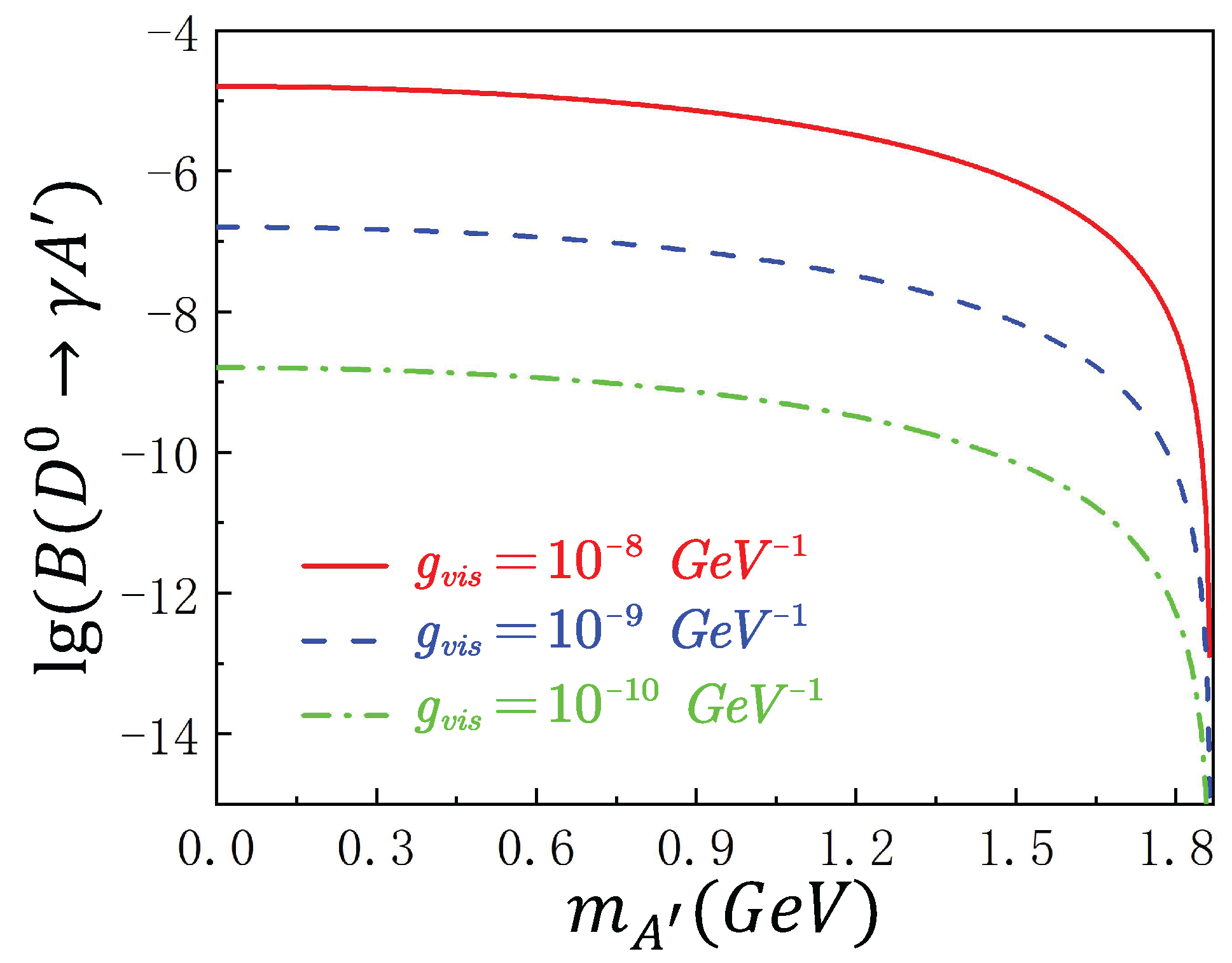
For this benchmark, Equation (9) is the main conversion between the coupling used at the search level and the visible branching fraction. It shows that the rate is proportional to and that the rate is suppressed when the available two-body momentum becomes small near the endpoint. The corresponding benchmark branching fraction curves, which visualize the scaling and the endpoint suppression implied by Equation (9), are shown in Appendix A.
The same branching fraction fixes the area of the peak in the reconstructed dielectron mass spectrum. If the intrinsic width of is much smaller than the detector mass resolution, the observed signal is controlled by the detector response. For a normalized resolution function G,
where the normalization of G ensures that the integral of the peak is . If the intrinsic width is not negligible compared with the mass resolution, the physical line shape should first be described by a normalized Breit Wigner function and then smeared with the detector response,
The narrow peak expression in Equation (10) is used as a transparent benchmark for a weakly coupled visible state. It fixes the signal yield and the local peak shape, but it does not replace the background model of a real analysis. In an experimental study, the smooth continuum, sidebands, reconstruction efficiency, and the , resonance regions should be treated with experiment-specific templates or vetoes.
4. Coupling Reach and Interpretation
The preceding section gives a direct relation between the visible branching fraction and the coupling used at the search level. This relation can be inverted to express the coupling reach in terms of a detector level sensitivity to the visible branching fraction. Denoting this sensitivity by , and solving Equation (9) for , one obtains
This expression is the conversion used to draw the coupling reach curves. The square root dependence reflects the fact that rates are proportional to squared amplitudes. As a result, an improvement of the branching fraction sensitivity by a factor of ten improves the coupling reach by a factor of . The last factor shows the loss of reach near the kinematic endpoint, where the two body phase space becomes small.
Figure 2 shows the reach in obtained from representative values of . The curves depend only on the visible branching fraction sensitivity and on the kinematic factor in Equation (12). The rise at large is therefore not a consequence of an assumed background model, but follows from the closing of the available phase space.
Table 1 gives representative numerical values of the converted coupling reach. These values are consistent with Equation (12), using the mass, the lifetime, and ℏ in units matched to GeV. The table is intended as a benchmark for rescaling rather than as a substitute for an experiment specific limit.
Expressing the reach in terms of keeps the detector-level sensitivity separated from the hadronic normalization and from the visible decay probability of the intermediate state. The quantity should therefore not be read as a microscopic coupling by itself. It already contains the hadronic transition factor and the visible branching fraction of . Once a specific model or a data driven input provides these quantities, the corresponding effective coupling is obtained from
Here the transition factor is evaluated at . This equation separates the experimental result from the external physics inputs. The experimental analysis constrains , while the conversion to requires information on the hadronic normalization and on the decay probability of into the electron pair. In this sense, is the most model-independent quantity to quote, whereas should be reported only after specifying and . Different choices of these two inputs therefore rescale the same reach multiplicatively, without changing the detector-level conversion in Equation (12).
Figure 3 visualizes the reinterpretation step encoded in Equation (13). For a fixed detector level reach on the search level coupling , the inferred constraint on the underlying effective flavor changing coupling depends on two external inputs: the hadronic transition normalization and the visible decay probability . The color scale therefore represents the multiplicative factor that converts a quoted limit into an input-dependent limit. Smaller values of either input weaken the inferred constraint on , even when the experimental sensitivity to is unchanged. Thus, Figure 3 should not be interpreted as imposing a particular form factor model or dark sector decay scenario. Instead, it provides a rescaling map that allows future theoretical or phenomenological inputs to be applied to the same experimental search level result. This makes explicit the central separation of the present framework: detector level sensitivity is encoded in , whereas the translation to is left to external theoretical input.
With this separation made explicit, the representation provides a useful way to position the present framework relative to other research perspectives. Unlike the conventional versus plane used in ordinary dark photon searches, the present benchmark is organized around a charm transition with changing flavor and a visible intermediate state. Table 2 summarizes this distinction and compares the role of the framework with related approaches.
This comparison clarifies the scope of the benchmark. Ordinary dark photon searches provide important external context, but they do not directly constrain the amplitude without additional assumptions. Rare charm studies are closer in motivation, although they are often sensitive to long distance hadronic effects. Standard Model studies of the visible decay spectrum are essential for modeling the continuum, sidebands, and resonance regions. The formulation is therefore best understood as a reusable normalization that connects visible sensitivity at the detector level to a charm transition with changing flavor, while the translation to , microscopic couplings, or the kinetic mixing parameter requires external hadronic and decay inputs.
5. Yield, Sensitivity, and Resonance Treatment
The visible branching fraction obtained above can be converted into an expected event yield once the effective exposure is specified. We define the effective exposure as the number of reconstructed candidates multiplied by the total signal efficiency. With this definition,
where includes the relevant reconstruction and selection effects. If both and samples are used, should denote the total number of neutral charm mesons included in the analysis. This relation gives the basic scaling of the signal yield with exposure and branching fraction.
For a search at a fixed value of , the signal is counted in a mass window W centered on the tested mass. The expected signal and background yields in this window can be written as
Here denotes the fraction of the signal line shape contained in the chosen window. The function describes this mass-dependent background efficiency, and denotes the corresponding differential background branching fraction before detector effects.
For each tested value of , the window yields S and B are converted into a local sensitivity according to an experiment-specific statistical criterion. Since this work is intended as a normalization benchmark, we do not prescribe a unique discovery or exclusion test. Instead, we define as the minimum signal yield required by the adopted counting or likelihood procedure. This quantity may depend on the expected background, systematic uncertainties, the mass window definition, and, in a mass scan, the treatment of the look-elsewhere effect.
The same counting setup also determines the branching fraction sensitivity that enters Equation (12). Solving Equation (15) for the signal branching fraction and replacing S by gives
In the background-free 90% C.L. limit, one may use . In the background-dominated case, is obtained by solving the chosen local significance or exclusion condition using the statistical model specified above. The resulting is therefore a sensitivity at the tested mass point. In a mass scan, this local sensitivity should be distinguished from a global exclusion or discovery criterion, since scanning many tested masses increases the probability of finding a background fluctuation somewhere in the spectrum.
A schematic mass spectrum can then be written as a sum of normalized templates,
where describes the smooth continuum, denotes the vector meson templates for , , and G denotes the detector resolution template for the signal. The coefficients , , and are the corresponding event yields. The structure of Equation (17) is illustrated schematically in Figure 4.
Figure 4 provides a visual representation of the template decomposition in Equation (17). The blue dashed curve represents the smooth continuum component , while the red dashed structures indicate the vector-meson contributions associated with the and regions. The green narrow peaks illustrate potential signal contributions at possible mass values. The shaded vertical bands emphasize the resonance-dominated mass intervals, where the interpretation of a narrow visible signal is expected to be most analysis dependent.
Equation (17) is intended only as a schematic description of the mass spectrum. It should not be read as a unique Standard Model background prediction. In a real analysis, the continuum shape, sidebands, reconstruction efficiency, and resonance regions should be treated with experiment specific templates or vetoes. If interference among resonant and continuum amplitudes is relevant, the template sum should be replaced by an amplitude level model.
The and regions are therefore the main limitations for a visible-spectrum interpretation. In the benchmark presentation, the intervals near 0.72 - 0.82 GeV and 0.99 - 1.04 GeV can be treated either as veto regions or as regions that require dedicated vector-meson templates. This treatment preserves the usefulness of the signal normalization while avoiding an overinterpretation of the schematic spectrum in regions dominated by known hadronic structures.
Taken together, the yield, significance, and spectrum relations provide a practical way to reinterpret a detector-level search in terms of the visible coupling defined above. Their cleanest use is in regions where the intermediate state is narrow compared with the experimental mass resolution and where the visible decay can be treated as prompt, so that the acceptance effects are contained in . Near the and bands, the same normalization can still be used, but the spectral interpretation should be tied to experiment-specific vetoes or resonance templates. With these qualifications, the framework provides a reusable conversion between visible branching fraction sensitivity, reach, and exposure scaling, while translations to or to the ordinary kinetic-mixing parameter require additional hadronic or model input. Representative detector-level inputs for BESIII-like, Belle II-like, and LHCb-like massive searches are summarized in Appendix B. These inputs are used only for rescaling purposes and are not treated as existing limits on the specific decay chain.
6. Conclusions
Rare charm searches with visible narrow structures are difficult to interpret in a single microscopic parameter because the observed rate depends simultaneously on the short-distance transition, the non-perturbative matrix element, and the visible decay probability of the intermediate state. In this work, we have organized these ingredients into a visible coupling benchmark for the decay chain . The definition of keeps the detector level sensitivity separated from the hadronic and visible decay inputs, so that experimental branching fraction sensitivities can be compared without committing to a specific ultraviolet completion.
Within this normalization, the visible branching fraction is controlled by and by the cubic two-body phase space factor. The inverse relation then converts a representative sensitivity into a reach on , with the expected degradation near the kinematic endpoint. The same framework also connects the branching fraction reach to event yields through the effective exposure , making it straightforward to rescale the benchmark to different reconstructed charm samples, efficiencies, and mass resolutions.
The resulting formulation is intended as a rescaling tool rather than as a universal bound on the kinetic mixing parameter. Once experiment-specific efficiencies, background templates, resonance vetoes, and mass scan procedures are specified, the formulae can be used to compare BESIII-like, Belle II-like, LHCb-like, or future charm samples in a common visible coupling language. A further translation from to or to microscopic dark sector parameters requires additional input on and .
Author Contributions
Conceptualization, methodology, data analysis and original draft preparation, Xin Zhong; Validation, Jianshan Wang; writing review and editing, Jianshan Wang and Shuping Shan. All authors have read and agreed to the published version of the manuscript.
Funding
This study was supported by the Fujian Province Young and Middle-aged Scientists Fund (grants JAT241139), the Fujian Province Natural Science Fund General Project (grant 2025J011710), and the Longyan University Doctoral Research Startup Projects 2025 (grants LB2025003).
Data Availability Statement
The raw data supporting the conclusions of this article will be made available by the authors on request.
Conflicts of Interest
The authors declare no conflicts of interest.
Appendix A
Figure A1 illustrates the benchmark branching fraction implied by the visible coupling normalization. For fixed , the signal branching fraction is controlled entirely by the quadratic coupling dependence and by the cubic two-body phase space factor. The three curves are separated by two orders of magnitude in for each one order of magnitude change in , reflecting the scaling . The common downward turn as approaches the mass is the endpoint suppression from . This figure therefore shows the clean kinematic part of the benchmark normalization, while the translation to requires the external inputs and .
Figure A1.
Benchmark signal branching fraction for as a function of the dark photon mass .
Appendix B
Table A1 summarizes representative detector level benchmark inputs for BESIII-like, Belle II-like, and LHCb-like massive visible- searches.

| Scenario | Massive relevance | Benchmark input | Useful region | Main experimental issue |
|---|---|---|---|---|
| BESIII-like | Tagged environment; suitable for a prompt narrow peak recoiling against a photon. | - ; - 8 MeV | Low and intermediate masses, away from vector meson regions. | Statistics, photon reconstruction, conversion background, and , treatment. |
| Belle II-like | High luminosity environment with large charm samples; useful for a broad scan. | - ; - 10 MeV | Broad range below the kinematic endpoint. | Continuum background, photon efficiency, bremsstrahlung recovery, and mass dependent efficiency. |
| LHCb-like | Large prompt charm yield and rare charm experience with final states; useful in selected prompt windows. | - ; - 15 MeV | Selected prompt windows outside resonance dominated regions. | Selection efficiency, low mass electron reconstruction, nonuniform acceptance, and template control. |
For a given scenario in Table A1, the quoted and do not by themselves determine . The latter also depends on the mass window efficiency , the background level in the tested window, the treatment of resonance regions, and the adopted statistical criterion. In a simple background free estimate, Equation (16) reduces to .
These benchmark scenarios are designed for a massive visible dark photon, reconstructed as a narrow structure in the spectrum. They should not be interpreted as published limits on . Instead, they provide representative detector-level inputs for applying the conversion in Equation (12). Since the reach scales with the phase space factor , the sensitivity deteriorates as approaches the endpoint. In addition, the regions around the and resonances require either vetoes or dedicated vector-meson templates.
References
- Galison, P.; Manohar, A. Two Z’s or not two Z’s? Phys. Lett. B 1984, 136, 279–283. [Google Scholar] [CrossRef]
- Holdom, B. Two U(1)’s and ϵ Charge Shifts. Phys. Lett. B 1986, 166, 196–198. [Google Scholar] [CrossRef]
- Pospelov, M.; Ritz, A.; Voloshin, M.B. Secluded WIMP Dark Matter. Phys. Lett. B 2008, 662, 53–61. [Google Scholar] [CrossRef]
- Arkani-Hamed, N.; Finkbeiner, D.P.; Slatyer, T.R.; Weiner, N. A Theory of Dark Matter. Phys. Rev. D 2009, 79, 015014. [Google Scholar] [CrossRef]
- Essig, R.; Schuster, P.; Toro, N. Probing Dark Forces and Light Hidden Sectors at Low-Energy e+e- Colliders. Phys. Rev. D 2009, 80, 015003. [Google Scholar] [CrossRef]
- Bjorken, J.D.; Essig, R.; Schuster, P.; Toro, N. New Fixed-Target Experiments to Search for Dark Gauge Forces. Phys. Rev. D 2009, 80, 075018. [Google Scholar] [CrossRef]
- Raggi, M.; Kozhuharov, V. Results and perspectives in dark photon physics. Riv. Nuovo Cim. 2015, 38, 449–505. [Google Scholar]
- Lanfranchi, G.; Pospelov, M.; Schuster, P. The Search for Feebly Interacting Particles. Annu. Rev. Nucl. Part. Sci. 2021, 71, 279–313. [Google Scholar] [CrossRef]
- Ilten, P.; Soreq, Y.; Thaler, J.; Williams, M.; Xue, W. Dark Photons from Charm Mesons at LHCb. Phys. Rev. D 2015, 92, 115017. [Google Scholar] [CrossRef]
- Ilten, P.; Thaler, J.; Williams, M.; Xue, W. Proposed Inclusive Dark Photon Search at LHCb. Phys. Rev. Lett. 2016, 116, 251803. [Google Scholar] [CrossRef]
- Glashow, S.L.; Iliopoulos, J.; Maiani, L. Weak Interactions with Lepton-Hadron Symmetry. Phys. Rev. D 1970, 2, 1285–1292. [Google Scholar] [CrossRef]
- Burdman, G.; Golowich, E.; Hewett, J.L.; Pakvasa, S. Rare Charm Decays in the Standard Model and Beyond. Phys. Rev. D 2002, 66, 014009. [Google Scholar] [CrossRef]
- Fajfer, S.; Prelovsek, S.; Singer, P. Resonant and Nonresonant Contributions to the Weak D→Vℓ+ℓ- Decays. Phys. Rev. D 1998, 58, 094038. [Google Scholar] [CrossRef]
- Fajfer, S.; Prelovsek, S.; Singer, P. Rare Charm Meson Decays D→Pℓ+ℓ- and c→uℓ+ℓ- in the Standard Model and MSSM. Phys. Rev. D 2001, 64, 114009. [Google Scholar] [CrossRef]
- Fajfer, S.; Kosnik, N.; Prelovsek, S. Updated Constraints on New Physics in Rare Charm Decays. Phys. Rev. D 2007, 76, 074010. [Google Scholar] [CrossRef]
- Paul, A.; Bigi, I.I.; Recksiegel, S. On D→Xuℓ+ℓ- within the Standard Model and Frameworks Like the Littlest Higgs Model with T Parity. Phys. Rev. D 2011, 83, 114006. [Google Scholar] [CrossRef]
- Cappiello, L.; Cata, O.; D’Ambrosio, G. Standard Model Prediction and New Physics Tests for D0→h+h-ℓ+ℓ- (h=π,K; ℓ=e,μ). JHEP 2013, 04, 135. [Google Scholar] [CrossRef]
- de Boer, S.; Hiller, G. Flavor and New Physics Opportunities with Rare Charm Decays into Leptons. Phys. Rev. D 2016, 93, 074001. [Google Scholar] [CrossRef]
- de Boer, S.; Hiller, G. Rare Radiative Charm Decays within the Standard Model and Beyond. JHEP 2017, 08, 091. [Google Scholar] [CrossRef]
- de Boer, S.; Hiller, G. Null Tests from Angular Distributions in D→P1P2ℓ+ℓ-, ℓ=e,μ Decays on and off Peak. Phys. Rev. D 2018, 98, 035041. [Google Scholar] [CrossRef]
- Gisbert, H.; Golz, M.; Mitzel, D.S. Theoretical and Experimental Status of Rare Charm Decays. Mod. Phys. Lett. A 2021, 36, 2130002. [Google Scholar] [CrossRef]
- Bause, R.; Gisbert, H.; Golz, M.; Hiller, G. Exploiting CP Asymmetries in Rare Charm Decays. Phys. Rev. D 2020, 101, 115006. [Google Scholar] [CrossRef]
- Bause, R.; Golz, M.; Hiller, G.; Tayduganov, A. The New Physics Reach of Null Tests with D→πℓ+ℓ- and Ds→Kℓ+ℓ- Decays. Eur. Phys. J. C 2020, 80, 65. [Google Scholar] [CrossRef]
- Tajima, O.; Abe, K.; Abe, K.; Adachi, I.; Aihara, H.; Anipko, D.; Aulchenko, V.; Aushev, T.; Bakich, A.M.; Barberio, E.; et al. Observation of Radiative Decay D0→ϕγ. Phys. Rev. Lett. 2004, 92, 101803. [Google Scholar] [CrossRef] [PubMed]
- Aubert, B.; Bona, M.; Boutigny, D.; Karyotakis, Y.; Lees, J.P.; Poireau, V.; Tisserand, V.; Zghiche, A.; Grauges, E.; Palano, A.; et al. Measurement of the Branching Fractions of the Radiative Charm Decays D0→K*0γ and D0→ϕγ. Phys. Rev. D 2008, 78, 071101. [Google Scholar] [CrossRef]
- Ablikim, M.; Achasov, M.N.; Ai, X.C.; Albayrak, O.; Albrecht, M.; Ambrose, D.J.; Amoroso, A.; An, F.F.; An, Q.; Bai, J.Z.; et al. Search for D0→γγ and Improved Measurement of the Branching Fraction for D0→π0π0. Phys. Rev. D 2015, 91, 112015. [Google Scholar] [CrossRef]
- Nanut, T.; Adachi, I.; Aihara, H.; Al Said, S.; Asner, D.M.; Aushev, T.; Ayad, R.; Babu, V.; Badalov, A.M.; Badhrees, I.; et al. Observation of D0→ρ0γ and Search for CP Violation in Radiative Charm Decays. Phys. Rev. Lett. 2017, 118, 051801. [Google Scholar] [CrossRef] [PubMed]
- Aaij, R.; Adeva, B.; Adinolfi, M.; Ajaltouni, Z.; Albrecht, J.; Alessio, F.; Alexander, M.; Ali, S.; Alkhazov, G.; Alvarez Cartelle, P.; et al. Observation of D0 Meson Decays to π+π-μ+μ- and K+K-μ+μ- Final States. Phys. Rev. Lett. 2017, 119, 181805. [Google Scholar] [CrossRef] [PubMed]
- Lees, J.P.; Poireau, V.; Tisserand, V.; Garra Tico, J.; Grauges, E.; Palano, A.; Eigen, G.; Stugu, B.; Brown, D.N.; Kolomensky, Y.G.; et al. Observation of the Decay D0→K-π+e+e-. Phys. Rev. Lett. 2019, 122, 081802. [Google Scholar] [CrossRef]
- Ablikim, M.; Achasov, M.N.; Adlarson, P.; Afedulidis, K.; Ai, X.C.; Aliberti, R.; Amoroso, A.; An, Q.; Bai, X.H.; Bai, Y.; et al. Search for a Massless Dark Photon in c→uγ′ Decays. Phys. Rev. D 2025, 111, L011103. [Google Scholar] [CrossRef]
- Ablikim, M.; An, Z.H.; Bai, J.Z.; Berger, N.; Bian, J.M.; Cai, X.; Cao, G.F.; Cao, X.X.; Chang, J.F.; Chen, C.; et al. Design and Construction of the BESIII Detector. Nucl. Instrum. Methods Phys. Res. A 2010, 614, 345–399. [Google Scholar] [CrossRef]
- Alves, A.A.; Andrade Filho, L.M.; Barbosa, A.F.; Bediaga, I.; Cernicchiaro, G.; Guerrer, G.; Lima, H.P.; Machado, A.A.; Magnin, J.; Marujo, F.; et al. The LHCb Detector at the LHC. JINST 2008, 3, S08005. [Google Scholar]
- Cowan, G.; Cranmer, K.; Gross, E.; Vitells, O. Asymptotic Formulae for Likelihood-Based Tests of New Physics. Eur. Phys. J. C 2011, 71, 1554. [Google Scholar] [CrossRef]
- Navas, S.; Amsler, C.; Gutsche, T.; Hanhart, C.; Hernández-Rey, J.J.; Lourenço, C.; Masoni, A.; Mikhasenko, M.; Mitchell, R.E.; Patrignani, C.; et al. Review of Particle Physics. Phys. Rev. D 2024, 110, 030001. [Google Scholar] [CrossRef]
- Adachi, I.; Browder, T.E.; Križan, P.; Tanaka, S.; Ushiroda, Y. Detectors for Extreme Luminosity: Belle II. Nucl. Instrum. Methods Phys. Res. A 2018, 907, 46–59. [Google Scholar] [CrossRef]
Figure 1.
Feynman diagram for the signal process , followed by the visible decay . The shaded vertex denotes the effective flavor changing transition.
Figure 1.
Feynman diagram for the signal process , followed by the visible decay . The shaded vertex denotes the effective flavor changing transition.
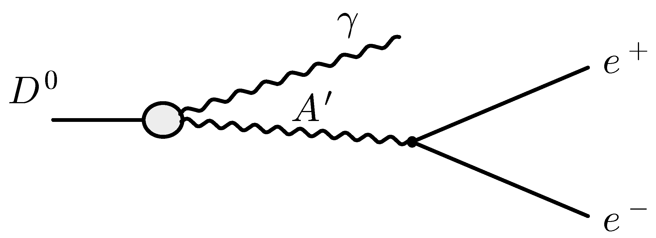
Figure 2.
Coupling reach obtained by converting detector-level branching-fraction sensitivities into . The curves correspond to , , and .
Figure 2.
Coupling reach obtained by converting detector-level branching-fraction sensitivities into . The curves correspond to , , and .
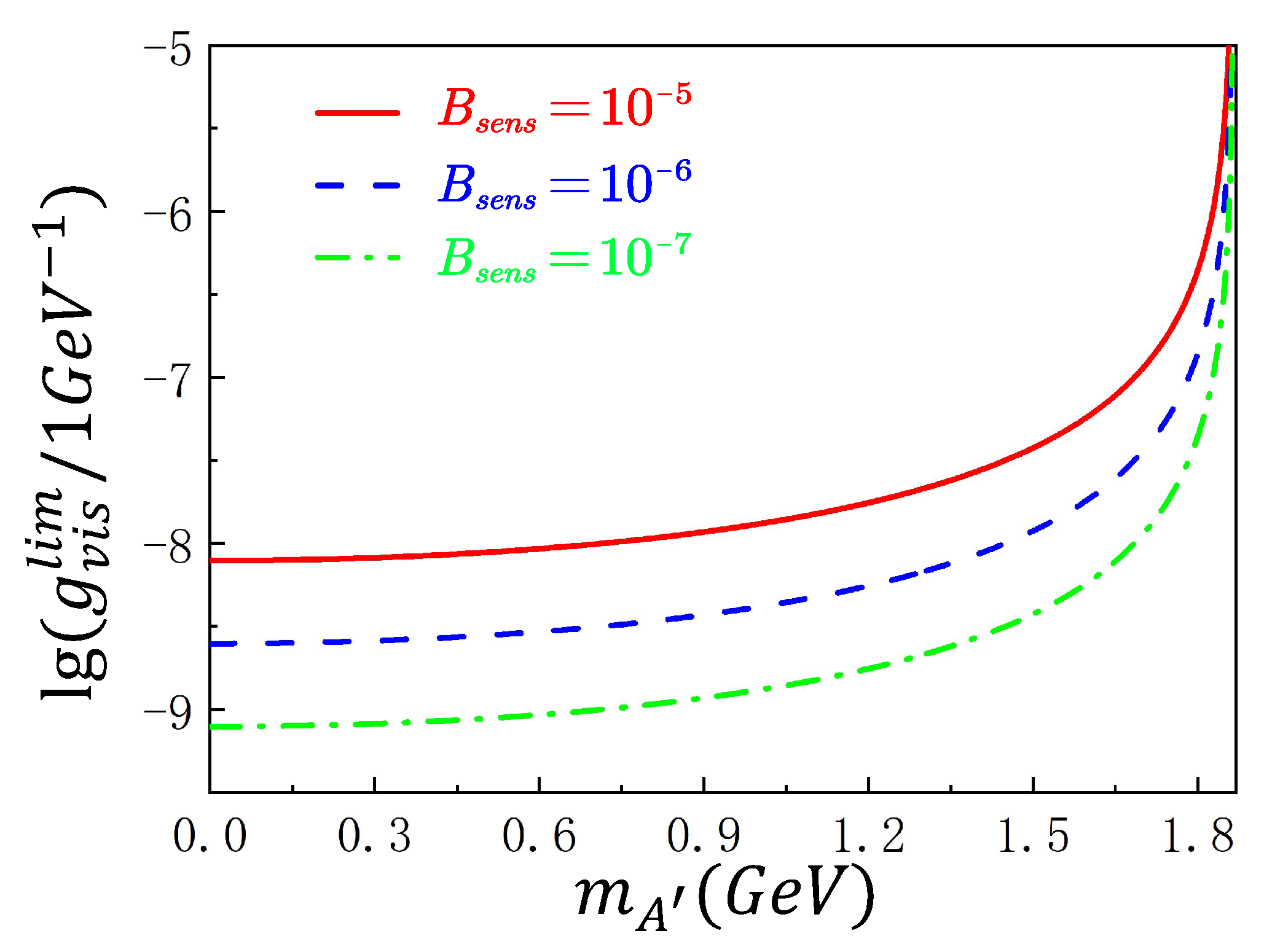
Figure 3.
Rescaling from the visible search level coupling to the effective flavor changing coupling . The color scale shows as a function of the hadronic transition normalization and the visible branching fraction .
Figure 3.
Rescaling from the visible search level coupling to the effective flavor changing coupling . The color scale shows as a function of the hadronic transition normalization and the visible branching fraction .
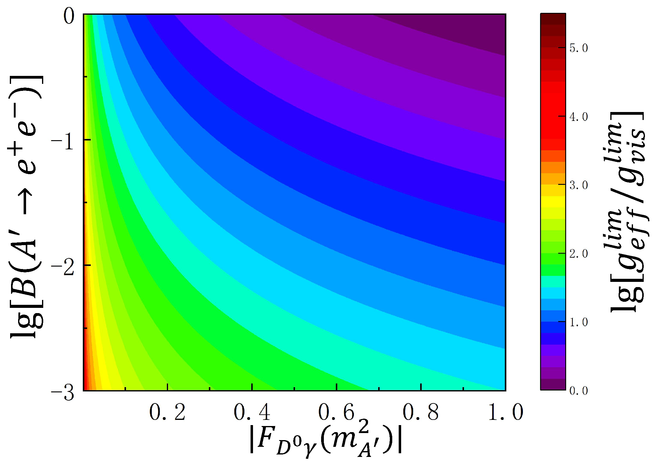
Figure 4.
Schematic normalized dielectron invariant-mass spectrum for the visible search in .
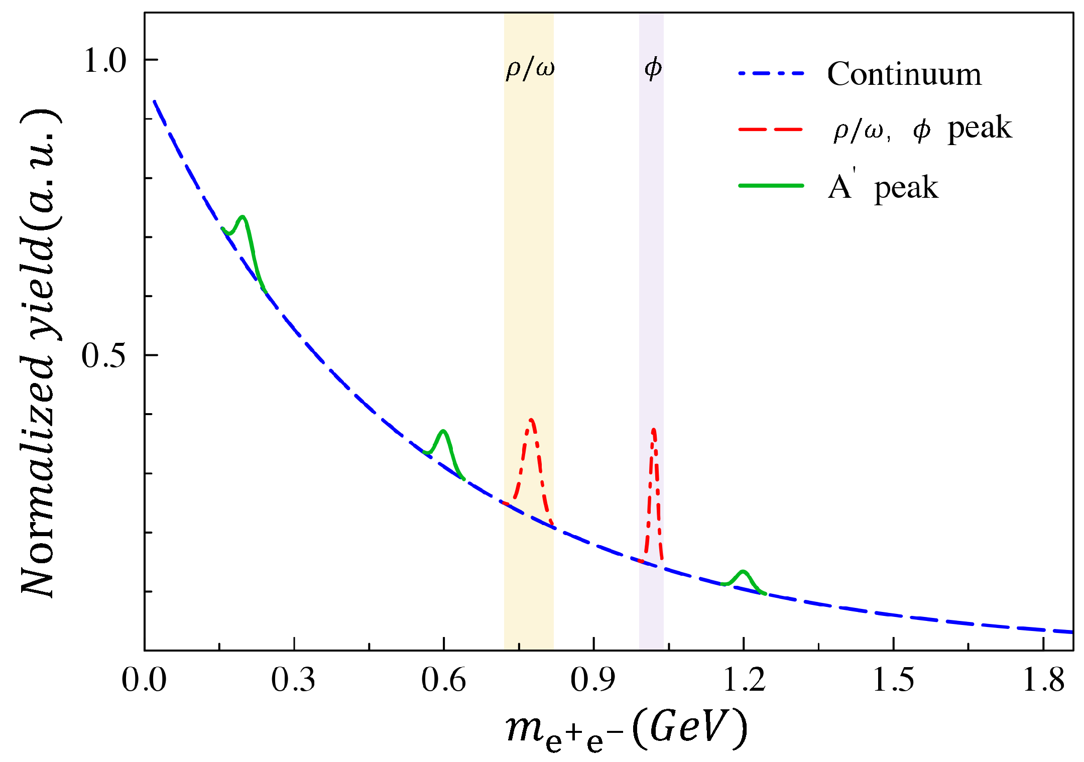
Table 1.
Representative values of the converted coupling reach in .
| [GeV] | |||
|---|---|---|---|
| 0.2 | |||
| 0.6 | |||
| 1.2 | |||
| 1.5 |
Table 2.
Positioning of this work relative to existing research perspectives.
| Research perspective | Core object | Main question | Relation to this work |
|---|---|---|---|
| Ordinary dark photon searches | versus ; visible or invisible decays | Production or decay through kinetic mixing | External context; not a direct constraint on the flavor changing charm amplitude. |
| Rare charm constraints | Branching fractions and Wilson coefficients | Deviation in rare processes | Closest in motivation; sensitive to long distance hadronic effects. |
| Standard Model background | spectrum and resonance templates | Continuum and vector meson backgrounds | Provides the background model, sidebands, and veto strategy. |
| This framework | , , , | Visible coupling reach from branching fraction sensitivity | Keeps hadronic normalization explicit and allows rescaling. |
Disclaimer/Publisher’s Note: The statements, opinions and data contained in all publications are solely those of the individual author(s) and contributor(s) and not of MDPI and/or the editor(s). MDPI and/or the editor(s) disclaim responsibility for any injury to people or property resulting from any ideas, methods, instructions or products referred to in the content. |
© 2026 by the authors. Licensee MDPI, Basel, Switzerland. This article is an open access article distributed under the terms and conditions of the Creative Commons Attribution (CC BY) license (http://creativecommons.org/licenses/by/4.0/).
Copyright: This open access article is published under a Creative Commons CC BY 4.0 license, which permit the free download, distribution, and reuse, provided that the author and preprint are cited in any reuse.


