Quantum Entanglement Beyond Kinematics: A Dynamical Hypothesis in (3,2)-Dimensional Spacetime

1. Introduction

Quantum entanglement is mathematically expressed through the non-factorizability of the wavefunction of a composite system. It implies the existence of correlated behaviors between entangled entities even when these are separated by an arbitrarily large distance and in the absence of any known physical connection. Entanglement is experimentally well established [2,3,4,5,6,7,8]. From a conceptual viewpoint, however, it remains puzzling because the formalism implies the existence of instantaneous correlations between spacelike separated events independently of their distance, in other words an underlying mediator, if it exists, must propagate at infinite velocity. This is at odds with traditional physical descriptions of interactions, since any action at a distance is always mediated by a physical actor (field, particle) constrained by relativistic locality.

The uneasiness with “spooky action at a distance,” as Einstein called quantum entanglement, had already been expressed, long before, by Isaac Newton with respect to gravity, who argued that matter could not act on matter “without the mediation of something else... through which their action and force may be transmitted” [9].

Newton’s remarks highlight an idea that has never faded in physics, that is, correlations must arise from interactions, and interactions need mediators.In this perspective, quantum nonlocality is conceptually bewildering precisely because it eludes this pattern: quantum mechanics provides correlation statistics with striking precision while leaving the causal structure opaque. Several attempts have been made to recover a mediator-based description by hypothesizing superluminal influences propagating at finite velocity $v>c$ [10,11,12,13,14]. Experimental bounds on such a signal velocity have been progressively improved, reaching $\sim {10}^{4}c$ [12], $\sim 5\times {10}^{6}c$ [13], and $\sim 3.3\times {10}^{4}c$ [14] in the CMB preferred frame, however the programme faces an obstruction of a different order altogether. These bounds concern detectability, not principle: quantum correlations cannot in any case be used to transmit controllable messages faster than light [15]. The deeper difficulty was identified by Bancal, Gisin et al. [16], who showed that any hidden-influence theory in which the mediator propagates at a superluminal but finite velocity necessarily implies operational superluminal signaling in suitable multipartite configurations, a conclusion that is in direct contradiction with Special Relativity and hinders finite-velocity mediation not merely experimentally but in principle.Their conclusion is: “[…] to keep no-signalling, […] quantum nonlocality must necessarily relate discontinuously parts of the universe that are arbitrarily distant. This gives further weight to the idea that quantum correlations somehow arise from outside spacetime, in the sense that no story in space and time can describe how they occur.” [16]. Although logically inescapable, this conclusion according to which a physical phenomenon originates outside of spacetime is disorienting and a source of conceptual uneasiness. A less problematic interpretation of the statement “arise from outside [ordinary] spacetime” is to assume that it signals the insufficiency of ordinary $(3,1)$-dimensional spacetime to encode the relevant causal structure and thus suggesting the replacement of the previous statement with “arise from inside an enlarged spacetime”. In other words we can try to recover a “causal” description of quantum nonlocality by assuming the existence of an extra time dimension so that two entangled objects can exchange a mediator at finite velocity in the $(3,2)$ dimensional bulk, while the projection of that exchange onto the $(3,1)$-dimensional spacetime, thus correlations, appear effectively instantaneous on the brane, respecting the no-signalling condition.

Hints in this direction come from the long-standing idea of representing Newtonian dynamics as geodesic motion in an extended spacetime, for example resorting to the Eisenhart lift, where the Hamiltonian flow of a mechanical system is encoded in the geodesics of a higher-dimensional Riemannian manifold [17,18,19]. In this geometric formulation, additional coordinates encode effective forces or correlations of the lower-dimensional theory.

This idea of introducing an additional temporal coordinate $\tau$ to ordinary $(3,1)$-dimensional spacetime has been put forward in Ref. [1]. In the framework of a $(3,2)$-dimensional spacetime it is hypothesized the existence of a field ${\mathcal{X}}_a(\mathbf{x},t,\tau )$ propagating at finite velocity along null geodesics of the enlarged spacetime and coupled to the wavefunction collapse dynamics at the endpoints of entanglement-based experiments. The wavefunction collapse is described by a modified version of the nonlinear, nonunitary evolution originally introduced by Bohm and Bub [20] where the field ${\mathcal{X}}_a(\mathbf{x},t,\tau )$ replaces random hidden variables.

The mention of two time dimensions immediately raises familiar concerns. Multiple-time theories are commonly associated with pathologies such as causality violations and ghostlike excitations [21,22]. These concerns are serious, but they are not uniformly fatal. It has been shown that the initial-value problem for ultrahyperbolic equations, with data posed on a hypersurface of mixed space- and timelike signature, can be rendered well posed after the imposition of a suitable nonlocal constraint on the data [23]. Weinstein further argued that deterministic and stable evolution can exist in theories with more than one time dimension and emphasised that such theories may exhibit “nonlocality without nonlocality”, namely nonlocal correlations without nonlocal causation [24]. That observation captures the central motivation of the present construction.

In the present work, these potential pathologies do not enter directly into the physical sector under study. The bulk field ${\mathcal{X}}_a$ is treated as an effective classical bulk physycal entity. Although the $(3,2)$ wave operator is ultrahyperbolic, an admissible sector is identified in which $\tau$-normalisability and vanishing flux restrict the bulk field to a family of effective four-dimensional Klein–Gordon modes, each governed on the brane by a standard hyperbolic equation with a well-defined retarded Green function [25]. Within this admissible sector the brane phenomenology is causally well defined, and the question of a global Cauchy problem for the full $(3,2)$ bulk does not arise.

The present work substantially develops the programme initiated in Ref. [1] by addressing several conceptual and fundamental issues left open there. We analyse a warped $(3,2)$-dimensional spacetime coupled to the bulk field ${\mathcal{X}}_a(\mathbf{x},t,\tau )$ and show that, within the metric ansatz adopted here, the five-dimensional vacuum General Relativity equations fix the warp factor uniquely up to sign and an additive constant. This is not a uniqueness theorem in the unrestricted space of five-dimensional solutions, but a fixation of the warp function within the adopted warped-product ansatz. We then show that the resulting geometrical framework is compatible with the standard causal structure on the brane and satisfies no-signaling in the linear-response phenomenology and, in the nonlinear collapse dynamics, reproduces the standard setting-independent marginals under conditions discussed explicitly in Section 5.4.

This article is organised as follows. Section 2 shows that an extra spatial dimension admits no effective superluminal shortcut on the brane, by an argument rooted in the causal structure of the warped metric. Section 3 introduces the warped $(3,2)$ geometry and derives the GR-selected warp factor. In Section 4 we analyse the null characteristics of the bulk wave equation and establish the existence of a null family with unbounded equal-time brane reach. Section 5 defines the brane-to-brane response through a t-retarded Green function, together with admissibility conditions in the extra-time direction.

Section 6 develops the dynamical model in four stages: the single-system Bohm–Bub collapse model (Section 6.1); its extension to a bipartite entangled system, introducing the crossed collapse ratios and the channel-normalised field (Section 6.2); the geometrisation of the two-source bulk mechanism, deriving the two-component contextual input from the $E=0$ geodesic kinematics (Section 6.3); and a retrospective translation table to the PRR toy model (Section 6.5). Contextual microstates and Born-rule recovery are treated in Section 6.4.

Section 7 specialises the framework to a photon pair and develops the two-pair cross-correlation prediction. Section 8 discusses experimental signatures, including a cross-pair Bell-test proposal and a parametric estimate of the signal magnitude. Section 9 gathers the concluding remarks and gives an explicit account of what is proved, what is assumed, and what remains open.

2. Can a (4,1)-Dimensional Spacetime Host a Dynamical Model of Quantum Entanglement?

The existence of extra dimensions, beyond the $3+1$ with which we perceive the physical world, has entered theoretical physics already one century ago with the formulation of the five-dimensional Kaluza-Klein theory (KKT), a classical field theory unifying gravitation and electromagnetism. With a few exotic exceptions [26,27], the additional spatial dimension in the KKT is compactified under the so-called cylinder condition, so that the extra dimension remains hidden at macroscopic scales. The Kaluza–Klein theory is considered a precursor of string theory, where resorting to extra space dimensions is deemed natural and necessary for mathematical consistency [28]. Also in these modern theories, the extra dimensions are typically curled up and microscopic, but their conceptual role is central.

Therefore, the idea of introducing an extra spatial dimension is not heretical, and under such an assumption a nonlocal behavior in $(3,1)$ dimensional spacetime can be seen as the projection of fully local phenomena in a higher-dimensional space. Actually, it has been surmised that entanglement and collapse phenomena could involve additional spatial dimensions, even if ordinary (Standard Model) quantum fields remain confined to $(3,1)$ dimensions. The author of Ref. [29] affirms one may surmise that “the usual fields only ‘live’ in $(3,1)$ dimensions, [whereas] the collapse involves also other dimensions, eventually being induced by ‘some field’ propagating also in these extra-dimensions.’’ In an extended geometry featuring an additional spatial direction entanglement correlations that appear instantaneous or acausal in $(3,1)$ spacetime could instead arise from ordinary, finite-velocity propagation in the higher-dimensional manifold.

Independent support for extra dimensions as a natural consequence of quantum mechanics comes from Brody and Graefe [30], who showed that quaternionic quantum mechanics for a spin-${\displaystyle \frac{1}{2}}$ particle requires the ambient physical space to have five dimensions, embedding standard three-dimensional dynamics as a canonical reduction. More recently, Furquan, Singh and Wesley [31] have independently proposed that a $(3,3)$-dimensional spacetime, motivated by a gravi-weak unification programme based on $E_8\otimes E_8$ octonion algebra, can resolve the EPR paradox by reinterpreting apparently spacelike-separated measurement events as timelike-separated events in the extended geometry, their framework also predicts a potential violation of the Tsirelson bound, a further observable distinction between extra-time and standard $(3,1)$ frameworks.

2.1. Randall–Sundrum Geometry in $(4,1)$ Dimensions and the Absence of Causal Shortcuts

The central question of this subsection is whether a warped extra spatial dimension can provide a causal mechanism for quantum correlations between spacelike-separated brane events. The answer is no: we prove that the Randall–Sundrum warp factor, far from shortening brane-to-brane travel times, strictly increases them relative to the brane-confined null geodesic. This result forces the move to a warped extra timelike dimension, which is the geometry developed in the remainder of this paper.

In a flat $(4,1)$-dimensional spacetime with

$$d{s}^2=g_{\mu \nu }d{x}^{\mu }d{x}^{\nu }+d{\zeta }^2,$$

(1)

where $g_{\mu \nu }=\mathrm{diag}(-c^2,+1,+1,+1)$, $x^{\mu }=(t,\mathbf{x})$, and $\zeta$ is the extra spatial coordinate, the brane-to-brane causal structure is identical to that of Minkowski space and no shortcut is possible. A nontrivial warp factor is therefore necessary, and we consider the Randall–Sundrum (RS) warped geometry [32,33]

$$d{s}^2=e^{-2f\left(\zeta \right)}{g}_{\mu \nu }d{x}^{\mu }d{x}^{\nu }+d{\zeta }^2,$$

(2)

in which our $(3,1)$ world is a hypersurface (brane) at $\zeta =0$. In the simplest RS configuration,

$$f\left(\zeta \right)=k\left|\zeta \right|,k>0,$$

(3)

with a ${\mathbb{Z}}_2$ symmetry across the brane. Note that $f\left(\zeta \right)\ge 0$ for all $\zeta$, a property used crucially below.

Let A and B be two events on the brane,

$$A=(t_A,{\mathbf{x}}_A,0),B=(t_B,{\mathbf{x}}_B,0),$$

with spatial separation $|{\mathbf{x}}_B-{\mathbf{x}}_A|$. A causal influence between A and B must follow a future-directed causal curve

$$\gamma \left(\lambda \right)=\left(t\left(\lambda \right),\mathbf{x}\left(\lambda \right),\zeta \left(\lambda \right)\right),$$

with $\gamma \left({\lambda }_1\right)=A$, $\gamma \left({\lambda }_2\right)=B$, and $d{s}^2\ge 0$ along $\gamma$.

For a null curve $(d{s}^2=0)$, Eq. (2) gives

$$0=e^{-2f\left(\zeta \right)}\left(-c^2{\dot{t}}^2+{\dot{\mathbf{x}}}^2\right)+{\dot{\zeta }}^2,$$

(4)

where dots denote differentiation with respect to $\lambda$. Rearranging,

$$c^2{\dot{t}}^2={\dot{\mathbf{x}}}^2+e^{2f\left(\zeta \right)}{\dot{\zeta }}^2,$$

(5)

and for future-directed propagation ($\dot{t}>0$),

$$\dot{t}={\displaystyle \frac{1}{c}}\sqrt{{\dot{\mathbf{x}}}^2+e^{2f\left(\zeta \right)}{\dot{\zeta }}^2}.$$

(6)

The coordinate travel time between the two brane events along $\gamma$ is therefore

$$T\left[\gamma \right]=t_B-t_A={\displaystyle \frac{1}{c}}{\int }_{{\lambda }_1}^{{\lambda }_2}\sqrt{{\dot{\mathbf{x}}}^2+e^{2f\left(\zeta \right)}{\dot{\zeta }}^2}d\lambda .$$

(7)

Since $f\left(\zeta \right)\ge 0$ we have $e^{2f\left(\zeta \right)}\ge 1$, so the integrand satisfies

$$\sqrt{{\dot{\mathbf{x}}}^2+e^{2f\left(\zeta \right)}{\dot{\zeta }}^2}\ge \sqrt{{\dot{\mathbf{x}}}^2+{\dot{\zeta }}^2}\ge \left|\dot{\mathbf{x}}\right|,$$

(8)

which implies

$$T\left[\gamma \right]\ge {\displaystyle \frac{1}{c}}{\int }_{{\lambda }_1}^{{\lambda }_2}\left|\dot{\mathbf{x}}\right|d\lambda .$$

(9)

The right-hand side is the arc length of the spatial projection $\mathbf{x}\left(\lambda \right)$ in ${\mathbb{R}}^3$, which satisfies the triangle inequality

$${\int }_{{\lambda }_1}^{{\lambda }_2}|\dot{\mathbf{x}}|d\lambda \ge |{\mathbf{x}}_B-{\mathbf{x}}_A|,$$

(10)

with equality if and only if $\mathbf{x}\left(\lambda \right)$ is a straight line with constant direction. Hence

$$T\left[\gamma \right]\ge {\displaystyle \frac{|{\mathbf{x}}_B-{\mathbf{x}}_A|}{c}}.$$

(11)

Uniqueness of the saturating path. Equality in (11) requires simultaneously that $\dot{\zeta }=0$ almost everywhere, so the curve stays on the brane, and that $\mathbf{x}\left(\lambda \right)$ is a straight segment traversed at constant speed. The first condition is necessary because whenever $\dot{\zeta }\ne 0$ on a set of positive measure, the integrand satisfies $\sqrt{{\dot{\mathbf{x}}}^2+e^{2f}{\dot{\zeta }}^2}>\sqrt{{\dot{\mathbf{x}}}^2+{\dot{\zeta }}^2}\ge \left|\dot{\mathbf{x}}\right|$ strictly (since $e^{2f}\ge 1>0$), so integrating gives $T\left[\gamma \right]>|{\mathbf{x}}_B-{\mathbf{x}}_A|/c$. The unique null path saturating (11) is therefore the brane-confined Minkowski null geodesic

$$\mathbf{x}\left(\lambda \right)={\mathbf{x}}_A+{\displaystyle \frac{\lambda -{\lambda }_1}{{\lambda }_2-{\lambda }_1}}\left({\mathbf{x}}_B-{\mathbf{x}}_A\right),$$

(12)

whose affine parametrisation keeps $\dot{\mathbf{x}}$ at constant direction and magnitude, exactly saturating the triangle inequality (11). The minimum travel time is

$$T_{min}={\displaystyle \frac{|{\mathbf{x}}_B-{\mathbf{x}}_A|}{c}}.$$

(13)

One might expect a path cutting through the bulk to save travel time by traversing a shorter coordinate distance between A and B. The warp factor says otherwise. Any bulk excursion, any segment where $\dot{\zeta }\ne 0$, contributes a term $e^{2f\left(\zeta \right)}{\dot{\zeta }}^2$ to the integrand of $T\left[\gamma \right]$ (7), and since $f\left(\zeta \right)=k\left|\zeta \right|\ge 0$ this contribution is strictly positive and grows exponentially with the depth $\left|\zeta \right|$ of the excursion. Dipping into the bulk costs more time, not less. The brane-confined null geodesic is the unique path that avoids this penalty entirely; it is, for that reason, the sole minimiser of (11).

This lower-bound argument, together with the explicit mechanism above, proves that in symmetric Randall–Sundrum warping every 5D null geodesic projects onto a causal 4D path: the projected velocity satisfies $|d\mathbf{x}/dt|\le c$ at all times. Two distant brane points may well look geometrically closer through the bulk embedding, but the causal structure of the warped metric turns that apparent proximity into a strictly greater time cost. The bulk is not a shortcut, it is a detour.

3. Extending Spacetime to (3,2) Dimensions

Introducing an additional time dimension raises well-known theoretical concerns: generic field theories on a $(3,2)$ background can suffer from ill-posed Cauchy problems, violations of causality, and ghost instabilities [23,24]. We show in the following that these pathologies can be avoided within a physically admissible sector of the theory, defined by appropriate conditions on the bulk field profiles and the brane-time Green function.

3.1. Asymmetric Warping in the $(3,2)$ Case

In the Appendix of our previous work [1], we briefly remarked that a construction suggested by Visser [27] for exotic Kaluza–Klein models could be adapted to a five-dimensional spacetime of signature $(-,+,+,+,-)$, i.e. a $(3,2)$ geometry with a noncompact extra time dimension. Following that approach, we considered a warped line element in which only the physical time coordinate is multiplied by a warp factor depending on the second temporal coordinate $\tau$, while the spatial part of the induced $(3,1)$ metric remains unwarped. That discussion was intentionally limited to a qualitative indication of how such a geometry might trap ordinary fields on the four-dimensional spacetime while allowing the extra time direction to play a hidden dynamical role. No attempt was made to examine the corresponding Einstein equations, the consistency of the causal structure, or the physical viability of the resulting warp factor. The Appendix concluded with the explicit remark that “how to choose such a metric and how to choose a suitable and physically meaningful function $f\left(\tau \right)$ remain far beyond the aim of the present work.”

Here we address precisely this point left open previously. Our goal is to determine whether a purely time–warped $(3,2)$ metric can provide a consistent and physically meaningful geometric framework for a dynamical mechanism underlying quantum nonlocality. We therefore analyze the geometry

$$d{s}^2=-e^{-2f\left(\tau \right)}{c}^{2}d{t}^2+d{\mathbf{x}}^2-w^{2}d{\tau }^2,$$

(14)

which represents a purely time-warped $(3,2)$ spacetime: the warp factor modifies only the temporal component of the induced $(3,1)$ metric, while the spatial directions remain unwarped. However, we show below that it cannot provide a satisfactory geometric basis for a dynamical account of entanglement correlations.

Curvature and Einstein Equations

For the metric (14), the nonzero metric components and their inverses are

$$\begin{array}{ccc}\hfill g_{tt}& =& -c^2{e}^{-2f},g_{ij}={\delta }_{ij},g_{\tau \tau }=-w^2,\hfill \\ \hfill g^{tt}& =& -{\displaystyle \frac{e^{2f}}{c^2}},g^{ij}={\delta }^{ij},g^{\tau \tau }=-{\displaystyle \frac{1}{w^2}}.\hfill \end{array}$$

The only nontrivial $\tau$-dependence occurs in $g_{tt}$; using the conventions of Section 3.2 [34], the only nonvanishing Christoffel symbols are

$${{\Gamma }^t}_{t_{\tau }}={{\Gamma }^t}_{{\tau }_t}={\displaystyle \frac{1}{2}}{g}^{tt}{\partial }_{\tau }{g}_{tt}={\displaystyle \frac{1}{2}}\left(-{\displaystyle \frac{e^{2f}}{c^2}}\right)\left(2c^2{f}^{\prime }{e}^{-2f}\right)=-f^{\prime }\left(\tau \right),$$

$$\begin{array}{ccc}\hfill {{\Gamma }^{\tau }}_{t_t}& =& -{\displaystyle \frac{1}{2}}{g}^{\tau \tau }{\partial }_{\tau }{g}_{tt}=-{\displaystyle \frac{1}{2}}\left(-{\displaystyle \frac{1}{w^2}}\right)\left(2c^2{f}^{\prime }{e}^{-2f}\right)\hfill \\ & =& +{\displaystyle \frac{c^2}{w^2}}{e}^{-2f\left(\tau \right)}{f}^{\prime }\left(\tau \right).\hfill \end{array}$$

The corresponding Ricci tensor components, computed directly from the Christoffel symbols above, are

$$\begin{array}{cc}\hfill R_{tt}& ={\partial }_{\tau }{{\Gamma }^{\tau }}_{t_t}+{{\Gamma }^{\mu }}_{{\mu }_{\tau }}{{\Gamma }^{\tau }}_{t_t}-{{\Gamma }^{\mu }}_{t_{\tau }}{{\Gamma }^{\tau }}_{{\mu }_t}={\displaystyle \frac{c^2{e}^{-2f}}{w^2}}\left(2f^{\prime 2}-f^{\prime \prime }\right),\hfill \\ \hfill R_{ij}& =0,\hfill \\ \hfill R_{\tau \tau }& =\left(f^{\prime \prime }-f^{\prime 2}\right),\hfill \end{array}$$

and the scalar curvature $R=g^{AB}{R}_{AB}$ is

$$\begin{array}{ccc}\hfill R=g^{tt}{R}_{tt}+g^{\tau \tau }{R}_{\tau \tau }& =& \left(-{\displaystyle \frac{e^{2f}}{c^2}}\right){\displaystyle \frac{c^2{e}^{-2f}}{w^2}}(2f^{\prime 2}-f^{\prime \prime })\hfill \\ & +& \left(-{\displaystyle \frac{1}{w^2}}\right)(f^{\prime \prime }-f^{\prime 2})=-{\displaystyle \frac{f^{\prime 2}}{w^2}}.\hfill \end{array}$$

The Einstein tensor $G_{AB}=R_{AB}-\frac{1}{2}{g}_{AB}R$ then has components

$$\begin{array}{ccc}\hfill G_{tt}& =& {\displaystyle \frac{c^2{e}^{-2f}}{w^2}}\left(2f^{\prime 2}-f^{\prime \prime }\right)-{\displaystyle \frac{1}{2}}(-c^2{e}^{-2f})\left(-{\displaystyle \frac{f^{\prime 2}}{w^2}}\right)\hfill \\ & =& {\displaystyle \frac{c^2{e}^{-2f}}{w^2}}\left({\displaystyle \frac{3}{2}}{f}^{\prime 2}-f^{\prime \prime }\right),\hfill \\ \hfill G_{ij}& =& -{\displaystyle \frac{1}{2}}{\delta }_{ij}\left(-{\displaystyle \frac{f^{\prime 2}}{w^2}}\right)={\displaystyle \frac{f^{\prime 2}}{2w^2}}{\delta }_{ij},\hfill \\ \hfill G_{\tau \tau }& =& (f^{\prime \prime }-f^{\prime 2})-{\displaystyle \frac{1}{2}}(-w^2)\left(-{\displaystyle \frac{f^{\prime 2}}{w^2}}\right)=f^{\prime \prime }-{\displaystyle \frac{3}{2}}{f}^{\prime 2}.\hfill \end{array}$$

Imposing the vacuum Einstein equations with cosmological constant,

$$G_{AB}+{\Lambda }_5{g}_{AB}=0,$$

(15)

the three independent components yield

$$\begin{array}{ccc}\hfill \left(tt\right):& & {\displaystyle \frac{c^2{e}^{-2f}}{w^2}}\left(\frac{3}{2}{f}^{\prime 2}-f^{\prime \prime }\right)-{\Lambda }_5{c}^2{e}^{-2f}=0\hfill \end{array}$$

$$\begin{array}{ccc}& & ⟹{\Lambda }_5={\displaystyle \frac{1}{w^2}}\left(\frac{3}{2}{f}^{\prime 2}-f^{\prime \prime }\right),\hfill \end{array}$$

(16)

$$\begin{array}{ccc}\hfill \left(ij\right):& & {\displaystyle \frac{f^{\prime 2}}{2w^2}}+{\Lambda }_5=0⟹{\Lambda }_5=-{\displaystyle \frac{f^{\prime 2}}{2w^2}},\hfill \\ \hfill \left(\tau \tau \right):& & \left(f^{\prime \prime }-\frac{3}{2}{f}^{\prime 2}\right)-{\Lambda }_5{w}^2=0\hfill \end{array}$$

(17)

$$\begin{array}{ccc}& & ⟹{\Lambda }_5={\displaystyle \frac{f^{\prime \prime }-\frac{3}{2}{f}^{\prime 2}}{w^2}}.\hfill \end{array}$$

(18)

Equations (16) and (17) must hold simultaneously:

$$\frac{3}{2}{f}^{\prime 2}-f^{\prime \prime }=-\frac{1}{2}{f}^{\prime 2}⟹f^{\prime \prime }=2f^{\prime 2}.$$

(19)

Equations (17) and (18) must also hold simultaneously:

$$-\frac{1}{2}{f}^{\prime 2}=f^{\prime \prime }-\frac{3}{2}{f}^{\prime 2}⟹f^{\prime \prime }=f^{\prime 2}.$$

(20)

Equations (19) and (20) are simultaneously satisfiable only if $f^{\prime 2}=0$, i.e. $f\left(\tau \right)=\mathrm{const}$. The vacuum Einstein equations therefore admit no nonconstant solution for the pure time-warp ansatz (14), for any value of ${\Lambda }_5$. A constant f is trivially equivalent (by rescaling t) to $f=0$, giving ordinary five-dimensional Minkowski space. Consequently, such a pure time warp cannot generate an invariant geometric effect and therefore cannot supply genuine causal “shortcuts” on the brane. In this sense, pure time warping is dynamically trivial in General Relativity and cannot provide the geometric basis for the entanglement-correlation mechanism pursued here.We now turn to a setting where this idea can be implemented consistently, namely a symmetrically warped $(3,2)$-dimensional spacetime.

3.2. Modelling the Extended Spacetime Geometry with Symmetric Warping

Specifically, we consider a metric in which the extra time coordinate $\tau$ enters through a $\tau$-dependent warp factor. A minimal extension of the Randall–Sundrum form can be written as

$$d{s}^2=e^{-2f\left(\tau \right)}{\eta }_{\mu \nu }d{x}^{\mu }d{x}^{\nu }-w^{2}d{\tau }^2,$$

(21)

where ${\eta }_{\mu \nu }=\mathrm{diag}(-c^2,+1,+1,+1)$, w has dimensions of velocity, $f\left(\tau \right)$ is a warping function depending only on the extra timelike coordinate $\tau$, and sets the scale of propagation in the extra–time direction. We take $\tau$ to be of noncompact support, $\tau \in (-\infty ,+\infty )$. For clarity, we now provide computational details showing that the metric (21) admits a simple bulk solution of the five-dimensional Einstein equations with a cosmological constant, and we determine the corresponding analytic form of $f\left(\tau \right)$. We rewrite (21) as

$$d{s}^2=g_{AB}d{x}^{A}d{x}^B,$$

(22)

with coordinates $x^A=(x^{\mu },\tau )$, $A=0,1,2,3,\tau$. The nonvanishing components of the metric are

$$g_{\mu \nu }=e^{-2f\left(\tau \right)}{\eta }_{\mu \nu },g_{\tau \tau }=-w^2,g_{\mu \tau }=g_{\tau \mu }=0,$$

(23)

and the inverse metric is

$$g^{\mu \nu }=e^{2f\left(\tau \right)}{\eta }^{\mu \nu },g^{\tau \tau }=-{\displaystyle \frac{1}{w^2}},g^{\mu \tau }=g^{\tau \mu }=0.$$

(24)

The only nonzero derivative of $g_{AB}$ is with respect to $\tau$,

$${\partial }_{\tau }{g}_{\mu \nu }=-2f^{\prime }\left(\tau \right)e^{-2f\left(\tau \right)}{\eta }_{\mu \nu }=-2f^{\prime }\left(\tau \right)g_{\mu \nu },$$

(25)

where a prime denotes $d/d\tau$. All derivatives with respect to $x^{\mu }$ vanish:

$${\partial }_{\mu }{g}_{AB}=0,\forall A,B,\mu =0,1,2,3.$$

(26)

The Christoffel coefficients are

$${{\Gamma }^A}_{B_C}={\displaystyle \frac{1}{2}}{g}^{AD}\left({\partial }_B{g}_{CD}+{\partial }_C{g}_{BD}-{\partial }_D{g}_{BC}\right).$$

(27)

Using the metric above and the fact that $f=f\left(\tau \right)$, one finds that the only nonvanishing components are

$$\begin{array}{cc}\hfill {{\Gamma }^{\rho }}_{{\mu }_{\tau }}& ={{\Gamma }^{\rho }}_{{\tau }_{\mu }}=-f^{\prime }\left(\tau \right){{\delta }^{\rho }}_{\mu },\hfill \end{array}$$

(28)

$$\begin{array}{cc}\hfill {{\Gamma }^{\tau }}_{{\mu }_{\nu }}& =-{\displaystyle \frac{f^{\prime }\left(\tau \right)}{w^2}}{g}_{\mu \nu }=-{\displaystyle \frac{f^{\prime }\left(\tau \right)}{w^2}}{e}^{-2f\left(\tau \right)}{\eta }_{\mu \nu }.\hfill \end{array}$$

(29)

All other components ${{\Gamma }^A}_{B_C}$ vanish.

The Ricci tensor is defined as

$$R_{AB}={\partial }_C{{\Gamma }^C}_{A_B}-{\partial }_B{{\Gamma }^C}_{A_C}+{{\Gamma }^C}_{A_B}{{\Gamma }^D}_{C_D}-{{\Gamma }^C}_{A_D}{{\Gamma }^D}_{B_C}.$$

(30)

Given that all dependence is on $\tau$ alone, and using (28)–(29), the nonvanishing Ricci components are:

$$R_{\mu \nu }={\displaystyle \frac{4f^{\prime }{\left(\tau \right)}^2-f^{\prime \prime }\left(\tau \right)}{w^2}}{g}_{\mu \nu }={\displaystyle \frac{4f^{\prime 2}-f^{\prime \prime }}{w^2}}{e}^{-2f\left(\tau \right)}{\eta }_{\mu \nu },$$

(31)

and

$$R_{\tau \tau }=4f^{\prime \prime }\left(\tau \right)-4f^{\prime }{\left(\tau \right)}^2.$$

(32)

The mixed components vanish identically by the warped-product structure of the metric:

$$R_{\mu \tau }=R_{\tau \mu }=0,G_{\mu \tau }=G_{\tau \mu }=0.$$

(33)

This is an algebraic consequence of the metric ansatz (21), not a consequence of the field equations: the Christoffel symbols (28)–(29) contain no mixed $(\mu ,\tau )$ terms, so the corresponding Ricci and Einstein components vanish before any field equation is imposed.

The scalar curvature is

$$R=g^{AB}{R}_{AB}=g^{\mu \nu }{R}_{\mu \nu }+g^{\tau \tau }{R}_{\tau \tau }.$$

(34)

Using $g^{\mu \nu }{g}_{\mu \nu }=4$ and $g^{\tau \tau }=-1/w^2$, and substituting (31) and (32), we obtain

$$\begin{array}{cc}\hfill g^{\mu \nu }{R}_{\mu \nu }& ={\displaystyle \frac{16f^{\prime 2}-4f^{\prime \prime }}{w^2}},\hfill \end{array}$$

(35)

$$\begin{array}{cc}\hfill g^{\tau \tau }{R}_{\tau \tau }& =-{\displaystyle \frac{1}{w^2}}\left(4f^{\prime \prime }-4f^{\prime 2}\right).\hfill \end{array}$$

(36)

Therefore,

$$R={\displaystyle \frac{4}{w^2}}\left(5f^{\prime 2}-2f^{\prime \prime }\right).$$

(37)

The Einstein tensor is

$$G_{AB}=R_{AB}-{\displaystyle \frac{1}{2}}{g}_{AB}R.$$

(38)

Using (31) and (37), the brane components are

$$\begin{array}{cc}\hfill G_{\mu \nu }& =R_{\mu \nu }-\frac{1}{2}{g}_{\mu \nu }R={\displaystyle \frac{3}{w^2}}\left(f^{\prime \prime }\left(\tau \right)-2f^{\prime }{\left(\tau \right)}^2\right)g_{\mu \nu },\hfill \end{array}$$

(39)

and using (32), (37), and $g_{\tau \tau }=-w^2$, the extra-time component is

$$\begin{array}{cc}\hfill G_{\tau \tau }& =R_{\tau \tau }-\frac{1}{2}{g}_{\tau \tau }R=6f^{\prime }{\left(\tau \right)}^2.\hfill \end{array}$$

(40)

The mixed components $G_{\mu \tau }=G_{\tau \mu }=0$ vanish identically, as established above for $R_{\mu \tau }$.

Einstein Equations and the Warp Factor $f\left(\tau \right)$

We now impose the validity of the five-dimensional Einstein equations with a bulk cosmological constant ${\Lambda }_5$ and no matter sources in the bulk (i.e. away from any brane-localized stress tensor),

$$G_{AB}+{\Lambda }_5{g}_{AB}=0.$$

(41)

From (40) and $g_{\tau \tau }=-w^2$ we have

$$G_{\tau \tau }+{\Lambda }_5{g}_{\tau \tau }=6f^{\prime 2}-{\Lambda }_5{w}^2=0,$$

(42)

so

$$f^{\prime }{\left(\tau \right)}^2={\displaystyle \frac{{\Lambda }_5{w}^2}{6}}.$$

(43)

This requires ${\Lambda }_5>0$ and implies that $f^{\prime }\left(\tau \right)$ is constant in the bulk:

$$f^{\prime }\left(\tau \right)=k,k=\pm w\sqrt{{\displaystyle \frac{{\Lambda }_5}{6}}}.$$

(44)

From (39) and $g_{\mu \nu }=e^{-2f}{\eta }_{\mu \nu }$, the $\left(\mu \nu \right)$ component of (41) reads

$${\displaystyle \frac{3}{w^2}}\left(f^{\prime \prime }-2f^{\prime 2}\right)g_{\mu \nu }+{\Lambda }_5{g}_{\mu \nu }=0,$$

(45)

which reduces to

$$f^{\prime \prime }-2f^{\prime 2}+{\displaystyle \frac{{\Lambda }_5{w}^2}{3}}=0.$$

(46)

Using (43), ${\Lambda }_5{w}^2/3=2f^{\prime 2}$, hence (46) gives

$$f^{\prime \prime }\left(\tau \right)=0,$$

(47)

consistent with constant $f^{\prime }$. Integrating in the bulk,

$$f\left(\tau \right)=k\tau +f_0,k=\pm w\sqrt{{\displaystyle \frac{{\Lambda }_5}{6}}},$$

(48)

with $f_0$ an integration constant that can be absorbed into a rescaling of the four-dimensional coordinates. Thus, in the bulk the warped $(3,2)$ metric (22) is supported by a positive cosmological constant ${\Lambda }_5$.

If a ${\mathbb{Z}}_2$-symmetric thin brane is inserted at $\tau =0$, the Israel junction condition [35] fixes the sign of k on either side of the brane, yielding the standard kink profile

$$f\left(\tau \right)=k\left|\tau \right|,k=w\sqrt{{\displaystyle \frac{{\Lambda }_5}{6}}},$$

(49)

so that the warp factor becomes $e^{-2f\left(\tau \right)}=e^{-2k\left|\tau \right|}$ (f is then only piecewise smooth).

Since $\tau$ is a timelike coordinate with dimensions of time, the warping constant k has dimensions of inverse time (${\mathrm{s}}^{-1}$). It plays the role of the inverse curvature scale of the bulk, analogous to $k_{\mathrm{RS}}\sim 1/L_{\mathrm{AdS}}$ in the Randall–Sundrum model, with the replacement $L_{\mathrm{AdS}}\to c/k$.

Remark.

Let us emphasize that the metric (21) with warp factor (49) is an admissible ansatz for the geometric structure of a $(3,2)$-dimensional spacetime because it satisfies the equations of General Relativity.

Remark on the sign of ${\Lambda }_5$ and the nature of the bulk.

The warp function $f\left(\tau \right)=k\left|\tau \right|$ and the localisation mechanism are formally identical to RS, but the positive sign of ${\Lambda }_5$ is a direct consequence of the timelike signature of the extra dimension and distinguishes the present framework from the Anti-de Sitter bulk of the standard RS model.

3.3. Introducing a Massless Information-Carrying Field ${\mathcal{X}}_a(x,\tau )$

As shown in Section 4, bulk null geodesics in the symmetrically warped metric (21) can project onto the $(3,1)$ brane with arbitrarily large effective velocities between pairs of brane events. This provides a natural setting for modeling quantum correlations as mediated by a massless bulk field ${\mathcal{X}}_a(x,\tau )$, where $x=(\mathbf{x},t)$, with internal index $a=1,\dots ,N$, propagating in the warped $(3,2)$ geometry (21). “Massless” here means that no bulk mass term $M^2{\mathcal{X}}_a^2$ is included in the action. The characteristic structure is therefore governed by the metric principal part ${\square }_{(3,2)}$: in the geometric–optics limit the characteristics lie on the bulk null cone. Measurement events on the brane act as sources localized at $\tau =0$.

Remark.

The label a stands for internal degrees of freedom and is not a spacetime index. One may view ${\mathcal{X}}_a$ as an ensemble of scalar fields obeying the same five-dimensional propagation equation. The multiplicity N has nothing to do with the geometric construction, it just counts the number of independent collapse-driving channels. A minimal choice is of course $N=1$ sufficient for a two-outcome measurement. For a d-outcome measurement one may take $N=d$ so that each component ${\mathcal{X}}_a$ drives a distinct outcome channel, without qualitative change of the predicted outcome statistics. Throughout this paper ${\mathcal{X}}_a$ is treated as a classical bulk field that satisfies a classical wave equation, and quantum correlations enter only through a suitably defined ensemble distribution $\rho \left(\lambda \right)$ over classical field configurations (Section 5 and the subsection on response vs. correlations therein).

3.3.1. Action and Field Equation

The minimally coupled bulk action for the bulk field ${\mathcal{X}}_a(x,\tau )$, sourced by a brane-localized current $J_a\left(x\right)$ at $\tau =0$, is

$$\begin{array}{ccc}\hfill S\left[\mathcal{X}\right]& =& {\displaystyle \frac{1}{2}}\int d^{4}xd\tau \sqrt{\left|g\right|}{g}^{AB}{\partial }_A{\mathcal{X}}_a{\partial }_B{\mathcal{X}}_a\hfill \\ & & +\kappa \int d^{4}xd\tau \sqrt{\left|g\right|}{J}_a\left(x\right)\delta \left(\tau \right){\mathcal{X}}_a(x,\tau ),\hfill \end{array}$$

(50)

where summation over the internal index a is understood. Varying S yields the sourced wave equation, where ${\square }_5$ is the Laplace–Beltrami operator [34]

$${\square }_5{\mathcal{X}}_a\equiv {\displaystyle \frac{1}{\sqrt{\left|g\right|}}}{\partial }_A\left(\sqrt{\left|g\right|}{g}^{AB}{\partial }_B{\mathcal{X}}_a\right)=+\kappa J_a\left(x\right)\delta \left(\tau \right).$$

(51)

For the warped metric $d{s}^2=e^{-2f\left(\tau \right)}{\eta }_{\mu \nu }d{x}^{\mu }d{x}^{\nu }-w^{2}d{\tau }^2$, Eq. (51) becomes

$$-{\displaystyle \frac{1}{w^2}}{\partial }_{\tau }\left(e^{-4f}{\partial }_{\tau }{\mathcal{X}}_a\right)+e^{-2f}{\square }_4{\mathcal{X}}_a=+\kappa e^{-4f}{J}_a\left(x\right)\delta \left(\tau \right),$$

(52)

with ${\square }_4={\eta }^{\mu \nu }{\partial }_{\mu }{\partial }_{\nu }$. The positive sign on the right-hand side of (52) follows directly from the $+\kappa$ source term in the action (50). Integrating Eq. (52) across a narrow interval around $\tau =0$ gives the brane matching (jump) condition

$$\begin{array}{ccc}\hfill {\left[{\partial }_{\tau }{\mathcal{X}}_a(x,\tau )\right]}_{0^{-}}^{0^{+}}& \equiv & {\partial }_{\tau }{\mathcal{X}}_a(x,0^{+})-{\partial }_{\tau }{\mathcal{X}}_a(x,0^{-})\hfill \\ & =& -w^2\kappa J_a\left(x\right).\hfill \end{array}$$

(53)

Equation (53) makes precise in what sense the brane source injects a bulk disturbance: under standard regularity assumptions the field ${\mathcal{X}}_a$ itself is continuous at $\tau =0$, while its normal derivative has a discontinuity fixed by the source strength.

3.3.2. Separation Along the Brane and Spectral Resolution in $\tau$

Since the background depends only on $\tau$, the brane directions t and $\mathbf{x}$ are Killing directions and a Fourier decomposition along the brane is natural,

$$\mathcal{X}(x,\tau )=\int {\displaystyle \frac{d\omega d^3\mathbf{k}}{{\left(2\pi \right)}^4}}{e}^{-i\omega t+i\mathbf{k}·\mathbf{x}}{\psi }_{\omega ,\mathbf{k}}\left(\tau \right),$$

(54)

which reduces the bulk wave equation (away from $\tau =0$) to a second-order ODE in $\tau$ with $(\omega ,\mathbf{k})$ as parameters,

$${\psi }^{\prime \prime }-4f^{\prime }{\psi }^{\prime }+w^2{e}^{+2f\left(\tau \right)}\left({\mathbf{k}}^2-{\displaystyle \frac{{\omega }^2}{c^2}}\right)\psi =0,(\tau \ne 0).$$

(55)

The bulk wave equation is diagonal in the internal index a, so the geometry does not mix different components; Eq. (55) holds for each component of ${\mathcal{X}}_a$ separately. Throughout this section the index a is suppressed: $\mathcal{X}$, $\psi$, and $\varphi$ denote any single component, and the full field is recovered by restoring a.

A plane-wave ansatz $e^{iq\tau }$ does not diagonalize the $\tau$-dependence, because the warp factor $f\left(\tau \right)$ breaks $\tau$-translation invariance and the coefficients in (55) depend explicitly on $\tau$. The standard approach is to recast the problem as an eigenvalue equation for the self-adjoint Sturm–Liouville operator in $\tau$ induced by the warp factor, whose normalizable eigenfunctions play the role of plane waves in the flat case.

Concretely, inserting the separated ansatz $\mathcal{X}(x,\tau )=\varphi \left(x\right)\psi \left(\tau \right)$ into the bulk wave equation (52) and dividing through by $\varphi \left(x\right)\psi \left(\tau \right)$ splits the left-hand side into a function of x alone and a function of $\tau$ alone. The two sides must therefore each equal the same constant, the separation constant, written as $-{\mu }^2$ with the sign chosen so that ${\mu }^2\ge 0$ corresponds to a real 4D mass. This yields two decoupled equations: the $\tau$-equation

$$-{\displaystyle \frac{1}{w^2}}{\displaystyle \frac{d}{d\tau }}\left(e^{-4f\left(\tau \right)}{\displaystyle \frac{d\psi }{d\tau }}\right)={\mu }^2{e}^{-2f\left(\tau \right)}\psi ,$$

(56)

and the four-dimensional equation $({\square }_4+{\mu }^2)\varphi =0$, in which ${\mu }^2$ is the squared 4D mass of the mode.

Equation (56) is of Sturm–Liouville type [36],

$$\begin{array}{ccc}\hfill -{\displaystyle \frac{d}{d\tau }}\left(p\left(\tau \right){\psi }^{\prime }\left(\tau \right)\right)& =& \lambda W\left(\tau \right)\psi \left(\tau \right),\hfill \\ \hfill p\left(\tau \right)& =& {\displaystyle \frac{1}{w^2}}{e}^{-4f\left(\tau \right)},\lambda ={\mu }^2,\hfill \end{array}$$

(57)

and therefore fixes the warped weight as

$$W\left(\tau \right)=e^{-2f\left(\tau \right)}.$$

(58)

This weight is the function with respect to which the $\tau$-operator is self-adjoint. Equivalently, it is the measure that appears in the bulk kinetic term when one inserts a separated ansatz into the action. Indeed, starting from the bulk kinetic term

$$S_{\mathrm{kin}}=-{\displaystyle \frac{1}{2}}\int d^{4}xd\tau \sqrt{\left|g\right|}\left[g^{\mu \nu }{\partial }_{\mu }\mathcal{X}{\partial }_{\nu }\mathcal{X}+g^{\tau \tau }{\left({\partial }_{\tau }\mathcal{X}\right)}^2\right],$$

(59)

and inserting the separated ansatz $\mathcal{X}(x,\tau )=\varphi \left(x\right)\psi \left(\tau \right)$, the two terms decouple: the $\tau$-kinetic term $g^{\tau \tau }{\left({\partial }_{\tau }\psi \right)}^2{\varphi }^2$ contributes to the eigenvalue equation for $\psi \left(\tau \right)$ but not to the 4D kinetic normalization of $\varphi \left(x\right)$. The brane-direction term yields

$$S_{\mathrm{kin}}^{\left(4\right)}=-{\displaystyle \frac{1}{2}}\int d^{4}x\left({\partial }_{\mu }\varphi \right)\left({\partial }^{\mu }\varphi \right)\underset{=1(\mathrm{canonical}\mathrm{normalization})}{\underbrace{\int d\tau \sqrt{\left|g\right|}{g}^{\mu \nu }\psi {\left(\tau \right)}^2}},$$

(60)

so that $\varphi \left(x\right)$ has a canonically normalized 4D kinetic term once the mode normalization condition is imposed.

For the warped metric (21) one has $\sqrt{\left|g\right|}{g}^{\mu \nu }\propto e^{-4f\left(\tau \right)}·e^{2f\left(\tau \right)}=e^{-2f\left(\tau \right)}\equiv W\left(\tau \right)$, hence the induced four-dimensional kinetic term carries the overall factor

$$\int d\tau W\left(\tau \right)\psi {\left(\tau \right)}^2,$$

(61)

which is therefore the kinetic norm and the criterion for normalizability.

Remark on dimensions.

With the standard five-dimensional kinetic term, each component ${\mathcal{X}}_a$ has dimension $\left[{\mathcal{X}}_a\right]\sim L^{-3/2}$ in $\hslash =c=1$ units.

If ${\psi }_n$ and ${\psi }_m$ are eigenfunctions with eigenvalues ${\mu }_n^2$ and ${\mu }_m^2$, they satisfy the Sturm–Liouville equations

$$\begin{array}{ccc}\hfill -{\displaystyle \frac{d}{d\tau }}\left(p\left(\tau \right){\psi }_n^{\prime }\left(\tau \right)\right)& =& {\mu }_n^{2}W\left(\tau \right){\psi }_n\left(\tau \right),\hfill \\ \hfill -{\displaystyle \frac{d}{d\tau }}\left(p\left(\tau \right){\psi }_m^{\prime }\left(\tau \right)\right)& =& {\mu }_m^{2}W\left(\tau \right){\psi }_m\left(\tau \right).\hfill \end{array}$$

(62)

Multiplying the first equation in (62) by ${\psi }_m$ and the second by ${\psi }_n$ gives

$$\begin{array}{ccc}\hfill -{\psi }_m{\left(p{\psi }_n^{\prime }\right)}^{\prime }& =& {\mu }_n^{2}W{\psi }_n{\psi }_m,\hfill \\ \hfill -{\psi }_n{\left(p{\psi }_m^{\prime }\right)}^{\prime }& =& {\mu }_m^{2}W{\psi }_n{\psi }_m.\hfill \end{array}$$

(63)

Subtracting the two relations in (63) yields

$$-{\psi }_m{\left(p{\psi }_n^{\prime }\right)}^{\prime }+{\psi }_n{\left(p{\psi }_m^{\prime }\right)}^{\prime }=({\mu }_n^2-{\mu }_m^2)W{\psi }_n{\psi }_m.$$

(64)

The left-hand side is a total derivative

$$-{\psi }_m{\left(p{\psi }_n^{\prime }\right)}^{\prime }+{\psi }_n{\left(p{\psi }_m^{\prime }\right)}^{\prime }={\displaystyle \frac{d}{d\tau }}\left[p\left(\tau \right)\left({\psi }_n{\psi }_m^{\prime }-{\psi }_m{\psi }_n^{\prime }\right)\right].$$

(65)

Integrating (64) over $\tau \in (-\infty ,+\infty )$ therefore gives

$$\begin{array}{ccc}\hfill ({\mu }_n^2-{\mu }_m^2)& & {\int }_{-\infty }^{\infty }d\tau W\left(\tau \right){\psi }_n\left(\tau \right){\psi }_m\left(\tau \right)\hfill \\ & =& {\left[p\left(\tau \right)\left({\psi }_n{\psi }_m^{\prime }-{\psi }_m{\psi }_n^{\prime }\right)\right]}_{-\infty }^{+\infty }.\hfill \end{array}$$

(66)

Thus, if the boundary term on the right-hand side vanishes, eigenfunctions with distinct eigenvalues are orthogonal with respect to the weighted inner product ${\langle \psi ,\phi \rangle }_W\equiv \int d\tau W\psi \phi$. This is the warped counterpart of the familiar plane-wave orthogonality in a translation-invariant direction.

In what follows we restrict to ${\mathbb{Z}}_2$-even bulk configurations under $\tau \mapsto -\tau$ (so that $\mathcal{X}(x,\tau )=\mathcal{X}(x,-\tau )$) and to configurations that are normalizable or have vanishing flux as $\left|\tau \right|\to \infty$. These conditions ensure that the boundary term in (66) vanishes, so the $\tau$-operator defines a self-adjoint problem and admits a standard spectral resolution (real spectrum and a complete set of modes, including generalized modes in the continuum) [37].

On the noncompact domain $\tau \in \mathbb{R}$ the spectrum need not be purely discrete: in general it consists of any normalizable bound mode(s) (if present) plus a continuum of generalized eigenmodes. We therefore write the spectral expansion in the form

$$\mathcal{X}(x,\tau )=\sum _n{\varphi }_n\left(x\right){\psi }_n\left(\tau \right)+{\int }_0^{\infty }d\mu {\varphi }_{\mu }\left(x\right){\psi }_{\mu }\left(\tau \right),$$

(67)

where the bound components are normalized with respect to the weighted inner product,

$${\int }_{-\infty }^{\infty }d\tau W\left(\tau \right){\psi }_n\left(\tau \right){\psi }_m\left(\tau \right)={\delta }_{nm},$$

(68)

while the continuum components satisfy the corresponding delta-normalization,

$${\int }_{-\infty }^{\infty }d\tau W\left(\tau \right){\psi }_{\mu }\left(\tau \right){\psi }_{{\mu }^{\prime }}\left(\tau \right)=\delta (\mu -{\mu }^{\prime }).$$

(69)

These weighted normalizations are the direct analogue of plane-wave normalization: they are precisely what makes the mode expansion (67) invertible and ensures that each spectral component evolves independently under the projected four-dimensional operator $({\square }_4+{\mu }^2)$.

3.3.3. Effective 4D Equations and Mode Propagation

We now consider the brane-localized source term in (52) and project the equation onto a single $\tau$-eigenfunction ${\psi }_{\mu }\left(\tau \right)$. Inserting (67) into (52), multiplying by ${\psi }_{\mu }\left(\tau \right)$, and integrating over $\tau \in \mathbb{R}$ we get

$$\begin{array}{ccc}& & {\int }_{-\infty }^{\infty }d\tau {\psi }_{\mu }\left(\tau \right)\left[{\mathcal{D}}_{\tau }+e^{-2f\left(\tau \right)}{\square }_4\right]\mathcal{X}(x,\tau )\hfill \\ & =& \kappa J_a\left(x\right){\int }_{-\infty }^{\infty }d\tau {\psi }_{\mu }\left(\tau \right)e^{-4f\left(\tau \right)}\delta \left(\tau \right),\hfill \end{array}$$

(70)

where ${\mathcal{D}}_{\tau }\equiv -{\partial }_{\tau }\left(e^{-4f}{\partial }_{\tau }\right)/w^2$ is the Sturm–Liouville operator of (56). The index a reappears on the right-hand side because the source $J_a\left(x\right)$ carries the internal structure of the coupling: different components $J_a$ drive different outcome channels of the collapse dynamics, and this physical differentiation is not visible to the bulk geometry. The left-hand side, by contrast, is diagonal in a, the wave operator ${\square }_5$ acts identically on each component, so the suppression of a remains valid there.

The operator ${\mathcal{D}}_{\tau }$ is self-adjoint with respect to the weighted inner product ${\langle \psi ,\phi \rangle }_W\equiv \int d\tau W\left(\tau \right)\psi \phi$ in the admissible sector (boundary terms vanish by the ${\mathbb{Z}}_2$ symmetry and the asymptotic conditions): for any admissible $\phi$,

$$\begin{array}{ccc}\hfill {\int }_{-\infty }^{\infty }d\tau {\psi }_{\mu }\left({\mathcal{D}}_{\tau }\phi \right)& =& {\int }_{-\infty }^{\infty }d\tau \phi \left({\mathcal{D}}_{\tau }{\psi }_{\mu }\right)\hfill \\ & =& {\mu }^2{\int }_{-\infty }^{\infty }d\tau W\left(\tau \right)\phi {\psi }_{\mu },\hfill \end{array}$$

(71)

where the last step uses the eigenvalue equation ${\mathcal{D}}_{\tau }{\psi }_{\mu }={\mu }^{2}W\left(\tau \right){\psi }_{\mu }$. Applying (71) with $\phi =\mathcal{X}$ and using the spectral expansion (67) together with the weighted orthogonality

$${\int }_{-\infty }^{\infty }d\tau W\left(\tau \right){\psi }_{\mu }{\psi }_{{\mu }^{\prime }}=\delta (\mu -{\mu }^{\prime }),$$

(72)

the ${\mathcal{D}}_{\tau }$ part of the left-hand side of (70) diagonalizes to ${\mu }^2{\varphi }_{\mu }\left(x\right)$. The $e^{-2f}{\square }_4$ part diagonalizes by the same weighted orthogonality. Since ${\square }_4$ acts only on x, it can be brought outside the $\tau$-integral. The remaining $\tau$-integral is

$$\begin{array}{ccc}& & {\int }_{-\infty }^{\infty }d\tau {\psi }_{\mu }\left(\tau \right)e^{-2f\left(\tau \right)}{\psi }_{{\mu }^{\prime }}\left(\tau \right)\hfill \\ & =& {\int }_{-\infty }^{\infty }d\tau W\left(\tau \right){\psi }_{\mu }\left(\tau \right){\psi }_{{\mu }^{\prime }}\left(\tau \right)=\delta (\mu -{\mu }^{\prime }),\hfill \end{array}$$

(73)

which selects ${\varphi }_{\mu }\left(x\right)$ and yields the contribution ${\square }_4{\varphi }_{\mu }\left(x\right)$. The left-hand side of (70) therefore gives $({\square }_4+{\mu }^2){\varphi }_{\mu }\left(x\right)$.

The source projection is supported at $\tau =0$ and gives

$$\begin{array}{ccc}\hfill {\int }_{-\infty }^{\infty }d\tau {\psi }_{\mu }\left(\tau \right)e^{-4f\left(\tau \right)}\delta \left(\tau \right)& =& {\left[{\psi }_{\mu }\left(\tau \right)e^{-4f\left(\tau \right)}\right]}_{\tau =0}\hfill \\ & =& {\psi }_{\mu }\left(0\right)e^{-4f\left(0\right)},\hfill \end{array}$$

(74)

so the right-hand side of (70) becomes $\kappa {\psi }_{\mu }\left(0\right)e^{-4f\left(0\right)}{J}_a\left(x\right)$. The overall factor $e^{-4f\left(0\right)}$ (evaluated at the brane position $\tau =0$) is a fixed constant that can be absorbed into $\kappa$ by convention, yielding the $\mu$-mode equation

$$\left({\square }_4+{\mu }^2\right){\varphi }_{\mu }\left(x\right)=\kappa {\psi }_{\mu }\left(0\right)J_a\left(x\right),$$

(75)

so each spectral component couples to the brane current only through its brane overlap ${\psi }_{\mu }\left(0\right)$.

The same result applies to discrete bound modes,

$$\left({\square }_4+{\mu }_n^2\right){\varphi }_n\left(x\right)=\kappa {\psi }_n\left(0\right)J_a\left(x\right),$$

(76)

so in both cases a brane-localized interaction excites a given bulk mode only through its brane overlap ${\psi }_{\mu }\left(0\right)$ (or ${\psi }_n\left(0\right)$). Modes with small brane overlap couple weakly to the brane source and therefore contribute little to brane observables.

Even for modes that couple appreciably, $\mu >0$ components are further suppressed in the infrared by their four-dimensional propagation. For quasi-static sources the Green function of $({\square }_4+{\mu }^2)$ has Yukawa form $G_{\mu }^{\left(4\right)}\left(\mathbf{r}\right)\propto e^{-\mu r}/r$, giving exponential suppression at separations $r\gg {\mu }^{-1}$. For time-dependent response, $\mu$ enters the massive dispersion relation ${\omega }^2=c^2({\mathbf{k}}^2+{\mu }^2)$, so the scale ${\omega }_{min}=c\mu$ sets an infrared threshold: components with $\mu >0$ become increasingly inefficient at producing long-range, low-frequency brane response.

By contrast, as $f\left(\tau \right)\to +\infty$ for $\left|\tau \right|\to \infty$, the warped measure $W\left(\tau \right)=e^{-2f\left(\tau \right)}$ can make the constant profile ${\psi }_0=\mathrm{const}.$ normalizable, yielding a $\tau$-bound massless mode with ${\mu }_0=0$. For the warp factor $f\left(\tau \right)=k\left|\tau \right|$ derived in Section 3.2 this normalizability is explicit: setting ${\psi }_0=c_0$ (constant),

$${\int }_{-\infty }^{+\infty }d\tau W\left(\tau \right){\left|{\psi }_0\right|}^2=c_0^2{\int }_{-\infty }^{+\infty }{e}^{-2k\left|\tau \right|}d\tau ={\displaystyle \frac{c_0^2}{k}}<\infty ,$$

(77)

$\forall k>0$, so the normalized zero mode is ${\psi }_0=\sqrt{k}$. This is the direct analogue of the normalizable massless zero mode of the Randall–Sundrum model [32,33], where an exponential warp factor localises the zero-mode profile near the brane via the suppression of the extra-dimensional weighted norm; here the same mechanism operates in the extra-time direction $\tau$, with $W\left(\tau \right)=e^{-2k\left|\tau \right|}$ playing the role of the RS warp suppression. The zero mode has nonzero brane overlap and mediates an unsuppressed long-range response on the brane, while the remainder of the spectrum, massive bound states and/or continuum modes, contributes only short-distance corrections through Yukawa suppression and/or small ${\psi }_{\mu }\left(0\right)$. Whenever a normalizable $\mu =0$ mode exists, it therefore dominates the infrared brane physics.

4. Null Characteristics: Monotonicity in $\tau$ and Equal-Time Reach

In the geometric-optics (WKB) regime, wavefront propagation of a minimally coupled massless bulk field is governed by the characteristics of the bulk wave operator. For the bulk d’Alembertian ${\square }_5={\nabla }^A{\nabla }_A$ the principal symbol is $P(x,k)=g^{AB}\left(x\right)k_A{k}_B$, so characteristic covectors satisfy $P(x,\partial S)=0$, i.e. the eikonal equation $g^{AB}{\partial }_{A}S{\partial }_{B}S=0$. In a $(3,2)$-signature bulk, ${\square }_5$ is ultrahyperbolic, two timelike directions, and therefore not hyperbolic in the standard one-time PDE sense. The characteristic set is nonetheless the metric null cone, and the associated bicharacteristics project onto null geodesics of the bulk metric; in what follows “null characteristic ray” and “null geodesic” are used interchangeably.

For a pseudo-Riemannian metric of signature $(3,2)$, the null cone at a generic point p is

$${\mathcal{N}}_p^{(3,2)}=\left\{v\ne 0:g_{AB}\left(p\right)v^A{v}^B=0\right\},$$

(78)

with timelike and spacelike sets defined by the sign of $g_p(v,v)$,

$${\mathcal{T}}_p^{(3,2)}=\{v:g_p(v,v)<0\},{\mathcal{S}}_p^{(3,2)}=\{v:g_p(v,v)>0\}.$$

(79)

With two timelike directions ${\mathcal{T}}_p^{(3,2)}$ is connected, admitting no canonical future-past split; in signature $(3,1)$ it splits into two disconnected components.

4.1. Conserved Quantities and Monotonicity in $\tau$

Parametrize a null ray by an affine parameter s and write ${\dot{x}}^A=(\dot{t},\dot{\mathbf{x}},\dot{\tau })$. The ray equations follow from the equivalent forms ${\ddot{x}}^A+{{\Gamma }^A}_{B_C}{\dot{x}}^B{\dot{x}}^C=0$ or from the Euler–Lagrange equations of $L=\frac{1}{2}{g}_{AB}{\dot{x}}^A{\dot{x}}^B$,

$${\displaystyle \frac{d}{ds}}\left(g_{AB}{\dot{x}}^B\right)-{\displaystyle \frac{1}{2}}{\partial }_A{g}_{BC}{\dot{x}}^B{\dot{x}}^C=0,$$

(80)

with the null constraint $g_{AB}{\dot{x}}^A{\dot{x}}^B=0$. Since the metric (21) is independent of t and $\mathbf{x}$, the corresponding canonical momenta are conserved:

$$E\equiv e^{-2f\left(\tau \right)}{c}^2\dot{t},p_i\equiv e^{-2f\left(\tau \right)}{\dot{x}}^i,p^2\equiv {\delta }^{ij}{p}_i{p}_j.$$

(81)

The null constraint gives

$$0=e^{-2f}\left(-c^2{\dot{t}}^2+{\dot{\mathbf{x}}}^2\right)-w^2{\dot{\tau }}^2=e^{2f\left(\tau \right)}\left(p^2-{\displaystyle \frac{E^2}{c^2}}\right)-w^2{\dot{\tau }}^2,$$

(82)

or equivalently,

$$w^2{\dot{\tau }}^2=e^{2f\left(\tau \right)}\alpha ,\alpha \equiv p^2-{\displaystyle \frac{E^2}{c^2}}=\mathrm{const}.$$

(83)

Since $e^{2f\left(\tau \right)}>0$, real null rays require $\alpha \ge 0$. For $\alpha >0$, Eq. (83) gives $|\dot{\tau }|=(e^{f\left(\tau \right)}/w)\sqrt{\alpha }>0$ everywhere along the ray; $\dot{\tau }$ cannot vanish and therefore cannot change sign on a smooth geodesic, since a sign flip would require passing through $\dot{\tau }=0$. Hence $\tau \left(s\right)$ is strictly monotone on any single null ray, with the overall sign fixed by the initial $\tau$-direction. The borderline case $\alpha =0$ yields $\dot{\tau }\equiv 0$: propagation confined to a fixed $\tau =\mathrm{const}.$ slice.

Single-ray kinematics vs. brane-to-brane propagation.

The monotonicity of $\tau \left(s\right)$ for $\alpha >0$ means that a single smooth null ray emitted from $\tau =0$ does not, by free geodesic motion, re-intersect the brane. This is a statement about individual characteristics in the geometric-optics limit; it does not obstruct brane-to-brane propagation of the field. In that limit the bulk field propagates along null characteristics of the full $(3,2)$ geometry, while brane observers see only its projection onto the $\tau =0$ slice.

The retarded brane-to-brane propagator is built via a spectral mode sum (Section 5.1), not by tracking individual geodesics: the field is expanded in a complete set of normalizable $\tau$-eigenfunctions $\{{\psi }_n\left(\tau \right),{\psi }_{\mu }\left(\tau \right)\}$, each a standing profile in $\tau$, not a travelling wave. This is a direct consequence of the Sturm–Liouville structure of the $\tau$-equation: with warp factor $e^{-4f\left(\tau \right)}$ and weight $W\left(\tau \right)=e^{-2f\left(\tau \right)}$, the solutions are real-valued profiles localised by the exponential warp, bound-state wavefunctions in a potential well, not plane waves $e^{iq\tau }$, which would require $\tau$-translation invariance. Each profile has non-zero brane overlap ${\psi }_n\left(0\right)\ne 0$, and each mode satisfies a standard Klein–Gordon equation $({\square }_4+{\mu }^2){\varphi }_{\mu }=\kappa {\psi }_{\mu }\left(0\right)J_a$ on the brane whose retarded solution has support on and inside the future brane light cone.

The brane-to-brane kernel is the weighted sum (93) of these 4D propagators evaluated at $\tau ={\tau }^{\prime }=0$: information between two brane events travels through the mode sum, not along individual geodesics. Geodesic monotonicity, the fact that individual $E>0$ null rays never return to the brane, belongs to the geometric-optics approximation, which tracks wavefronts along classical trajectories. The exact wave equation is solved by mode expansions with boundary conditions in $\tau$, and the mode sum receives contributions from all values of $\tau$ through the profiles ${\psi }_{\mu }\left(\tau \right)$, irrespective of whether any individual geodesic returns. Geodesics govern wavefront propagation in the geometric-optics limit; mode sums provide the exact propagator. The two pictures are complementary, not contradictory.

4.2. A t-Stationary Null Family and Unbounded Equal-Time Reach

A useful limiting class is obtained by setting

$$E=0,p^2>0.$$

(84)

Then Eqs. (81) and (82) imply

$$\dot{t}=0,\dot{\tau }=\pm {\displaystyle \frac{e^{f\left(\tau \right)}}{w}}\left|p\right|,\dot{\mathbf{x}}=e^{2f\left(\tau \right)}\mathbf{p},$$

(85)

so these characteristics are everywhere null and satisfy $dt\equiv 0$. Since $\alpha =p^2>0$, $\tau \left(s\right)$ is monotone on each such curve, with the sign fixed by initial conditions. Dividing the last two relations in (85) gives the brane displacement per unit $\tau$,

$${\displaystyle \frac{d\mathbf{x}}{d\tau }}=\pm w{e}^{f\left(\tau \right)}\widehat{\mathbf{n}},\widehat{\mathbf{n}}\equiv {\displaystyle \frac{\mathbf{p}}{\left|\mathbf{p}\right|}},$$

(86)

so a one-way excursion from $\tau =0$ to depth $\tau$ produces an equal-time brane projection

$$\Delta \mathbf{x}\left(\tau \right)=\pm w\widehat{\mathbf{n}}{\int }_0^{\tau }{e}^{f\left(\overline{\tau }\right)}d\overline{\tau }.$$

(87)

For the warp factor $f\left(\tau \right)=k\left|\tau \right|$ derived in Section 3.2, the integral in (87) diverges as $\tau \to \infty$, so the equal-time brane reach of the $E=0$ family is unbounded.

Consequently, for any prescribed brane separation $L=|{\mathbf{x}}_B-{\mathbf{x}}_A|$ and any fixed brane time $t_0$, one can find a depth ${\tau }_{*}$ and a direction $\widehat{\mathbf{n}}$ such that an everywhere-null characteristic with $\dot{t}\equiv 0$ emitted from $A=(t_0,{\mathbf{x}}_A,0)$ reaches the bulk point

$$(t_0,{\mathbf{x}}_A+L\widehat{\mathbf{n}},{\tau }_{*}),$$

whose brane projection has spatial displacement L. This concerns the equal-time reach of null characteristics in the bulk; it should not be read as the existence of a single null geodesic connecting two brane events $A=(t_0,{\mathbf{x}}_A,0)$ and $B=(t_0,{\mathbf{x}}_B,0)$.

It is nevertheless useful to summarise this kinematics by saying that the equal-time projection of null propagation has an unbounded effective correlation velocity,

$$v_{\mathrm{eff}}^{\left(\mathrm{corr}\right)}\equiv {\displaystyle \frac{|\Delta \mathbf{x}|}{\Delta t}},$$

(88)

in the sense that for any prescribed brane separation L one can find a bulk depth ${\tau }_{*}$ such that the corresponding null characteristic with $\dot{t}\equiv 0$ reaches $|\Delta \mathbf{x}|=L$ (Eq. (87)); hence ${lim}_{\Delta t\to 0}|\Delta \mathbf{x}|/\Delta t$ is unbounded. This is shorthand for “unbounded equal-time reach”: the limit is taken at fixed, arbitrarily large $|\Delta \mathbf{x}|$, not at a point where $\Delta t$ has already been set to zero. As emphasised below, this unbounded equal-time reach is relevant to correlation geometry, for instance, to contributions to correlation kernels. Causal response and signaling on the brane are governed by the t-retarded Green function: the operational requirement $G_{\mathrm{ret}}(x,0;x^{\prime },0)=0$ for $t<t^{\prime }$ forbids using the $\dot{t}\equiv 0$ family as a brane-to-brane signaling channel. In other words, null characteristics control geometric-optics propagation in the bulk, but the distinction between correlations and controllable influence is fixed by the retarded boundary condition in brane time.

Summary of Section 4. The $E=0$ null geodesic family is a structural feature of the warped $(3,2)$ metric: $\dot{t}\equiv 0$ and the equal-time brane reach is unbounded for any asymptotically growing warp factor, in particular for $f\left(\tau \right)=k\left|\tau \right|$. Each null ray with $\alpha >0$ is monotone in $\tau$ and never returns to the brane. Brane-to-brane propagation is not mediated by individual geodesics but by the Green function assembled as a mode sum. The $E=0$ family contributes at stationary phase in the WKB representation of the equal-time brane kernel, and the normalizable zero mode ${\psi }_0$ gives a power-law brane-to-brane response; together they guarantee that equal-time correlations are not exponentially suppressed at large brane separation. Causal response and controllable signaling are governed by the t-retarded Green function, which is strictly light-cone limited on the brane. The two channels, equal-time correlations and retarded response, are operationally distinct and coexist without contradiction.

5. Bulk Field Equation and the Brane-to-Brane Green Function

Let us consider again the sourced bulk equation (51), now written for a single component of the massless bulk field (the index a is suppressed here as the equation holds component by component):

$${\square }_5\mathcal{X}=+\kappa J\left(x\right)\delta \left(\tau \right),$$

(89)

with a brane-localized source $J\left(x\right)$ at $\tau =0$. The bulk retarded Green function is defined by

$$\begin{array}{ccc}\hfill {\square }_5{G}_{\mathrm{ret}}(x,\tau ;x^{\prime },{\tau }^{\prime })& =& {\displaystyle \frac{{\delta }^{\left(4\right)}(x-x^{\prime })\delta (\tau -{\tau }^{\prime })}{\sqrt{\left|g\right(x,\tau \left)\right|}}},\hfill \end{array}$$

(90)

where $\sqrt{\left|g\right|}$ makes the right-hand side a scalar density, as required for covariant normalisation of the Green function on a curved background [25]. Together with the retarded prescription in brane time,

$$G_{\mathrm{ret}}(x,\tau ;x^{\prime },{\tau }^{\prime })=0\mathrm{for}t<t^{\prime }.$$

(91)

Equation (91) is the operational expression of no-signaling in the response channel: a brane-localized source at $(x^{\prime },0)$ can influence $\mathcal{X}(x,0)$ only for later brane times $t\ge t^{\prime }$. The retarded prescription is imposed as a physical requirement; it selects, among all solutions of the bulk wave equation, those consistent with causality on the brane. This is the standard procedure in QFT and brane-world models [38]; in the present $(3,2)$ context it additionally serves as one of the admissibility conditions that remove the ultrahyperbolic pathology of the bulk operator, as discussed below.

Well-posedness remark.

The five-dimensional operator ${\square }_5$ in the warped $(3,2)$ background is ultrahyperbolic in the sense that it has two timelike directions (t and $\tau$). For the unrestricted equation this would preclude a well-posed Cauchy problem. The admissibility condition, restricting the bulk field to $\tau$-profiles that are normalizable with respect to the warped measure $W\left(\tau \right)=e^{-2f\left(\tau \right)}$ and satisfy vanishing flux at $\left|\tau \right|\to \infty$ (Section 5.2), removes the pathological sector. Within the admissible sector the field decomposes into a discrete-plus-continuum spectrum of effective 4D modes, each satisfying a standard Klein–Gordon equation $({\square }_4+{\mu }^2){\varphi }_{\mu }=\kappa {\psi }_{\mu }\left(0\right)J$ on the brane. Each such equation is hyperbolic on Minkowski space, and the retarded solution is the unique causal solution with forward support [25]. The brane-to-brane retarded kernel is then the mode sum (93), whose convergence is assumed on the same physical grounds as in the Randall–Sundrum literature [32,33,38]. The retarded brane response is obtained by evaluating $G_{\mathrm{ret},\mu }^{\left(4\right)}(x-x^{\prime })$ (the standard 4D retarded Green function) on the brane and convolving with the brane source:

$${\mathcal{X}}_a(x,0)=\kappa \int d^4{x}^{\prime }{G}_{\mathrm{ret}}(x,0;x^{\prime },0)J_a\left(x^{\prime }\right),$$

(92)

where $G_{\mathrm{ret}}(x,0;x^{\prime },0)$ is the bulk retarded Green function evaluated at $\tau ={\tau }^{\prime }=0$. Using the spectral resolution in $\tau$ discussed above, one arrives at the mixed mode representation Eq. (93). This form makes explicit that brane response is controlled by the brane overlap of admissible bulk modes and does not require any single null geodesic to leave and re-intersect the brane.

5.1. Mode Expansion and the Brane Kernel

Using the spectral resolution in $\tau$ introduced in Section 3.3.2, let ${\left\{{\psi }_n\left(\tau \right)\right\}}_n$ denote any normalizable bound eigenfunctions and ${\left\{{\psi }_{\mu }\left(\tau \right)\right\}}_{\mu \in [0,\infty )}$ the continuum generalized eigenmodes (orthonormal with respect to the warped measure $W\left(\tau \right)=e^{-2f\left(\tau \right)}$). As shown in Section 3.3.3, each mode induces a four-dimensional operator $({\square }_4+{\mu }^2)$. The retarded brane-to-brane kernel admits the spectral representation

$$\begin{array}{ccc}\hfill G_{\mathrm{ret}}(x,0;x^{\prime },0)& =& \sum _n{\psi }_n{\left(0\right)}^2{G}_{\mathrm{ret},{\mu }_n}^{\left(4\right)}(x-x^{\prime })\hfill \\ & +& {\int }_0^{\infty }d\mu \varrho \left(\mu \right)G_{\mathrm{ret},\mu }^{\left(4\right)}(x-x^{\prime }),\hfill \end{array}$$

(93)

where $\varrho \left(\mu \right)\ge 0$ is the continuum spectral weight (expressible as $\varrho \left(\mu \right)\propto {\psi }_{\mu }{\left(0\right)}^2$ once a normalization convention is fixed). The factor ${\psi }_n\left(0\right)$ (and similarly ${\psi }_{\mu }\left(0\right)$ for continuum modes) has a direct physical meaning: it is the value of the corresponding $\tau$-profile on the brane and therefore measures the coupling (overlap) of that mode to a source confined at $\tau =0$. In particular, modes with small $|{\psi }_n\left(0\right)|$ (or $|{\psi }_{\mu }\left(0\right)|$) live mostly in the bulk and contribute only weakly to the brane-to-brane response.

For the zero mode (${\mu }_0=0$) the retarded Green function satisfies the massless four-dimensional wave equation

$$\begin{array}{ccc}\hfill {\square }_4{G}_{\mathrm{ret},0}^{\left(4\right)}(x-x^{\prime })& =& {\delta }^{\left(4\right)}(x-x^{\prime }),\hfill \\ \hfill G_{\mathrm{ret},0}^{\left(4\right)}(x-x^{\prime })& =& 0\mathrm{for}t<t^{\prime }\hfill \end{array}$$

(94)

whence

$$G_{\mathrm{ret},0}^{\left(4\right)}(t,\mathbf{x})={\displaystyle \frac{\Theta \left(t\right)}{4\pi \left|\mathbf{x}\right|}}\delta \left(ct-\left|\mathbf{x}\right|\right),$$

(95)

the standard Lorentz-covariant retarded fundamental solution of the massless wave operator in $(3+1)$ dimensions (with support on the future light cone) [39].

Response vs. Correlations: The Split in Equations (Classical Field)

Even in a purely classical theory, it is essential to distinguish between (i) source-driven response (the only ingredient relevant to signaling), and (ii) statistical correlations (equal-time, spacelike, structure across an ensemble of field realizations). The bulk field is classical, so the response channel is governed entirely by retarded Green functions, whereas correlations require specifying an ensemble of classical configurations.

That correlations are “uncontrollable” does not, by itself, rule out their exploitation under additional couplings, postselection, or multipartite protocols. The retarded prescription closes this loophole by construction, provided the equal-time correlation structure is treated as a separate, ensemble-level object. The distinction is made explicit in the next section, where ${\mathcal{X}}_a$ is embedded into a Bohm–Bub collapse dynamics.

(i) Response: retarded Green functions (no-signaling criterion).

For each effective 4D mode ${\varphi }_{\mu }\left(x\right)$ on the brane, the sourced equation reads

$$({\square }_4+{\mu }^2){\varphi }_{\mu }\left(x\right)=\kappa {\psi }_{\mu }\left(0\right)J\left(x\right),$$

(96)

and the causal solution is

$${\varphi }_{\mu }^{\mathrm{resp}}\left(x\right)=\kappa {\psi }_{\mu }\left(0\right)\int d^4{x}^{\prime }{G}_{\mathrm{ret},\mu }^{\left(4\right)}(x-x^{\prime })J\left(x^{\prime }\right).$$

(97)

By definition,

$$\begin{array}{ccc}\hfill ({\square }_4+{\mu }^2)G_{\mathrm{ret},\mu }^{\left(4\right)}(x-x^{\prime })& =& {\delta }^{\left(4\right)}(x-x^{\prime }),\hfill \\ \hfill G_{\mathrm{ret},\mu }^{\left(4\right)}(x-x^{\prime })& =& 0\mathrm{for}t<t^{\prime },\hfill \end{array}$$

(98)

and $G_{\mathrm{ret},\mu }^{\left(4\right)}$ has support only on and inside the future light cone. Equivalently,

$$G_{\mathrm{ret},\mu }^{\left(4\right)}(x-x^{\prime })=0\mathrm{when}{(x-x^{\prime })}^2<0\left(\mathrm{brane}\text{-}\mathrm{spacelike}\right).$$

(99)

Equation (99) is the precise operational statement that no brane source can produce a brane-spacelike response, superluminal signaling in the response channel is impossible by construction. Existence, uniqueness, and causal-support properties of retarded Green operators are standard for wave operators on globally hyperbolic Lorentzian spacetimes [25,40], and apply here to each effective mode operator $({\square }_4+{\mu }^2)$ on the Minkowski brane. They do not extend to the full $(3,2)$ bulk operator, which is ultrahyperbolic; the retarded brane kernel is therefore defined by the mode sum (93), not as an independently proved fundamental solution of the unrestricted bulk PDE.

(ii) Correlations: ensemble two-point functions (can be nonzero at equal time).

Because the bulk field is classical, correlations are defined by specifying an ensemble $\lambda$ of classical microstates, initial and boundary data at $t=t_0$, or a distribution over uncontrolled contextual variables. Angle brackets denote an ensemble average over $\lambda$:

$${\langle F\rangle }_{\lambda }\equiv \int d\lambda P\left(\lambda \right)F\left[\lambda \right],$$

(100)

with $P\left(\lambda \right)$ a normalised probability measure. The connected two-point correlation function of the 4D mode is then

$$C_{\mu }(x,x^{\prime })\equiv {〈{\varphi }_{\mu }\left(x\right){\varphi }_{\mu }\left(x^{\prime }\right)〉}_{\lambda }-{〈{\varphi }_{\mu }\left(x\right)〉}_{\lambda }{〈{\varphi }_{\mu }\left(x^{\prime }\right)〉}_{\lambda }.$$

(101)

Unlike the retarded kernel, $C_{\mu }(x,x^{\prime })$ need not vanish for spacelike or equal-time separations: it describes statistical correlations across the ensemble, not a causal response to a controllable source.

Brane-restricted correlation kernel (mode sum).

Restricting the bulk field to $\tau =0$ and using the $\tau$-spectral resolution of (93), the brane correlation kernel admits the analogous decomposition

$$\begin{array}{ccc}& C& (x,0;x^{\prime },0)\equiv \hfill \\ & \equiv & {〈\mathcal{X}(x,0)\mathcal{X}(x^{\prime },0)〉}_{\lambda }-{〈\mathcal{X}(x,0)〉}_{\lambda }{〈\mathcal{X}(x^{\prime },0)〉}_{\lambda }\hfill \\ & =& \sum _n{\psi }_n{\left(0\right)}^2{C}_{{\mu }_n}(x,x^{\prime })+{\int }_0^{\infty }d\mu \varrho \left(\mu \right)C_{\mu }(x,x^{\prime }).\hfill \end{array}$$

The separation is now transparent: response is controlled by the retarded kernel and is light-cone limited; correlations are controlled by the ensemble $P\left(\lambda \right)$ and may have spacelike, equal-time support.

Example: equal-time correlations (a standard closed form).

For the standard massive Klein–Gordon two-point function, the spacelike equal-time correlation takes the known closed form [41]

$$C_{\mu }(\Delta t,r)={\displaystyle \frac{1}{4{\pi }^2}}{\displaystyle \frac{\mu }{\sqrt{r^2-c^2\Delta t^2}}}{K}_1\left(\mu \sqrt{r^2-c^2\Delta t^2}\right),$$

(102)

with $r^2>c^2\Delta t^2$, where $K_1$ is the modified Bessel function of the second kind [42]. At equal brane time $\Delta t=0$ in particular,

$$C_{\mu }(0,r)={\displaystyle \frac{1}{4{\pi }^2}}{\displaystyle \frac{\mu }{r}}{K}_1\left(\mu r\right)\ne 0(r>0),$$

(103)

while the response kernel remains brane-causal by (99). “Instantaneous correlations” means precisely this: $\Delta t=0$ correlations can be nonzero at arbitrarily large r without implying any spacelike source-driven response.

Field correlators versus Bell correlators.

The quantity $C_{\mu }(0,r)\equiv {\langle {\varphi }_{\mu }(t,\mathbf{x}){\varphi }_{\mu }(t,{\mathbf{x}}^{\prime })\rangle }_{\lambda }$ is a two-point correlation function of the mediator field, computed as an ensemble average over classical microstates labelled by $\lambda$. It measures how strongly the information-carrying field is correlated between two spacetime points and, through the coupling and readout protocol, sets the magnitude of correlated fluctuations available to separated detectors. Accordingly, $C_{\mu }(0,r)$ is expected to decay with distance, as $r^{-2}$ for massless modes and exponentially as $e^{-\mu r}$ for massive ones.

By contrast, a Bell–CHSH correlator $E(\mathbf{a},\mathbf{b})=\langle A_{\mathbf{a}}{B}_{\mathbf{b}}\rangle$ is a correlation between measurement outcomes for two parties with settings $\mathbf{a},\mathbf{b}$. In the present framework ${\mathcal{X}}_a$ mediates Bell-type correlations through its role in the microstate $\lambda$ and in the setting-dependent local readout functionals introduced in Section 7.2, which map the local field configuration and detector setting to a measurement outcome

$$A_{\mathbf{a}}={\mathcal{F}}_A(\mathbf{a};\lambda ),B_{\mathbf{b}}={\mathcal{F}}_B(\mathbf{b};\lambda ),$$

(104)

so that

$$E(\mathbf{a},\mathbf{b})=\int d\lambda P\left(\lambda \right){\mathcal{F}}_A(\mathbf{a};\lambda ){\mathcal{F}}_B(\mathbf{b};\lambda ).$$

(105)

Any distance dependence of $E(\mathbf{a},\mathbf{b})$ arises from the specific choice of ${\mathcal{F}}_{A,B}$ and the statistical structure of $P\left(\lambda \right)$; it should not be read off directly from $C_{\mu }(0,r)$ alone. The decay of the mediator-field two-point kernel is therefore not a claim that Bell correlations vanish with separation.

Two ways in which distance enters the model must be distinguished. For massless modes the field amplitude ${\mathcal{X}}_a$ decays as $r^{-2}$; for massive modes it decays as $e^{-\mu r}$, reflecting geometric dilution and Yukawa suppression respectively. As shown in Section 7, this decay cancels in the collapse-driving ratios for a single entangled pair, leaving the Born statistics distance-independent. In multi-pair configurations, however, the inter-pair and intra-pair separations enter with different powers and a geometry-dependent coupling between independent pairs emerges.

5.2. Normalizability and “Vanishing Flux” at $\left|\tau \right|\to \infty$

By “vanishing flux” we mean that no boundary term survives at $\left|\tau \right|\to \infty$ when integrating by parts in the $\tau$-operator. This is the necessary condition for the $\tau$-eigenvalue problem to be closed on the chosen domain and for self-adjointness of the corresponding Sturm–Liouville operator. Self-adjointness of the separated $\tau$-operator in (57) with respect to the weighted inner product ${\langle \psi ,\phi \rangle }_W\equiv {\int }_{-\infty }^{\infty }d\tau W\left(\tau \right)\psi \left(\tau \right)\phi \left(\tau \right)$ is equivalent to the vanishing of the boundary form at infinity: for any two admissible eigenfunctions $\psi$ and $\phi$ one requires

$${\left[p\left(\tau \right)\left(\psi \left(\tau \right){\phi }^{\prime }\left(\tau \right)-\phi \left(\tau \right){\psi }^{\prime }\left(\tau \right)\right)\right]}_{-\infty }^{+\infty }=0.$$

(106)

When this boundary form vanishes, the integration by parts identity (66) has no boundary contributions and ensures a well-defined spectral resolution (real spectrum, orthogonality, and completeness, including generalized modes for any continuum part of the spectrum). The normalizability of the mode functions with respect to the warped measure,

$${\int }_{-\infty }^{\infty }d\tau W\left(\tau \right){\left|\psi \left(\tau \right)\right|}^2<\infty ,$$

(107)

is compatible with the boundary condition (106). Physically, (106) enforces no leakage to $\left|\tau \right|\to \infty$: it excludes solutions with net flux through $\tau =\mathrm{const}.$ hypersurfaces at infinity, so that the modes belonging to the brane evolve as a self-contained sector without requiring additional boundary data at $\left|\tau \right|\to \infty$.

5.3. WKB: Geometric-Optics View

In the short-wavelength (geometric-optics, WKB) regime, solutions of the minimally coupled massless bulk wave equation (51) (with $J_a=0$) admit an eikonal ansatz (see, e.g., Refs. [43,44])

$${\mathcal{X}}_a(x,\tau )\sim \mathrm{Re}\left\{{\mathcal{A}}_a(x,\tau ;\epsilon )exp\left[\frac{i}{\epsilon }S(x,\tau )\right]\right\},$$

(108)

with $\epsilon \sim \lambda /L\ll 1$ the ratio of the field wavelength $\lambda$ to the geometric variation scale $L\sim k^{-1}$ of the warp factor, where S is the rapidly varying phase and ${\mathcal{A}}_a$ is a slowly varying amplitude. Substituting (108) into the wave equation and keeping the leading term in $\epsilon$ gives the eikonal equation

$$g^{AB}{\partial }_{A}S{\partial }_{B}S=0,k_A\equiv {\partial }_{A}S,$$

(109)

so the wave covector $k_A$ is null, and the corresponding ray trajectories are therefore null characteristics of the bulk wave equation which, for a minimally coupled nondispersive massless field, coincide with null geodesics up to reparametrization. The same characteristic geometry determines the high-frequency properties of both the retarded propagator and the correlation functions, and in particular, away from caustics and modulo subleading terms, these kernels admit a local oscillatory representation built from the contributions of relevant null-ray families (see, e.g., Refs. [44,45]),

$$\mathcal{K}(x,0;x^{\prime },0)\sim \sum _{\gamma }{A}_{\gamma }(x,0;x^{\prime },0;\epsilon )exp\left[{\displaystyle \frac{i}{\epsilon }}{S}_{\gamma }(x,0;x^{\prime },0)\right],$$

(110)

where $\mathcal{K}$ denotes either the retarded kernel $G_{\mathrm{ret}}$ or the classical ensemble two-point covariance $C(x,0;x^{\prime },0)$ defined in (101), $\gamma$ labels the relevant ray branches, and $A_{\gamma }$ is a slowly varying amplitude depending on both brane endpoints $(x,0)$ and $(x^{\prime },0)$, summed over all contributing ray branches.

Remark: how (110) specialises to $G_{\mathrm{ret}}$ or to C.

Since representation (110) takes the same form in both cases, the two kernels are distinguished by the set of ray branches $\gamma$ retained and the boundary conditions imposed on the phases $S_{\gamma }$. For the retarded Green function the sum is restricted to future-directed branches, i.e. $E_{\gamma }>0$, together with the global support condition $G_{\mathrm{ret}}=0$ for $t<t^{\prime }$, so the result has support on and inside the future brane light cone. For the correlation function $C(x,0;x^{\prime },0)$, on the other hand, no restriction on the sign of $E_{\gamma }$ is imposed: all null-ray branches contribute, including the $E_{\gamma }=0$ family, which projects to equal-time brane separations since $\dot{t}=0$ along these rays, and the phases $S_{\gamma }$ may be complex for brane-spacelike separations; therefore C need not vanish at spacelike or equal-time separation, in agreement with (103). In fact, the $E_{\gamma }=0$ family is the precise WKB mechanism by which C acquires equal-time contributions that $G_{\mathrm{ret}}$ does not, and it should be understood as a parametric family of geodesics (parametrised by $\mathbf{p}$ and the bulk entry point) whose brane projections collectively provide equal-time support to the covariance kernel, not as a single null geodesic connecting two brane events.

Geometric-optics link to the $E=0$ equal-time null family (correlation sector).

In WKB terms the phase satisfies the eikonal equation $g^{AB}{\partial }_{A}S{\partial }_{B}S=0$, and the conserved quantity E of (81) under the condition $E=0$ is equivalent to ${\partial }_{t}S=0$, i.e. the stationary-phase condition for equal-time ($\Delta t=0$) contributions. At equal brane time ($\Delta t=0$) this selects the $E=0$ family as the leading high-frequency contribution to equal-time two-point functions; the amplitude at the stationary-phase point is non-zero for all $k>0$ (${\psi }_0\left(0\right)=\sqrt{k}\ne 0$), so the $E=0$ stationary-phase point contributes at $O\left(1\right)$ in the WKB counting. Since the warped geometry admits $E=0$ null characteristics with unbounded equal-time reach (87), large-distance equal-time correlations are geometrically unsuppressed.

5.4. Causality and Operational Consistency

In a $(3,2)$ signature the bulk admits timelike loops as abstract curves in the $(t,\tau )$ plane, and the question of whether the theory actually permits closed influence loops that brane observers could exploit to signal into their own past is, physically, the only one that matters.

Our causality criterion is operational and brane-based: Standard-Model sources and detectors are confined to $\tau =0$, so the only time ordering accessible to experiments is the brane time t, and we therefore define ${\mathcal{X}}_a$ as the t-retarded response to brane-localised sources, that is, we select the Green function $G_{\mathrm{ret}}$ in Eq. (90) with the support property $G_{\mathrm{ret}}(x,\tau ;x^{\prime },{\tau }^{\prime })=0$ for $t<t^{\prime }$ [Eq. (91)]; by construction, this forbids brane-time signaling loops in the response channel.

In the WKB limit, wavefronts propagate along bulk null characteristics, and the retarded boundary condition corresponds to retaining only those characteristics that are future-directed with respect to brane time t. Using the conserved quantity $E=e^{-2f\left(\tau \right)}{c}^2\dot{t}$ from Eq. (81), one finds for $E>0$

$$\dot{t}\left(s\right)={\displaystyle \frac{E}{c^2}}{e}^{2f\left(\tau \right(s\left)\right)}>0,$$

(111)

so t is strictly increasing along any such characteristic, the trajectory simply cannot return to an earlier brane time, and closing an influence loop would in any case require the advanced Green function, which the t-retarded prescription excludes by definition.

There is, in fact, an independent motivation for the same restriction. Allowing $E<0$ excitations to couple to brane-localised sources generically spoils stability, since the brane Hamiltonian becomes unbounded below; the physically admissible sector therefore selects $E\ge 0$ on dynamical grounds, quite independently of the causality argument. The $E=0$ null family makes this explicit: $\dot{t}\equiv 0$ throughout, so it contributes to equal-time correlations in the WKB limit while generating no advanced components at all.

Scope of the no-signaling guarantee.

What the argument above establishes is no-signaling in the linear response channel: $G_{\mathrm{ret}}$ vanishes for brane-spacelike separations, so no controllable signal can be sent by manipulating $J_a$. For a given $\lambda$ the collapse dynamics determines a definite outcome, and probabilities arise only after averaging over $\rho \left(\lambda \right)$; when $\rho \left(\lambda \right)$ is equivariant, meaning that the probability of each collapse outcome computed from $\rho \left(\lambda \right)$ coincides with the corresponding Born weight $|{\psi }_i{|}^2$, the marginals coincide with the standard quantum-mechanical ones and setting-independence follows from ordinary quantum no-signaling.

Coexistence of causal response and equal-time correlations. Two operationally distinct structures coexist in the theory and play completely different roles. The retarded response $\delta {\mathcal{X}}_a(x,0)=\kappa \int G_{\mathrm{ret}}(x,0;x^{\prime },0)J_a\left(x^{\prime }\right)d^4{x}^{\prime }$ propagates within the brane light cone and cannot alter the spacelike structure of correlations at a distant brane point; the equal-time correlation $C(x,0;x^{\prime },0)$, on the other hand, is fixed by the contextual ensemble $\rho \left(\lambda \right)$, which pre-exists before any source acts. The Bancal–Gisin no-go argument [16] is evaded precisely because the retarded response is light-cone limited by construction. The $E=0$ null family contributes to the correlation kernel, not to the retarded response, and is therefore not available as a signaling channel.

6. Role of the Field ${\mathcal{X}}_a(x,\tau )$ in the Bohm–Bub Collapse Model

This section develops the dynamical model in four steps. First (Section 6.1), we recall the single-system Bohm–Bub (BB) collapse model and identify the object that must be replaced by a field. Second (Section 6.2), we extend it to a bipartite entangled system, introducing the channel projections and crossed collapse ratios that drive the two-wing dynamics. Third (Section 6.3), we geometrise the information-exchange mechanism by specifying the two bulk sources $J_a^{\left(\mathrm{prep}\right)}$ and $J_a^{\left(\mathrm{meas}\right)}$ and deriving the two-component structure of the contextual input from the $E=0$ geodesic kinematics. Fourth (Section 6.5), we provide a retrospective translation table showing how the present framework derives the ad hoc elements of the PRR toy model [1]. Contextual microstates, equivariance, and Born-rule recovery are treated separately in Section 6.4.

The key replacement.

In the original BB model the hidden vector $\xi \left(t\right)$ is an abstract run-dependent auxiliary with no spacetime character whatsoever. The object that replaces it here is the brane-projected bulk field ${\mathcal{X}}_a(\mathbf{x},t,0;\lambda )$: a genuinely physical five-dimensional field that (i) is sourced on the brane by both the preparation event and the measurement interactions, (ii) propagates causally through the bulk via the retarded Green function $G_{\mathrm{ret}}$, and (iii) establishes equal-time correlations at spacelike-separated brane points through the $E=0$ null family (Section 4), without, in any of these roles, admitting a controllable brane-to-brane signal. The collapse equations are deterministic at fixed $\lambda$; quantum probabilities arise only upon averaging over $\rho \left(\lambda \right)$, and the Born rule is recovered as shown in the Appendix.

6.1. The Bohm–Bub Collapse Model for a Single System

We recall the BB model [20] for a single quantum system interacting with a macroscopic measuring apparatus (see also the refined derivation in Ref. [46]). Bohm and Bub supplement the Schrödinger equation by a nonunitary term $\mathcal{B}$:

$${\displaystyle \frac{\partial \Psi (\mathbf{x},t)}{\partial t}}=\mathcal{B}(\mathbf{x},t)-{\displaystyle \frac{i}{\hslash }}\widehat{H}\Psi (\mathbf{x},t),$$

(112)

where $\mathcal{B}$ is negligible outside measurement interactions but dominates during a measurement interval, so that the Hamiltonian term $-i\widehat{H}/\hslash$ is a subleading correction on the collapse timescale.

Expanding $\Psi (\mathbf{x},t)={\sum }_i{\psi }_i\left(t\right){\varphi }_i\left(\mathbf{x}\right)$ in the measurement eigenbasis, one takes

$$\mathcal{B}(\mathbf{x},t)=\gamma \sum _i{\psi }_i\left(t\right){\varphi }_i\left(\mathbf{x}\right)\sum _j{\left|{\psi }_j\left(t\right)\right|}^2(R_i-R_j),$$

(113)

with

$$R_i\left(t\right)={\displaystyle \frac{|{\psi }_i{\left(t\right)|}^2}{|{\xi }_i{\left(t\right)|}^2}},$$

(114)

where ${\xi }_i\left(t\right)$ are the components of a run-dependent auxiliary hidden vector $\xi \left(t\right)$ expanded in the same orthonormal basis $\left\{\right|i\rangle \}$ as ${\psi }_i\left(t\right)=\langle i|\psi \left(t\right)\rangle$, so that $R_i$ depends on the chosen measurement basis. Equation (112) then yields the amplitude dynamics

$${\displaystyle \frac{d{\psi }_i\left(t\right)}{dt}}=\gamma {\psi }_i\left(t\right)\sum _j{\left|{\psi }_j\left(t\right)\right|}^2(R_i-R_j)-{\displaystyle \frac{i}{\hslash }}\sum _j{H}_{ij}{\psi }_j\left(t\right).$$

(115)

The nonlinear BB term drives ${\psi }_i\left(t\right)$ deterministically toward a single outcome once $\xi \left(t\right)$ is fixed: if $R_i>R_j$ for all $j\ne i$, i.e. if $|{\xi }_i|<|{\psi }_i|$ relative to all other components, the amplitude ${\psi }_i$ is amplified at the expense of the others and the state collapses to the i-th outcome. The rate $\gamma >0$ sets the collapse timescale; the Hamiltonian term is negligible on that timescale but restores unitary evolution between measurements. The statistical character of quantum mechanics is recovered, in the usual way, by allowing $\xi$ to fluctuate between runs: for a uniform distribution of $\xi$ on the unit sphere the Born rule $P_i={\left|{\psi }_i\right|}^2$ follows directly [20].

Among the available nonlinear collapse models [47,48,49], the BB framework is adopted here for three reasons, each rooted in structural compatibility rather than mere convenience. First, it already contains a run-dependent hidden variable $\xi \left(t\right)$ with no intrinsic spacetime character, making it, in fact, the minimal framework admitting replacement by the brane-restricted bulk field ${\mathcal{X}}_a$ without further structural modification. Second, Born-rule recovery in the single-system case is explicit and basis-independent: for a uniform distribution of $\xi$ on the unit sphere, $P_i={\left|{\psi }_i\right|}^2$ holds in every measurement basis [20], which is precisely the property the bipartite extension must inherit. Third, the nonlinear term vanishes identically between measurements, so the model reduces to standard unitary evolution outside the collapse window; no unphysical spontaneous collapse of isolated systems occurs, and the theory remains well-behaved in the absence of measurement.

6.2. Extension to a Bipartite Entangled System

Consider two quantum subsystems with Hilbert spaces ${\mathcal{H}}_1$ and ${\mathcal{H}}_2$, without committing to a specific observable beyond the choice of local detector basis. Let

$${\mathcal{B}}_k=\left\{\right|{\varphi }_i^{\left(k\right)}\rangle {\}}_{i=1}^{d_k},k=1,2,$$

(116)

be orthonormal measurement bases. Any pure state of the composite system then expands as

$$\begin{array}{ccc}\hfill |\Psi (t)\rangle & =& {\displaystyle \sum _{i=1}^{d_1}}{\displaystyle \sum _{j=1}^{d_2}}{C}_{ij}\left(t\right)|{\varphi }_i^{\left(1\right)}\rangle \otimes |{\varphi }_j^{\left(2\right)}\rangle ,\hfill \\ \hfill \Psi ({\mathbf{x}}_1,{\mathbf{x}}_2,t)& =& \sum _{i,j}{C}_{ij}\left(t\right)u_i^{\left(1\right)}\left({\mathbf{x}}_1\right)u_j^{\left(2\right)}\left({\mathbf{x}}_2\right),\hfill \end{array}$$

(117)

where

$$u_i^{\left(k\right)}\left(\mathbf{x}\right)\equiv \langle \mathbf{x}|{\varphi }_i^{\left(k\right)}\rangle$$

(118)

are the detector-basis wavefunctions (channel profiles) on the brane. The coefficient matrix $C_{ij}\left(t\right)$ encodes the full entanglement structure of the prepared state; it is, in fact, the object from which both the local channel amplitudes and the non-factorising bulk field configuration are derived.

The local channel amplitude at station $k=1$ is ${\psi }_i^{\left(1\right)}\left(t\right)\equiv {\sum }_j{C}_{ij}\left(t\right)$, and analogously ${\psi }_j^{\left(2\right)}\left(t\right)\equiv {\sum }_i{C}_{ij}\left(t\right)$ at station $k=2$; these are the single-station marginal amplitudes that enter the BB nonlinear drive at each detector.

Bulk-mediated contextual input and the crossed projections.

The collapse at each station is driven by the projection of the brane-restricted bulk field onto the local detector channels. We define the channel-resolved overlaps

$${\mathcal{X}}_{a,i}^{(2\to 1)}(t_0;\lambda )={\int }_{{\Omega }_1}{d}^3{x}_{\left(1\right)}{u}_i^{\left(1\right)*}\left({\mathbf{x}}_{\left(1\right)}\right){\mathcal{X}}_a({\mathbf{x}}_{\left(1\right)},t_0,0;\lambda ),$$

(119)

and analogously

$${\mathcal{X}}_{a,j}^{(1\to 2)}(t_0;\lambda )={\int }_{{\Omega }_2}{d}^3{x}_{\left(2\right)}{u}_j^{\left(2\right)*}\left({\mathbf{x}}_{\left(2\right)}\right){\mathcal{X}}_a({\mathbf{x}}_{\left(2\right)},t_0,0;\lambda ).$$

(120)

The superscript “$2\to 1$” labels the projection at station 1 of the bulk field whose non-factorising preparation source encodes the correlations of both stations; “$1\to 2$” is defined analogously at station 2. These quantities are detector-basis overlaps of the brane-evaluated bulk field serving as contextual inputs for the local collapse dynamics, not components of the bipartite state $\Psi ({\mathbf{x}}_1,{\mathbf{x}}_2,t)$; the arrows do not assert a brane-spacelike retarded influence from one wing to the other. Moreover, let us remark that the integration variables in (119)–(120) are brane-space coordinates local to each detector, not the two independent configuration-space coordinates ${\mathbf{x}}_1,{\mathbf{x}}_2$ of $\Psi$, a distinction that matters when interpreting the crossed structure of the collapse drive. The physical motivation for the crossing is that the brane field ${\mathcal{X}}_a(\mathbf{x},t_0,0;\lambda )$ is sourced by all detectors and, in so doing, carries information about the full experimental context encoded in $\lambda$. The collapse ratio at station 1 requires an auxiliary input measuring the projection of the field onto outcome channel i; by the non-factorising structure of the preparation field (Section 6.3), this projection at station 1 is inevitably correlated with the field projection onto the eigenstates $u_j^{\left(2\right)*}\left(\mathbf{x}\right)$ of detector 2, the spatial eigenfunctions of the measurement operator there, encoding its freely chosen polarisation basis, and vice versa. In other words, the crossing is not put in by hand but it is a consequence of the shared microstate $\lambda$ and would be present for any non-factorising field configuration, regardless of whether any direct causal link exists between the stations. Both projections act on the same bulk-correlated field ${\mathcal{X}}_a(·,t_0,0;\lambda )$, and it is precisely this shared dependence on $\lambda$ that produces the correlated collapse outcomes.

Channel normalisation and distance independence.

The bare field amplitude $|{\mathcal{X}}_{a,i}^{\left(k\right)}|$ decays as $1/r^2$ with distance from the preparation source. Were bare amplitudes to enter the denominators of the collapse ratios, the collapse rate would weaken with detector separation and Bell–CHSH correlations would degrade at large distances, in direct contradiction with experiment. We therefore use the channel-normalised field

$${\widehat{\mathcal{X}}}_{a,i}^{\left(k\right)}\equiv {\displaystyle \frac{{\mathcal{X}}_{a,i}^{\left(k\right)}}{|{\mathcal{X}}_a^{\left(k\right)}|}},\left|{\mathcal{X}}_a^{\left(k\right)}\right|={\left(\sum _i{\left|{\mathcal{X}}_{a,i}^{\left(k\right)}\right|}^2\right)}^{1/2},$$

(121)

where $|{\widehat{\mathcal{X}}}_{a,i}^{\left(k\right)}{|}^2\equiv {\delta }^{ab}{\widehat{\mathcal{X}}}_{a,i}^{\left(k\right)}{\left({\widehat{\mathcal{X}}}_{b,i}^{\left(k\right)}\right)}^{*}$. Since numerator and denominator carry the same $r^{-2}$ dependence from the same source, the geometric dilution cancels exactly: ${\widehat{\mathcal{X}}}_{a,i}^{\left(k\right)}$ encodes only the relative distribution of field amplitude across outcome channels, the contextual information, and is distance-independent. When no ambiguity with spacetime indices arises we write ${\widehat{\mathcal{X}}}_i^{\left(k\right)}$ for the ${\delta }_{ab}$-contracted shorthand.

Crossed BB ratios and the bipartite collapse equation.

The crossed BB ratios are

$${\tilde{R}}_i^{\left(1\right)}(t_0;\lambda )={\displaystyle \frac{|{\psi }_i^{\left(1\right)}\left(t_0\right){|}^2}{|{\widehat{\mathcal{X}}}_{a,i}^{(2\to 1)}(t_0;\lambda ){|}^2}},$$

(122)

$${\tilde{R}}_j^{\left(2\right)}(t_0;\lambda )={\displaystyle \frac{|{\psi }_j^{\left(2\right)}\left(t_0\right){|}^2}{|{\widehat{\mathcal{X}}}_{a,j}^{(1\to 2)}(t_0;\lambda ){|}^2}}.$$

(123)

The internal norm is $|{\widehat{\mathcal{X}}}_{a,i}{|}^2\equiv {\delta }^{ab}{\widehat{\mathcal{X}}}_{a,i}{\widehat{\mathcal{X}}}_{b,i}^{*}$, with the index a summed implicitly when not displayed. The full bipartite BB equation including the Hamiltonian then reads

$$\begin{array}{ccc}\hfill {\displaystyle \frac{d{\psi }_i^{\left(k\right)}}{dt}}& =& {\gamma }_k{\psi }_i^{\left(k\right)}\left(t\right){\displaystyle \sum _{m=1}^{d_k}}{\left|{\psi }_m^{\left(k\right)}\left(t\right)\right|}^2\left({\tilde{R}}_i^{\left(k\right)}(t_0;\lambda )-{\tilde{R}}_m^{\left(k\right)}(t_0;\lambda )\right)\hfill \\ & & -{\displaystyle \frac{i}{\hslash }}\sum _m{H}_{im}^{\left(k\right)}{\psi }_m^{\left(k\right)}\left(t\right),\hfill \end{array}$$

(124)

for $k=1,2$, where $H_{im}^{\left(k\right)}$ is the local Hamiltonian matrix at station k. As in the single-system case (115), the nonlinear BB drive dominates during the collapse timescale; the Hamiltonian term is negligible on that same timescale, and between measurements the nonlinear term vanishes identically, restoring unitary evolution. For fixed $\lambda$ the dynamics is fully deterministic, driving each station to a definite outcome; quantum statistics emerge only upon averaging over $\rho \left(\lambda \right)$, as detailed in Section 6.4 and in the Appendix. Importantly, the bipartite extension preserves the basis-independence of Born-rule recovery established for the single-system case: the equivariance condition on $\rho \left(\lambda \right)$ is imposed for every measurement basis and every outcome, independently of the local bases ${\mathcal{B}}_1$ and ${\mathcal{B}}_2$. No preferred basis is introduced by the extension to two stations.

From a bulk field to two detector readouts.

A single localised source event on the brane at $A=({\mathbf{x}}_1,t_0)$ activates

$${\square }_5{\mathcal{X}}_a(x,\tau )=J_a^{\left(1\right)}\left(x\right)\delta \left(\tau \right),$$

(125)

whose t-retarded solution

$${\mathcal{X}}_a(x,\tau )=\int d^4{x}^{\prime }{G}_{\mathrm{ret}}(x,\tau ;x^{\prime },0)J_a^{\left(1\right)}\left(x^{\prime }\right)$$

(126)

defines a bulk field configuration over the whole brane within the retarded support; it is not a direct brane-to-brane connection. Retarded causality requires $\Delta t\ge |{\mathbf{x}}_2-{\mathbf{x}}_1|/c$ for a source at A to reach $B=({\mathbf{x}}_2,t_0+\Delta t)$. At $\Delta t=0$ there is no such signal. For spacelike-separated events at a common brane time $t_0$, the readouts ${\mathcal{X}}_a({\mathbf{x}}_1,t_0,0;\lambda )$ and ${\mathcal{X}}_a({\mathbf{x}}_2,t_0,0;\lambda )$ both sample the same contextual microstate $\lambda$. Their correlation is a consequence of the non-factorising bulk field configuration sourced at the preparation event and tied across the brane through the $E=0$ null family, not of any retarded signal between the two stations. The bulk wave equation for ${\mathcal{X}}_a$ is linear, but the brane field depends sensitively on the microscopic structure of $J_a\left(x\right)$ through the superposition of propagation channels with different phases. This dependence, together with the nonlinear BB collapse map and environmental fluctuations, justifies treating $\lambda$ as an effective run-dependent stochastic variable, as developed in the Appendix.

6.3. Two Bulk Sources: Preparation and Measurement

The two sources and their physical roles.

Two physically distinct classes of events source the bulk field ${\mathcal{X}}_a$, each with a different function. The preparation source $J_a^{\left(\mathrm{prep}\right)}(\mathbf{x},t)$, active at the creation event $x_{\mathrm{prep}}$, is brane-localised ($\tau =0$) and generates the shared contextual bulk configuration associated with the prepared quantum state. The measurement sources $J_a^{(k,\mathrm{meas})}(\mathbf{x},t)$, active at the measurement time $t_0$ at each detector $k=A,B$, are distributed throughout the detector $\tau$-profile ${\eta }_k\left(\tau \right)$ (assumption H1 below). Their role is not to transmit the freely chosen detector settings through the bulk, but to couple the local detector dynamics to the pre-existing contextual structure encoded in the preparation field; operationally, they encode the outcome channel selected in the run labelled by $\lambda$ (assumption H3 below). The complete sourced bulk equation is therefore

$$\begin{array}{ccc}\hfill {\square }_5{\mathcal{X}}_a(\mathbf{x},t,\tau )& =& J_a^{\left(\mathrm{prep}\right)}(\mathbf{x},t)\delta \left(\tau \right)\hfill \\ & +& \sum _{k=A,B}{J}_a^{(k,\mathrm{meas})}(\mathbf{x},t){\eta }_k\left(\tau \right),\hfill \end{array}$$

(127)

where ${\square }_5$ is the five-dimensional Laplace–Beltrami operator on the warped background. The two terms produce additive contributions to the bulk field at each detector. The preparation term supplies the shared contextual background inherited from the entangled source; the measurement term describes the local detector response in a given run. The two source terms produce additive contributions to the contextual inputs ${\xi }_i^{\left(A\right)}$ and ${\xi }_j^{\left(B\right)}$ at each detector; their decomposition into preparation and measurement components is given in Eq. (136).

Preparation source and the non-factorising background.

The preparation source is

$$J_{a,i}^{\left(\mathrm{prep}\right)}(\mathbf{x},t)\propto {\psi }_{a,ij}^{*}{\varphi }_j(\mathbf{x}-{\mathbf{x}}_{\mathrm{prep}})\delta (t-t_{\mathrm{prep}}),$$

(128)

where ${\varphi }_j$ is a spatially localised profile and ${\psi }_{ij}^{*}({\mathbf{x}}_{\mathrm{prep}},t_{\mathrm{prep}})$ is a weight function that imprints the correlation structure of the prepared state onto the spatial distribution of the source current. The brane field produced via the retarded Green function $G_{\mathrm{ret}}(\mathbf{x},t;{\mathbf{x}}^{\prime },t^{\prime })$ (restricted to $\tau ={\tau }^{\prime }=0$) is

$${\mathcal{X}}_a(\mathbf{x},t_0,0;\lambda )=\int d^3{x}^{\prime }d{t}^{\prime }{G}_{\mathrm{ret}}(\mathbf{x},t_0;{\mathbf{x}}^{\prime },t^{\prime })J_a^{\left(\mathrm{prep}\right)}({\mathbf{x}}^{\prime },t^{\prime }),$$

(129)

whose zero-mode contribution gives a $1/r^2$ decay with $r=|\mathbf{x}-{\mathbf{x}}_{\mathrm{prep}}|$. For the singlet, ${\psi }_{ij}^{*}=(1/\sqrt{2})({\delta }_{i+}{\delta }_{j-}-{\delta }_{i-}{\delta }_{j+})$, which is non-factorising. Since ${\psi }_{ij}^{*}=-{\psi }_{ji}^{*}$, the ansatz (128) is antisymmetric under exchange of the two detector labels, $J_{a,i}^{\left(\mathrm{prep}\right)}\left({\mathbf{x}}_A\right)\leftrightarrow J_{a,j}^{\left(\mathrm{prep}\right)}\left({\mathbf{x}}_B\right)$. The exchange antisymmetry of $J_a^{\left(\mathrm{prep}\right)}$ under $({\mathbf{x}}_A,{\mathbf{x}}_B)\to ({\mathbf{x}}_B,{\mathbf{x}}_A)$ forces the + channel amplitudes at the two detectors to be complementary:

$$|{\mathcal{X}}_{a,+}({\mathbf{x}}_A,t_0,0;\lambda ){|}^2+{\left|{\mathcal{X}}_{a,+}({\mathbf{x}}_B,t_0,0;\lambda )\right|}^2=\mathrm{const},$$

(130)

so that a large amplitude at one detector accompanies a small amplitude at the other, depending on $\lambda$. This is the field-theoretic imprint of entanglement: the preparation field does not predetermine outcomes, but constrains the background configuration against which collapse takes place.

Assumption (H1): detectors have finite $\tau$-thickness.

In the strict brane limit every object is confined to $\tau =0$. A real detector, however, is not a mathematical point, and it is natural to assign it a small but nonzero thickness in the $\tau$-direction,

$$\eta \left(\tau \right)\ge 0,{\int }_{-\infty }^{+\infty }\eta \left(\tau \right)d\tau =1,$$

(131)

peaked near $\tau =0$ with characteristic width $\delta \tau >0$. A simple choice is the symmetric Gaussian $\eta \left(\tau \right)={\left(\sqrt{2\pi }\delta \tau \right)}^{-1}exp(-{\tau }^2/2\delta {\tau }^2)$, though the conclusions below hold for any integrable profile with $\eta \left(\tau \right)>0$ for $\tau >0$. In the limit $\delta \tau \to 0$ the measurement source becomes brane-localised and the exchange mechanism vanishes; only the preparation-encoded correlation then drives the collapse.

Assumption (H2): measurement interactions source the bulk field throughout the detector $\tau$-profile.

When a particle arrives at detector k at brane time $t_0$, the measurement interaction sources ${\mathcal{X}}_a$ throughout the profile ${\eta }_k\left(\tau \right)$ as written in Eq. (127). The source $J_a^{(k,\mathrm{meas})}$ depends on the outcome channel $i=\pm$ selected in run $\lambda$; it is outcome-carrying, not setting-carrying (see H3 below).

The $E=0$ pulse and its equal-time propagation.

The measurement at detector A at $({\mathbf{x}}_A,t_0)$ excites the bulk field away from the brane. This excitation propagates as a pulse along the $E=0$ null geodesics of the warped bulk spacetime. From the geodesic equations (85), with $\dot{t}=0$, a pulse originating at $({\mathbf{x}}_A,t_0,{\tau }_0)$ reaches the bulk point

$$\left({\mathbf{x}}_A+\mathbf{w}\Delta \tau ,t_0,{\tau }_0+\Delta \tau \right)$$

(132)

after extra-time $\Delta \tau$, with the brane time t unchanged. The condition for the pulse to reach Bob’s detector at ${\mathbf{x}}_B$ gives $\Delta \tau =\mathsf{\ell }/\left|\mathbf{w}\right|$, $\mathsf{\ell }=|{\mathbf{x}}_B-{\mathbf{x}}_A|$, and the pulse arrives at bulk depth ${\tau }_{*}\approx \mathsf{\ell }/w$ at the same brane time $t_0$ at which it was emitted. This is the propagation time $\Delta \tau =\mathsf{\ell }/\left|\mathbf{w}\right|$ of Ref.[1], here a direct consequence of the geodesic equations rather than a postulate.

The two-component contextual input at Bob’s detector.

Bob’s detector, with profile ${\eta }_B\left(\tau \right)={\left(\sqrt{2\pi }\delta \tau \right)}^{-1}exp(-{\tau }^2/2\delta {\tau }^2)$, a Gaussian of width $\delta \tau$ centred on the brane, probes the bulk field throughout its $\tau$-extent. The contextual input driving Bob’s collapse is the $\tau$-weighted overlap

$${\xi }_j^{\left(B\right)}(t_0;\lambda )\equiv {\int }_{-\infty }^{+\infty }d\tau {\eta }_B\left(\tau \right){\mathcal{X}}_{a,j}({\mathbf{x}}_B,t_0,\tau ;\lambda ).$$

(133)

Using the field decomposition (127), the bulk field at Bob’s position splits into two additive contributions:

$$\begin{array}{ccc}\hfill {\mathcal{X}}_{a,j}({\mathbf{x}}_B,t_0,\tau ;\lambda )& =& \underset{\mathrm{preparation}\mathrm{term}}{\underbrace{{\mathcal{X}}_{a,j}^{\left(\mathrm{prep}\right)}({\mathbf{x}}_B,t_0,\tau ;\lambda )}}\hfill \\ & +& \underset{\mathrm{Alice}\text{’}\mathrm{s}\mathrm{measurement}\mathrm{pulse}}{\underbrace{{\tilde{\mathcal{X}}}_{a,j}^{(A\to B)}({\mathbf{x}}_B,t_0,\tau ;\lambda )}},\hfill \end{array}$$

(134)

where

$${\tilde{\mathcal{X}}}_{a,j}^{(A\to B)}\equiv {\displaystyle \frac{\sqrt{2\pi }\delta \tau {\mathcal{X}}_{a,j}^{(A\to B)}}{|{\mathcal{X}}_a^{(A\to B)}|}}$$

(135)

is the peak-normalised channel amplitude, introduced as a computational convenience for evaluating the $\tau$-integral: it absorbs both the channel normalisation and the peak value ${\left(\sqrt{2\pi }\delta \tau \right)}^{-1}$ of the Gaussian detector profile so that the $1/\delta \tau$ prefactor cancels exactly when the $\tau$-integral is evaluated. Outside this paragraph, all crossed amplitudes are expressed using the channel-normalised form ${\widehat{\mathcal{X}}}_{a,i}^{\left(k\right)}$ of Eq. (121); the peak-normalised form is recovered from the channel-normalised one via ${\tilde{\mathcal{X}}}_{a,j}^{(A\to B)}=\sqrt{2\pi }\delta \tau {\widehat{\mathcal{X}}}_{a,j}^{(A\to B)}$. The two terms are treated differently on physical grounds. The measurement pulse is normalised so that ${\epsilon }_{\mathrm{meas}}\left(\mathsf{\ell }\right)$, the bulk-travel suppression factor defined below in Eq. (137), alone controls its weight in the denominator of ${\tilde{R}}_j^{\left(B\right)}$; normalising the preparation term independently would introduce a second free scale and destroy the physically meaningful competition between the two contributions. The preparation term therefore retains its physical amplitude, which decays as $1/r_{\mathrm{prep}}^2$ with $r_{\mathrm{prep}}=|{\mathbf{x}}_B-{\mathbf{x}}_{\mathrm{prep}}|$. This decay does not affect the channel-to-channel ratio $|{\mathcal{X}}_{a,+}^{\left(\mathrm{prep}\right)}|/|{\mathcal{X}}_{a,-}^{\left(\mathrm{prep}\right)}|$, which varies with $\lambda$ and carries the entanglement structure (130); only the overall scale of the preparation term decays with distance. Substituting into (133) gives

$$\begin{array}{ccc}\hfill {\xi }_j^{\left(B\right)}& =& \underset{{\xi }_j^{(B,\mathrm{prep})}}{\underbrace{\int d\tau {\eta }_B\left(\tau \right){\mathcal{X}}_{a,j}^{\left(\mathrm{prep}\right)}({\mathbf{x}}_B,t_0,\tau ;\lambda )}}\hfill \\ & +& \underset{{\xi }_j^{(B,\mathrm{meas})}}{\underbrace{\int d\tau {\eta }_B\left(\tau \right){\tilde{\mathcal{X}}}_{a,j}^{(A\to B)}({\mathbf{x}}_B,t_0,\tau ;\lambda )}}.\hfill \end{array}$$

(136)

Alice’s collapse ratio follows by the identical construction with $A\leftrightarrow B$; the framework is symmetric under this exchange.

The two components evaluated.

The preparation term ${\xi }_j^{(B,\mathrm{prep})}$ is dominated by the zero-mode contribution (Eq. (184)) and, for a detector profile of width $\delta \tau \ll 1/k$, is well approximated by its brane value: ${\xi }_j^{(B,\mathrm{prep})}\approx {\mathcal{X}}_{a,j}^{\left(\mathrm{prep}\right)}({\mathbf{x}}_B,t_0,0;\lambda )$. The measurement term ${\xi }_j^{(B,\mathrm{meas})}$, by contrast, is dominated by Alice’s pulse arriving at bulk depth ${\tau }_{*}=\mathsf{\ell }/w$, weighted by ${\eta }_B\left({\tau }_{*}\right)$. Using the peak-normalised amplitude ${\tilde{\mathcal{X}}}_{a,j}^{(A\to B)}$, the factor ${\left(\sqrt{2\pi }\delta \tau \right)}^{-1}$ from the Gaussian peak cancels exactly against the $\sqrt{2\pi }\delta \tau$ in definition (135), leaving the dimensionless, $\delta \tau$-independent suppression factor

$${\epsilon }_{\mathrm{meas}}\left(\mathsf{\ell }\right)\equiv exp\left(-{\displaystyle \frac{{\mathsf{\ell }}^2}{2w^2\delta {\tau }^2}}\right).$$

(137)

This is bounded between zero and one, equals unity at $\mathsf{\ell }=0$, and falls off faster than any power law beyond ${\mathsf{\ell }}_{\mathrm{exch}}=w\delta \tau$. We emphasize that the choice of a Gaussian profile ${\eta }_B\left(\tau \right)$ is a modelling convenience, not a consequence of the bulk geometry; it makes the integral explicit and yields the clean form (137). Any sufficiently localized and integrable profile peaked near $\tau =0$ with characteristic width $\delta \tau$ produces the same qualitative behaviour: a strong suppression of the measurement contribution once ${\tau }_{*}=\mathsf{\ell }/w\gg \delta \tau$. The precise functional form of the suppression depends on the choice of profile, whereas the Gaussian ansatz yields the explicit expression (137). The identification of $\delta \tau$ with the detector coincidence window is likewise an order-of-magnitude estimate; what matters physically is that $\delta \tau$ sets the depth in the extra dimension over which the detector couples to the bulk field. For $w\sim c$ and $\delta \tau$ of order the coincidence window ($\sim {10}^{-9}$–${10}^{-6}$ s), ${\mathsf{\ell }}_{\mathrm{exch}}$ ranges from centimetres to kilometres.

The full contextual ratio at Bob’s detector is

$${\tilde{R}}_j^{\left(B\right)}(t_0;\lambda )={\displaystyle \frac{|{\psi }_j^{\left(B\right)}\left(t_0\right){|}^2}{{\left|{\xi }_j^{(B,\mathrm{prep})}(t_0;\lambda )+{\epsilon }_{\mathrm{meas}}\left(\mathsf{\ell }\right){\xi }_j^{(B,\mathrm{meas})}(t_0;\lambda )\right|}^2}}.$$

(138)

Four features of this expression require comment.

Non-vanishing of the denominator.

The denominator of ${\tilde{R}}_j^{\left(B\right)}$ could in principle vanish if the two terms cancelled exactly for some $\lambda$. Under condition (139) below, the preparation term dominates, so the denominator is bounded away from zero whenever ${\xi }_j^{(B,\mathrm{prep})}(t_0;\lambda )\ne 0$. The preparation field could vanish at isolated values of $\lambda$ (field nodes), but the equivariance condition, namely $\rho \left(\lambda \right)\propto {\left|\psi \right|}^2$, ensures that the $\rho \left(\lambda \right)$-measure of such points is zero, so that denominator nodes carry no statistical weight. This is the standard Bohm–Bub argument, unmodified by the exchange mechanism.

The preparation-dominance condition.

The framework assumes the following hierarchy:

$$|{\mathcal{X}}_{a,j}^{\left(\mathrm{prep}\right)}({\mathbf{x}}_B,t_0,0;\lambda )|\gg {\epsilon }_{\mathrm{meas}}\left(\mathsf{\ell }\right)\left|{\tilde{\mathcal{X}}}_{a,j}^{(A\to B)}\right|,$$

(139)

where both sides are dimensionally consistent and neither diverges as $\delta \tau \to 0$. This condition is an assumption of the framework, not a consequence of the bulk wave equation. Its physical content is a natural source-strength hierarchy: the preparation event is assumed to generate a substantially stronger bulk excitation than the secondary pulse sourced by a single detector during the measurement process. In a standard Bell experiment with the source midway between the detectors, $r_{\mathrm{prep}}\approx \mathsf{\ell }/2$, and condition (139) reduces to $C_0\gg {\mathsf{\ell }}^2\left|{\tilde{\mathcal{X}}}_{a,j}^{(A\to B)}\right|/4$, a constraint on the zero-mode source amplitude $C_0$ (Eq. (184)) whose fulfilmernt depends on the microscopic strength of the preparation source and therefore remains a model assumption at the present stage of development. When it holds, the overall scale of the preparation term cancels between numerator and denominator of ${\tilde{R}}_j^{\left(B\right)}$, equivariance is unmodified, and ${\epsilon }_{\mathrm{meas}}\left(\mathsf{\ell }\right){\xi }_j^{(B,\mathrm{meas})}$ enters as a controlled perturbation.

Two dynamical regimes.

The structure of ${\tilde{R}}_j^{\left(B\right)}$ exhibits two distinct regimes, separated by ${\mathsf{\ell }}_{\mathrm{exch}}$.

For $\mathsf{\ell }\lesssim {\mathsf{\ell }}_{\mathrm{exch}}$, ${\epsilon }_{\mathrm{meas}}\left(\mathsf{\ell }\right)$ is $O\left(1\right)$ and both terms contribute to the denominator. The exchange term perturbs the preparation-driven collapse and generates a novel cross-pair correlator absent from standard quantum mechanics (derived below); single-pair CHSH correlators reproduce the standard quantum value to leading order.

For $\mathsf{\ell }\gg {\mathsf{\ell }}_{\mathrm{exch}}$, ${\epsilon }_{\mathrm{meas}}\left(\mathsf{\ell }\right)$ is exponentially suppressed and the ratio reduces to

$${\tilde{R}}_j^{\left(B\right)}(t_0;\lambda )\approx {\displaystyle \frac{|{\psi }_j^{\left(B\right)}\left(t_0\right){|}^2}{|{\xi }_j^{(B,\mathrm{prep})}(t_0;\lambda ){|}^2}}.$$

(140)

In this preparation-dominated regime the exchange mechanism is inoperative; Born-rule statistics follow from equivariance of $\rho \left(\lambda \right)$ alone, exactly as in the original Bohm–Bub framework. The preparation field continues to encode the pairwise anti-correlation structure through condition (130); suppression of the exchange term therefore leaves ordinary Bell correlations unchanged and affects only the additional cross-pair mechanism. Crucially, this means that Bell-test experiments conducted at separations $\mathsf{\ell }\gg {\mathsf{\ell }}_{\mathrm{exch}}$, including satellite-based tests at intercontinental distances, are predicted to be fully consistent with standard quantum mechanics. The exchange term is not needed to reproduce Bell correlations; it is needed solely to generate the novel cross-pair signal derived below, which is absent from standard quantum mechanics entirely. This two-regime structure provides an internal consistency check of the framework: the exchange mechanism has a precise, bounded role and is invisible in all experiments that do not specifically probe the cross-pair correlator.

Relation to the standard quantum prediction.

For $\mathsf{\ell }\lesssim {\mathsf{\ell }}_{\mathrm{exch}}$ the exchange term is a perturbation; single-pair CHSH correlators are unaffected to leading order and no weakening of Bell-inequality violation with ℓ is predicted. The falsifiable departure from standard quantum mechanics is a cross-pair correlator involving two spatially separated pairs and absent from standard quantum mechanics entirely (see Section 8.2). The separation range $\mathsf{\ell }\lesssim {\mathsf{\ell }}_{\mathrm{exch}}$, from centimetres to kilometres for $w\sim c$ and $\delta \tau$ of order the coincidence window, is the regime in which the exchange contribution is least suppressed and therefore where this cross-pair signal is expected to be most readily accessible experimentally.

Assumption (H3): the measurement source encodes the outcome, not the detector setting.

No-signaling requires that the pulse emitted by Alice’s measurement carry no information about her freely chosen setting ${\theta }_A$ (polariser angle). Assumption H3 states:

$$J_a^{(A,\mathrm{meas})}(\mathbf{x},t;\lambda )=J_a^{(A,\mathrm{meas})}\left(\mathbf{x},t;{\xi }_{\pm }^{\left(A\right)}\left(\lambda \right)\right),$$

(141)

i.e. the source depends on the outcome amplitudes ${\xi }_{\pm }^{\left(A\right)}\left(\lambda \right)$, which are determined by $\lambda$ and therefore vary randomly across runs, but not on ${\theta }_A$ independently of $\lambda$. The pulse arriving at Bob therefore carries only uncontrollable outcome information and cannot be used for signaling.

Roles of the two mechanisms and the anticorrelation.

The two source terms play complementary and jointly necessary roles. The preparation source, via ansatz (128), produces the anticorrelated field configuration (130): the total field weight is conserved across the two stations and the classical source structure encodes the entanglement of the prepared state. The measurement sources synchronise the two collapses at $t_0$: Alice’s impulse reaches Bob’s position and vice versa, both arriving at $t_0$, so the collapse at each station is determined by the balance of the local field and the cross-pulse from the partner. Together, the two mechanisms enforce anticorrelated outcomes. Condition (130) ensures that the inter-channel ratio ${\tilde{R}}_{+}^{\left(1\right)}-{\tilde{R}}_{-}^{\left(1\right)}$ driving Alice’s collapse is large and positive precisely when the corresponding ratio at Bob is large and negative; the sign structure of Eqs. (124) then drives the two outcomes in opposite directions. Neither mechanism suffices alone: without the preparation source the bulk field carries no correlated information; without the measurement exchange the two collapse events are not synchronised.

Two regimes.

The contextual ratio (138) exhibits two distinct dynamical regimes separated by ${\mathsf{\ell }}_{\mathrm{exch}}=w\delta \tau$: a short-range regime $\mathsf{\ell }\lesssim {\mathsf{\ell }}_{\mathrm{exch}}$ in which the exchange term is unsuppressed and drives correlated collapse along the $E=0$ null geodesics (the regime of Ref. [1]), and a long-range preparation-dominated regime $\mathsf{\ell }\gg {\mathsf{\ell }}_{\mathrm{exch}}$ in which ${\epsilon }_{\mathrm{meas}}$ is exponentially suppressed, collapse is driven entirely by ${\xi }_j^{(B,\mathrm{prep})}$, and the preparation field continues to encode the singlet anticorrelation through condition (130).

6.4. Contextuality, Born Probabilities, and ${\mathcal{X}}_a(x,\tau )$

Born weights in the Bohm–Bub framework.

In the BB model the nonlinear collapse equations depend on the ratios $R_i=|{\psi }_i{|}^2/{\left|{\xi }_i\right|}^2$, where the auxiliary vector $\xi$ varies from run to run. Bohm and Bub showed that averaging over the ensemble of $\xi$ recovers the Born rule $P_i={\left|{\psi }_i\right|}^2$ [20]. Probabilities do not therefore enter as a postulate at the level of a single run; they emerge from the run-to-run fluctuations of $\xi$.

Contextuality from the bulk field.

The Kochen–Specker theorem implies that the parameters driving collapse cannot be properties of the microscopic system alone; they must depend on the full measurement context [50]. In the present framework this context dependence is encoded in the bulk field ${\mathcal{X}}_a$, shaped by the global experimental arrangement. The relevant contextual information is coarse-grained into a single effective parameter $\lambda$ (in standard Bell notation),

$$\lambda \equiv \lambda \left[{\mathcal{X}}_a\right](\mathrm{evaluated}\mathrm{at}\tau =0).$$

(142)

For fixed $\lambda$ the collapse is deterministic; statistical predictions arise upon averaging:

$$P_i={\int }_{{\Lambda }_i}\rho \left(\lambda \right)d\lambda ,$$

(143)

where ${\Lambda }_i$ is the basin leading to outcome i and $\rho \left(\lambda \right)$ is the distribution of contextual microstates. In Appendix B we exhibit a minimal drift–diffusion model in which $\rho$ relaxes to a unique stationary distribution reproducing $P_i={\left|{\psi }_i\right|}^2$.

Structure of ${\Lambda }_i$, equivariance, and the Born rule.

The basin ${\Lambda }_i$ is the set of microstates $\lambda$ for which the BB dynamics drives the wavefunction to outcome i; its boundary is determined by the ordering of the ratios ${\tilde{R}}_i^{\left(k\right)}\left(\lambda \right)$. The distribution $\rho \left(\lambda \right)$ is equivariant if

$${\int }_{{\Lambda }_i}\rho \left(\lambda \right)d\lambda ={\left|{\psi }_i\left(t_0\right)\right|}^2$$

for every measurement basis and every outcome i: the ensemble weight of each basin must match the corresponding Born probability. The Born rule then follows from averaging the deterministic outcome over the equivariant ensemble, with no additional probabilistic postulate.

Equivariance is not a freely adjustable assumption; it singles out the class of distributions $\rho \left(\lambda \right)$ compatible with quantum predictions. Whether generic initial distributions relax dynamically toward this class is the bipartite analogue of a result due to Valentini [51,52], that is, arbitrary sub-quantum distributions $\rho \left(\lambda \right)\ne {\left|\psi \right|}^2$ are driven toward the Born-rule distribution by the guidance dynamics, in analogy with Boltzmann’s H-theorem for classical gases. This remains an open question here; it is identified in Section 9.1, and the Appendix exhibits a concrete equivariant family within the drift–diffusion class.

Consistency of the channel normalisation with equivariance.

The ordering ${\tilde{R}}_i^{\left(k\right)}>{\tilde{R}}_m^{\left(k\right)}$ determining the basin boundary is equivalent to $|{\mathcal{X}}_{a,i}^{\left(k\right)}{|}^{-2}>{\left|{\mathcal{X}}_{a,m}^{\left(k\right)}\right|}^{-2}$, from which the common factor $|{\mathcal{X}}_a^{\left(k\right)}{|}^2$ cancels; hence ${\Lambda }_i^{\widehat{\mathcal{X}}}={\Lambda }_i^{\mathcal{X}}$ and the equivariance condition is unaffected by the normalisation. The collapse-driving differences ${\tilde{R}}_i^{\left(k\right)}-{\tilde{R}}_m^{\left(k\right)}$ are rescaled by the positive factor $|{\mathcal{X}}_a^{\left(k\right)}{|}^2$, which can be absorbed into the collapse rate $\gamma$ without changing any observable prediction.

Distinct roles of ${\mathcal{X}}_a$ and $\lambda$.

The bulk field ${\mathcal{X}}_a$ is the physical mediator entering the deterministic nonlinear collapse equations. The parameter $\lambda$ is a coarse-grained label for the run-dependent microstate of ${\mathcal{X}}_a$; it determines which collapse trajectory is realised in a given run and, through $\rho \left(\lambda \right)$, fixes the outcome statistics.

6.5. Continuity with the PRR Toy Model

With the bipartite BB model and the two-source bulk mechanism fully established, we now make explicit the continuity with Ref. [1], identifying which elements of that earlier construction were ad hoc assumptions and which are here derived.

PRR collapse equations.

In the PRR paper, the collapse equations for two spacelike-separated detectors at positions ${\mathbf{x}}_1$ (Alice) and ${\mathbf{x}}_2$ (Bob) read [Eqs. (23)–(26) of Ref. [1]:

$$\begin{array}{cc}\hfill {\displaystyle \frac{d{\psi }_{+}^{\left(1\right)}\left(t\right)}{dt}}& =\gamma \left(t\right)\left(R_{+}^{\left(1\right)}-R_{-}^{\left(1\right)}+{\tilde{R}}_{-}^{\left(2\right)}-{\tilde{R}}_{+}^{\left(2\right)}\right){\psi }_{+}^{\left(1\right)}\left(t\right){\left|{\psi }_{-}^{\left(1\right)}\left(t\right)\right|}^2,\hfill \\ \hfill {\displaystyle \frac{d{\psi }_{-}^{\left(1\right)}\left(t\right)}{dt}}& =\gamma \left(t\right)\left(R_{-}^{\left(1\right)}-R_{+}^{\left(1\right)}+{\tilde{R}}_{+}^{\left(2\right)}-{\tilde{R}}_{-}^{\left(2\right)}\right){\psi }_{-}^{\left(1\right)}\left(t\right){\left|{\psi }_{+}^{\left(1\right)}\left(t\right)\right|}^2,\hfill \end{array}$$

(144)

and their $(-)$ counterparts, with

$$\begin{array}{cc}\hfill R_{\pm }^{\left(k\right)}& ={\displaystyle \frac{|{\psi }_{\pm }^{\left(k\right)}{|}^2}{|{\mathcal{X}}_{a,\pm }({\mathbf{x}}_k,t_0,{\tau }_0+\Delta \tau ){|}^2}},\hfill \end{array}$$

(145)

$$\begin{array}{cc}\hfill {\tilde{R}}_{\pm }^{\left(1\right)}& ={\displaystyle \frac{|{\psi }_{\pm }^{\left(1\right)}{|}^2}{|{\mathcal{X}}_{a,\pm }({\mathbf{x}}_2-\mathbf{w}\Delta \tau ,t_0,{\tau }_0+\Delta \tau ){|}^2}},\hfill \end{array}$$

(146)

$$\begin{array}{cc}\hfill {\tilde{R}}_{\pm }^{\left(2\right)}& ={\displaystyle \frac{|{\psi }_{\pm }^{\left(2\right)}{|}^2}{|{\mathcal{X}}_{a,\pm }({\mathbf{x}}_1-\mathbf{w}\Delta \tau ,t_0,{\tau }_0+\Delta \tau ){|}^2}},\hfill \end{array}$$

(147)

and $\Delta \tau =|{\mathbf{x}}_2-{\mathbf{x}}_1|/|\mathbf{w}|$. When the preparation source satisfies condition (130), the anticorrelation is algebraically forced by the sign structure: the term driving Alice toward $+1$ is ${\tilde{R}}_{-}^{\left(2\right)}-{\tilde{R}}_{+}^{\left(2\right)}$, which is large when ${\mathcal{X}}_{a,-}$ is small at Bob’s position, so Bob is driven toward $-1$. By symmetry, ${\tilde{R}}_{\pm }^{\left(1\right)}$ plays the identical role in Bob’s equation. The PRR equations (144) are recovered from the general bipartite BB equation (124) by two successive reductions, illustrated for $i=+$, $k=1$, with the Hamiltonian term omitted throughout.

Setting $d_1=2$ and expanding ${\sum }_{m\in \{+,-\}}$ explicitly,

$${\displaystyle \frac{d{\psi }_{+}^{\left(1\right)}}{dt}}=\gamma {\psi }_{+}^{\left(1\right)}\left[\underset{=0}{\underbrace{|{\psi }_{+}^{\left(1\right)}{|}^2\left({\tilde{R}}_{+}^{\left(1\right)}-{\tilde{R}}_{+}^{\left(1\right)}\right)}}+{\left|{\psi }_{-}^{\left(1\right)}\right|}^2\left({\tilde{R}}_{+}^{\left(1\right)}-{\tilde{R}}_{-}^{\left(1\right)}\right)\right].$$

The $m=i$ term vanishes identically; the remaining term brings the factor $|{\psi }_{-}^{\left(1\right)}{|}^2$ visible in the PRR equation.

In the general equation (124) the collapse driver for station 1 involves only ${\tilde{R}}_{\pm }^{\left(1\right)}$, defined via the channel-normalised crossed projection $|{\widehat{\mathcal{X}}}_{a,\pm }^{(2\to 1)}{|}^2$ [Eq. (122)]. The PRR equations (144) involve instead two distinct ratio families, $R_{\pm }^{\left(1\right)}$ and ${\tilde{R}}_{\pm }^{\left(2\right)}$, defined via the bare field ${\mathcal{X}}_{a,\pm }$ evaluated at two different spacetime points as shown in Eqs. (145)–(147).

These two families arise from the two additive contributions to the contextual input ${\xi }_j^{\left(B\right)}$ [Eq. (136)]: the preparation-field term, dominated by the brane value ${\mathcal{X}}_{a,j}^{\left(\mathrm{prep}\right)}({\mathbf{x}}_1,t_0,0;\lambda )$, and Alice’s measurement pulse, arriving at Bob’s detector via the $E=0$ geodesic and evaluated at the retro-propagated point ${\mathbf{x}}_1-\mathbf{w}\Delta \tau$. Using the preparation/measurement split of Eq. (136), the channel-normalised projection ${\widehat{\mathcal{X}}}_{a,\pm }^{(2\to 1)}$ [Eq. (121)] decomposes as

$$\begin{array}{ccc}\hfill |{\widehat{\mathcal{X}}}_{a,\pm }^{(2\to 1)}{|}^2& ⟷& \underset{\mathrm{preparation}\mathrm{term}}{\underbrace{|{\mathcal{X}}_{a,\pm }^{\left(\mathrm{prep}\right)}({\mathbf{x}}_1,t_0,0;\lambda ){|}^2}}\hfill \\ & +& \underset{\mathrm{measurement}\mathrm{pulse}}{\underbrace{{\epsilon }_{\mathrm{meas}}^2\left(\mathsf{\ell }\right){\left|{\widehat{\mathcal{X}}}_{a,\pm }^{(A\to B)}\right|}^2}},\hfill \end{array}$$

where the measurement-pulse term uses the relation ${\epsilon }_{\mathrm{meas}}\left(\mathsf{\ell }\right)|{\widehat{\mathcal{X}}}_{a,\pm }^{(A\to B)}|=|{\tilde{\mathcal{X}}}_{a,\pm }^{(A\to B)}|{\eta }_B\left({\tau }_{*}\right)$ evaluated at ${\tau }_{*}=\mathsf{\ell }/w$, so that, using $|{\psi }_{\pm }^{\left(2\right)}{|}^2={\left|{\psi }_{\mp }^{\left(1\right)}\right|}^2$ for the singlet,

$${\tilde{R}}_{\pm }^{\left(1\right)}⟷R_{\pm }^{\left(1\right)}+{\tilde{R}}_{\mp }^{\left(2\right)}.$$

Substituting into the non-vanishing difference

$${\tilde{R}}_{+}^{\left(1\right)}-{\tilde{R}}_{-}^{\left(1\right)}⟷\left(R_{+}^{\left(1\right)}-R_{-}^{\left(1\right)}\right)+\left({\tilde{R}}_{-}^{\left(2\right)}-{\tilde{R}}_{+}^{\left(2\right)}\right).$$

Substituting back into the qubit-reduced equation gives

$${\displaystyle \frac{d{\psi }_{+}^{\left(1\right)}}{dt}}=\gamma \left(t\right)\left(R_{+}^{\left(1\right)}-R_{-}^{\left(1\right)}+{\tilde{R}}_{-}^{\left(2\right)}-{\tilde{R}}_{+}^{\left(2\right)}\right){\psi }_{+}^{\left(1\right)}\left(t\right){\left|{\psi }_{-}^{\left(1\right)}\left(t\right)\right|}^2,$$

which is exactly Eq. (144). The equation for $i=-$ follows by exchanging + with −. The two ratio families $R_{\pm }^{\left(1\right)}$ and ${\tilde{R}}_{\pm }^{\left(2\right)}$ are not independent objects added by hand, they are the geometrically derived decomposition of the single crossed ratio ${\tilde{R}}_{\pm }^{\left(1\right)}$ into preparation-field and measurement-pulse contributions.

Correspondences.

The PRR paper introduced two ad hoc assumptions: (a) the field propagates at finite velocity $\mathbf{w}$ in $\tau$ but at infinite velocity in ordinary $(3,1)$ spacetime; and (b) the collapse-sourcing term $F[\mathbf{x},{\psi }_{\pm }^{\left(j\right)},\tau ;t_0,{\tau }_0]$ in the field equation was left unspecified. Both are replaced here.

i) The propagation time $\Delta \tau =d/\left|\mathbf{w}\right|$ follows from the $E=0$ geodesic equations (132), not from a postulate. The infinite brane-projected velocity is a kinematic property of the $E=0$ null cone (Section 4); no-signaling is preserved because $E=0$ modes contribute only to correlations, not to the retarded response.

ii) The PRR cross-ratios ${\tilde{R}}_{\pm }^{(1,2)}$ correspond to ${\tilde{R}}_j^{(B,A)}{|}_{\mathrm{zero}\mathrm{mode},\mathrm{meas}}$ of Eq. (138), with ${\epsilon }_{\mathrm{meas}}{\xi }_j^{(B,\mathrm{meas})}$ playing the role of ${\mathcal{X}}_{a,\pm }({\mathbf{x}}_{1,2}-\mathbf{w}\Delta \tau ,t_0,{\tau }_0+\Delta \tau )$. Both ${\epsilon }_{\mathrm{meas}}\left(d\right)$ and $\Delta \tau =d/w$ follow from evaluating ${\eta }_{B,A}\left({\tau }_{*}\right)$ at the geodesically determined depth ${\tau }_{*}=d/w$.

iii) The local ratios $R_{\pm }^{\left(k\right)}$ of PRR correspond to the zero-mode brane projection ${\tilde{R}}_{\pm }^{\left(k\right)}{|}_{\mathrm{zero}\mathrm{mode}}=|{\psi }_{\pm }^{\left(k\right)}{|}^2/{\left|{\widehat{\mathcal{X}}}_{a,\pm }^{\left(k\right)}\right|}^2$.

iv) Assumption $\left(b\right)$ of PRR is replaced by the bulk wave equation (127) with sources $J_a^{\left(\mathrm{prep}\right)}$ and $J_a^{(k,\mathrm{meas})}$ given in (128) and (141).

v) The PRR no-signaling condition follows from assumption (H3) together with the retarded support of $G_{\mathrm{ret}}$.

The present formulation recovers the effective PRR collapse structure in the short-range, exchange-dominated regime $\mathsf{\ell }\lesssim {\mathsf{\ell }}_{\mathrm{exch}}$, in the following conditional sense: the geometric structure, the collapse equations, and the no-signaling guarantee are fully derived, whereas recovery of singlet anticorrelation additionally requires the preparation source to satisfy condition (130). The ansatz (128) is designed to produce this condition, but its explicit verification through the Green-function integral (129) remains the open task identified in Section 9.1.

7. Photon-Pair Specialisation and Cross-Pair Prediction

The general bipartite BB framework and the two-source bulk mechanism were developed in Secs. Section 6.2 and Section 6.3. This section specialises them to a photon pair, introduces the effective contextual field ${\mathcal{Y}}^{\left(k\right)}$ as the $\tau$-weighted bulk-field input at each detector, and constructs the two-pair cross-correlation that constitutes the paper’s main experimental prediction.

7.1. Single Entangled Photon Pair and Its Measurement Basis

Consider two photons A and B, each in the two-dimensional Hilbert space $\mathcal{H}=\mathrm{span}\left\{\right|H\rangle ,|V\rangle \}$, prepared in the singlet Bell state

$$|{\psi }_{\mathrm{Bell}}\rangle ={\displaystyle \frac{1}{\sqrt{2}}}\left({|H\rangle }_A{|V\rangle }_B-{|V\rangle }_A{|H\rangle }_B\right).$$

(148)

Local measurements are performed along analyser orientations ${\theta }_A$ and ${\theta }_B$, with eigenstates

$$\begin{array}{cc}\hfill {|+\rangle }_{\theta }& =cos\theta |H\rangle +sin\theta |V\rangle ,\hfill \end{array}$$

(149)

$$\begin{array}{cc}\hfill {|-\rangle }_{\theta }& =-sin\theta |H\rangle +cos\theta |V\rangle .\hfill \end{array}$$

(150)

At the onset of measurement the wavefunction is

$$|\psi \left(t_0\right)\rangle =\sum _{i,j=\pm }{\psi }_{ij}\left(t_0\right){|i\rangle }_{{\theta }_A}{|j\rangle }_{{\theta }_B},$$

(151)

where ${\psi }_{ij}\left(t_0\right){=}_{{\theta }_A}\langle i{|}_{{\theta }_B}\langle j|{\psi }_{\mathrm{Bell}}\rangle$ are the singlet projections onto the local eigenstates.

7.2. Effective Contextual Field and Detector-Channel Projections

The general framework of Section 6.3 defines the contextual input ${\xi }_j^{\left(k\right)}$ at each detector as the $\tau$-weighted bulk-field overlap (133), with the two-component decomposition (136). For the photon-pair specialisation it is convenient to introduce the effective contextual field

$${\mathcal{Y}}^{\left(k\right)}(\mathbf{x},t_0;\lambda )\equiv \int d\tau {\eta }_k\left(\tau \right)\mathcal{X}(\mathbf{x},t_0,\tau ;\lambda ),$$

(152)

where $\mathcal{X}\equiv {\left({\delta }^{ab}{\mathcal{X}}_a{\mathcal{X}}_b\right)}^{1/2}$ is the internal-norm of the bulk field. In the brane limit we have ${\eta }_k\to \delta \left(\tau \right)$, ${\mathcal{Y}}^{\left(k\right)}\to \mathcal{X}(\mathbf{x},t_0,0;\lambda )$ and only the preparation-encoded mechanism survives. The detector-channel projections are then

$$\begin{array}{cc}\hfill {\mathcal{X}}_i^{\left(A\right)}(t_0;\lambda )& ={\int }_{{\Omega }_A}{d}^{3}x{u}_i^{\left(A\right)*}\left(\mathbf{x}\right){\mathcal{Y}}^{\left(A\right)}(\mathbf{x},t_0;\lambda ),\hfill \end{array}$$

(153)

$$\begin{array}{cc}\hfill {\mathcal{X}}_j^{\left(B\right)}(t_0;\lambda )& ={\int }_{{\Omega }_B}{d}^{3}x{u}_j^{\left(B\right)*}\left(\mathbf{x}\right){\mathcal{Y}}^{\left(B\right)}(\mathbf{x},t_0;\lambda ),\hfill \end{array}$$

(154)

where $u_i^{\left(k\right)}\left(\mathbf{x}\right)$ are the detector-basis channel profiles of Eq. (118). Both projections inherit the two-component structure of (136): they include the preparation-encoded background and, at separations $\mathsf{\ell }\lesssim {\mathsf{\ell }}_{\mathrm{exch}}$, the measurement-exchange cross-pulse. The channel-normalised forms ${\widehat{\mathcal{X}}}_i^{\left(k\right)}\equiv {\mathcal{X}}_i^{\left(k\right)}/\left|{\mathcal{X}}^{\left(k\right)}\right|$, with $|{\mathcal{X}}^{\left(k\right)}|=({\sum }_i|{\mathcal{X}}_i^{\left(k\right)}{{|}^2)}^{1/2}$, are distance-independent by the argument of Section 6.2. They are the photon-pair specialisations of the general crossed amplitudes of Eqs. (122)–(123), with stations A and B playing the roles of 1 and 2 respectively, and the internal index a contracted via the ${\delta }^{ab}$-norm of Eq. (121). The effective crossed collapse ratios for the photon-pair specialisation are then

$${\tilde{R}}_i^{\left(A\right)}={\displaystyle \frac{|{\psi }_i^{\left(A\right)}{|}^2}{|{\widehat{\mathcal{X}}}_i^{\left(A\right)}{|}^2}},{\tilde{R}}_j^{\left(B\right)}={\displaystyle \frac{|{\psi }_j^{\left(B\right)}{|}^2}{|{\widehat{\mathcal{X}}}_j^{\left(B\right)}{|}^2}},$$

(155)

The photon-pair collapse equation is obtained from Eq. (124) by taking $k\in \{A,B\}$ and $d_k=2$.

Remark. No-signaling follows from assumption (H3) and the retarded prescription (Section 9.1).

7.3. Two Independent Bell Pairs

We consider two separate Bell-pair sources emitting systems $(A,B)$ and $(E,T)$, referred to as pair 1 (Alice and Bob) and pair 2 (Eve and Tom). The total Hilbert space and initial state factorise:

$$|\Psi \left(t_0\right)\rangle =|{\psi }_{\mathrm{Bell}}^{\left(AB\right)}\rangle \otimes |{\psi }_{\mathrm{Bell}}^{\left(ET\right)}\rangle .$$

(156)

Expanding in the product measurement basis,

$$|\Psi \left(t\right)\rangle =\sum _{i,j,k,l=\pm }{\Psi }_{ijkl}{\left(t\right)|i\rangle }_{{\theta }_A}{|j\rangle }_{{\theta }_B}{|k\rangle }_{{\theta }_E}{|l\rangle }_{{\theta }_T},$$

(157)

the joint contextual inputs are built from the effective contextual fields ${\mathcal{Y}}^{\left(A\right)}$, ${\mathcal{Y}}^{\left(B\right)}$, ${\mathcal{Y}}^{\left(E\right)}$, and ${\mathcal{Y}}^{\left(T\right)}$ of the respective detectors. The detectors of pair 1 read off ${\mathcal{X}}_i^{\left(A\right)}$ and ${\mathcal{X}}_j^{\left(B\right)}$ from ${\mathcal{Y}}^{\left(A\right)}$ and ${\mathcal{Y}}^{\left(B\right)}$ respectively, and analogously the detectors of pair 2 read off ${\mathcal{X}}_k^{\left(E\right)}$ and ${\mathcal{X}}_l^{\left(T\right)}$ from ${\mathcal{Y}}^{\left(E\right)}$ and ${\mathcal{Y}}^{\left(T\right)}$; the fields of the two pairs are independent by construction. These are projected as in (153)–(154) with the appropriate detector regions and basis functions. The pair-level contextual inputs are the geometric means of the single-detector normalised amplitudes:

$$\begin{array}{cc}\hfill {\widehat{\mathcal{X}}}_{ij}^{\left(1\right)}& \equiv {\left({\widehat{\mathcal{X}}}_i^{\left(A\right)}{\widehat{\mathcal{X}}}_j^{\left(B\right)}\right)}^{1/2},\hfill \end{array}$$

(158)

$$\begin{array}{cc}\hfill {\widehat{\mathcal{X}}}_{kl}^{\left(2\right)}& \equiv {\left({\widehat{\mathcal{X}}}_k^{\left(E\right)}{\widehat{\mathcal{X}}}_l^{\left(T\right)}\right)}^{1/2}.\hfill \end{array}$$

(159)

This is a convenient symmetric ansatz: each factor depends only on the local detector amplitude (locality), the result is invariant under $i\leftrightarrow j$ and $k\leftrightarrow l$ (measurement-basis symmetry), and it preserves the distance-independence established in Section 6.2. Other choices within this admissible class yield the same physical predictions, since all map-dependent prefactors cancel in the ratio of zero-mode amplitudes (see Section 9.1). The angular dependence of the cross-pair correlation on the measurement settings is sensitive to this choice and is not fixed by the geometric argument alone. The single-pair contextual ratios are

$${\tilde{R}}_{ij}^{\left(p\right)}={\displaystyle \frac{|{\psi }_{ij}^{\left(p\right)}{|}^2}{|{\widehat{\mathcal{X}}}_{ij}^{\left(p\right)}{|}^2}},p=1,2,$$

(160)

and the full four-index contextual drive is their sum:

$${\tilde{R}}_{ijkl}(t_0;\lambda )\equiv {\tilde{R}}_{ij}^{\left(1\right)}(t_0;{\lambda }_1)+{\tilde{R}}_{kl}^{\left(2\right)}(t_0;{\lambda }_2)+{\Delta }_{ijkl}(t_0;\lambda ),$$

(161)

where ${\Delta }_{ijkl}$ encodes the cross-pair bulk-mediated coupling; it vanishes when the two pairs are contextually independent, i.e. $\lambda =({\lambda }_1,{\lambda }_2)$ factorised. The four-index collapse equation then reads

$${\displaystyle \frac{d{\Psi }_{ijkl}}{dt}}=\gamma {\Psi }_{ijkl}\sum _{i^{\prime },j^{\prime },k^{\prime },l^{\prime }}{\left|{\Psi }_{i^{\prime }{j}^{\prime }{k}^{\prime }{l}^{\prime }}\right|}^2\left({\tilde{R}}_{ijkl}-{\tilde{R}}_{i^{\prime }{j}^{\prime }{k}^{\prime }{l}^{\prime }}\right),$$

(162)

with ${\tilde{R}}_{ijkl}$ given by Eq. (161).

7.4. Factorisation vs. Induced Cross-Pair Correlations

The relevant notion of factorisation for the dynamics (162) is separability of the four-index drive (161) in the index pairs $\left(ij\right)$ and $\left(kl\right)$, modulo additive constants (which cancel in all differences). The sufficient decoupling condition corresponds to ${\Delta }_{ijkl}=0$ with factorised contextual distribution $\rho \left(\lambda \right)={\rho }_1\left({\lambda }_1\right){\rho }_2\left({\lambda }_2\right)$:

$${\tilde{R}}_{ijkl}(t_0;\lambda )={\tilde{R}}_{ij}^{\left(1\right)}(t_0;{\lambda }_1)+{\tilde{R}}_{kl}^{\left(2\right)}(t_0;{\lambda }_2).$$

(163)

Under (163) with factorised initial conditions, the product ansatz ${\Psi }_{ijkl}\left(t\right)={\psi }_{ij}^{\left(1\right)}\left(t\right){\psi }_{kl}^{\left(2\right)}\left(t\right)$ is preserved and the joint outcome distribution factorises, $P_{ijkl}=P_{ij}^{\left(1\right)}{P}_{kl}^{\left(2\right)}$, in agreement with standard quantum mechanics.

When ${\Delta }_{ijkl}\ne 0$, the drive is genuinely non-separable and ${\Delta }_{ijkl}$ cannot be absorbed into a function of $\left(ij\right)$ plus a function of $\left(kl\right)$. Physically, this term arises from cross-pair zero-mode pulse contributions: at measurement time $t_0$ all four detector activations source zero-mode pulses into the bulk, and by linearity of the field equation the brane field at Alice’s position receives not only the cross-pulse from her entangled partner Bob (amplitude $\sim 1/r_{AB}^2$) but also contributions from Eve’s and Tom’s activations ($\sim 1/r_{AE}^2$, $\sim 1/r_{AT}^2$). The magnitude of ${\Delta }_{ijkl}$ therefore scales as

$$|{\Delta }_{ijkl}|\sim \epsilon \equiv {\left({\displaystyle \frac{r_{AB}}{r_{AE}}}\right)}^2,$$

(164)

suppressed when the two pairs are well separated and growing as Alice and Eve approach each other. The correct pairing of each photon with its entangled partner is selected by the non-factorising preparation field of each pair; whether a residual ${\Delta }_{ijkl}$ survives as an observable correlation $C\ne 0$ depends on the explicit form of $J_a^{\left(\mathrm{prep}\right)}$. We identify outcome labels ± with $\pm 1$ and define the binary observables $O^{\left(1\right)}=ij$, $O^{\left(2\right)}=kl$, and the cross-correlation

$$C=\langle O^{\left(1\right)}{O}^{\left(2\right)}\rangle -\langle O^{\left(1\right)}\rangle \langle O^{\left(2\right)}\rangle .$$

(165)

Standard quantum mechanics predicts $C=0$ for independent sources. In the present framework $C=0$ holds in the separable contextual sector (163), but when the non-separable term (161) is present one generically expects $C\ne 0$. A nonzero C is therefore an operational signature of contextual coupling between a priori independent systems mediated by shared bulk degrees of freedom, and it has no counterpart in standard quantum mechanics. This test is logically independent of Bell–CHSH tests because CHSH probes nonlocal correlations within a single entangled pair, whereas C probes contextual sharing across two a priori independent bipartite systems.

Born-rule consistency.

The photonic specialisation introduces no new mechanism for Born-rule recovery; the general equivariance argument of Section 6.4 applies without modification. The cross-pair prediction given above is therefore compatible with Born-rule statistics for each individual pair; $C\ne 0$ is a distinctive inter-pair effect, not a violation of single-pair Born weights.

8. Possible Experimental Tests

The model developed here attributes the emergence of quantum correlations to a physically propagating bulk field ${\mathcal{X}}_a(x,\tau )$, sourced by preparation and measurement events on the brane and propagating causally through the $(3,2)$-dimensional bulk. As established in Section 4, the $E=0$ null family of the warped geometry establishes instantaneous equal-time correlations between spacelike-separated brane points without any controllable brane-to-brane signal. Two qualitatively distinct experimental tests arise, differing in physical meaning and empirical strength.

8.1. Experimental Idea Based on Asymmetric Detector Geometry

In Ref. [1] we proposed an experimental test based on an asymmetric detector geometry. Two identical EPR sources simultaneously emit one entangled pair each; the four apparatuses are arranged so that the distance between Alice and Eve is much shorter than Alice–Bob and Eve–Tom. The physical content is the same as established in Section 7: the bulk-mediated contextual influence between two brane stations is controlled by the geometric factor ${(r_{AB}/r_{AE})}^2$, so that closer stations receive a larger cross-pulse contribution to their contextual ratios. The propagation delay $\Delta \tau =r/\left|\mathbf{w}\right|$ of Ref. [1] is the extra-time expression of this geometric hierarchy.

Consider two independent Bell experiments operated simultaneously, producing photon pairs $(A_1,B_1)$ and $(A_2,B_2)$ in identical Bell states. The apparatuses are arranged so that Alice and Eve are close to each other while their respective partners Bob and Tom are at larger distances:

$$\Delta \tau (A\leftrightarrow E)\ll \Delta \tau (A\leftrightarrow B),\Delta \tau (A\leftrightarrow E)\ll \Delta \tau (E\leftrightarrow T).$$

(166)

If the bulk-mediated contextual input does not preserve source identity at the detector level, Alice’s and Eve’s particles may couple contextually with greater weight than they couple to their respective remote partners. Standard quantum mechanics predicts complete statistical independence between the two pairs:

$$P_{ij,kl}^{\mathrm{QM}}=P_{ij}^{\left(1\right)}{P}_{kl}^{\left(2\right)}.$$

(167)

In the present framework a nonseparable contextual coupling between the $(A_1,B_1)$ and $(A_2,B_2)$ systems is in principle allowed. A strong experimental signature would be an anomalous CHSH violation for the non-entangled pair of nearby stations (Alice and Eve).

For a standard bipartite CHSH test, define

$$S_{AB}\equiv \left|E({\theta }_A,{\theta }_B)+E({\theta }_A^{\prime },{\theta }_B)-E({\theta }_A,{\theta }_B^{\prime })+E({\theta }_A^{\prime },{\theta }_B^{\prime })\right|,$$

(168)

where

$$E({\theta }_A,{\theta }_B)\equiv \sum _{i,j=\pm 1}ij{P}_{ij}^{\left(AB\right)}({\theta }_A,{\theta }_B)={\langle ab\rangle }_{{\theta }_A,{\theta }_B},$$

(169)

with $i,j\in \{\pm 1\}$ the dichotomic outcomes at the two stations for analyser settings $({\theta }_A,{\theta }_B)$ and $P_{ij}^{\left(AB\right)}({\theta }_A,{\theta }_B)$ the corresponding joint outcome probabilities. This is the CHSH form [53,54] of Bell’s inequality. Any locally causal theory satisfies $S_{AB}\le 2$; quantum mechanics permits values up to $2\sqrt{2}$ for suitable entangled states (Tsirelson bound [55]).

A measured value $S_{AE}>2$ would therefore be a striking anomaly. If observed while Bob and Tom simultaneously reproduce the standard CHSH violation on their respective entangled pairs, such a result would support the hypothesis that the collapse dynamics admits bulk-mediated contextual coupling whose effectiveness depends on the spatiotemporal arrangement of the apparatuses and on the existence of the bulk information-carrying field postulated in this framework.

Figure 1. Schematic arrangement (adapted from Ref. [1]) for a strong cross-pair test. Two nominally independent Bell experiments are operated simultaneously. The spatial arrangement is chosen so that the distance between Alice and Eve is much shorter than the distances Alice–Bob and Eve–Tom. Standard shielding and timing controls are required to suppress conventional cross-talk and pairing artifacts. A CHSH-type analysis on the non-entangled Alice–Eve pair tests for anomalous cross-pair contextual coupling. (An analogous implementation is possible with spin systems.)

Figure 1. Schematic arrangement (adapted from Ref. [1]) for a strong cross-pair test. Two nominally independent Bell experiments are operated simultaneously. The spatial arrangement is chosen so that the distance between Alice and Eve is much shorter than the distances Alice–Bob and Eve–Tom. Standard shielding and timing controls are required to suppress conventional cross-talk and pairing artifacts. A CHSH-type analysis on the non-entangled Alice–Eve pair tests for anomalous cross-pair contextual coupling. (An analogous implementation is possible with spin systems.)

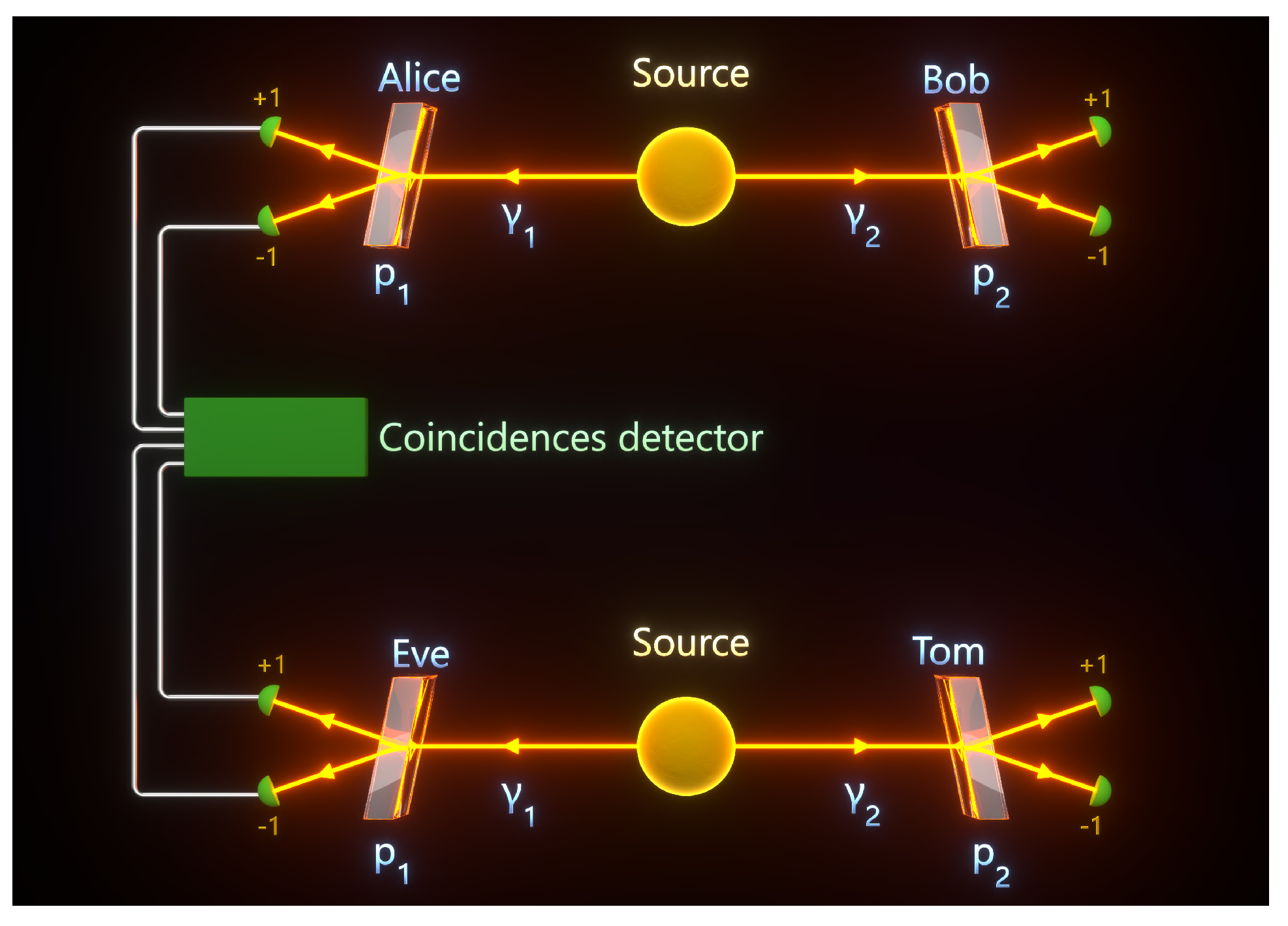
8.1.1. Loophole Controls and Distance-Dependence Test

Of course, to perform a loophole-free test of this kind the polariser settings at each of the four stations must be changed randomly while the photons are in flight between the sources and the polarisers, so that no setting is correlated with the source emission or with the orientations at the other stations, and each measurement event must be spacelike separated from all others, thus closing the locality loophole for the full four-station configuration; the two Bell setups must moreover be suitably electromagnetically shielded in order to avoid any conventional communication channel between them. Beyond these standard precautions, the distance d between Alice and Eve must be varied across experimental runs, since in the present model the bulk-mediated influence between the two pairs depends on d through the factor ${(r_{AB}/r_{AE})}^2$, so that varying d makes it possible to check whether any observed effect follows the expected distance dependence and to rule out spurious correlations as its origin.

A CHSH violation between photons from independent sources is a very demanding experimental test and a negative result would not by itself falsify the theoretical framework proposed in the present work, it could either reflect the practical difficulty of the measurement or the absence of such a strong effect. A clarification is therefore necessary. Each Bell pair should maintain a statistically significant CHSH violation throughout any run, this is not required to define $S_{AE}$, but it excludes trivial explanations of a possible observation of $S_{AE}>2$ due to channel mixing, inadvertent entanglement swapping, or timing artifacts, and reduces the space of conventional alternatives. For this reason, in what follows we also describe a weaker but more accessible test, probing the cross-pair correlation $C\ne 0$ directly without requiring Bell-type violation between non-entangled photons.

8.2. Cross-Pair Correlations: A Weaker but Independent Test

A more accessible experimental target is a nonvanishing cross-pair correlation

$$C=\langle O^{\left(1\right)}{O}^{\left(2\right)}\rangle -\langle O^{\left(1\right)}\rangle \langle O^{\left(2\right)}\rangle ,O^{\left(1\right)}=ij,O^{\left(2\right)}=kl,$$

(170)

between two physically independent entangled photon pairs, where outcome labels take numerical values $\pm \equiv \pm 1$. Standard quantum mechanics predicts $C=0$ by independence of the two sources. In the present framework, a nonzero C can arise if the bulk-mediated contextual input fails to remain separable across the two subsystems.

Consider two sources emitting independent Bell pairs $(A,B)$ and $(E,T)$, corresponding to $(A_1,B_1)$ and $(A_2,B_2)$ in the notation of the preceding section, measured by two distant detector pairs (Alice–Bob and Eve–Tom). The four measurement interactions take place on the brane at laboratory time $t_0$:

$$A=({\mathbf{x}}_A,t_0),B=({\mathbf{x}}_B,t_0),E=({\mathbf{x}}_E,t_0),T=({\mathbf{x}}_T,t_0).$$

(171)

The total Hilbert space factorises at preparation time,

$$\begin{array}{cc}\hfill {\mathcal{H}}_{\mathrm{tot}}& =({\mathcal{H}}_A\otimes {\mathcal{H}}_B)\otimes ({\mathcal{H}}_E\otimes {\mathcal{H}}_T),\hfill \\ \hfill |\Psi (t_0)\rangle & =|{\psi }_{\mathrm{Bell}}^{\left(AB\right)}\rangle \otimes |{\psi }_{\mathrm{Bell}}^{\left(ET\right)}\rangle ,\hfill \end{array}$$

(172)

so standard quantum mechanics predicts statistical independence, $P_{ijkl}=P_{ij}^{\left(AB\right)}{P}_{kl}^{\left(ET\right)}$, and hence $C=0$ identically.

Each measurement interaction activates a localised source term in the bulk equation for ${\mathcal{X}}_a$. With four detector activations the total brane source is ${\sum }_{s\in \{A,B,E,T\}}{J}_a^s\left(x\right)\delta \left(\tau \right)$, and the bulk field obeys

$${\square }_5{\mathcal{X}}_a(x,\tau )=\left[J_a^A\left(x\right)+J_a^B\left(x\right)+J_a^E\left(x\right)+J_a^T\left(x\right)\right]\delta \left(\tau \right).$$

(173)

By linearity, the solution superposes pair contributions at the level of both the bulk field and the brane-evaluated effective contextual signal $\mathcal{Y}$ defined in Eq. (152). Here ${\mathcal{X}}_a^{\left(AB\right)}$ and ${\mathcal{X}}_a^{\left(ET\right)}$ denote the bulk field contributions sourced by the Alice–Bob and Eve–Tom pairs respectively, each satisfying the wave equation (173) with its own pair’s source terms:

$$\begin{array}{cc}\hfill {\mathcal{X}}_a& ={\mathcal{X}}_a^{\left(AB\right)}+{\mathcal{X}}_a^{\left(ET\right)},\hfill \\ \hfill \mathcal{Y}(\mathbf{x},t_0;\lambda )& ={\mathcal{Y}}^{\left(AB\right)}(\mathbf{x},t_0;\lambda )+{\mathcal{Y}}^{\left(ET\right)}(\mathbf{x},t_0;\lambda ).\hfill \end{array}$$

(174)

As established in Secs. Section 5 and Section 4, a localised measurement event sources a bulk field that propagates through the bulk and induces a nonvanishing brane response at all other stations; the field emitted by the Alice–Bob pair reaches the Eve–Tom detector region, and vice versa. For each Bell pair the measurement bases are specified by analyser settings ${\theta }_A,{\theta }_B$ for Alice–Bob and ${\theta }_E,{\theta }_T$ for Eve–Tom, with outcome channels $i,j,k,l\in \{\pm 1\}$, where $(i,j)$ label the Alice–Bob outcomes and $(k,l)$ those of Eve–Tom. The contextual field amplitudes accessible to each detector pair are obtained by projection onto the corresponding outcome modes, in direct analogy with Eq. (155):

$$\begin{array}{cc}\hfill {\mathcal{X}}_{ij}^{\left(AB\right)}(t_0;\lambda )& =\int d^{3}x{u}_{ij}^{\left(AB\right)*}\left(\mathbf{x}\right)\mathcal{Y}(\mathbf{x},t_0;\lambda ),\hfill \end{array}$$

(175)

$$\begin{array}{cc}\hfill {\mathcal{X}}_{kl}^{\left(ET\right)}(t_0;\lambda )& =\int d^{3}x{u}_{kl}^{\left(ET\right)*}\left(\mathbf{x}\right)\mathcal{Y}(\mathbf{x},t_0;\lambda ),\hfill \end{array}$$

(176)

where $u_{ij}^{\left(AB\right)}\left(\mathbf{x}\right)$ and $u_{kl}^{\left(ET\right)}\left(\mathbf{x}\right)$ are the joint two-detector outcome mode functions, defined by

$$\begin{array}{cc}\hfill u_{ij}^{\left(AB\right)}\left(\mathbf{x}\right)& =u_i^{\left(A\right)}\left(\mathbf{x}\right){\mathbf{1}}_{{\Omega }_A}\left(\mathbf{x}\right)+u_j^{\left(B\right)}\left(\mathbf{x}\right){\mathbf{1}}_{{\Omega }_B}\left(\mathbf{x}\right),\hfill \end{array}$$

and analogously for $u_{kl}^{\left(ET\right)}$,with ${\mathbf{1}}_{\Omega }$ the indicator function of the spatial volume $\Omega$ occupied by detector; the single-detector profiles $u_i^{\left(k\right)}\left(\mathbf{x}\right)$ are defined in Eq. (118). The channel-normalised forms are defined by ${\widehat{\mathcal{X}}}_{ij}^{\left(AB\right)}\equiv {\mathcal{X}}_{ij}^{\left(AB\right)}/\left|{\mathcal{X}}^{\left(AB\right)}\right|$ and ${\widehat{\mathcal{X}}}_{kl}^{\left(ET\right)}\equiv {\mathcal{X}}_{kl}^{\left(ET\right)}/\left|{\mathcal{X}}^{\left(ET\right)}\right|$, with $|{\mathcal{X}}^{\left(p\right)}|=(\sum |{\mathcal{X}}_{ij}^{\left(p\right)}{{|}^2)}^{1/2}$, in direct analogy with the single-pair case. Inserting Eq. (174) into (175)–(176) gives

$$\begin{array}{cc}\hfill {\widehat{\mathcal{X}}}_{ij}^{\left(AB\right)}& ={\widehat{\mathcal{X}}}_{ij}^{\left(AB\right)\mathrm{self}}+{\widehat{\mathcal{X}}}_{ij}^{\left(AB\right)\mathrm{cross}},\hfill \end{array}$$

(177)

$$\begin{array}{cc}\hfill {\widehat{\mathcal{X}}}_{kl}^{\left(ET\right)}& ={\widehat{\mathcal{X}}}_{kl}^{\left(ET\right)\mathrm{self}}+{\widehat{\mathcal{X}}}_{kl}^{\left(ET\right)\mathrm{cross}},\hfill \end{array}$$

(178)

where the “self” terms arise from ${\mathcal{Y}}^{\left(AB\right)}$ (resp. ${\mathcal{Y}}^{\left(ET\right)}$) projected at the Alice–Bob (resp. Eve–Tom) stations, and the “cross” terms encode the influence of the opposite Bell setup on the detector-selected contextual readout. The geometric suppression factor ${(r_{AB}/r_{AE})}^2$ of Section 7 controls the relative size of the cross terms: negligible when the two pairs are well separated, growing as Alice and Eve approach each other. As shown in Section 7.4, the relevant criterion for cross-pair independence is not a product decomposition of $\mathcal{Y}$ but separability of the effective four-index contextual input entering Eq. (162). Parametrising the cross contributions by $\epsilon \sim {(r_{AB}/r_{AE})}^2$, which is small when the two pairs are well separated ($r_{AE}\gg r_{AB}$), the minimal nonseparable ansatz is

$${\tilde{R}}_{ijkl}(t_0;\lambda )={\tilde{R}}_{ij}^{\left(AB\right)}(t_0;{\lambda }_1)+{\tilde{R}}_{kl}^{\left(ET\right)}(t_0;{\lambda }_2)+\epsilon {\Delta }_{ijkl}^{\left(R\right)}(t_0;\lambda ),$$

(179)

where ${\Delta }_{ijkl}^{\left(R\right)}$ is a cross-indexed contribution that cannot be absorbed into a function of $(i,j)$ plus a function of $(k,l)$. It arises because ${\mathcal{X}}_a$ projects onto both detector regions simultaneously via the cross terms in (177)–(178), so that the contextual microstate $\lambda$ contains components influencing the readouts of both pairs; ${\Delta }_{ijkl}^{\left(R\right)}$ quantifies this mutual influence. Its explicit form depends on the preparation source $J_a$ and the detector geometry; establishing it requires a microscopic model of $J_a^{\left(\mathrm{prep}\right)}$ that lies beyond the scope of the present work, and is unnecessary for the order-of-magnitude prediction of C derived below.

For a fixed contextual microstate $\lambda$, the collapse dynamics is deterministic and the nonlinear evolution (162) drives the amplitudes to a definite outcome $(i,j,k,l)$ once the collapse dynamics has run to completion, i.e. at times sufficiently later than the measurement onset $t_0$. If the contextual input is separable ($\epsilon =0$), the two-pair dynamics preserves effective independence and $P_{ijkl}=P_{ij}^{\left(AB\right)}{P}_{kl}^{\left(ET\right)}$, hence $C=0$. With the nonseparable term present, the ensemble distribution takes the form

$$P_{ijkl}=P_{ij}^{\left(AB\right)}{P}_{kl}^{\left(ET\right)}+\epsilon \delta P_{ijkl},$$

(180)

where $\delta P_{ijkl}$ is constrained by normalisation and no-signaling but need not vanish, and where the zeroth-order term factorises exactly by the equivariance condition of Section 6.4, ensuring $C_0=0$ precisely. Defining the induced marginal corrections

$$\delta P_{ij}^{\left(AB\right)}\equiv \sum _{k,l=\pm 1}\delta P_{ijkl},\delta P_{kl}^{\left(ET\right)}\equiv \sum _{i,j=\pm 1}\delta P_{ijkl},$$

(181)

the cross-correlation to leading order in $\epsilon$ reads

$$\begin{array}{ccc}\hfill C& =& \epsilon [\underset{\mathrm{joint}\mathrm{correction}}{\underbrace{{\sum }_{i,j,k,l=\pm 1}\left(ij\right)\left(kl\right)\delta P_{ijkl}}}\hfill \\ & -& \underset{\mathrm{shift}\mathrm{in}\langle O^{\left(1\right)}\rangle \mathrm{from}\delta P}{\underbrace{\left({\sum }_{i,j=\pm 1}\left(ij\right)\delta P_{ij}^{\left(AB\right)}\right)\left({\sum }_{k,l=\pm 1}\left(kl\right)P_{kl}^{\left(ET\right)}\right)}}\hfill \\ & -& \underset{\mathrm{shift}\mathrm{in}\langle O^{\left(2\right)}\rangle \mathrm{from}\delta P}{\underbrace{\left({\sum }_{i,j=\pm 1}\left(ij\right)P_{ij}^{\left(AB\right)}\right)\left({\sum }_{k,l=\pm 1}\left(kl\right)\delta P_{kl}^{\left(ET\right)}\right)}}]+\mathcal{O}\left({\epsilon }^2\right).\hfill \end{array}$$

The three bracketed terms represent, respectively, the leading joint-outcome correction and the shifts in $\langle O^{\left(1\right)}\rangle$ and $\langle O^{\left(2\right)}\rangle$ induced by $\delta P$. Whenever ${\Delta }_{ijkl}^{\left(R\right)}$ generates a joint-outcome correction that is not accounted for by these single-pair mean shifts alone, C is nonzero at order $\epsilon$.

Quantitative estimate of $C_{AE}$ and event requirements.

The cross-pair correlator arises from the cross-pair zero-mode pulse contributions to the full four-index contextual drive ${\tilde{R}}_{ijkl}$, and, as established above (Eq. (164)), the nonseparable term ${\Delta }_{ijkl}$ scales as ${(r_{AB}/r_{AE})}^2$, which enters the $\epsilon$-expansion of Eq. (182) to give $C_{AE}\sim \epsilon$. With the identification $r_{AB}\sim \mathsf{\ell }$ (intra-pair baseline) and $r_{AE}\sim d$ (inter-source distance), one therefore obtains

$$\epsilon \sim {\left({\displaystyle \frac{\mathsf{\ell }}{d}}\right)}^2,C_{AE}\sim \epsilon \sim {\left({\displaystyle \frac{\mathsf{\ell }}{d}}\right)}^2,$$

(182)

in the zero-mode dominated regime. Notice that since both $|{\psi }_i^{\left(k\right)}{|}^2$ and $|{\widehat{\mathcal{X}}}_i^{\left(k\right)}{|}^2$ are normalised quantities, the overall amplitude of ${\mathcal{X}}_a$ cancels in the ratio (155), and therefore the prediction is independent of the absolute normalisation of ${\mathcal{X}}_a$. If the relevant modes are instead massive (KK sector), the Yukawa form of the Green function gives

$$C_{AE}\sim {\left({\displaystyle \frac{\mathsf{\ell }}{d}}\right)}^2{e}^{-\mu d},$$

(183)

that is, exponentially suppressed for $d\gg {\xi }_{\mathrm{KK}}$, so that varying d at fixed ℓ distinguishes the two regimes: a power-law decay signals the zero-mode channel while an exponential decay signals a massive spectrum.

Event requirements. Resolving $C_{AE}\sim {(\mathsf{\ell }/d)}^2$ above statistical noise requires $N\sim {(d/\mathsf{\ell })}^4$ coincidence events per setting combination; three representative configurations are listed in the table below.

ℓ	d	$C_{AE}\sim {(\mathsf{\ell }/d)}^2$	$N\sim {(d/\mathsf{\ell })}^4$	setup
1 m	10 m	${10}^{-2}$	${10}^4$	tabletop
1 m	30 m	${10}^{-3}$	${10}^6$	extended lab
1 m	100 m	${10}^{-4}$	${10}^8$	demanding

The tabletop configuration ($\mathsf{\ell }=1$ m, $d=10$ m) is the most accessible, with $C_{AE}\sim {10}^{-2}$ and $N\sim {10}^4$ events per setting combination, both within reach of existing photonic Bell experiments [2,3,4,14], while the demanding configuration ($\mathsf{\ell }=1$ m, $d=100$ m) illustrates the steep ${(d/\mathsf{\ell })}^4$ scaling of event requirements at larger separations.

Spectral structure, the role of k, and experimental implications.

Two spectral channels. The $\tau$-spectrum of ${\mathcal{X}}_a$ splits into a normalizable zero mode with ${\mu }_0=0$ and a continuum of massive modes $\mu \in (0,\infty )$ (Section 3.3.2; see also [33,38]). The zero mode carries brane overlap ${\psi }_0\left(0\right)=\sqrt{k}\ne 0$ and mediates a massless four-dimensional field; its equal-time two-point function,

$$C^{\left(0\right)}(0,r)={\displaystyle \frac{1}{4{\pi }^2{r}^2}},$$

(184)

is a pure power law holding for $r\gg {\xi }_{\mathrm{KK}}\equiv w/k$. The continuum contributes Yukawa-suppressed two-point functions

$$C^{\left(\mu \right)}\left(r\right)\sim \varrho \left(\mu \right){\displaystyle \frac{e^{-\mu r}}{r}},$$

(185)

which only become comparable to the zero-mode term at $r\lesssim {\xi }_{\mathrm{KK}}$; beyond that scale the massive sector is simply irrelevant. There is no discrete KK tower, since a discrete spectrum would require compactification or a confining mechanism in $\tau$, and neither is present.

The role of k and observational bound. The warping parameter k drops out of the power-law falloff (184) entirely; its only footprint in observable predictions is the crossover scale ${\xi }_{\mathrm{KK}}=w/k$. The lower bound $k\gtrsim 3\times {10}^{11}$ ${\mathrm{s}}^{-1}$ comes from spooky-action speed experiments [12,13], and with the natural choice $w=c$ the zero mode dominates on every laboratory scale of interest.

Predicted signal as a function of separation. For given ℓ, the cross-pair correlation reads

$$C_{AE}\left(d\right)\sim \underset{\begin{array}{c}\mathrm{zero}\mathrm{mode}\\ (\mathrm{prep}.)\end{array}}{\underbrace{{\left({\displaystyle \frac{\mathsf{\ell }}{d}}\right)}^2}}+\underset{\begin{array}{c}\mathrm{KK}\sec \mathrm{tor}\\ (\mathrm{prep}.)\end{array}}{\underbrace{{\left({\displaystyle \frac{\mathsf{\ell }}{d}}\right)}^2{e}^{-d/{\xi }_{\mathrm{KK}}}}}+\underset{\begin{array}{c}\mathrm{exchange}\\ (\mathrm{meas}.)\end{array}}{\underbrace{C_{\mathrm{exch}}{e}^{-d^2/2d_{\mathrm{exch}}^2}}},$$

(186)

valid for $d\gg \mathsf{\ell }$. The first two terms come from the preparation-encoded non-factorising field configuration (Section 6.5); the third from the measurement-exchange mechanism (Section 6.3, assumptions H1–H3), with crossover scale $d_{\mathrm{exch}}=w\delta \tau$ and $O\left(1\right)$ coefficient $C_{\mathrm{exch}}$ left free. At large d the Gaussian dies first, then the KK Yukawa; what survives at long range is the zero-mode power law alone. Standard quantum mechanics gives $C_{AE}=0$ at every d.

Main experimental prediction. The cross-pair correlation indicator

$$C_{AE}\sim {\left({\displaystyle \frac{\mathsf{\ell }}{d}}\right)}^2$$

(187)

is the central falsifiable prediction of this work. Standard quantum mechanics gives $C_{AE}=0$ always; here $C_{AE}\ne 0$ with a value fixed by $\mathsf{\ell }/d$ alone, no free amplitude enters the leading term. The protocol demands no CHSH violation between non-entangled photons and is within reach of current photonic Bell technology: two independent SPDC sources at variable separation d, run along the lines of Refs. [2,3,4,14], would be enough.

Experimental protocol. The core protocol consists of varying d at fixed ℓ and recording $C_{AE}\left(d\right)$. Alice and Eve each receive one photon from their respective source, and Bob and Tom receive the partner photons. At each separation d, coincidence statistics must be accumulated sufficient to resolve $C_{AE}$, that is, $N\sim {(d/\mathsf{\ell })}^4$ events per setting combination (see table above). As required by the consistency check of Section 8.1.1, Bob and Tom must maintain a statistically significant CHSH violation with their respective partners throughout every run, thus confirming that the AB and ET pairs remain entangled and ruling out conventional cross-talk as the origin of any observed $C_{AE}\ne 0$. The predicted curve (186) exhibits three separable regimes, each constraining a different physical parameter: a Gaussian decay constrains ${\mathsf{\ell }}_{\mathrm{exch}}=w\delta \tau$ and hence the detector $\tau$-thickness $\delta \tau$; a power-law decay ${(\mathsf{\ell }/d)}^2$ at intermediate d identifies the zero-mode channel; and a downward deviation from the power law at large d constrains ${\xi }_{\mathrm{KK}}=w/k$ and hence the warping parameter k. These regimes are well separated provided ${\mathsf{\ell }}_{\mathrm{exch}}\ll {\xi }_{\mathrm{KK}}\ll d_{\max }$, where $d_{\max }$ is the maximum experimental baseline, and with ${\xi }_{\mathrm{KK}}=c/k\sim 1$ mm for $k\sim 3\times {10}^{11}$ ${\mathrm{s}}^{-1}$ this condition is met for any laboratory-scale $d_{\max }$.

Summary of Section 8. Two experimental tests are proposed. The strong test (Section 8.1) looks for a CHSH violation $S_{AE}>2$ between photons from independent sources; a positive result would be unambiguous but the test is experimentally demanding. The weaker test (Section 8.2) looks instead for $C_{AE}\ne 0$ and its d-dependence, requires no Bell violation between non-entangled photons, and is accessible with existing photonic Bell technology [2,3,4,14]. Any nonzero $C_{AE}$ displaying this d-dependence is at odds with standard quantum mechanics; this test is logically independent of Bell–CHSH constraints and experimentally less demanding than the strong test of Section 8.1. The predicted scaling $C_{AE}\sim {(\mathsf{\ell }/d)}^2$, a direct consequence of zero-mode dominance in the warped $(3,2)$ geometry, has no counterpart in standard quantum mechanics, and varying d at fixed ℓ is the natural experimental handle to test it.

9. Discussion and Concluding Remarks

The present work shows that, within a warped $(3,2)$ spacetime, the bulk propagation of a field ${\mathcal{X}}_a$ projects onto the $(3,1)$ brane producing equal-time correlations at arbitrary separation, and this occurs without controllable superluminal signalling on the brane. The mechanism is geometric: it does not depend on the details of the collapse realisation, and the experimental signature derived here, a cross-pair correlator $C_{AE}\sim {(\mathsf{\ell }/d)}^2$ in the zero-mode-dominated regime, with the predicted functional form given in Eq. (186), is a joint consequence of that geometry and the Bohm–Bub collapse dynamics coupled to it.

The warp function $f\left(\tau \right)=k\left|\tau \right|$ entering the $(3,2)$ spacetime metric is the unique solution, up to sign and an additive constant, of the vacuum Einstein equations compatible with ${\mathbb{Z}}_2$ symmetry; it is not a modelling choice. Within this geometric setting, the $E=0$ null geodesic family connects brane points at equal coordinate time regardless of their spatial separation, allowing equal-time correlations at arbitrary distance without any further assumption. That a warped $(4,1)$ spacetime admits no analogous shortcut rules out extra spatial dimensions as mediators; the extra dimension must be temporal. A t-retarded prescription preserves causality and no-signaling at the level of brane observables.

Coupling the bulk field ${\mathcal{X}}_a$ to the collapse dynamics, Born statistics follow whenever $\rho \left(\lambda \right)$ is equivariant, and standard quantum-mechanical predictions are recovered in all single-pair configurations. The only departure is in the cross-pair correlator: $C_{AE}\ne 0$ with $C_{AE}\sim {(\mathsf{\ell }/d)}^2$, conditional on assumptions (H1)–(H3) of Section 6.3. This scaling follows from the zero-mode amplitude ratio and is insensitive to the specific form of the collapse equation or the readout map; it is a robust geometric prediction, not an artefact of the particular collapse realisation chosen. The signal has no counterpart in standard quantum mechanics. Varying d at fixed ℓ is the natural experimental handle, a test that would be dismissed as trivial in the absence of the physical hypothesis put forward here, but whose outcome is genuinely informative once that hypothesis is stated precisely enough to be falsified.

9.1. What Is Proved, What Is Assumed, and What Remains Open

Metric ansatz and GR consistency.

We have shown that the warped $(3,2)$ metric ansatz with $f\left(\tau \right)=k\left|\tau \right|$ satisfies the five-dimensional vacuum Einstein equations with positive bulk cosmological constant; the bulk Einstein equations projected onto the $\tau =0$ brane then take the Randall–Sundrum form with $E_{\mu \nu }=0$ at leading order, so that the standard four-dimensional gravitational physics is recovered on the brane without any fine-tuning beyond the ansatz itself. See Section 3.2 and Appendix A.

Brane-to-brane retarded Green function.

For each effective four-dimensional mode of $({\square }_4+{\mu }^2)$, the retarded Green function is standard and well posed [25,40]; the retarded brane-time prescription eliminates the operational ultrahyperbolic pathology by reducing each mode to a well-posed four-dimensional Cauchy problem, so that the ultrahyperbolic character of the full $(3,2)$ wave operator is, in fact, harmless at the level of brane observables. What remains assumed is that the resulting sum over admissible components converges in the distributional sense, by analogy with the mode-sum convergence established for the Randall–Sundrum graviton propagator [38]; a fully rigorous proof is deferred to future work.

Equal-time reach.

The $E=0$ null geodesic family consists of curves with $\dot{t}\equiv 0$, connecting brane points at equal brane time and at arbitrarily large separation; see Section 4. In the WKB representation of the brane-to-brane kernel this family appears as the stationary-phase saddle ${\partial }_{t}S=0$, giving the leading contribution to equal-time correlations at large separation, in other words, equal-time brane correlations are not exponentially suppressed at large r, and this is a direct structural consequence of the warped metric, not an additional assumption.

No-signaling.

In the linear sector, the retarded support of $G_{\mathrm{ret}}$ ensures that the field response to any brane source is strictly light-cone limited; see Section 5.4. In the nonlinear Bohm–Bub collapse sector, physically relevant single-party probabilities arise only after averaging over $\rho \left(\lambda \right)$; when $\rho \left(\lambda \right)$ is equivariant those marginals coincide with the standard quantum-mechanical ones and remain setting independent, so that no-signaling is recovered there as well, without any further assumption beyond equivariance itself.

Born rule.

Born statistics are recovered under the assumption that $\rho \left(\lambda \right)$ is equivariant; see Appendix B and Secs. Section 6 and Section 7. What remains open is whether generic initial distributions relax dynamically toward that class; establishing an analogue of the Bohmian subquantum H-theorem [57] for the present contextual collapse dynamics is still to be done, and equivariance of $\rho \left(\lambda \right)$ should therefore be regarded as a consistency condition of the present implementation rather than as a theorem derived from the dynamics.

Detector-map robustness.

The map ${\mathcal{F}}_{ij}$ is not uniquely determined by locality and measurement-basis symmetries, although those requirements delimit the admissible class. Within that class the scaling $C_{AE}\sim {(\mathsf{\ell }/d)}^2$ and its dependence on d are insensitive to the particular choice of ${\mathcal{F}}_{ij}$: the ${(\mathsf{\ell }/d)}^2$ factor stems from the ratio of zero-mode amplitudes at the intra-pair separation ℓ and the inter-pair separation d, in which all map-dependent prefactors cancel exactly.

Preparation-dominance condition.

The assumption that the preparation field dominates the denominator of ${\tilde{R}}_j^{\left(B\right)}$ (Eq. (139)) is not a consequence of the bulk wave equation; it requires that the preparation source generate a substantially stronger bulk excitation than a single detector-induced measurement pulse, and its fulfilment is deferred to the microscopic model of $J_a^{\left(\mathrm{prep}\right)}$. When this condition holds, equivariance and Born-rule recovery are unmodified, and the exchange term enters as a controlled perturbation.

Encoding of specific quantum correlations in the bulk field.

What is established is that ${\mathcal{X}}_a$ does not factorise: the bulk field sourced at $x_{\mathrm{prep}}$ reaches the brane in a configuration that admits no decomposition into independent contributions at $x_A$ and $x_B$, this is, precisely, the field-theoretic analogue of entanglement. What is not yet derived from the bulk dynamics alone is the detailed correlation structure of the prepared state, including singlet anticorrelation, the precise angular dependence of the two-detector correlator on the analyser settings, and the Tsirelson bound, since in the present formulation that structure is encoded in the single-station projection maps, which are constrained by equivariance but not uniquely fixed by it. A natural ansatz for $J_a^{\left(\mathrm{prep}\right)}$ compatible with singlet structure is given in Section 6.5 [Eqs. (129)–(128)], and the central open task is to verify that this ansatz yields a brane field satisfying condition (130). Two issues therefore remain open: contextual equilibration and the derivation of the readout maps from the preparation source, the second being the deeper one, because resolving it would make the observed quantum correlation structure emerge from the geometry rather than be inserted as compatible input. This derivation will be taken up in a companion paper.

Detector assumptions (H1)–(H3).

Assumptions (H1)–(H3) of Section 6.3 are modelling inputs of the Bohm–Bub-based realisation, not consequences of the geometry itself: (H1) relaxes strict brane confinement by postulating a finite $\tau$-profile for detectors; (H2) promotes measurement interactions to bulk sources away from $\tau =0$; and (H3) assumes that the measurement-sourced pulse carries outcome information but not setting information. These assumptions are physically motivated and mutually consistent, but they are not yet derived from a microscopic model of the detector. The signature $C_{AE}\sim {(\mathsf{\ell }/d)}^2$ is therefore a prediction of the geometry together with this class of collapse realisations; any model that couples a local contextual input to the bulk field${\mathcal{X}}_a$ inherits the same geometric scaling, since the ${(\mathsf{\ell }/d)}^2$ factor follows from the zero-mode amplitude ratio and is independent of the specific nonlinear form of the collapse equation.

To conclude, entanglement defies our usual representations and understanding of physical phenomena; this is not because quantum mechanics is wrong, but because the causal structure it requires appears inexplicable within our $(3,1)$ dimensional spacetime. The construction proposed in the present work offers one possible way to extend this spacetime structure while retaining compatibility with known constraints, and makes a specific, geometry-dependent experimental prediction that is testable with existing photonic Bell technology.

Appendix A.1. Induced Geometry and Extrinsic Curvature

Let $x^{\mu }$ ($\mu =0,1,2,3$) be intrinsic coordinates on the brane and $X^A\left(x^{\mu }\right)$ the embedding map. The tangent basis is

$${e^A}_{\mu }\equiv {\displaystyle \frac{\partial X^A}{\partial x^{\mu }}},n_A{e^A}_{\mu }=0.$$

(A3)

The projector onto directions tangent to the brane is

$$h_{AB}\equiv g_{AB}^{\left(5\right)}-ϵn_A{n}_B,$$

(A4)

and the induced metric is the pullback

$$g_{\mu \nu }^{\left(4\right)}=h_{AB}{e^A}_{\mu }{e^B}_{\nu }=g_{AB}^{\left(5\right)}{e^A}_{\mu }{e^B}_{\nu }.$$

(A5)

The extrinsic curvature,

$$K_{\mu \nu }\equiv {e^A}_{\mu }{e^B}_{\nu }{\nabla }_A{n}_B,$$

(A6)

measures how the brane is curved within the bulk (it vanishes if the brane is totally geodesic). We denote $K\equiv {K^{\alpha }}_{\alpha }$.

Appendix A.2. Gauss–Codazzi Projection and Effective Brane Equation

Projecting the bulk curvature via the Gauss equation and contracting yields an effective four-dimensional Einstein equation of the schematic form

$$G_{\mu \nu }^{\left(4\right)}={\mathcal{S}}_{\mu \nu }+Q_{\mu \nu }-ϵE_{\mu \nu },$$

(A7)

where:

(i) ${\mathcal{S}}_{\mu \nu }$ collects the direct contribution of the bulk field equations (A1). For a pure bulk cosmological constant, ${\mathcal{S}}_{\mu \nu }$ is proportional to $g_{\mu \nu }^{\left(4\right)}$ and is conveniently absorbed into an effective brane cosmological constant once the junction conditions are imposed (see below).

(ii) $Q_{\mu \nu }$ is the local correction quadratic in the extrinsic curvature,

$$\begin{array}{ccc}\hfill Q_{\mu \nu }& =& ϵ\left[K{K}_{\mu \nu }-K_{\mu \alpha }{K^{\alpha }}_{\nu }-{\displaystyle \frac{1}{2}}{g}_{\mu \nu }^{\left(4\right)}\left(K^2-K_{\alpha \beta }{K}^{\alpha \beta }\right)\right].\hfill \end{array}$$

The explicit factor $ϵ\equiv n_A{n}^A$ keeps track of whether the normal is spacelike ($ϵ=+1$) or timelike ($ϵ=-1$), and therefore reverses the overall sign of $Q_{\mu \nu }$ when passing between the two cases.

(iii) $E_{\mu \nu }$ is the nonlocal Weyl projection,

$$E_{\mu \nu }\equiv C_{ABCD}^{\left(5\right)}{n}^A{e^B}_{\mu }{n}^C{e^D}_{\nu },$$

(A8)

which encodes bulk gravitational degrees of freedom not fixed by local brane data. It is traceless, ${E^{\mu }}_{\mu }=0$, and (in the absence of bulk matter) its divergence is constrained by the projected Bianchi identities (see Refs. [60,61]).

With these definitions, the effective brane equation involves the combination $-ϵE_{\mu \nu }$. Thus for a timelike extra dimension ($ϵ=-1$) the Weyl projection enters as $+E_{\mu \nu }$, whereas for a spacelike extra dimension ($ϵ=+1$) it enters with the opposite sign; the same $ϵ$ factor also fixes the overall sign of the local quadratic term $Q_{\mu \nu }$.

Appendix A.3. Israel Junction Condition, Z 2 Symmetry, and Vacuum Brane

Let $S_{\mu \nu }$ be the brane stress tensor (including tension). In the present sign convention, a compact $ϵ$-explicit form of the Israel junction condition is

$$ϵ\left(\left[K_{\mu \nu }\right]-g_{\mu \nu }^{\left(4\right)}\left[K\right]\right)=-{\kappa }_5^2{S}_{\mu \nu },$$

(A9)

where $\left[K_{\mu \nu }\right]$ denotes the jump of $K_{\mu \nu }$ across the brane. Equivalently (solving (A9) for $\left[K_{\mu \nu }\right]$),

$$\left[K_{\mu \nu }\right]=-ϵ{\kappa }_5^2\left(S_{\mu \nu }-{\displaystyle \frac{1}{3}}{g}_{\mu \nu }^{\left(4\right)}S\right),S\equiv g^{\left(4\right)\mu \nu }{S}_{\mu \nu },$$

(A10)

which is the form used below. With ${\mathbb{Z}}_2$ symmetry (mirror symmetry across the brane), one has $K_{\mu \nu }^{+}=-K_{\mu \nu }^{-}$ and hence $\left[K_{\mu \nu }\right]=2K_{\mu \nu }^{+}$, so (A10) fixes $K_{\mu \nu }$ algebraically in terms of $S_{\mu \nu }$ once an orientation for $n^A$ is chosen.

For a vacuum brane with pure tension,

$$S_{\mu \nu }=-\sigma g_{\mu \nu }^{\left(4\right)},$$

(A11)

the junction condition implies $K_{\mu \nu }\propto g_{\mu \nu }^{\left(4\right)}$ and the local term $Q_{\mu \nu }$ reduces to an effective cosmological-constant contribution. One may then write the induced brane equation in the compact form

$$G_{\mu \nu }^{\left(4\right)}+{\Lambda }_4{g}_{\mu \nu }^{\left(4\right)}=-ϵE_{\mu \nu },$$

(A12)

with

$${\Lambda }_4={\displaystyle \frac{1}{2}}{\kappa }_5^2\left({\Lambda }_5+ϵ{\displaystyle \frac{{\kappa }_5^2{\sigma }^2}{6}}\right).$$

(A13)

in direct analogy with the usual brane-world relation, now keeping explicit the sign $ϵ=-1$ appropriate to a timelike extra dimension.

The constants ${\kappa }_5$, ${\Lambda }_5$, $\sigma$, and k are not all independent. The parameter k is the same inverse curvature scale that appears in the warp factor $f\left(\tau \right)=k\left|\tau \right|$; it has dimensions of inverse time ($k\sim c/L_{\mathrm{bulk}}$ where $L_{\mathrm{bulk}}$ is the bulk curvature length scale) and is the single bulk scale of the construction. The bulk cosmological constant is related to k and the five-dimensional gravitational coupling ${\kappa }_5^2=8\pi G_5$ by the $\left(\tau \tau \right)$ component of the bulk Einstein equations, which for $ϵ=-1$ yields ${\Lambda }_5=+6k^2/{\kappa }_5^2$, requiring ${\Lambda }_5>0$, i.e. a de Sitter-type bulk. This is the correct sign for a timelike extra dimension: unlike the standard Randall–Sundrum case ($ϵ=+1$), where the $\left(\tau \tau \right)$ equation gives ${\Lambda }_5^{\mathrm{RS}}=-6k^2/{\kappa }_5^2<0$ (AdS), the sign flip in $g_{\tau \tau }=-w^2$ reverses the equation and requires a positive bulk cosmological constant (see also the remark in Section 3.2). The brane tension $\sigma$ satisfies the fine-tuning condition $\sigma =6k/{\kappa }_5^2$, which entails ${\Lambda }_4=0$, as verified by substituting into (A13) with $ϵ=-1$:

$${\Lambda }_4=\frac{1}{2}{\kappa }_5^2\left({\displaystyle \frac{6k^2}{{\kappa }_5^2}}-{\displaystyle \frac{{\kappa }_5^2}{6}}·{\displaystyle \frac{36k^2}{{\kappa }_5^4}}\right)=\frac{1}{2}{\kappa }_5^2·{\displaystyle \frac{6k^2}{{\kappa }_5^2}}\left(1-1\right)=0.$$

(A14)

This is the analogue of the Randall–Sundrum tuning condition [32,33] applied to the case with $ϵ=-1$. This condition is adopted here for definiteness and is not essential to the construction; a small nonzero ${\Lambda }_4$ consistent with the observed cosmological constant could be accommodated by a slight detuning of the brane tension via (A13), without affecting the bulk-mediated correlation mechanism at the scales relevant to the present work. The effective four-dimensional Newton constant is $G_4=G_{5}k/\left(4\pi c\right)$, which imposes one relation between the two bulk parameters ${\kappa }_5$ and k, leaving one of them free once $G_4$ is fixed to its measured value. The factor of c is required by dimensional consistency: in the present $(3,2)$ framework $\left[k\right]={\mathrm{s}}^{-1}$, so the standard RS relation $G_4=G_5{k}_{\mathrm{RS}}/\left(4\pi \right)$ (with $\left[k_{\mathrm{RS}}\right]={\mathrm{m}}^{-1}$) must be replaced by $G_4=G_5(k/c)/\left(4\pi \right)$.

In the ${\mathbb{Z}}_2$-symmetric thin brane background with $f\left(\tau \right)=k\left|\tau \right|$ considered in Section 3.2, the bulk is piecewise of constant curvature, so $C_{ABCD}^{\left(5\right)}=0$ away from $\tau =0$ and $E_{\mu \nu }=0$ on the brane. The non-smoothness of the metric at $\tau =0$ produces a delta-function contribution to the Ricci tensor localised on the brane, but no analogous singular term appears in the Weyl tensor. The tensor $E_{\mu \nu }$, the projection of the bulk Weyl tensor onto the brane, which encodes the influence of the bulk geometry on four-dimensional gravity [60], vanishes identically on the unperturbed background because the bulk is conformally flat. It becomes nonzero only in the presence of bulk perturbations, and its magnitude is then controlled by the ratio of the perturbation amplitude to the bulk curvature scale k. When the RS-type approximation is valid, this ratio is small by assumption, so $E_{\mu \nu }$ enters as a small, controlled correction rather than a leading-order effect.

As analysed for broad classes of backgrounds in Ref. [62], extra dimensions with timelike signature can in general support ghost-like instabilities or runaway modes, because the wrong-sign kinetic term associated with a timelike direction allows perturbations to grow without bound. Whether the present background is perturbatively stable has not been established by a complete linear perturbation analysis; the following is therefore a plausible argument, not a proved result.

Two structural features suggest that the present construction avoids the most dangerous instability channels. First, the ${\mathbb{Z}}_2$ symmetry restricts the physical spectrum to modes even under $\tau \to -\tau$, which removes the odd-parity sector where ghost modes generically appear in timelike extra-dimension constructions. Second, the positive bulk cosmological constant makes the bulk geometry de Sitter-like in the $\tau$-direction, providing a curvature contribution that can stabilise the vacuum against small perturbations. Whether these two conditions are jointly sufficient to render the background perturbatively stable requires a dedicated Hamiltonian or mode-energy analysis that goes beyond the scope of this work, and is left as an open problem.

Appendix B.1. Contextual Variable λ as a Coarse-Graining of Bulk Microstructure

Within any single run, once $\lambda$ is assigned, collapse is deterministic. The complete bulk microstate, the field configuration ${\mathcal{X}}_a(x,\tau )$ at every point in the five-dimensional bulk, is, strictly speaking, an infinite-dimensional object, neither directly accessible to observation nor tractable as a whole. In practice, what governs collapse is far less: a single effective contextual coordinate,

$$\lambda \equiv \lambda \left[{\mathcal{X}}_a\right],$$

(A15)

a functional that compresses the full bulk field into the single label on which the deterministic collapse outcome depends. Many distinct bulk configurations project onto the same $\lambda$; distinct collapse outcomes arise only when $\lambda$ differs.

Appendix B.2. Run-to-Run Fluctuations and Born Statistics

Microscopic variations in the brane source $J_a$, environmental noise, and the unavoidable imperfections of any real apparatus cause $\lambda$ to fluctuate from run to run. Within each run, conditionally on $\lambda$, the Bohm–Bub dynamics is fully deterministic; the statistical character of quantum mechanics enters only through the averaging,

$$P_i={\int }_{{\Lambda }_i}\rho \left(\lambda \right)d\lambda ,$$

(A16)

where ${\Lambda }_i$ is the basin of attraction for outcome i. The question, then, is: which $\rho \left(\lambda \right)$ reproduces the Born rule $P_i={\left|{\psi }_i\right|}^2$?

In Bohmian mechanics the answer has been known for some time: quantum equilibrium [57], the condition that $\rho \left(q\right)={|\Psi \left(q\right)|}^2$ be preserved by the guidance equation, is sufficient to recover the Born rule from within the dynamics rather than by postulate. Tutsch [46] showed that something analogous holds for the original Bohm–Bub model, an equivariance condition on $\rho \left(\lambda \right)$ with respect to the nonlinear collapse flow is sufficient to preserve Born weights in time. We follow the same route.

Appendix Equivariance under the BB collapse flow.

The BB-type evolution (124) drives an initial amplitude vector $\psi \left(t_0\right)$ into channel $i^{*}$ on a timescale $\sim {\gamma }^{-1}$; the basin ${\Lambda }_i$ is simply the set of all contextual points that end up at outcome i. For the Born rule to hold and remain stable under repeated measurements, $\rho \left(\lambda \right)$ must satisfy, for every measurement basis and every outcome i,

$${\int }_{{\Lambda }_i}\rho \left(\lambda \right)d\lambda ={\left|{\psi }_i\left(t_0\right)\right|}^2.$$

(A17)

This is, in the end, a consistency requirement rather than a derivation: it demands that the ensemble distribution over contextual microstates be compatible with the quantum state, in exactly the same sense that $\rho \left(q\right)={|\Psi \left(q\right)|}^2$ is compatible with the Bohmian velocity field. A distribution satisfying (A17) for all bases will be called equivariant for the contextual collapse dynamics. Whether a generic initial distribution actually relaxes toward such a form is a deeper question altogether, one that would require something like a sub-quantum H-theorem, which we do not attempt here. The goal of the next subsection is more modest: to show that equivariant distributions are not empty as a class, and in fact admit a natural explicit construction.

Appendix B.3. A Concrete Equivariant Family: Drift-Diffusion with Logarithmic Potential

Within each run, the Bohm–Bub dynamics drives $\lambda$ deterministically toward one of the collapse attractors ${\lambda }_i$. Across runs, however, its initial value is effectively random, set, in each experimental realisation, by whatever microscopic fluctuations happened to be present in $J_a$, in the environment, and in the apparatus at that moment. It is $\lambda$ itself, understood as a coarse-graining of the full bulk microstructure, that wanders through the space of possible field configurations from one run to the next. The simplest framework consistent with this picture is a drift-diffusion process in which a deterministic drift toward the attractors competes with diffusion originating from the run-to-run randomness of the initial preparation. It should be said clearly that this is a modelling assumption, not a derivation: there is nothing in the microscopic dynamics of ${\mathcal{X}}_a$ that forces the coarse-grained evolution of $\lambda$ to be either Markovian or diffusive, and a more fundamental treatment of this question remains open, at roughly the same level of difficulty as the sub-quantum H-theorem invoked above. The Fokker–Planck framework is adopted here simply because it is tractable and, as will be seen, yields an explicit equivariant stationary distribution.

If the effective evolution of $\lambda$ is Markovian at the coarse-grained level, $\rho (\lambda ,t)$ obeys a Fokker–Planck equation,

$${\displaystyle \frac{\partial \rho }{\partial t}}=-{\displaystyle \frac{\partial }{\partial \lambda }}\left[F\left(\lambda \right)\rho \right]+D{\displaystyle \frac{{\partial }^2\rho }{\partial {\lambda }^2}},D>0,$$

(A18)

where $F\left(\lambda \right)=-dU/d\lambda$ is a drift force derived from a potential $U\left(\lambda \right)$, and D parametrizes the strength of contextual diffusion. Stationary solutions with vanishing probability current are [63]

$${\rho }_{\mathrm{stat}}\left(\lambda \right)\propto e^{-U\left(\lambda \right)/D}.$$

(A19)

For ${\rho }_{\mathrm{stat}}$ to satisfy the equivariance condition (A17), the weight must pile up near each attractor ${\lambda }_i$ in proportion to $|{\psi }_i{|}^2$. Two conditions govern how this concentration must work: basin weights must be independent of where exactly the basin boundaries fall, and no parameter beyond ${\alpha }_i$ may characterise the focusing near ${\lambda }_i$.

Near ${\lambda }_i$ the distribution must accordingly be singular, a non-singular distribution would make the basin weight depend on the precise location of the boundary, in violation of the first condition. The second condition then forces the singularity into the unique power-law form ${\rho }_{\mathrm{stat}}\sim {|\lambda -{\lambda }_i|}^{-{\alpha }_i}$, with $0<{\alpha }_i<1$ for integrability. The exponent ${\alpha }_i$ is, it must be stressed, a free parameter: it is not fixed by the microscopic dynamics of ${\mathcal{X}}_a$, but is instead chosen by hand to enforce equivariance. In other words, setting ${\alpha }_i={\left|{\psi }_i\right|}^2$ is an input that produces Born statistics by construction, not a conclusion that the dynamics generates on its own. Since $ln{\rho }_{\mathrm{stat}}=-U/D+\mathrm{const}$, the required singularity translates into a logarithmic form for the potential near each attractor,

$$U\left(\lambda \right)\sim 2D{\alpha }_{i}ln|\lambda -{\lambda }_i|(\lambda \to {\lambda }_i).$$

(A20)

The weight that attractor i contributes to $P_i$ is then controlled entirely by ${\alpha }_i$ and is insensitive to where the basin boundary happens to fall, so setting ${\alpha }_i={\left|{\psi }_i\right|}^2$ satisfies (A17). A global potential reproducing these local behaviours is

$$U\left(\lambda \right)=-\sum _i{\left|{\psi }_i\right|}^{2}ln{(\lambda -{\lambda }_i)}^2+\mathrm{const}.$$

(A21)

The potential (A21) is state-dependent, it must be updated each time the quantum state evolves between measurements, and whether a generic initial distribution actually relaxes to this stationary form is, again, an open problem. Within the Markovian drift–diffusion class, at any rate, Born statistics emerge as the stationary distribution of contextual microstates compatible with (A17).

Independence of the main results.

The indeterminacies accumulated in this appendix, the choice of Fokker–Planck potential, the exponent ${\alpha }_i={\left|{\psi }_i\right|}^2$ imposed rather than derived, the unproved relaxation to equilibrium, bear only on the mechanism by which Born statistics are recovered, and leave the two central results of the paper untouched. The causal geometric mechanism for equal-time brane correlations is a consequence of the bulk geometry and the $E=0$ null geodesic family alone; no collapse model enters. The prediction $C_{AE}\sim {(\mathsf{\ell }/d)}^2$ follows from the geometric scaling of zero-mode amplitudes, with all distribution-dependent prefactors cancelling identically. A nonzero $C_{AE}\left(d\right)$ with the predicted d-dependence would constitute evidence for bulk-mediated contextual correlations regardless of which particular equivariant distribution happens to govern the collapse statistics.

References

- Pettini, M. Quantum Entanglement without nonlocal causation in (3,2)-dimensional spacetime. Phys. Rev. Res. 2025, 7, 013261. [Google Scholar] [CrossRef]
- A. Aspect, Proposed experiment to test the separable hidden-variables theories A. Aspect, Proposed experiment to test the nonseparability of quantum mechanics. Phys. Lett. A54;Phys. Rev. D14 1975, 117 1944.
- Aspect, A.; Grangier, P.; Roger, G. Experimental realization of Einstein-Podolsky-Rosen-Bohm Gedankenexperiment - A new violation of Bell inequalities. Phys. Rev. Lett. 1982, 49, 91. [Google Scholar] [CrossRef]
- Aspect, A.; Dalibard, J.; Roger, G. Experimental test of Bell’s inequalities using time-varying analyzers. Phys. Rev. Lett. 1982, 49, 1804. [Google Scholar] [CrossRef]
- Weihs, G.; Jennewein, T.; Simon, C.; Weinfurter, H.; Zeilinger, A. Violation of Bell’s Inequality under Strict Einstein Locality Conditions. Phys. Rev. Lett. 1998, 81, 5039. [Google Scholar] [CrossRef]
- Tittel, W.; Brendel, J.; Zbinden, H.; Gisin, N. Violation of Bell Inequalities by Photons More Than 10 km Apart. Phys. Rev. Lett. 1998, 81, 3563. [Google Scholar] [CrossRef]
- Ursin, R.; et al. Entanglement-based quantum communication over 144 km. Nat. Phys. 2007, 3, 481. [Google Scholar] [CrossRef]
- Hensen, B.; et al. Loophole-free Bell inequality violation using electron spins separated by 1.3 kilometres. Nature 2015, 526, 682. [Google Scholar] [CrossRef] [PubMed]
- The full quotation of Newton’s sentence can be found in the second paper of Ref.[10].
- Eberhard, P. H. Lawrence Berkeley Laboratory Report LBL-34575; A realistic model for Quantum Theory with a locality property, in W. Shommers (Ed.), Quantum Theory and Pictures of Reality, (Springer, Berlin, 1989); P. H. Eberhard, Restoring Locality with Faster-Than-Light Velocities. 1993. Available online: http://www.osti.gov/bridge/purl.cover.jsp?purl=/10191801-vaC5R6/.
- Scarani, V.; Tittel, W.; Zbinden, H.; Gisin, N. The speed of quantum information and the preferred frame: analysis of experimental data. Phys. Lett. A276 2000, 1. [Google Scholar]
- Salart, D.; Baas, A.; Branciard, C.; Gisin, N.; Zbinden, H. Testing the speed of ‘spooky action at a distance’. Nature 2008, 454, 861. [Google Scholar] [CrossRef] [PubMed]
- Cocciaro, B.; Faetti, S.; Fronzoni, L. A lower bound for the velocity of quantum communications in the preferred frame. Phys. Lett. A375 2011, 379. [Google Scholar] [CrossRef]
- Santamaria Amato, L.; et al. Testing the speed of “spooky action at a distance” in a tabletop experiment. Sci. Rep. 2023, 13, 8201. [Google Scholar] [CrossRef] [PubMed]
- D. Bohm, and B.J. Hiley, The Undivided Universe, Chapter 12; Routledge: London, 1993.
- Bancal, J.-D.; Pironio, S.; Acin, A.; Liang, Y.-C.; Scarani, V.; Gisin, N. Quantum non-locality based on finite-speed causal influences leads to superluminal signalling. Nat. Phys. 2012, 8, 867. [Google Scholar] [CrossRef]
- Casetti, L.; Clementi, C.; Pettini, M. Riemannian theory of Hamiltonian chaos and Lyapunov exponents. Phys. Rev. E54 1996, 5969. [Google Scholar] [CrossRef] [PubMed]
- Franzosi, R.; Pettini, M. Theorem on the origin of Phase Transitions. Phys. Rev. Lett. 2004, 92, 060601. [Google Scholar] [CrossRef] [PubMed]
- Pettini, M. Geometry and Topology in Hamiltonian Dynamics and Statistical Mechanics; Springer: New York, 2007. [Google Scholar]
- Bohm, D.J.; Bub, J. A Proposed Solution of the Measurement Problem in Quantum Mechanics by a Hidden Variable Theory. Rev. Mod. Phys. 1966, 38, 453. [Google Scholar] [CrossRef]
- Tegmark, M. On the dimensionality of spacetime. Class. Quantum Grav. 1997, 14, L69. [Google Scholar] [CrossRef]
- I. Bars, Survey of Two-Time Physics, Class. Quantum Grav. 2001, 18, 3113. [CrossRef]
- Craig, W.; Weinstein, S. On determinism and well-posedness in multiple time dimensions. Proc. Roy. Soc. A465 2009, 3023. [Google Scholar] [CrossRef]
- Weinstein, S. Multiple time dimensions. arXiv arXiv:0812.3869v1.
- Bär, C.; Ginoux, N.; Pfäffle, F. Wave Equations on Lorentzian Manifolds and Quantization. In ESI Lectures in Mathematics and Physics; EMS Publishing House, 2007. [Google Scholar]
- Rubakov, V.A.; Shaposhnikov, M.E. Do we live inside a domain wall? Phys. Lett. 1983, B125, 136. [Google Scholar] [CrossRef]
- M. Visser, An Exotic Class of Kaluza-Klein Models. Phys. Lett. B159 1985, 22.
- Rizzo, T. G. Pedagogical Introduction to Extra Dimensions; SLAC Summer Institute: SLAC-PUB-10753, 2004. [Google Scholar]
- Genovese, M. Can quantum non-locality be connected to extra-dimensions? Int. J. Quantum Inf. 2023, 2340003. [Google Scholar]
- Brody, D. C.; Graefe, E.-M. Six-dimensional space-time from quaternionic quantum mechanics. Phys. Rev. D. 2011, 84, 125016. [Google Scholar] [CrossRef]
- Furquan, M.; Singh, T. P.; Wesley, P. S. Time-like extra dimensions: quantum nonlocality, spin, and Tsirelson bound. Universe 2025, 11, 137. [Google Scholar] [CrossRef]
- Randall, L.; Sundrum, R. Large Mass Hierarchy from a Small Extra Dimension. Phys. Rev. Lett. 1999, 83, 3370. [Google Scholar] [CrossRef]
- Randall, L.; Sundrum, R. An Alternative to Compactification. Phys. Rev. Lett. 1999, 83, 4690. [Google Scholar] [CrossRef]
- Hereafter for all the basic concepts and definitions of Riemannian Geometry refer to: M. P. do Carmo, Riemannian Geometry; Birkhäuser, Boston, 1992. [Google Scholar]
- Israel, W. Singular hypersurfaces and thin shells in general relativity. Nuovo Cim. B44 erratum 48 463. 1966, 2. [Google Scholar]
- R. Courant, D. Hilbert, Methods of Mathematical Physics. John Wiley & Sons: New York, 1989; Volume 1. [Google Scholar]
- Reed, M.; Simon, B. Methods of Modern Mathematical Physics, Vol. I: Functional Analysis, (Academic Press, New York, 1972); Methods of Modern Mathematical Physics, Vol. II: Fourier Analysis, Self-Adjointness; Academic Press, New York, 1975. [Google Scholar]
- Garriga, J.; Tanaka, T. Gravity in the Randall–Sundrum brane world. Phys. Rev. Lett. 2000, 84, 2778. [Google Scholar] [CrossRef] [PubMed]
- J.D. Jackson, Classical Electrodynamics; John Wiley & Sons, New York, 1998.
- Dereziński, J.; Gaß, C. Propagators in Curved Spacetimes from Operator Theory. In Annales Henri Poincaré; 2025. [Google Scholar] [CrossRef]
- S. Weinberg, The Quantum Theory of Fields. In Foundations; Cambridge University Press: Cambridge, 1995; Vol. 1.
- Abramowitz, M.; Stegun, I. A. Handbook of Mathematical Functions with Formulas, Graphs, and Mathematical Tables; Dover Publications: New York, 1972. [Google Scholar]
- Taylor, M. E. Partial Differential Equations II: Qualitative Studies of Linear Equations; Springer: New York, 1996. [Google Scholar]
- Sogge, C. D. Fourier Integrals in Classical Analysis; Cambridge University Press: Cambridge, 1993. [Google Scholar]
- Duistermaat, J. J. Fourier Integral Operators; Birkhäuser, Boston, 1996. [Google Scholar]
- Tutsch, J.H. Mathematics of the Measurement Problem in Quantum Mechanics. J. Math. Phys. 1971, 12, 1711. [Google Scholar] [CrossRef]
- Bassi, A.; Lochan, K.; Satin, S.; Singh, T. P.; Ulbricht, H. Models of wave-function collapse, underlying theories, and experimental tests. Rev. Mod. Phys. 2013, 85, 471. [Google Scholar] [CrossRef]
- Genovese, M. Research on hidden variable theories: A review of recent progresses. Phys. Rep. 2005, 413, 319. [Google Scholar] [CrossRef]
- Brody, D. C.; Hughston, L. P. Lévy models for collapse of the wave function. J. Phys. A Math. Theor. 2023, 56, 125303. [Google Scholar] [CrossRef]
- Kochen, S.; Specker, E.P. The problem of hidden variables in quantum mechanics. J. Math. Mech. 1967, 17, 59. [Google Scholar] [CrossRef]
- Valentini, A. Signal-locality, uncertainty, and the subquantum H-theorem. Phys. Lett. A 1991, 156, 5. [Google Scholar] [CrossRef]
- Valentini, A.; Westman, H. Dynamical origin of quantum probabilities. Proc. R. Soc. A 2005, 461, 253. [Google Scholar] [CrossRef]
- Bell, J. S. On the Einstein Podolsky Rosen paradox. Physics 1964, 1, 195. [Google Scholar] [CrossRef]
- Clauser, J. F.; Horne, M. A.; Shimony, A.; Holt, R. A. Proposed experiment to test local hidden-variable theories. Phys. Rev. Lett. 1969, 23, 880. [Google Scholar] [CrossRef]
- Tsirelson, B. S. Quantum generalizations of Bell’s inequality. Lett. Math. Phys. 1980, 4, 93. [Google Scholar]
- Adler, S. L. Lower and upper bounds on CSL parameters from latent image formation and IGM heating. J. Phys. A40 2007, 2935. [Google Scholar] [CrossRef]
- Dürr, D.; Goldstein, S.; Zanghì, N. Quantum equilibrium and the origin of absolute uncertainty. J. Stat. Phys. 1992, 67, 843. [Google Scholar] [CrossRef]
- R. M. Wald, General Relativity; University of Chicago Press: Chicago, 1984.
- Barrabès, C.; Israel, W. Thin shells in general relativity and cosmology: The lightlike limit. Phys. Rev. D. 1991, 43, 1129. [Google Scholar] [CrossRef] [PubMed]
- Shiromizu, T.; Maeda, K.-i.; Sasaki, M. The Einstein equations on the 3-brane world. Phys. Rev. D62 2000, 024012. [Google Scholar] [CrossRef]
- Maartens, R.; Koyama, K. Brane-world gravity. Living Rev. Relativ. 2010, 13, 5. [Google Scholar] [CrossRef] [PubMed]
- Shtanov, Yu. V.; Sahni, V. Bouncing brane worlds. Phys. Lett. B 2003, 557, 1. [Google Scholar] [CrossRef]
- Risken, H. The Fokker–Planck Equation: Methods of Solution and Applications; Springer: Berlin, 1989. [Google Scholar]
Disclaimer/Publisher’s Note: The statements, opinions and data contained in all publications are solely those of the individual author(s) and contributor(s) and not of MDPI and/or the editor(s). MDPI and/or the editor(s) disclaim responsibility for any injury to people or property resulting from any ideas, methods, instructions or products referred to in the content. |
© 2026 by the authors. Licensee MDPI, Basel, Switzerland. This article is an open access article distributed under the terms and conditions of the Creative Commons Attribution (CC BY) license (http://creativecommons.org/licenses/by/4.0/).
Copyright: This open access article is published under a Creative Commons CC BY 4.0 license, which permit the free download, distribution, and reuse, provided that the author and preprint are cited in any reuse.