
Submitted:
10 June 2026
Posted:
11 June 2026
You are already at the latest version
Abstract
Near-field multistatic radar imaging requires evaluating a nonlinear matched-filter operator over a three-dimensional search region, imposing a prohibitive computational burden on systems utilizing sparse, large-aperture receiver layouts. In this paper, we study a static-target formulation with a known signal envelope and develop a receiver-domain decomposition for computation burden mitigation. Starting from a maximum-likelihood model, we show that when the temporal waveform is known, the estimation problem reduces to a coherent spatial matched filter formed from time-compressed data. This representation enables a direct comparison between brute-force image formation and an approximation in which the receiver set is partitioned into subapertures, low-resolution subimages are computed on a coarse spatial grid, corrected by a reference phase, interpolated to the fine grid, and coherently aggregated. We derive the matched-filter formulation, provide interpolation-based error bounds under compensated-image smoothness assumptions, and analyze computational complexity. Numerical simulations demonstrate that phase correction substantially smooths low-resolution block images, thereby enabling interpolation. The results also clarify the conditions under which the proposed approximation is accurate and where it is expected to degrade, including insufficient phase compensation, overly aggressive coarse-grid factors, and extended-target interference.
Keywords:
near-field radar
; multistatic radar
; matched filtering
; computational imaging
; domain decomposition
; interpolation
; computational complexity
; subaperture processing
1. Introduction
Near-field radar imaging differs fundamentally from its far-field counterpart because the propagation delay depends nonlinearly on the candidate spatial location. In multistatic systems with sparse or diluted receiver layouts, this nonlinearity is compounded by the fact that each receiver observes a distinct bistatic geometry. As a result, the corresponding matched-filter image must typically be evaluated directly over the search volume, which is computationally demanding even in static-target scenarios.
Backprojection or direct matched filtering remains the standard accuracy benchmark because it preserves the exact geometric phase model. However, its computational burden scales linearly with the number of receivers and image voxels and becomes prohibitive in large-scale problems. FFT-based accelerations are powerful when the forward model admits a global Fourier structure, but near-field bistatic propagation generally does not satisfy the assumptions needed for such a reduction [1,2]. Fast backprojection methods and related approximations can reduce cost, but they may introduce artifacts or inherit structural assumptions that are not well matched to sparse near-field multistatic layouts [3].
Boag proposed a multilevel domain-decomposition framework for radar imaging in which the data are partitioned into subdomains, low-resolution images are formed, phase corrected, and then interpolated and aggregated into a fine-resolution result [4]. That framework was developed in a different setting, with decomposition performed in a structured data domain. In the present work, the same principle is adapted to a revised imaging problem which leverages the inherent structure of the sparse receiver geometry rather than relying on traditional regular angle-frequency grids.
Compared with brute-force backprojection, the proposed method aims to approximate the same near-field matched-filter image while reducing the number of full-resolution voxel evaluations. Compared with per-receiver FFT fusion, the present method does not impose a global Fourier interpretation on the spatial geometry; rather, it preserves the exact spatial matched-filter structure and uses interpolation only after explicit phase correction. Compared with Boag’s original frequency-angle decomposition, the present formulation partitions the receiver domain into subapertures, which is the natural decomposition axis for sparse near-field multistatic arrays.
1.1. Contributions
This work addresses the computational burden associated with near-field image formation in multistatic radar systems. The main contributions are:
- 1.
- A receiver-domain decomposition framework for near-field multistatic radar imaging that partitions the receiver array into computationally manageable subapertures.
- 2.
- A phase-corrected interpolation strategy that compensates for geometric phase variations before interpolation, thereby improving reconstruction accuracy while maintaining low computational complexity.
- 3.
- A complexity and interpolation-error analysis that quantifies the trade-off between computational savings and reconstruction fidelity.
- 4.
- A simulation-based evaluation demonstrating that the proposed method closely approximates the direct matched-filter image while significantly reducing computational cost.
- 5.
- A discussion of the applicability of the proposed approach to distributed radar, sparse multistatic arrays, and emerging integrated sensing and communication (ISAC) systems.
1.2. Paper Organization
Section II reviews the relevant literature. Section III derives the radar model and matched-filter score for the stationary known-envelope case. Section IV develops the receiver-domain decomposition and phase-corrected interpolation method. Section V presents complexity and error analysis. Section VI provides numerical results, including plots that explicitly show how phase correction smooths the low-resolution block images. Section VII concludes the paper.
2. Related Work
Radar imaging has a long history in inverse scattering, synthetic aperture radar (SAR), and high-resolution radar cross-section imaging. Classical treatments establish that coherent image formation can be interpreted as a matched-filter or backprojection operation over a spatial reflectivity distribution [1,2]. These methods are attractive because they can accommodate arbitrary propagation geometries and near-field phase histories. However, their direct implementation becomes computationally expensive when the imaging region is volumetric, the spatial grid is dense, or the number of transmit–receive channels is large. This computational burden motivates fast image-formation methods such as fast backprojection, subaperture processing, and multilevel decomposition [3,4].
Near-field radar imaging has received renewed attention because of applications in millimeter-wave security screening, nondestructive testing, automotive sensing, indoor mapping, biomedical imaging, and distributed sensing systems. In contrast to far-field imaging, the near-field case cannot generally rely on planar-wave approximations. The spherical-wave phase curvature must be retained, and the propagation delay varies nonlinearly with both the sensor position and the candidate target location. These effects are particularly important in sparse MIMO and multistatic radar arrays, where each transmitter–receiver pair observes the scene from a different bistatic geometry [5,6,7]. As a result, near-field multistatic imaging is often formulated using exact or approximate matched filtering, backprojection, range migration, or tomographic reconstruction methods.
Multistatic and distributed radar systems provide spatial diversity that can improve localization accuracy, robustness, and imaging resolution. Widely separated transmitters and receivers observe the target under different aspect angles, which can be beneficial for resolving ambiguities and reducing shadowing effects [5,6]. At the same time, this diversity increases the dimensionality of the data and complicates coherent image formation. Recent work on near-field multistatic SAR has shown that combining measurements from multiple sensors can improve image quality, but it also introduces strong, position-dependent sidelobe structures that must be controlled during reconstruction [8]. Similar issues arise in multichannel ground-penetrating radar and distributed MIMO radar, where multiview and multifrequency data increase the available information while also increasing data volume and computational cost [9,10].
A central challenge in these systems is therefore the trade-off between imaging accuracy and computational complexity. Direct matched filtering or backprojection evaluates the hypothesized propagation phase for every sensor channel and every image voxel. This approach is accurate and flexible, but its cost scales linearly with the number of voxels and the number of measurements. Several acceleration strategies have been proposed, including fast backprojection, Fourier-domain reconstruction, subaperture processing, interpolation-based methods, GPU acceleration, compressed sensing, and learned reconstruction [3,4,7,11,12]. These approaches differ in the assumptions they make about the array geometry, sampling pattern, scene sparsity, and acceptable reconstruction error.
Interpolation is especially relevant for reducing the cost of coherent image formation. In complex-valued radar data, however, direct interpolation can introduce phase errors because the phase varies rapidly with range and sensor position. Recent work has therefore emphasized phase-aware interpolation, in which known propagation phase terms are removed or controlled before interpolation and restored afterward [11]. This idea is closely related to the approach adopted in the present work: the rapidly varying geometric phase is compensated before interpolation so that the remaining quantity is smoother and can be approximated on a coarser grid.
The domain-decomposition approach of Boag [4] provides an important foundation for reducing the cost of radar image formation. In that framework, the imaging problem is divided into smaller subproblems, enabling multilevel interpolation and reducing the number of expensive direct evaluations. The present work follows the same general philosophy but applies it to a different setting: sparse near-field multistatic radar imaging. In this case, the decomposition is performed over receiver subsets, and the interpolation must account for bistatic near-field phase variation. Therefore, the present method is not simply a direct implementation of the original domain-decomposition algorithm; rather, it adapts the decomposition principle to receiver-domain processing and combines it with phase-corrected interpolation for multistatic geometries.
Recent developments in integrated sensing and communication (ISAC) further motivate low-complexity imaging algorithms. ISAC systems are expected to reuse communication infrastructure and waveforms for sensing tasks in beyond-5G and 6G networks [13]. Such systems may involve distributed nodes, sparse apertures, limited computational resources, and real-time processing constraints. These trends increase the need for image-formation methods that retain the geometric flexibility of matched filtering while reducing computational cost. The proposed receiver-domain decomposition and phase-corrected interpolation method is intended to address this need by approximating the direct near-field multistatic matched-filter image with substantially fewer full-resolution evaluations.
The proposed method is inspired by the domain-decomposition philosophy introduced by Boag. However, several important differences distinguish the present formulation.
First, the original framework was developed for a structured imaging setting in which the decomposition was performed in a different data domain. In contrast, the present work operates directly on sparse multistatic receiver geometries and performs decomposition over receiver subsets.
Second, the proposed method introduces an explicit phase-compensation stage that is tailored to near-field multistatic propagation. This compensation substantially reduces local phase oscillations and enables accurate interpolation of the resulting subimages.
Third, the formulation is derived from the exact multistatic matched-filter model and is therefore directly applicable to sparse distributed radar configurations.
Consequently, the proposed approach should be viewed as an adaptation and extension of the domain-decomposition principle to near-field multistatic imaging rather than a direct implementation of the original framework.
3. Radar Model and Matched-Filter Derivation
Consider a transmitter located at and a set of M receivers at locations , . See Figure 1. We assume a stationary point target at position . The bistatic delay for the mth receiver is
where c is the propagation speed and is the norm of the vector .
Let denote the n-th sample of the known signal envelope at the m-th receiver for a target located at , the carrier frequency, and a known (up to a multiplicative factor) propagation related complex amplitude. The received data at receiver m and sample index n are modeled as
where denotes additive complex Gaussian noise. Define the vectors
Further, define
Using these vectors, the observed signal equation becomes,
A matched filter for this signal is
where the overline denotes complex conjugation. Let the measurements be organized into a matrix whose th element is . Because the signal envelope is known, the time dimension can be compressed into a single vector
where .
The matched-filter score is then:
The direct image is formed by evaluating (10) over all candidate voxels. As shown in the sequel in our setting, the size of a typical voxel is about 10 cm in each of the three dimensions (x,y,z). Thus, to cover a volume of a cubic km we need voxels. This motivates our search for computation load reduction.
4. Receiver-Domain Approximation
4.1. Receiver Partition
Let the receiver set be partitioned into K disjoint subsets,
Correspondingly, define block steering vectors and block-compressed data . Then the complex matched field is
The score is .
4.2. Coarse-Grid Subimages
Instead of evaluating each block field on the fine grid , we compute it on a coarse grid : The fine grid may contain approximately eight samples per resolution cell, whereas the coarse grid contains approximately one sample per resolution cell.
4.3. Reference Phase Correction
Let denote the centroid of the receiver subset . Define the reference delay
and the corresponding reference phase
The compensated coarse block image is
This removes the dominant oscillatory component and is the key step that enables stable interpolation.
4.4. Interpolation and Rephasing
Let denote trilinear interpolation from the coarse to the fine grid. The reconstructed block field on the fine grid is
The full approximation is then:
5. Complexity and Error Analysis
5.1. Computational Complexity
Let denote the number of fine-grid voxels. Direct evaluation of (10) requires
If the coarse-grid decimation factors are , the coarse grid contains approximately
The approximation requires evaluating all receiver blocks on the coarse grid plus interpolation on the fine grid:
Thus the potential gain appears only when the reduction in coarse-grid evaluations outweighs the interpolation overhead.
6. Interpolation Error Analysis
The accuracy of the proposed receiver-domain decomposition method depends critically on the interpolation of low-resolution subimages. In this section, we quantify the approximation error introduced by interpolating phase-compensated block images from a coarse spatial grid to a fine grid.
6.1. Problem Formulation
Recall that the coherent block image associated with receiver subset is given by
where is the steering vector restricted to the receivers in subset , and is the corresponding compressed data vector.
To enable interpolation, we introduce a reference phase
where is defined using the centroid of the receiver subset. The phase-compensated field is then
The key idea is that exhibits significantly reduced oscillatory behavior compared to , making it suitable for interpolation.
6.2. Interpolation Approximation
Let denote the fine grid and a coarse grid with spacings . Let denote samples of on . The interpolated approximation from the coarse grid to the fine grid is
where denotes trilinear interpolation.
6.3. Error Bound
We now quantify the error introduced by this approximation.
Proposition 1.
Assume that the phase-compensated field belongs to , and that all second-order partial derivatives are uniformly bounded:
Then the interpolation error satisfies
for all , where depends on the derivative bounds.
Proof.
The result follows from standard interpolation error bounds for trilinear interpolation applied independently to the real and imaginary parts of . Since is twice continuously differentiable, the interpolation error is proportional to the second derivatives and scales quadratically with the grid spacing. □
Since multiplication by the unit-modulus phase factor does not affect the magnitude of the error, the same bound applies to the reconstructed field:
Summing over all receiver blocks yields the global bound
6.4. Role of Phase Compensation
The validity of the above bound depends critically on the smoothness of the compensated field . Without phase compensation, the block field is
which generally exhibits rapid oscillation with respect to due to the carrier-phase term. After reference-phase compensation, the block field becomes
so that the dominant oscillatory component is removed and the residual field varies more slowly with . This reduction in oscillation directly reduces the constants in the interpolation error bound, enabling accurate interpolation on a coarse grid.
6.5. Practical Implications
The error bound highlights three key design considerations:
- Grid spacing: The approximation error scales quadratically with the coarse-grid spacing.
- Receiver partitioning: Smaller receiver blocks improve the accuracy of the reference phase model and reduce residual oscillation.
- Phase compensation: Proper phase correction is essential; without it, interpolation becomes unreliable due to rapid phase variation.
These observations are consistent with the numerical results, which show that phase compensation significantly smooths the low-resolution block images and improves interpolation accuracy.
7. Numerical Results
7.1. Simulation Setup
The numerical experiments use a single transmitter at the origin and receivers uniformly distributed on a circular ring of radius 400 m in the plane . The target is stationary and located at
The carrier frequency is 2 GHz, and the known signal envelope is used for time compression.
7.2. Direct Versus Approximation Runtime
For a grid of voxels, the measured runtime of the direct matched filter was
while the approximation required
In this toy example, the speed up is a factor of 2.293. Both methods recover the correct target position.
7.3. Phase-Correction Smoothing Effect
The most important qualitative diagnostic is the low-resolution block image before and after phase correction. Figure 2 and Figure 3 show for a representative receiver block:
- 1.
- magnitude and phase of the coarse block field before correction,
- 2.
- magnitude and phase after multiplying by ,
- 3.
- one-dimensional cuts of the real and imaginary parts before and after correction.
These plots show that the uncompensated block image is highly oscillatory, while the corrected image varies much more slowly. This qualitative observation is confirmed by the phase-gradient-energy metric computed on the coarse block image. In the reported experiment, the phase-gradient energy decreased from
before correction to
after correction, corresponding to a reduction factor of
This confirms quantitatively that the reference-phase compensation substantially smooths the low-resolution block image and improves its suitability for interpolation. This is the central mechanism that makes interpolation plausible.
7.4. Score Cuts Along the Coordinate Axes
To evaluate the impact of the approximation on localization structure, one-dimensional score cuts are plotted along the x, y, and z axes while fixing the remaining coordinates at the true target location. The scores are normalized and shown in dB. Figure 4, Figure 5 and Figure 6 reveal whether the approximation preserves the peak location and the local curvature of the matched-filter surface.
7.5. Accuracy Measures
The approximation can be quantified using normalized RMS and maximum error relative to the direct image:
In the reported experiment, the peak location was preserved exactly even when global image differences remained non-negligible, indicating that the approximation can remain useful for localization despite score-surface distortion away from the maximum.
7.6. Complexity–Accuracy Tradeoff
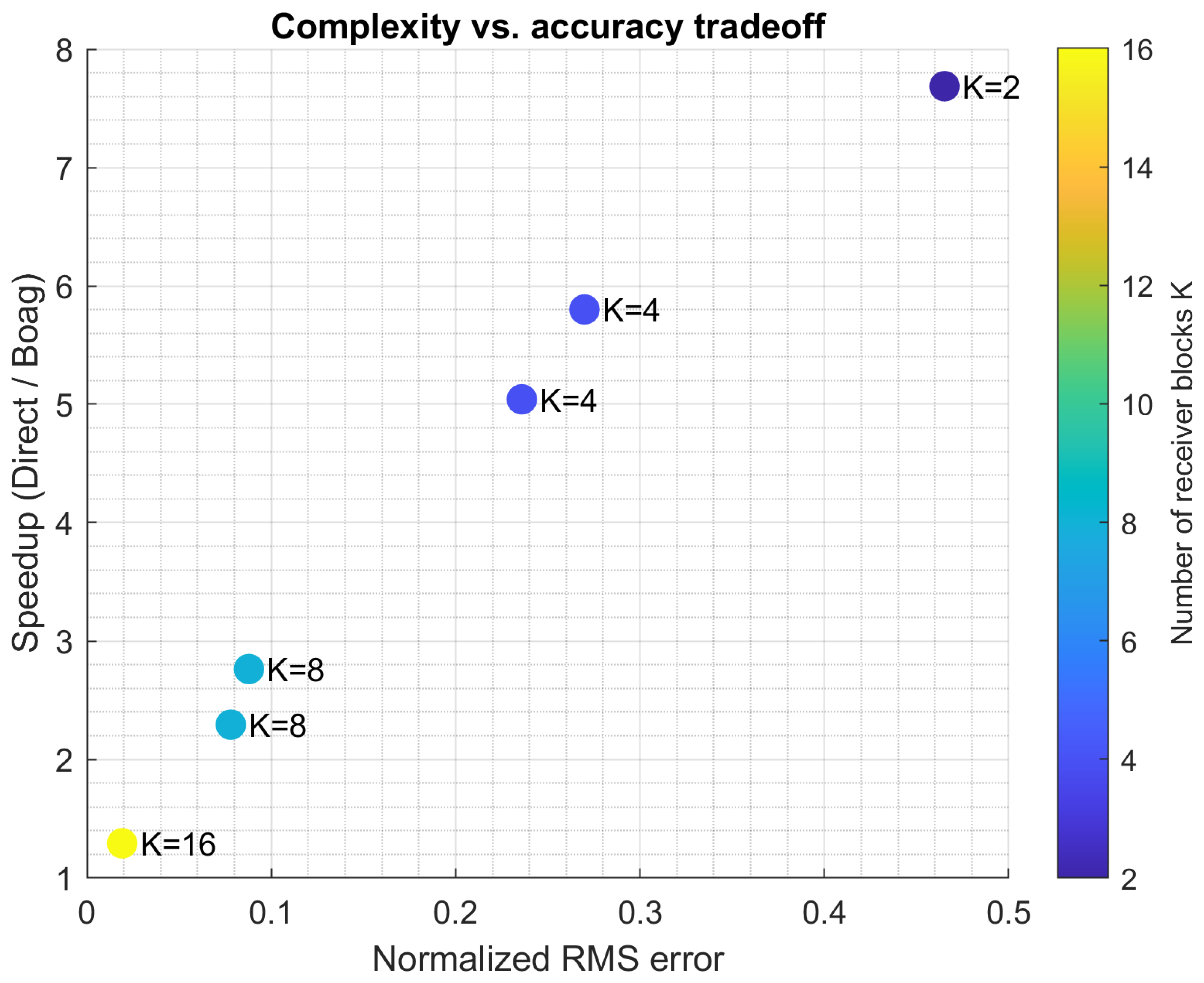
To summarize the tradeoff between computational efficiency and approximation fidelity, Fig. Figure 7 presents the measured speedup as a function of the normalized RMS error for the considered transmitter–receiver–target geometry. As expected, higher computational savings are accompanied by increased approximation error, illustrating the fundamental tradeoff between reduced evaluation time and interpolation accuracy.
8. Discussion
The results support several conclusions. First, in the static known-envelope case, time compression makes the direct matched filter particularly efficient, so an approximation is unlikely to be beneficial on very small 3D grids. Second, phase correction is essential; without it, the coarse block fields remain highly oscillatory and interpolation is ineffective. Third, the main value of the approximation idea in this setting lies not in small proof-of-concept problems but in larger-scale images where full-grid matched filtering becomes substantially more expensive.
The method is expected to degrade in at least three regimes. First, if the uncompensated or only weakly compensated block images remain highly oscillatory, the smoothness assumptions behind interpolation are violated. Second, overly aggressive coarse-grid spacing can remove local peak structure and distort the matched-filter surface. Third, strong extended-target interference or dense multipoint scattering may produce block fields whose behavior cannot be accurately represented by simple coarse-grid interpolation without adaptive refinement.
9. Conclusion
A receiver-domain-decomposition principle has been developed for near-field multistatic matched filtering with a known signal envelope and stationary target. The revised formulation reduces the problem to coherent spatial matched filtering of time-compressed data, which provides a clean baseline for evaluating phase-corrected interpolation. The study confirms that phase correction smooths low-resolution block images and is therefore the essential enabler for interpolation-based acceleration. At the same time, the experiments show that small static problems can favor direct matched filtering because the interpolation overhead dominates. The proposed framework is therefore best viewed as a scalable strategy for larger search spaces and more demanding configurations rather than as a universal replacement for direct computation.
References
- Mensa, D.L. High Resolution Radar Cross Section Imaging, 2 ed.; Artech House: Boston, MA, USA, 1991.
- Soumekh, M. A system model and inversion for synthetic aperture radar imaging. IEEE Transactions on Image Processing 1992, 1, 64–76. [CrossRef] [PubMed]
- Nilsson, S.; Andersson, L.E. Application of fast backprojection techniques for some inverse problems of synthetic aperture radar. In Proceedings of the Proceedings of SPIE, Algorithms for Synthetic Aperture Radar Imagery V, 1998, Vol. 3370, pp. 62–72. [CrossRef]
- Boag, A. A fast multilevel domain decomposition algorithm for radar imaging. IEEE Transactions on Antennas and Propagation 2001, 49, 666–671. [CrossRef]
- Haimovich, A.M.; Blum, R.S.; Cimini, L.J. MIMO Radar with Widely Separated Antennas. IEEE Signal Processing Magazine 2008, 25, 116–129. [CrossRef]
- Li, J.; Stoica, P., Eds. MIMO Radar Signal Processing; Wiley: Hoboken, NJ, USA, 2009.
- Manisali, I.; Oral, O.; Oktem, F.S. Efficient Physics-Based Learned Reconstruction Methods for Real-Time 3D Near-Field MIMO Radar Imaging. Digital Signal Processing 2024, 144, 104274. [CrossRef]
- Price, G.A.J.; Moate, C.; Andre, D.; Yuen, P. Sidelobe Suppression Techniques for Near-Field Multistatic SAR. Sensors 2023, 23, 732. [CrossRef] [PubMed]
- Masoodi, M.; Gennarelli, G.; Noviello, C.; Catapano, I.; Soldovieri, F. Performance Assessment of Multistatic/Multi-Frequency 3D GPR Imaging by Linear Microwave Tomography. Sensors 2025, 25, 6467. [CrossRef] [PubMed]
- Cheng, Q.; Zhang, Y.; Zeng, C.; Zhou, Z.; Liao, G.; Tao, H. Near-Field Target Detection with Range–Angle-Coupled Matching Based on Distributed MIMO Radar. Sensors 2025, 25, 7003. [CrossRef] [PubMed]
- Ivanenko, Y.; Vu, V.T.; Batra, A.; Kaiser, T.; Pettersson, M.I. Interpolation Methods with Phase Control for Backprojection of Complex-Valued SAR Data. Sensors 2022, 22, 4941. [CrossRef] [PubMed]
- Molaei, A.; et al. Fast Image Reconstruction for Near-Field Terahertz Imaging with Multistatic Non-Uniform Sparse Arrays. In Proceedings of the Radar Sensor Technology XXVII, 2023, Vol. 12535, Proceedings of SPIE, p. 125350Y. [CrossRef]
- Liu, F.; et al. Integrated Sensing and Communications: Recent Advances and Ten Open Challenges. IEEE Internet of Things Journal 2024, 11, 19094–19120. [CrossRef]
Figure 1.
Potential System Layout (used in the simulations).
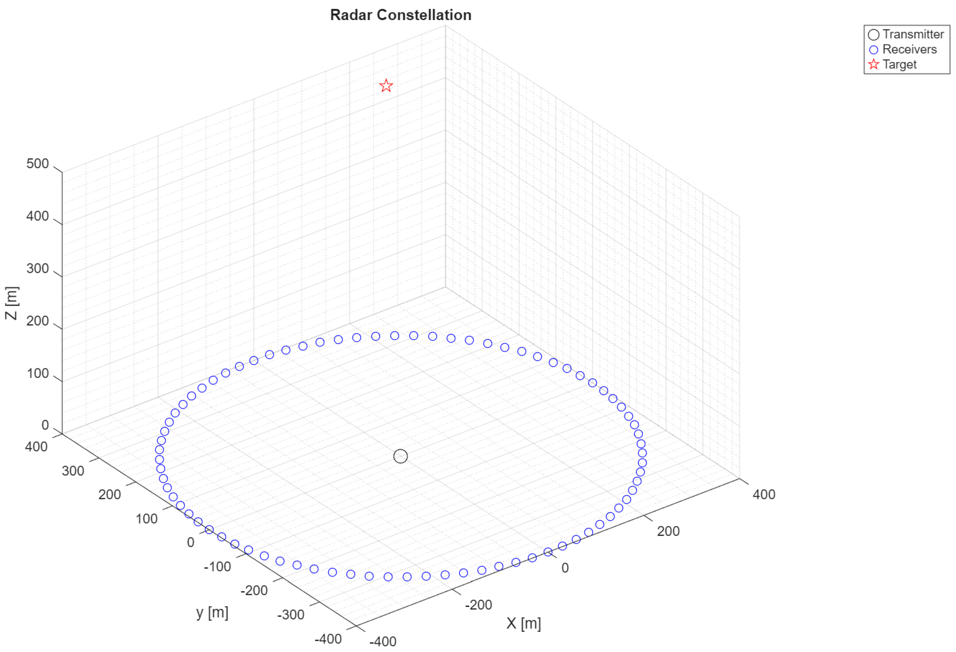
Figure 2.
Representative coarse block image before and after phase correction. The corrected phase map is visibly smoother.
Figure 2.
Representative coarse block image before and after phase correction. The corrected phase map is visibly smoother.
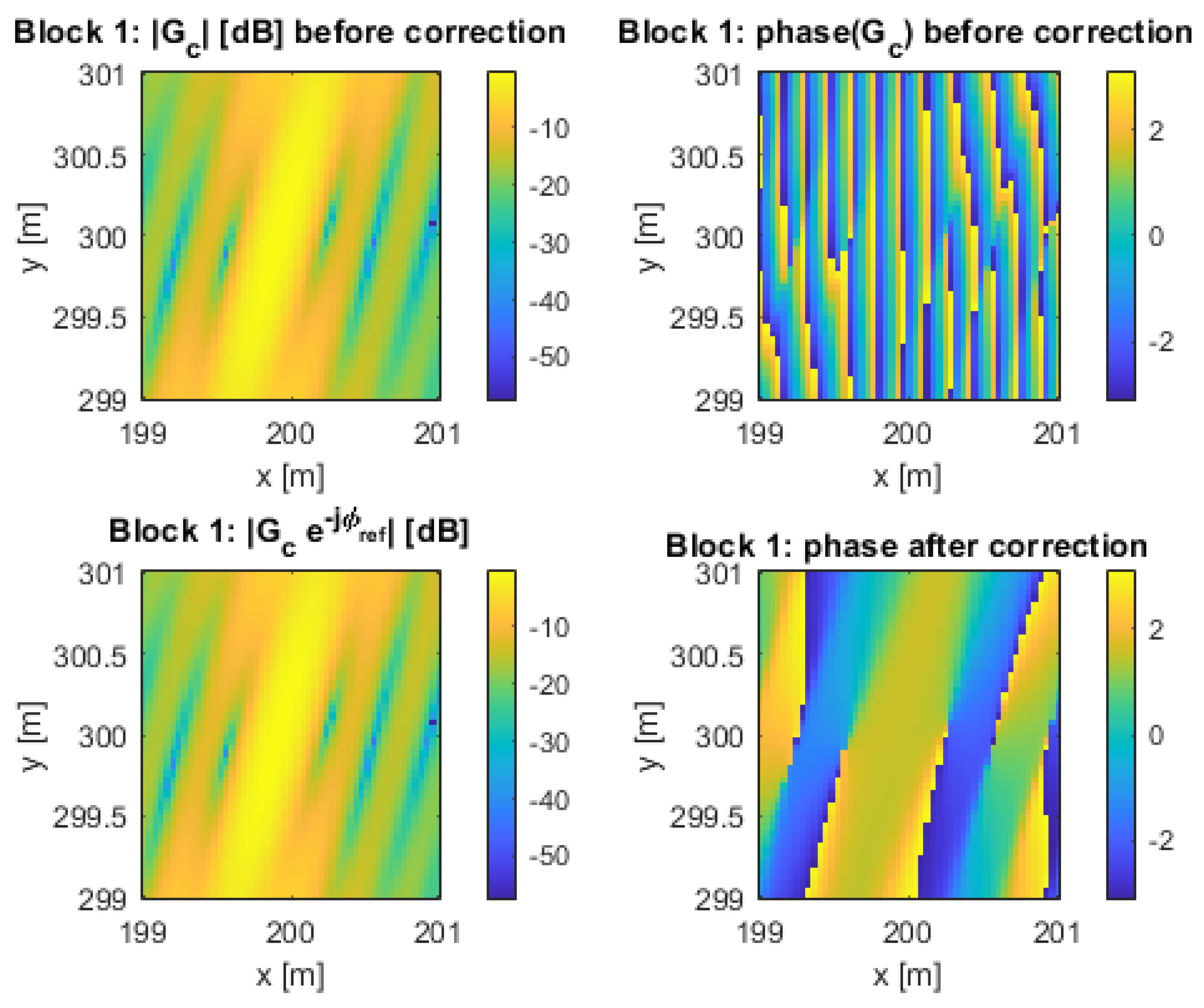
Figure 3.
One-dimensional cuts of the coarse block field before and after phase correction, illustrating reduced oscillation after compensation.
Figure 3.
One-dimensional cuts of the coarse block field before and after phase correction, illustrating reduced oscillation after compensation.
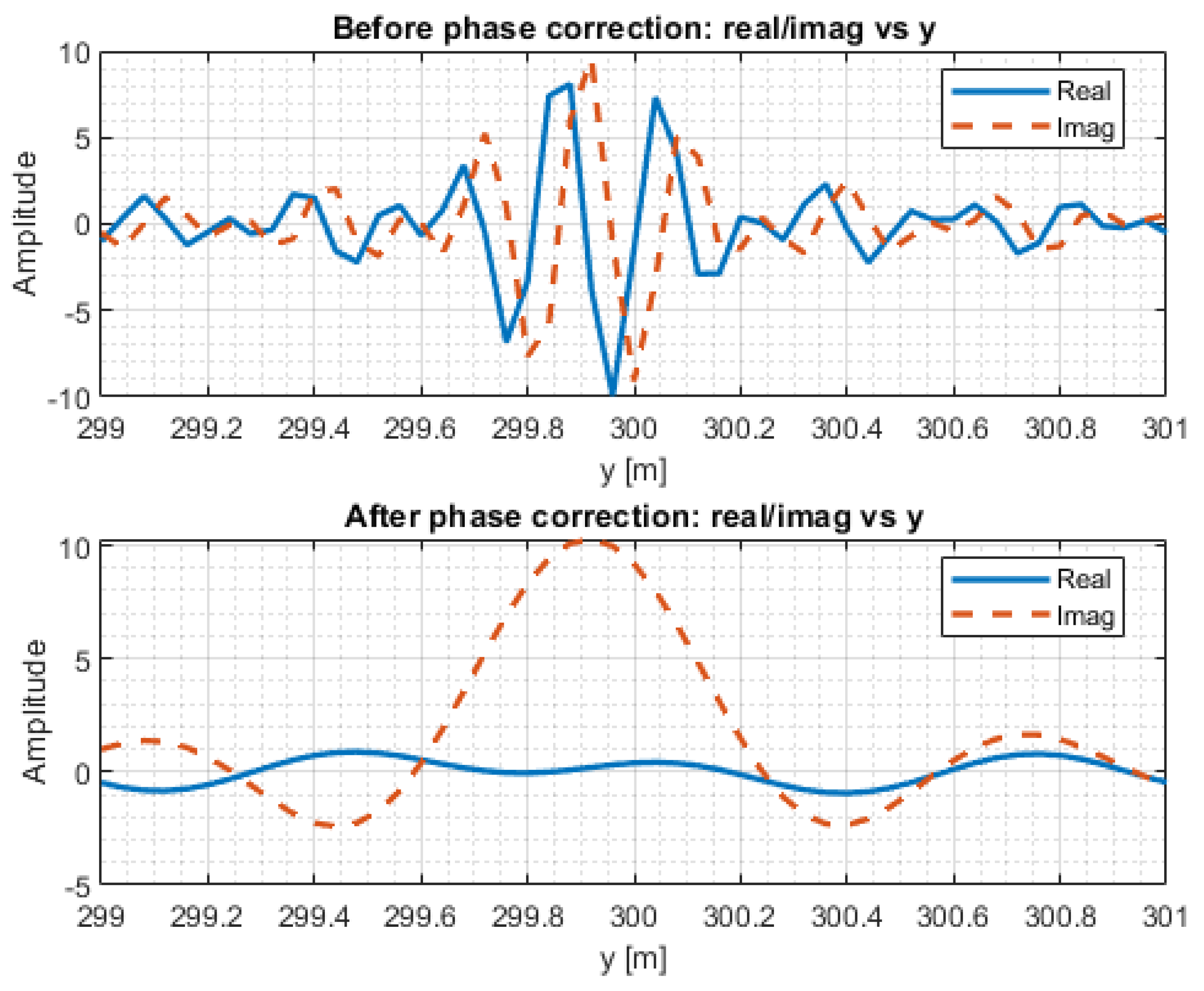
Figure 4.
Normalized score in dB versus x, with y and z fixed at their true values.
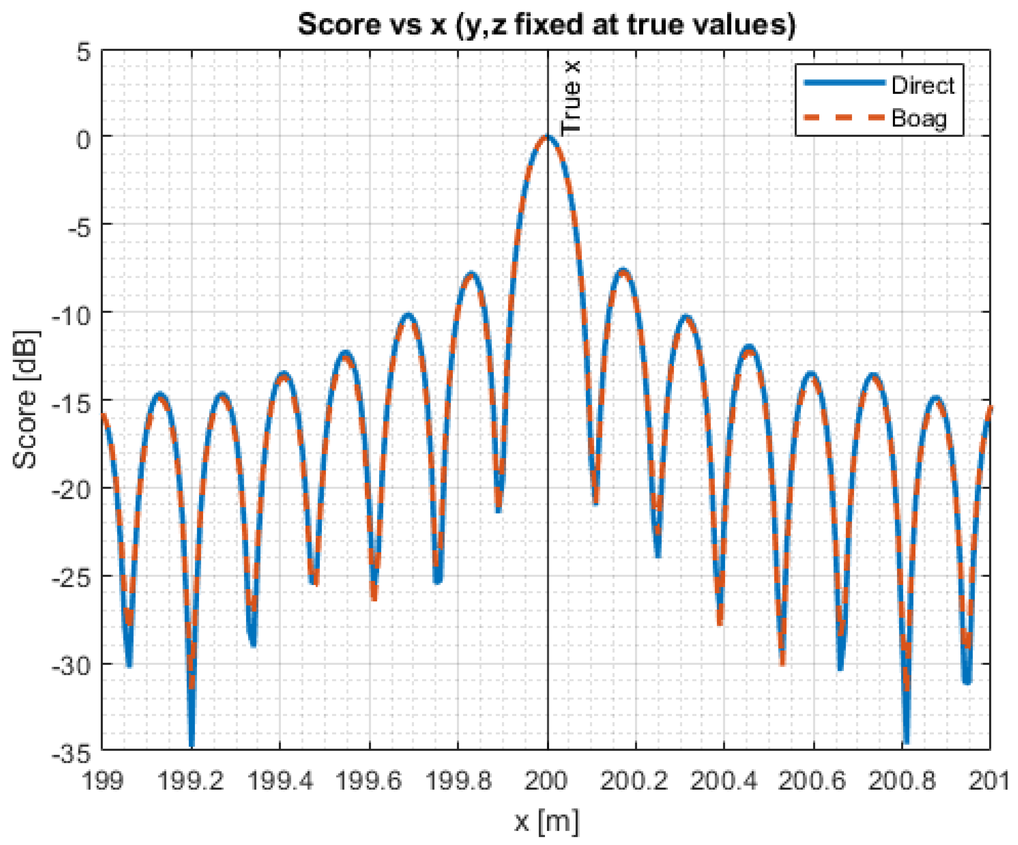
Figure 5.
Normalized score in dB versus y, with x and z fixed at their true values.
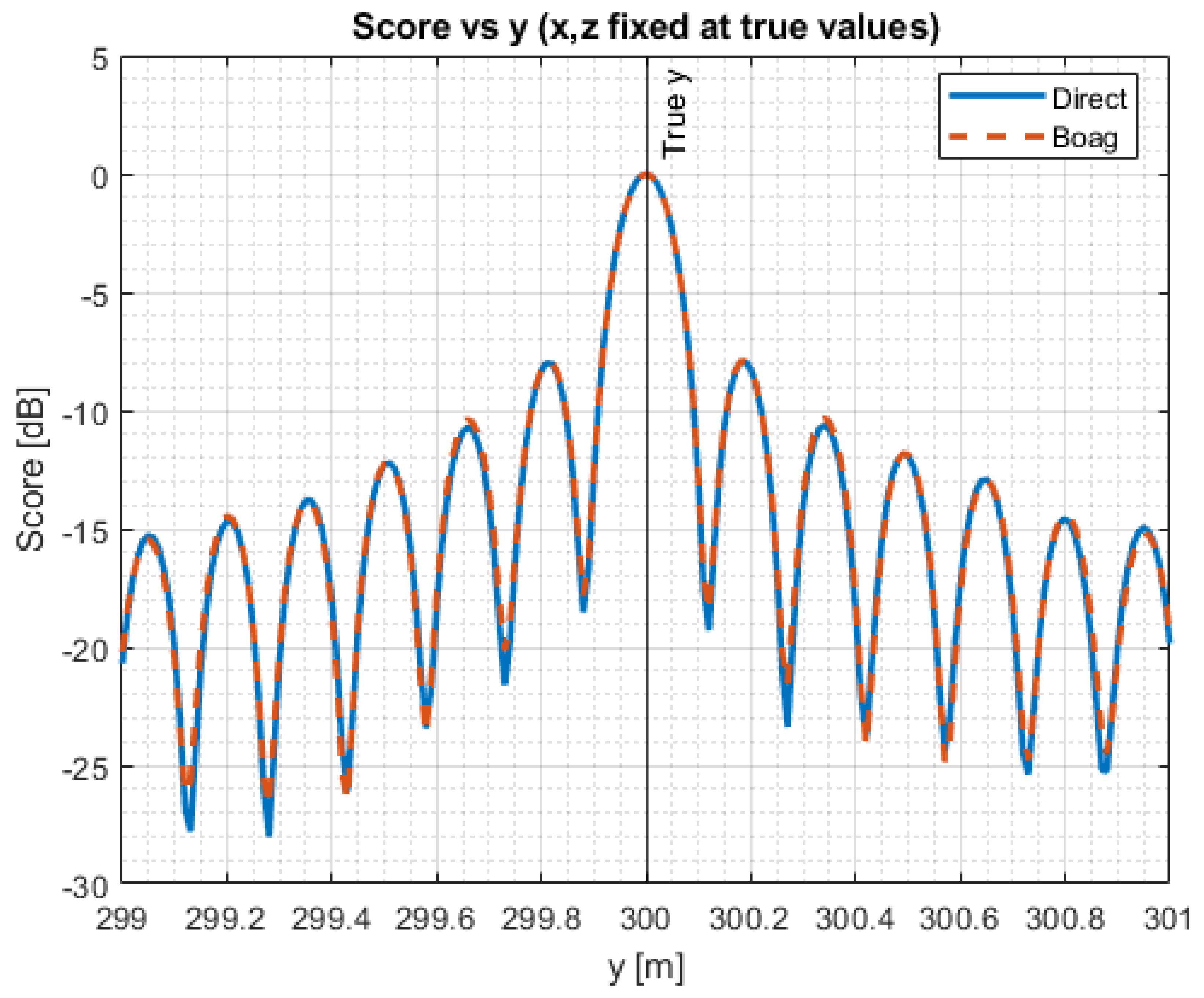
Figure 6.
Normalized score in dB versus z, with x and y fixed at their true values.
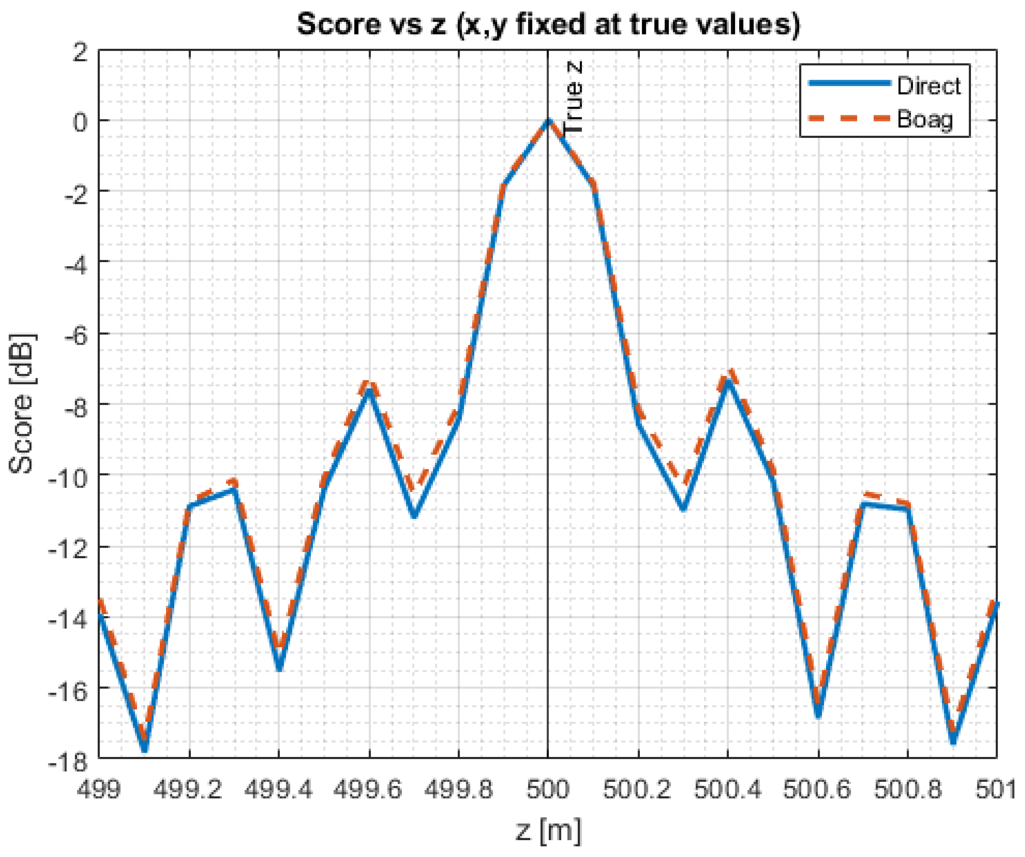
Figure 7.
Complexity–accuracy tradeoff for the measured operating point, shown as speedup versus normalized RMS error. Additional sweep results can be added to reveal the full tradeoff frontier.
Figure 7.
Complexity–accuracy tradeoff for the measured operating point, shown as speedup versus normalized RMS error. Additional sweep results can be added to reveal the full tradeoff frontier.
Disclaimer/Publisher’s Note: The statements, opinions and data contained in all publications are solely those of the individual author(s) and contributor(s) and not of MDPI and/or the editor(s). MDPI and/or the editor(s) disclaim responsibility for any injury to people or property resulting from any ideas, methods, instructions or products referred to in the content. |
© 2026 by the authors. Licensee MDPI, Basel, Switzerland. This article is an open access article distributed under the terms and conditions of the Creative Commons Attribution (CC BY) license (http://creativecommons.org/licenses/by/4.0/).
Copyright: This open access article is published under a Creative Commons CC BY 4.0 license, which permit the free download, distribution, and reuse, provided that the author and preprint are cited in any reuse.


