

Submitted:
22 July 2026
Posted:
23 July 2026
You are already at the latest version
Abstract
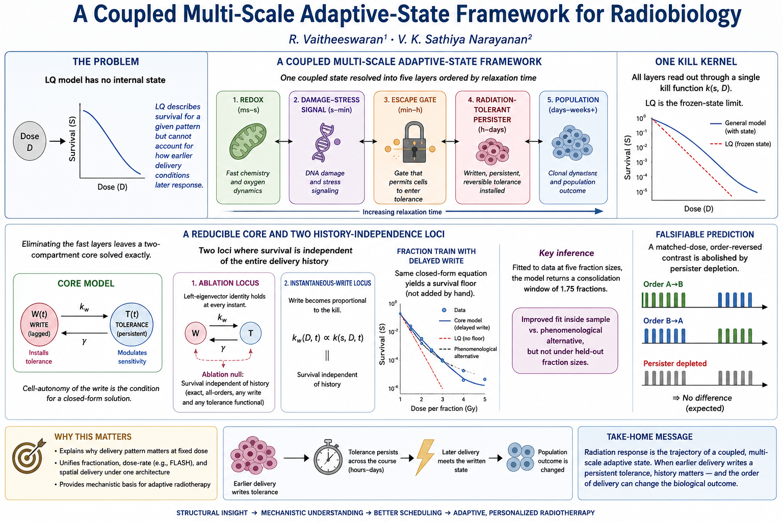
The linear–quadratic (LQ) model accumulates dose but carries no internal state, so it cannot represent how an earlier delivery conditions the response to a later one. We propose that radiation response is better treated as the trajectory of a single coupled state resolved into five layers ordered by relaxation time — redox, damage-stress signal, escape gate, radiation-tolerant persister, and population — read out through one kill kernel of which LQ is the exact frozen-state limit. Because the layer clocks separate by orders of magnitude the architecture is reducible: eliminating the fast layers leaves a two-compartment core of the lagged write that installs tolerance and the tolerance itself, on which the system is solved exactly. The resulting closed-form surviving fraction becomes independent of the entire delivery history on exactly two loci: an ablation locus, following from a left-eigenvector identity holding at every instant and therefore exact, all-orders, and independent of both the tolerance functional and the write; and an instantaneous-write locus, where the write becomes proportional to the kill. Cell-autonomy of the write is precisely the condition under which a closed form exists, and the ablation null survives even where it does not. Specialised to a fraction train under a delayed write, the same equation derives a survival floor previously added to LQ by hand; fitted to data at five fraction sizes it returns a consolidation window of 1.75 fractions and is preferred over the phenomenological alternative in sample, though not under held-out fraction sizes. The remaining results require layers the core does not contain, which is the argument for the framework and not only for the theorem. The falsifiable content is structural: a matched-dose, order-reversed contrast abolished by persister depletion.
Keywords:
radiation-tolerant persister
; linear–quadratic model
; treatment scheduling
; multi-timescale model
; adaptive radioresistance
; delivery-order effect
1. Introduction
1.1. A Kill Law with No Internal State
Radiotherapy is increasingly delivered through distinct delivery patterns — variations in dose magnitude, dose rate, temporal scheduling and spatial distribution — each of which can change the biological outcome at a fixed total dose. The linear–quadratic (LQ) model remains the workhorse: it describes how survival scales with dose for a given pattern, and its two parameters can be tuned to fit fractionation or dose-rate data (Fowler, 1989; McMahon, 2019). But LQ treats dose as a scalar and carries no internal state. It holds no variable for the condition of the tissue it is treating, and so cannot register that an earlier dose might change how a later one lands. It already mispredicts equivalence at large fraction sizes (Park et al., 2008; Brenner, 2008); more fundamentally, it offers no principled account of how one delivery pattern conditions the response to the next.
Several problems the field treats separately follow from this one absence, and they are not independent. Schedule-equivalence at matched dose, the arithmetic on which fractionation rests (Ahmed et al., 2014), fails wherever treatment induces a persistent change in sensitivity. The planning quantities built on LQ inherit its frozen-sensitivity assumption and misprice any history-dependent response. As FLASH, spatially fractionated and stereotactic regimens and their combinations proliferate (Vozenin et al., 2019; Prezado et al., 2024), whether two patterns interact has become a central question (Schneider et al., 2022), currently answered descriptively by fitting an interaction term after the fact. Each of these is a way in which a course of treatment changes the tissue it is treating, and a state-blind kill law cannot see any of them. The thread running through the symptoms is one particular state — a written, persistent, reversible tolerance that an earlier dose installs and a later dose then meets. It is not the only internal state that matters, but dose rate and spatial delivery carry narrow channels on far shorter clocks, whereas the written tolerance survives across the course and therefore threads every problem in which early delivery conditions late response.
1.2. What the Field Already Has, and What It Lacks
That radiosensitivity is dynamic is not new; it is the accumulated result of a century of work. It was first conceived as fixed by cellular identity (Bergonié & Tribondeau, 1906; Foray, 2012), then made a function of cycle position by redistribution (Sinclair & Morton, 1966; Hall & Giaccia, 2018) and of the microenvironment by reoxygenation (Gray et al., 1953; Kallman, 1972). The radioadaptive response took the decisive step: radiation itself down-modulates subsequent sensitivity, on a delay, by a mechanism distinct from sublethal repair (Olivieri et al., 1984; Wolff, 1998; Joiner et al., 2001; Scott, 2004; Di Dio et al., 2025; Krasowska et al., 2026). What none of these stages derived is what that dynamism implies for how radiation should be delivered.
Radiobiology already couples a reduced radiosensitivity to LQ in two ways: a discrete radioresistant compartment surviving each fraction (Pajonk et al., 2010; Yu et al., 2015), and a continuous distribution of radiosensitivity drifting toward its resistant tail as a protracted course removes sensitive cells preferentially (Alfonso & Berk, 2019; Lewin et al., 2018). Between them these reproduce treatment-acquired radioresistance, accelerated repopulation and fraction-size dependence, honestly and within standard LQ. But they contain exactly the two features the present construction does not. First, the resistant fraction is reached by selection: no cell changes state. Second, the response is instantaneous: no dynamics is interposed between damage and the change in sensitivity. These are precisely the conditions under which the results below are empty — a resistance that is selected rather than written leaves both populations tied to the same delivery-blind bookkeeping, and an instantaneous response is the zero-lag limit in which the second of our two nulls is reached identically. The nearest radiobiology models are therefore not rivals but the null case of the construction.
The missing ingredients — an actively written, heritable, lagged tolerance on a distinct compartment with a multiplicative back-effect on kill — are not ours to invent. In bacterial persistence, stress history writes a transiently tolerant state with a reduced but non-zero death rate, an explicit induction lag, and a survival that depends on the timing of exposure (Abbott et al., 2026). In the drug-tolerant-persister lineage a reversible, chromatin-encoded state is written by therapy, inherited across divisions, and lost when its writer is removed (Sharma et al., 2010; Russo et al., 2024), the writer supplying a handle whose inhibition re-sensitises cells on rechallenge (Dayanc et al., 2025), with cross-resistance across therapy classes (Davern et al., 2025). Li et al. (2026) show, with progressive selection excluded by single-cell imaging, that such a state is actively learned rather than selected, mediated by AP-1 with CBP/p300, encoded in cis, abolished when AP-1 is inhibited, and — most consequentially — that a prior low-dose exposure is thereby converted into resistance against a later high dose. What licenses the transfer is that radiation biology has caught up: fractionated irradiation generates a radiation-tolerant persister driving recurrence in glioblastoma (Gu et al., 2022); a colorectal persister has been isolated and shown to revert (Zhao et al., 2023); lineage tracing shows persisters arising by reprogramming rather than selection (Forissier et al., 2025); the state recurs across cancers and therapies (Ling et al., 2026; Valcz et al., 2025); the change is epigenetically written rather than mutational (Belli & Tabocchini, 2020); and the tolerance form has been measured, best captured as a multiplicative, dose-dependent modifier of the LQ parameters rather than a fixed subtraction (Van den Berg et al., 2020).
We fence the contribution against three neighbouring literatures. The optimal-control and scheduling tradition (Almquist & Banks, 1976; Bortfeld et al., 2015; Gouw et al., 2024; Fu et al., 2026) establishes that when tumour state evolves the optimal schedule is non-uniform, but always as a computed optimum for a given parameter set, never as a closed-form identity holding across the parameter manifold; Ayati et al. (2016) characterise when non-interacting modalities decouple, where we characterise the regime in which they do not. The operator machinery for two-state linear systems is classical (Magnus, 1954; Wei & Norman, 1963; Blanes et al., 2009) and we treat it as presentational. The adaptive-therapy lineage (Gatenby & Brown, 2020; Zhang et al., 2017; Gillies et al., 2012) develops schedule-dependence in two-population models, but there it arises from differences in fitness under selection, whereas ours arises from a difference in kill hazard; the state-based tradition now includes multiscale epigenetic-instability models (Wang et al., 2025) and simulation-based accounts (Scheidegger et al., 2013; Powathil et al., 2013), which forfeit the closed form.
1.3. What This Paper Adds
Because the missing state is a single thread, the remedy is one structural change rather than a patch per symptom: give the kill law an internal state, so that history-dependent effects become perturbations of one coupled object. Because the processes that write and clear that state occupy timescales separated by orders of magnitude, the state is not a single variable but a small hierarchy of coupled layers, reducible precisely because the clocks separate. Section 2 specifies that architecture; Section 3 performs the reduction and solves the core exactly; Section 4 confronts the fractionation specialisation with published data; Section 5 develops the results requiring layers the core does not contain; Section 6 reads the delivery modalities through the architecture; Section 7 and Section 8 discuss status and falsification. We do not claim to explain an observation already in hand — the discriminating experiment has not been run. We derive a structure, show what it forces, fit its fractionation specialisation to the one dataset that can constrain it, and specify the experiment that would confirm or refute the mechanism.
2. The Coupled Multi-Timescale Model
We treat radiosensitivity as a state rather than a fixed pair of coefficients. Response is read out through a single kill kernel acting on a coupled state, so the LQ coefficients become functions of that state. The state resolves into five layers ordered by relaxation time, coupled in both directions, and evolving throughout treatment — including between deliveries — so that it carries the history of what has been delivered.
2.1. State and Timescales
The layers are not chosen for mathematical convenience. Each corresponds to an established radiobiological process on a distinct clock, each is grounded in a separate experimental literature (Table 1), and they are split by the timescale on which they relax, because that separation licenses the reduction of Section 2.4 and fixes which layer can carry history between fractions. Treatment enters as the dose rate Ḋ(t) ≥ 0, with cumulative dose D(t).
The B layer is grounded in radiation directly rather than by analogy: radiation reprograms surviving cells into a heritable, slow-cycling, tolerant state that drives recurrence (Gu et al., 2022; Forissier et al., 2025; Zhao et al., 2023). Critically, the molecular writer differs by context — NF-κB/YY1 in glioblastoma, LRP4/YAP in breast, AP-1 with CBP/p300 in the drug analogue (Li et al., 2026), a multi-phase network in head-and-neck carcinoma (Ling et al., 2026) — while the architecture is conserved: a treatment-induced, transcriptionally written, heritable, pharmacologically inhibitable tolerance step. That conserved-form, divergent-molecule pattern is recognised at the level of cross-cancer synthesis (Russo et al., 2024), and is why the framework carries the persister as one coarse-grained variable rather than any specific effector.
2.2. The Kill Kernel and the Linear–Quadratic Limit
The instantaneous log-kill hazard on a non-persister clonogen is the time derivative of the LQ exponent, with the linear coefficient set by oxygenation:
Persister clonogens experience the same hazard reduced by a tolerance factor, r h(t) with 0 ≤ r < 1. Integrating over a state that does not evolve during delivery returns the classical form exactly,
so LQ is the frozen-state limit of the kernel rather than an approximation to be refined pointwise, and departures arise exactly when a layer evolves during treatment. The framework does not compete with LQ: it contains it, and identifies when it is exact.
−ln S = αD + βD²
2.3. Couplings, and Why the Back-Arm Is Load-Bearing
Writing the induction rate as k(t) = κs(t), the populations evolve during a delivery window as a linear time-varying system driven by the slaved redox and signal layers and gated by the escape variable. The two-compartment generator is lower-triangular,
with the stress signal a lagged image of the damage rate and the induction proportional to it,
Between deliveries the system adds the slow terms — net proliferation of each compartment, persister death, and escape-gated reseeding — all quasi-static over any single delivery window and therefore absent from the theorem.
The coupling is bidirectional, and the back-arm carries the results. Bottom-up, irradiation drives the cascade x → α → damage → s → k → Np, which writes the persister, while damage gates escape through the interferon variable. Top-down, the persister acts back on the kill law through the tolerance ratio r. The back-arm is not decorative: it is exactly the tolerance gap every history-dependent result requires, since a purely bottom-up, write-only cascade (r = 1) leaves the kernel unmodified and every order, timing and interaction effect vanishes identically — the content of the ablation null of Section 3.3. Bidirectionality is a necessary condition for the framework’s predictions, not an optional refinement.

Table 2.
Couplings and their biological basis. The S→B write is the keystone; the B→kill tolerance is the back-arm carrying every history-dependent result. The coupling marked (proposed) is a hypothesis to be tested.
Table 2.
Couplings and their biological basis. The S→B write is the keystone; the B→kill tolerance is the back-arm carrying every history-dependent result. The coupling marked (proposed) is a hypothesis to be tested.
| Coupling | Model term | Biological basis | Key references |
|---|---|---|---|
| S → B (write; keystone) | k = κs | stress signalling drives the persistent transition; transcriptional write-and-inherit step | Li 2026; Gu 2022; Mothersill & Seymour 2001 |
| B → kill (tolerance back-arm) | r in r h | persister state lowers radiosensitivity to a subsequent dose; multiplicative and dose-dependent in fractionation data | Zhao 2023; Van den Berg 2020; Sharma 2010 |
| B → E (reseeding) | νρ(a)Np | persister reservoir buds near-parental progeny that repopulate; reversion | Zhao 2023; Ling 2026 |
| A gates B escape | ρ(a) | interferon / budding toggle releases progeny; bistable | Zhao 2023 |
| M → kill / write | α(x); −χḊ | oxygenation sets sensitivity; radiolytic depletion is the FLASH channel; reactive-oxygen handling couples M to B | Pratx & Kapp 2019; Forissier 2025; Russo 2024 |
| M → S (proposed) | redox priming | a redox excursion primes the write | Di Dio 2025 (proposed) |
2.4. The Reduction Tower
With the ordering τx ≪ τs ≪ τa ≪ τw ≲ τb ≪ τE, successive quasi-steady-state elimination freezes each fast layer in turn: redox, signal and escape gate are slaved, leaving the persister as the slow manifold and the population frozen on the treatment timescale. With fast reversion and no induction the second compartment is empty and survival reduces to the LQ base of the tower. The first correction to the persister manifold is proportional to the persister lifetime times the rate of change of the induction profile, so departure from LQ is gated by how fast the schedule switches relative to that lifetime: the persister matters only when reversion is slow and the schedule is switching.
The two-compartment substrate on which Section 3 proves its results is therefore the singular-perturbation reduction of the five-layer state onto the write-and-tolerance core, and each symbol acquires there a definition the reduced model can only name: h is the redox-set kill rate through α(x), k and τw are the S→B coupling, r is the B→kill arm. The architecture is chosen not to be complete but to be reducible, and the reduction is what makes the problem solvable in closed form; were the escape and persister clocks comparable, the eliminated cross-terms would re-enter and no closed form would survive.
Table 3.
collects the symbols, with the values used to generate the results; these are illustrative, chosen to place the write lag at the scale of the course, and are not calibrated to any dataset.
Table 3.
collects the symbols, with the values used to generate the results; these are illustrative, chosen to place the write lag at the scale of the course, and are not calibrated to any dataset.
| Symbol | Meaning | Value / range used |
|---|---|---|
| α, β | LQ linear (lethal) and quadratic (sublethal) coefficients | 0.30 Gy⁻¹, 0.03 Gy⁻² illustrative; 0.127, 0.087 fitted (§6.5) |
| D, Ḋ | cumulative dose; dose rate | 8 Gy course; 60 Gy / 30 fx (clinical); scanned |
| h(t) | instantaneous kill hazard, Eq. 1 | Derived |
| Ns, Np | sensitive and persister surviving fractions | state; N(0) = (1, 0) |
| R | tolerance ratio (persister / sensitive hazard) | 0 ≤ r < 1; 0.5 illustrative, scanned; 0.063 fitted (§6.5) |
| g(h) | persister hazard functional | rh (mult.); additive; saturating (Figure 3) |
| k(t) | sensitive → persister write rate, Eq. 3 | Derived |
| s(t) | write signal (low-pass of hazard) | Derived |
| τw | write lag (consolidation time) | 0.15 course units; scanned |
| γ, κ | signal gain; write coupling strength | 1.0; 0.3 illustrative; κ = 0.086 fitted (§6.5) |
| H(t), K(t) | cumulative hazard ∫h; cumulative write ∫k | Derived |
| S(T) | total surviving fraction, Eq. 4 | — |
| T | end of treatment course | 1 (normalised) |
| Ω, Ω2, J | Magnus operator; 2nd-order term; commutator integral, Eq. 9 | — |
| L | per-fraction log-kill, αd + βd² (Corollary 2) | Derived |
| A, B, C | per-fraction factors e⁻ᴸ, e⁻ʳᴸ, e⁻ᵏᴸ (Corollary 2) | Derived |
| nw, M | consolidation delay in fractions; fractions with write active | 1.75 fx fitted, 95% interval [1.25, 2.50] ≈ 2.5 d at 5 fx/wk (§6.5) |
3. The Exact Survival Law and Its Scheduling Nulls
This section works on the reduced core: two populations, the lagged write that couples them, and the tolerance gap. Everything here is exact for that system.
3.1. Axioms
Writing N = (Ns, Np)T, the core dynamics Eq. 3 are linear and time-varying, Ṅ = A(t)N, with lower-triangular generator, we solve this system in closed form, exhibit LQ as its frozen limit, and derive the two scheduling nulls. Throughout, and and H = H(T), K = K(T) with T representing the end of the treatment course.
The construction rests on five statements.
(A1) The clonogenic population resolves into a sensitive and a persister compartment killed by the same delivery at different rates.
(A2) Transfer runs one way, at a rate k(t) ≥ 0; reversion is frozen within the delivery window.
(A3) The persister hazard is a scalar multiple of the sensitive hazard, g(h) = rh with 0 ≤ r ≤ 1; the nulls require only the ablation boundary g(h; r = 1) = h. A3 is the one assumption whose form is unsettled in radiation.
(A4) The write is a causal low-pass image of the hazard with finite lag τw > 0, as in Eq. 4.
(A5) The kill kernel is local in time, so all history is carried by the written state and not by the kernel. A5 is what excludes an explicit sublethal-repair convolution, deliberately (Section 7.3);
3.2. Lemma 1 (LQ Recovery)
If the write is absent (k ≡ 0) then Np ≡ 0 and S(T) = exp[−H(T)] with H = ∫h dt = αD + βD². LQ is recovered exactly, for any schedule, and is therefore the frozen-state limit of the construction rather than a competitor to it.
3.3. Theorem: The Closed-Form Surviving Fraction and Its History-Free Loci
Let H(t) = ∫₀ᵗ h, K(t) = ∫₀ᵗ k, and let S = Ns + Np be the total surviving fraction from unit initial sensitive population. Then, for any delivery schedule and any non-negative write,
(i) Exactness. Because the generator of Eq. 3 is lower-triangular, the sensitive equation closes on itself and integrates to Ns = exp[−(H+K)]; substituting into the persister equation and applying the integrating factor e^{rH} gives Eq. 5 by quadrature. No expansion, truncation or timescale approximation enters. We have verified Eq. 5 against direct numerical integration of the full three-state system on irregular multi-pulse schedules, to a relative error of order 10⁻¹⁴.
(ii) The ablation locus. At r = 1 the surviving fraction collapses to S = e−H(T), independent of the write, of its lag, and of the entire delivery history. The reason is stronger than a cancellation in Eq. 5. Writing the generator as A(t), the row vector 1ᵀ = (1, 1) satisfies
so that d(1ᵀN)/dt = −h(t)(1ᵀN) pointwise: the total population obeys a scalar equation with no reference to k whatsoever. This is a left-eigenvector identity holding instantaneously, not an integrated coincidence. The collapse is therefore exact, holds to all orders in any time-ordered expansion of the propagator, and is independent of the functional form of the tolerance and of the write; it survives dose-dependent r(D), an arbitrary causal write, and any schedule. We have confirmed it across all 120 orderings of a five-pulse irregular schedule, with a spread of 3 × 10⁻¹⁴.
1ᵀ A(t) = −h(t) 1ᵀ at every instant, when r = 1
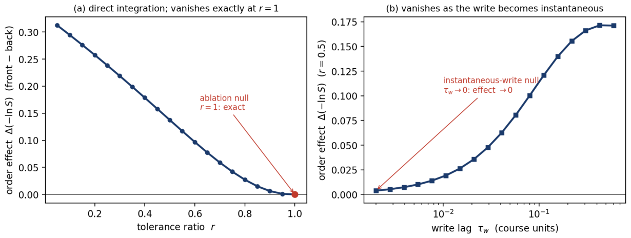
(iii) The instantaneous-write locus. As τw → 0 the filter of Eq. 4 becomes an identity, so k → κγh and K(t) = κγH(t) as functions of time. Every term of Eq. 5 then depends on the schedule only through H, and survival is again a function of total dose alone. Numerically the spread across orderings falls linearly in τw, by a factor of 234 between τw = 5 × 10⁻² and 10⁻⁵.
(iv) Genericity. With the write active (κ > 0), finite lag, and 0 ≤ r < 1, the collapse fails: direct integration across families of equal-dose schedules gives a non-zero spread throughout the interior. In particular r = 0 is not a null — an immortal persister still leaves survival schedule-dependent through K(t). A third collapse, κ → 0, is the degenerate absence of the mechanism rather than a locus of it. The history-free set is exactly the two loci above, and they are of different kinds: the ablation null is topological, saying that with no tolerance gap there is no second compartment to carry history; the instantaneous-write null says that a memory with no lag is not a memory. Between them they bracket the mechanism to the regime where a tolerance gap and a finite lag coexist — precisely the regime the selection-and-instantaneity models of Section 1.2 exclude by assumption.
Figure 1.
The two nulls, computed exactly. Order effect (log-kill of a front-loaded delivery minus its exact time reverse) obtained by direct integration of the two-compartment system, not from any truncated expansion. (a) Against the tolerance ratio r: the effect grows as the persister becomes more tolerant and vanishes exactly at the ablation locus r = 1. (b) Against the write lag τw on a logarithmic scale: the effect vanishes as τw → 0, the instantaneous-write locus.
Figure 1.
The two nulls, computed exactly. Order effect (log-kill of a front-loaded delivery minus its exact time reverse) obtained by direct integration of the two-compartment system, not from any truncated expansion. (a) Against the tolerance ratio r: the effect grows as the persister becomes more tolerant and vanishes exactly at the ablation locus r = 1. (b) Against the write lag τw on a logarithmic scale: the effect vanishes as τw → 0, the instantaneous-write locus.
3.4. Corollary 1: Write Generality and the Autonomy Boundary
Part (i) uses only that k(t) is a known function of time along the delivery, so Eq. 5 and both nulls hold unchanged for saturating, thresholded, dose-rate-dependent or memory-kernel writes — any causal functional of the cell’s own hazard. If instead the write is a feedback functional of the persister population, the sensitive equation no longer closes and the closed form is lost; the ablation null nevertheless survives, because Eq. 6 is a property of the generator’s column sums and is untouched by how k is generated. The null does fail under collective killing, where the persister carries an additional death term b not proportional to the sensitive hazard: then 1ᵀA = (−h, −h − b), not a multiple of 1ᵀ, and no scalar equation for the total exists at any r. Cell-autonomy is therefore precisely the condition under which a closed form exists, and the ablation null is strictly more robust than the closed form accompanying it — which matters experimentally, since the ablation contrast can be run without committing to any write mechanism.
3.5. Corollary 2: Fractionated Delivery Under a Delayed Write
Specialise to a train of n equal fractions each of log-kill L = αd + βd², with the write acting between fractions and inactive until a consolidation length nw of fractions has been delivered. Put A = e−L, B = e−rL, C = e−κL, M = n − nw. Then
SF(n) = e−nL (n ≤ nw), SF(n) = e−nwL [ (AC)M + A(1−C) ((AC)M−BM)/(AC−B) ] (n > nw)
Eq. 7 is Eq. 5 evaluated on a pulse-train hazard with a delayed write, the persister integral having become a geometric sum. We have verified it against direct fraction-by-fraction propagation over 2,880 combinations of (n, nw, r, κ, L) with no mismatch at 10⁻¹⁰, and confirmed that it inherits the ablation null exactly. Its late-time behaviour is therefore analytic: for a fully protected consolidated state (r = 0, B = 1) with AC < 1, letting M → ∞ gives a finite survival floor,
so the level at which a fractionation curve settles falls exponentially in the per-fraction log-kill, with a slope set by the consolidation window. This is where the framework becomes quantitatively testable, because a floor of exactly this shape has previously been inserted into LQ by hand (Van den Berg et al., 2020); here it is derived and its exponent predicted rather than fitted. For r > 0 no true floor exists and the same expression gives a slow geometric decline beneath a constant amplitude, so comparisons with data are made at the fraction number actually measured.
SF∞ = e−nw L · A(1−C)/(1−AC) , ln SF∞ ≈ −(nw+1) L + ln(κL) − ln(1−e−(1+κ)L)
3.6. The Order Effect Between the Loci: Exact and Approximate Components
Away from the nulls, delivery order alters kill, and it is important to be precise about which features of this effect are theorems and which are not. Expanding Eq. 5 to first order in the tolerance gap (1−r) gives the order-dependent part of the log-kill; organised through the Magnus expansion of the propagator, exp(Ω) with Ω = Ω₁ + Ω₂ + …, the second-order term is the operator commutator
where
with E₂₁ the unit matrix in the (2,1) position; the commutator
is nonzero precisely because the write lags the kill, which is why τw → 0 is a null.
[ A(t₁), A(t₂) ] = (1−r)(h₁k₂−h₂k₁) E₂₁
We stress, however, that Ω₂ is not the whole order effect: because the write k is a causal functional of the hazard, the write integral K is itself order-dependent, so the first Magnus term Ω₁ contributes an order effect of the same order and opposite sign. The single scalar ½(1−r)J is therefore not a closed-form law for the effect, and we do not use it as one: neither its sign nor its magnitude should be read as an approximation to the exact difference, which is computed throughout from Eq. 5 or Eq. 7. What the commutator does establish exactly is that it vanishes identically only on the two loci themselves — at the ablation boundary, and where the write becomes proportional to the kill — which is the structural reason the instantaneous-write locus is a null.
3.6. What the Theorem Does Not Give
Away from the two loci the construction predicts that delivery order changes outcome, and Eq. 5 computes that change exactly for any given pair of schedules. It does not supply a closed-form law for the size of the effect. It is tempting to read the second-order term of a time-ordered expansion of the propagator — for this generator proportional to (1 − r) times a single commutator integral — as such a law. It is not one, and we do not use it as one: because the write is itself a causal functional of the hazard, the first-order term carries an order dependence of the same size and opposite sign, so neither its sign nor its magnitude approximates the exact difference. What the commutator does establish exactly is that it vanishes identically only on the two loci themselves. All order effects quoted here are computed from Eq. 5 or by direct integration.
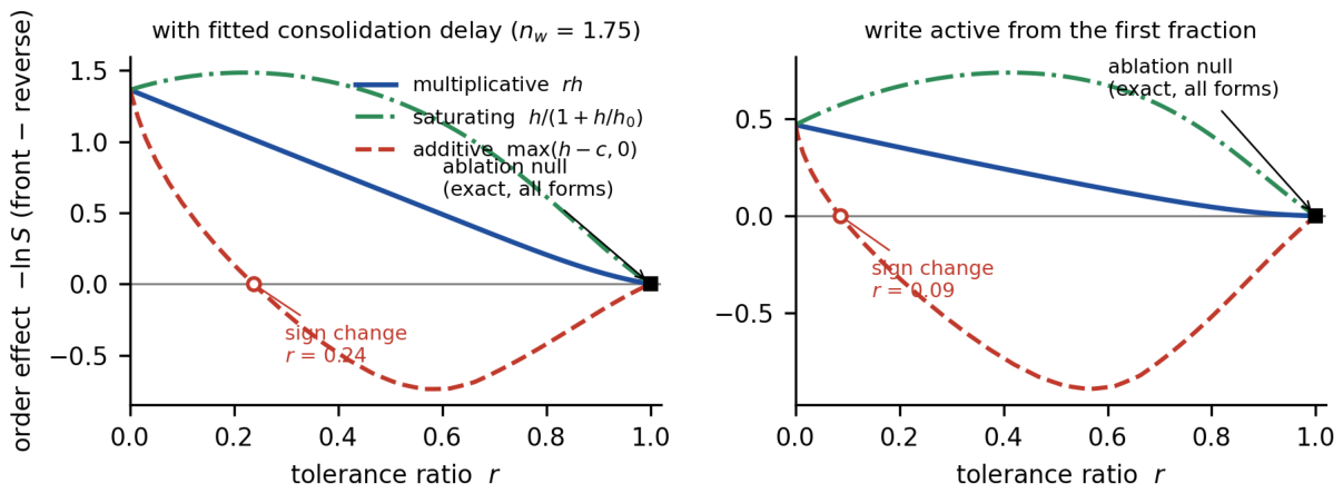
Nor is the direction of the effect a theorem. The nulls hold for any tolerance functional; the sign does not. Multiplicative and saturating tolerance make front-loaded delivery kill more at every tolerance ratio, whereas additive tolerance reverses the sign — but only where the tolerance gap is wide, above r ≈ 0.24 under the fitted consolidation delay (Figure 3). Below that threshold all three forms agree, so the sign of the order effect identifies the functional form only in the wide-gap regime, and not at the tolerance ratio the fractionation fit of Section 4 returns. The form the radiation data indicate is multiplicative (Van den Berg et al., 2020), giving front-loading. For a twenty-fraction course totalling 40 Gy whose fraction sizes fall linearly from 3.0 to 1.0 Gy, delivered large-to-small against its exact time reverse, the difference in −ln S at the fitted parameters of Section 4 is +1.27 — about 10 Gy of biologically effective dose on a course of roughly 100 Gy, or a shift of about 4 Gy delivered in 2 Gy fractions. At r = 1 it is identically zero (Figure 2).
Figure 2.
The order effect at clinical fractionation. A 60 Gy course in 30 fractions delivered front-loaded against its exact time reverse (identical fraction-size multiset, identical total dose). At the ablation locus r = 1 the two surviving fractions coincide to machine precision; at r = 0.5 they diverge by 0.67 in −ln S, front-loading producing the greater kill. The contrast isolates delivery order from fraction size.
Figure 2.
The order effect at clinical fractionation. A 60 Gy course in 30 fractions delivered front-loaded against its exact time reverse (identical fraction-size multiset, identical total dose). At the ablation locus r = 1 the two surviving fractions coincide to machine precision; at r = 0.5 they diverge by 0.67 in −ln S, front-loading producing the greater kill. The contrast isolates delivery order from fraction size.
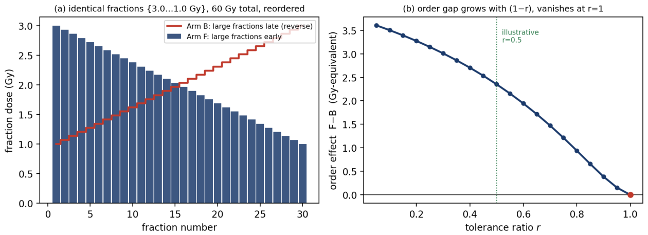
Figure 3.
The nulls are form-independent; the direction is not, and only above a threshold. Order effect against tolerance ratio for three tolerance functionals, each calibrated to the same total persister protection over the course. All three vanish exactly at r = 1. Multiplicative and saturating tolerance make front-loading kill more at every r; additive tolerance reverses the sign, but only above r ≈ 0.24 with the fitted consolidation delay (left) or r ≈ 0.09 with the write active from the first fraction (right). Below those thresholds — which includes the tolerance ratio the fractionation fit returns — all three forms agree in sign, so the sign of the order effect discriminates the functional form only when the tolerance gap is wide.
Figure 3.
The nulls are form-independent; the direction is not, and only above a threshold. Order effect against tolerance ratio for three tolerance functionals, each calibrated to the same total persister protection over the course. All three vanish exactly at r = 1. Multiplicative and saturating tolerance make front-loading kill more at every r; additive tolerance reverses the sign, but only above r ≈ 0.24 with the fitted consolidation delay (left) or r ≈ 0.09 with the write active from the first fraction (right). Below those thresholds — which includes the tolerance ratio the fractionation fit returns — all three forms agree in sign, so the sign of the order effect discriminates the functional form only when the tolerance gap is wide.
4. The Fractionation Specialisation Against Data
Section 2 and Section 3 are uncalibrated by design: the two nulls follow from the algebra and hold for every admissible parameter value, so neither can be tuned into or out of existence. This section is separate in kind. Here the specialisation of Corollary 2 is fitted to one cell line, and the parameters it returns are calibrated quantities carrying the usual liabilities. We keep the two apart, and the falsifiable content we claim is the structural part.
4.1. The Observations, and the Treatment of Radiosensitivity
Van den Berg et al. (2020) irradiated seven cell lines with repeated equal fractions and followed clonogenic survival fraction by fraction. We use their U-251MG glioblastoma series, the only one delivered at five fraction sizes — 1.8, 2.0, 2.5, 3.0 and 4.0 Gy, a 2.2-fold range — giving 68 survival points digitised from the published figures. Two features must be explained: survival falls steeply over the first few fractions and then settles, at 1.8 and 2.0 Gy reaching a level near 0.8 to 0.9 per cent and staying there, roughly 3.6 orders of magnitude above the pure-LQ prediction using the radiosensitivity measured in the same cells; and that settled level depends strongly on fraction size, falling by a factor of 84 between 1.8 and 4.0 Gy at five fractions.
The same study reports a single-dose curve for the same cells, giving α = 0.116 Gy⁻¹ and β = 0.050 Gy⁻² (α/β = 2.32 Gy). We use it in two ways, because two questions are at stake: whether an expression can describe the fractionation data requires letting radiosensitivity move, whereas whether it can reproduce them using the radiosensitivity of the same cells does not. One complication should be noted: the first fraction of the fractionation series is already more lethal than the single-dose assay predicts, by 0.53 to 0.73 in survival ratio, an assay discrepancy neither expression explains.
4.2. Fit and Model Comparison
We compare the specialisation of Eq. 7 (Model M; five parameters α, β, κ, nw, r) against the phenomenological expression of Van den Berg et al. (2020), in which an adaptive floor (α/β)−(d+1) is added to LQ survival by hand (LQAR; two parameters). Both are fitted to the same 68 points by least squares in log₁₀.
Table 4.
Comparison of the two expressions on identical data (68 points) in three regimes. Regime (i) places both on the same footing and is the comparison of primary interest; regime (ii) asks whether either reproduces the fractionation data using the radiosensitivity measured in the same cells; regime (iii) holds out whole fraction sizes in turn. Percentages are relative to the source study’s own single-dose assay.
Table 4.
Comparison of the two expressions on identical data (68 points) in three regimes. Regime (i) places both on the same footing and is the comparison of primary interest; regime (ii) asks whether either reproduces the fractionation data using the radiosensitivity measured in the same cells; regime (iii) holds out whole fraction sizes in turn. Percentages are relative to the source study’s own single-dose assay.
| Regime | LQAR | Model M |
|---|---|---|
| (i) Both free — RMS in log₁₀ | 0.184 | 0.159 |
| (i) Akaike / Bayesian criterion | −226.3 / −221.9 | −240.3 / −229.2 |
| (i) Fitted α (measured 0.116 Gy⁻¹) | 0.220 (+89%) | 0.127 (+9%) |
| (i) Fitted α/β (measured 2.32 Gy) | 4.35 (+88%) | 1.45 (−37%) |
| (ii) Both held to measured α, β — RMS | 0.769 | 0.279 |
| (ii) Overprediction of observed survival | 8.7–20.9× | — |
| (iii) Held-out fraction sizes — RMS | 0.198 | 0.211 |
| Fitted persister parameters | — | nw = 1.75 fx [1.25, 2.50]; κ = 0.086; r = 0.063 |
Three things follow. On matched footing Model M is preferred on every in-sample criterion, including a curve-clustered Vuong test (Z = +2.51, p = 0.012) and both information criteria; the Bayesian criterion penalises five parameters against two and still prefers it, so the ranking is not an artefact of parameter counting. More informatively, the two differ in what they must do to radiosensitivity to succeed: Model M moves α by nine per cent from its measured value, while the phenomenological expression inflates it by eighty-nine per cent and raises α/β by eighty-eight. Held instead to the measured values — where it has no free parameters at all — it overpredicts observed survival by factors of 8.7 to 20.9 across the five fraction sizes. Its exponent therefore cannot be the ratio α/β that its notation asserts.
Figure 4.
The survival comparison against data. Clonogenic survival of U-251MG during fractionated irradiation at five fraction sizes (open circles, values digitised from van den Berg et al., 2020); all five curves fitted jointly. Blue, Model M (Eq. 7); grey dashed, pure LQ using the radiosensitivity measured in the same study; red dotted, the LQAR expression fitted to the same points. The separation between the grey line and the data is the effect any adaptive account must explain — roughly 3.6 orders of magnitude at 2 Gy by thirty fractions. The separation between blue and red is the difference between deriving that floor and inserting it.
Figure 4.
The survival comparison against data. Clonogenic survival of U-251MG during fractionated irradiation at five fraction sizes (open circles, values digitised from van den Berg et al., 2020); all five curves fitted jointly. Blue, Model M (Eq. 7); grey dashed, pure LQ using the radiosensitivity measured in the same study; red dotted, the LQAR expression fitted to the same points. The separation between the grey line and the data is the effect any adaptive account must explain — roughly 3.6 orders of magnitude at 2 Gy by thirty fractions. The separation between blue and red is the difference between deriving that floor and inserting it.
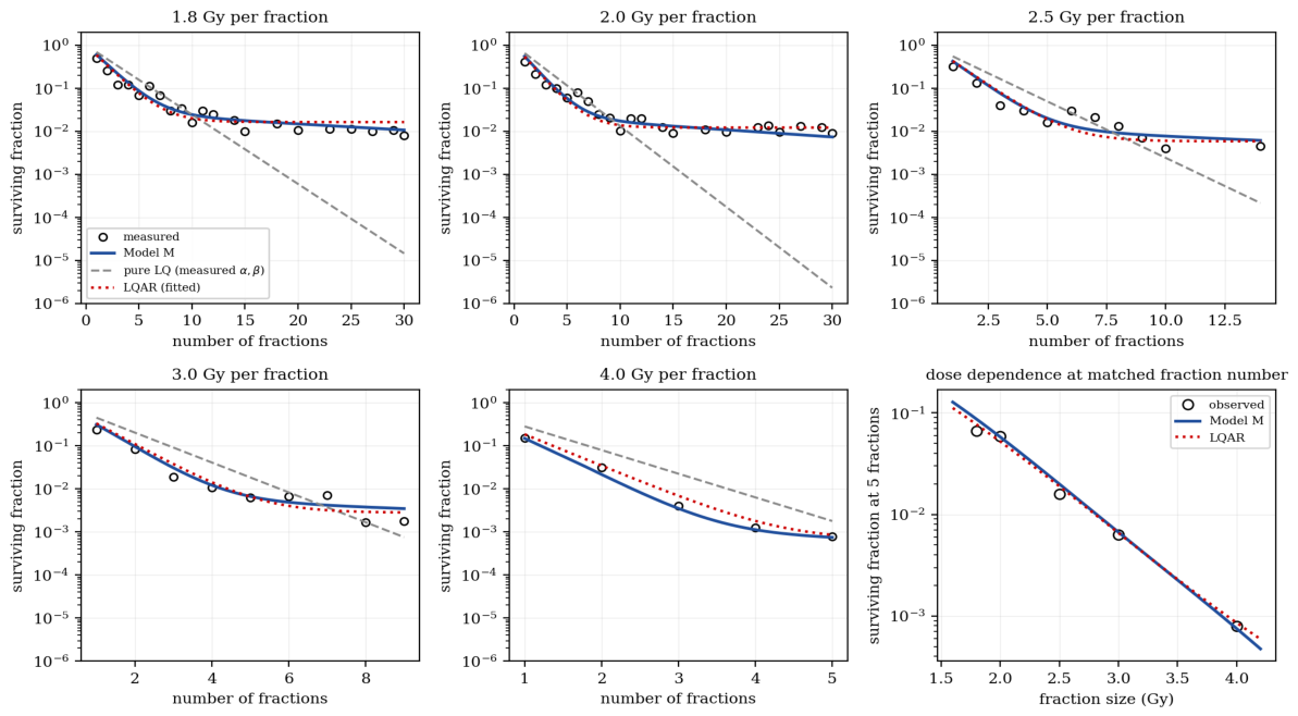
Eq. 8 identifies what that exponent is instead. Matching the local slopes of the derived and inserted floors at a reference fraction size d₀ gives ln(α/β)eff = (nw+1)(α + 2βd₀) — an effective ratio that is a joint property of the consolidation window and the radiosensitivity, not a radiosensitivity ratio. At 2 Gy this predicts 3.69 against 4.35 fitted and 2.32 measured: agreement in direction and order of magnitude but differing by fifteen per cent, recorded as partial rather than quantitative success. Third, and against the construction: with whole fraction sizes held out in turn, Model M generalises slightly worse than the expression it outperforms in sample (0.211 against 0.198). We report this as a limitation rather than a result. It is the expected signature of five parameters against two on 68 points from one experiment, and it means the fit demonstrates that the derived floor is of the right shape and magnitude, not that the mechanism is validated.
4.3. What the Fit Establishes, and What It Does Not
The consolidation window returned is nw = 1.75 fractions, 95 per cent profile-likelihood interval [1.25, 2.50] — about two and a half calendar days on a five-fraction week. It is not an artefact of the assumed radiosensitivity ratio: imposing α/β anywhere between 1.0 and 6.0 and refitting leaves the best window between 1.75 and 2.00 in every case, and it is moderately robust to curve removal. But a structural limit deserves emphasis: a single-dose-level fractionation curve cannot identify nw at all, however good the data, because the window and the write coupling trade off exactly along one curve. Multiple fraction sizes are not a refinement here but the identifiability condition — a design constraint on any experiment intended to measure the window.
Three residuals should be recorded. The model reproduces the direction of the fraction-size dependence but overshoots its magnitude, predicting a 114-fold fall between 1.8 and 4.0 Gy at five fractions against an observed 84-fold. At the last fraction measured on each curve it agrees to within +0.13, −0.10, +0.14, +0.29 and −0.03 in log₁₀. And it overpredicts survival after a single fraction by +0.08 to +0.13 in log₁₀, the residue of the assay discrepancy of Section 4.1. The window estimate also sits awkwardly against the drug analogue: Li et al. (2026) score functional adaptation at about a week of exposure and full resistance at about four weeks, where the radiation data return about two and a half days. The estimates are not in numerical agreement, and we claim only the ordering the construction requires — that the write be slower than a fraction and faster than a course. All data used here were digitised from published figures, and the analysis rests on one cell line, so none of this validates the mechanism. What it establishes is narrower and still worth having: an expression the field inserted by hand is derivable, its exponent has a structural interpretation the fitted symbol does not support, and the derived form describes the fraction-size dependence at least as well while doing far less violence to independently measured radiosensitivity.
Figure 5.
The structural results survive the specialisation. Left: order effect against tolerance ratio under the delayed write, for a twenty-fraction 40 Gy course whose fraction sizes fall linearly from 3.0 to 1.0 Gy delivered large-to-small against its exact time reverse; the effect vanishes identically at r = 1. Centre: build-up of the written compartment, showing the consolidation delay and its faster completion at larger fraction size. Right: profile likelihood in the consolidation window, giving nw = 1.75 fractions with a 95 per cent interval of [1.25, 2.50].
Figure 5.
The structural results survive the specialisation. Left: order effect against tolerance ratio under the delayed write, for a twenty-fraction 40 Gy course whose fraction sizes fall linearly from 3.0 to 1.0 Gy delivered large-to-small against its exact time reverse; the effect vanishes identically at r = 1. Centre: build-up of the written compartment, showing the consolidation delay and its faster completion at larger fraction size. Right: profile likelihood in the consolidation window, giving nw = 1.75 fractions with a 95 per cent interval of [1.25, 2.50].
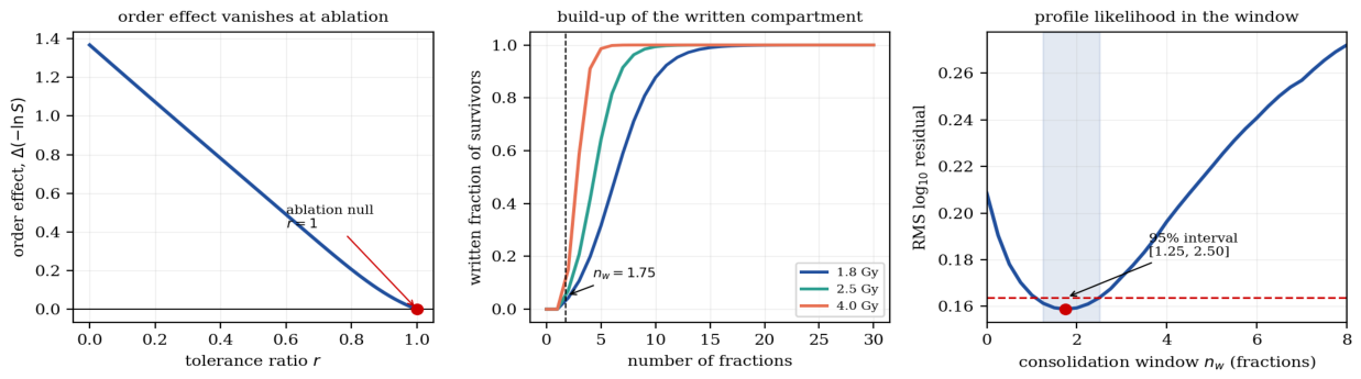
Table 5.
summarises the evidential status of the axioms, and the biological assumptions. Status: Settled (measured in irradiated tumours); Anchored (measured in the nearby drug/antibiotic field and transferred); Assumption (adopted rather than established, and stated as such); Idealisation (adopted for tractability, with the consequence of relaxing it stated); Bet (falsifiable, untested).
Table 5.
summarises the evidential status of the axioms, and the biological assumptions. Status: Settled (measured in irradiated tumours); Anchored (measured in the nearby drug/antibiotic field and transferred); Assumption (adopted rather than established, and stated as such); Idealisation (adopted for tractability, with the consequence of relaxing it stated); Bet (falsifiable, untested).
| Axioms # | Claim | Evidence / basis | Status |
|---|---|---|---|
| Axiom 1 | two differentially-killed compartments | Gu 2022; Zhao 2023; Forissier 2025 | Settled |
| Axiom 2 | one-way write; reversion frozen on course scale | Zhao 2023 (slow reversion); van den Berg 2020 (full reversal after recovery, radiation-direct) | Anchored: reversion real but slow vs course |
| Axiom 3 | multiplicative tolerance g=rh | Form untested in radiation: van den Berg 2020 fit an additive floor in survival, not a hazard modifier, and compare no forms | Assumption (sets the sign; see §4.2) |
| Axiom 4 | lagged write, τw > 0 | Li 2026 (adaptation scored at ≈1 wk; low-dose exposure confers resistance to a later high dose); van den Berg 2020 (phenotype over ≈2–3 wk); §6.5 (1.75 fx from radiation data) | Anchored; estimates differ in magnitude, agree that τw exceeds a fraction and is shorter than a course |
5. Framework Results Beyond the Core
The exact results live on a compact core: two populations, the lagged write, the tolerance gap. The full architecture earns its place not by proving the theorem but by giving it reach. The results below require layers and couplings the core does not contain, are correspondingly weaker in status, and we mark them as such.
5.1. The Consolidation-Timing Window
Consider a tolerance-writing delivery, a radiation-free gap, then a consolidative dose meeting partly reverted cells. Persister escape and regrowth during the gap produce an interior optimum in the gap length: too short and the consolidation meets a still-tolerant population, too long and regrowth has replaced what was killed. In the residual-dominated regime the optimum is logarithmic in the ratio of persister to sensitive survival at the consolidative dose, and vanishes as that gap closes. On the illustrative parameter set it is about ten days; on the clearance rate the radiation persister data support, roughly three to five weeks. We therefore report the existence of an interior optimum with two-sided fall-off as the structural claim and the location as an order-of-magnitude range. This runs through the reseeding arm, not the survival law.
5.2. Bistable, Hysteretic Escape
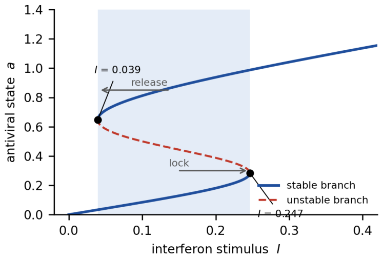
Zhao et al. (2023) report mutual repression between type-I interferon signalling and the budding programme: cells must suppress antiviral signalling to escape, and budding suppresses it in turn. This double-negative feedback reduces to a self-reinforcing variable whose fixed points form an S-curve with saddle-node folds bracketing a bistable window. As the stimulus rises the persister locks; as it falls the cells release and bud out; the two thresholds differ, so the transition is path-dependent — a signature a purely bottom-up cascade cannot produce, and one requiring the gate as a distinct variable. We demonstrate the gate’s own bistability, not the stronger claim that the closed persister–population loop creates a new attractor with an irreversible tipping point; in the present model the return coupling shifts the coexisting states only marginally. We leave the emergent form explicitly as a prediction, quantifiable with a causal-emergence measure on the loop (Pigozzi et al., 2025).
Figure 6.
The hysteretic escape gate. Antiviral state against interferon stimulus for the double-negative feedback of the A layer. Solid, stable branches; dashed, unstable; markers, saddle-node folds; shaded, the bistable window. The lock and release thresholds differ (I = 0.039 and 0.247), so the transition is path-dependent. This is the gate’s own bistability, propagated through the loop, not a new attractor created by closing it.
Figure 6.
The hysteretic escape gate. Antiviral state against interferon stimulus for the double-negative feedback of the A layer. Solid, stable branches; dashed, unstable; markers, saddle-node folds; shaded, the bistable window. The lock and release thresholds differ (I = 0.039 and 0.247), so the transition is path-dependent. This is the gate’s own bistability, propagated through the loop, not a new attractor created by closing it.
5.3. The Selection Rule Across Layers
The core says that a single schedule’s order matters and that the effect is gated by the tolerance. The architecture lifts this into a statement about which modalities interact — a lift with no formulation in a single-variable reduction. Because the redox layer (dose rate), the signal layer (spatial pattern) and the persister layer (memory, re-irradiation) are distinct, separately perturbable handles, two patterns perturbing the same variable through the same channel add, whereas two perturbing different variables interact. Order-dependence within one schedule and interaction across two modalities are thereby the same structure read in two settings, gated by the same tolerance factor, so both vanish together under ablation. The rule’s reach is at present promissory: one entry of the interaction matrix is computed and the spatial band is sketched rather than solved. The architecture earns its place as falsifiable structure for a research programme, not yet as delivered breadth.
5.4. Non-Redundancy of the Couplings
Setting each coupling to its null in turn and recomputing six behaviours — the order effect, the dose-rate law, the cross-modality interaction, the consolidation window, the hysteresis width and the reversion flux — maps the architecture at once, and the picture is sparse. As shown in the coupling ablation map below (Figure 7), the write and the tolerance back-arm are the masters of every kill-shaping behaviour: removing either collapses order, dose-rate, interaction and window together. Closing the tolerance gap sends all four to zero in one stroke while leaving reversion and hysteresis intact — the ablation null appearing as a single row. The lag governs the timing behaviours; the reseeding arm and the gate bistability each carry exactly one behaviour. No coupling is redundant. Under a ±50 per cent one-at-a-time sweep of every rate the signs of the order law and the interaction are retained in every case.
6. Delivery Modalities Under One Account
Each modality primarily perturbs an identified state variable, so whether two interact becomes a structural property of which variables they touch rather than a quantity to be screened, with LQ as the common frozen-state baseline. Conventional and altered fractionation act on the temporal axis, their effect being the schedule-dependence of Eq. 5, reducing to LQ when the persister resets between fractions. Stereotactic delivery acts on the magnitude axis, and Section 5.1 is exactly the question of when such a consolidation should follow a prior delivery. FLASH acts on the dose-rate axis through the redox layer, both depleting oxygen radiolytically (Pratx & Kapp, 2019; Vozenin et al., 2019) and potentially outrunning the induction lag. Re-irradiation engages the persister layer directly, since prior treatment has already written a state the second course meets.
Spatially fractionated radiotherapy is the one major modality the temporal core does not contain, and saying so is part of the account. Its peak–valley geometry acts on a spatial collective variable — the non-targeted signalling field (Mothersill & Seymour, 2001; Prezado et al., 2024) — which the signal layer carries non-spatially but which becomes a distinct, diffusing band when space is resolved. Promoting the signal to a reaction–diffusion field is the framework’s spatial extension (Vaitheeswaran, 2026c): the tolerant state is then written wherever the signal reaches, broader than the delivered dose, while differential survival removes it at the ablative peaks, displacing the durable, memory-bearing population into the valleys. This is consistent with the finding that response tracks valley rather than peak dose, and predicts that the geometry maximising durable memory differs from the dose-optimal one.
The selection rule then reads across modalities. FLASH and spatially fractionated delivery perturb different variables and are predicted to interact rather than add — a prediction standing against a combination literature reporting their joint use as at most additive (Schneider et al., 2022), and one a preclinical system now exists to test, spatially fractionated delivery having been realised at FLASH dose rates in vivo (Taylor et al., 2026). Two fractionation schedules, perturbing the same variable, should add. The framework thus converts combination design, in principle, from empirical screening into a structural prediction, and it commits to signs before magnitudes — which is what makes it falsifiable ahead of calibration.
7. Discussion
7.1. The Framework and the Theorem
Everything proved in Section 3 lives on three variables, so an obvious objection is that the other layers are decoration. Two answers. First, three results follow only from the wider structure: the interaction selection rule requires distinct, separately perturbable variables, and on the core there is only one handle; the consolidation window runs through the reseeding arm and the population layer; and the path-dependent escape requires the gate as an independent bistable variable. Remove the extra layers and the exact results survive, but what remains is a theorem about fractionation, not an account of radiation response. Second, the reduction of Section 2.4 derives the two-compartment core rather than assuming it. Without the timescale hierarchy a reviewer would rightly ask why radiation response should be represented by two compartments and a first-order lag rather than any other low-dimensional caricature. With it, the core is what the layered state contracts to, each symbol acquires a definition in terms of an identified process, and the domain of validity of the closed form is explicit. The architecture is what makes the theorem a result rather than a modelling choice.
7.2. What the Figures Establish, and What They Do Not
Read together the figures separate three grades of claim. Figure 1 and Figure 2 carry the structural content and contain nothing fitted: both loci are reached exactly, and at clinical scale the two orderings of a 60 Gy course in thirty fractions coincide to machine precision when the tolerance gap closes and diverge by 0.67 in −ln S when it does not. Figure 3 constrains the claim rather than supporting it, and is why Section 3.6 is worded as it is: the ablation null holds exactly for every tolerance functional, but the sign of the order effect separates them only where the gap is wide, and at the tolerance ratio the fit of Section 4 returns all three forms front-load. The keystone contrast is unaffected, because the null it tests is form-independent; what is affected is the secondary hope of reading the functional form off the sign.
Figure 4 carries most of the empirical weight and repays close reading. The gap between the grey line and the measurements — about 3.6 orders of magnitude at 2 Gy by thirty fractions — is the effect any adaptive account must explain, and it is far too large to be a calibration artefact. That the blue and red curves both track the data is the point rather than a weakness: the question is not whether an adaptive term is needed, which is settled, but whether it must be inserted or can be derived, and the two curves are close because they are describing the same real phenomenon by different routes. What separates them is not visible in the figure but in Table 4 — what each must do to independently measured radiosensitivity, and what happens when that radiosensitivity is held fixed. Nor can the figure show the held-out behaviour, where the ranking reverses. Figure 5 then checks that specialising to a fraction train has not quietly destroyed the structure: the null survives the delayed write, and the consolidation window is identified rather than assumed. Figure 6 belongs to the framework and not to the theorem, and is included for exactly that reason — it is a behaviour the two-compartment core cannot produce at all. Figure 7 shows non-redundancy of the couplings.
7.3. Repair and Redistribution, Externalised by Design
Of the classical R’s, three are represented — intrinsic radiosensitivity as the frozen LQ baseline, reoxygenation as the redox layer, repopulation as the population layer and the reseeding arm. Sublethal repair and cell-cycle redistribution are deliberately held outside. Mathematically they must be: a repair convolution violates the local-kernel axiom by putting history into the kill law itself, and an explicit cycle compartment dissolves the two-state structure and the exact nulls with it. More importantly, they are the principal competing mechanisms for the very timing-dependence the persister predicts (Curtis, 1986; Hawkins, 1994; Powathil et al., 2013; Kuznetsov & Kolobov, 2023). Holding them outside is what makes the central prediction discriminating: the claim is not that timing matters — which they already explain — but that a specific, persister-dependent component of it exists and is abolished by persister depletion, whereas the other components would survive. The omitted R’s are the controls against which the mechanism is defined.
7.4. The Planning Quantities Become History-Dependent
If response is the behaviour of a coupled state rather than a function of dose alone, planning becomes the problem of steering a state. Biologically effective dose (BED) loses its order-independence, and the difference between two schedules of equal nominal value is computed from Eq. 5 rather than fitted. Tumour-control probability (TCP), computed with a single fixed surviving fraction, over-estimates control whenever treatment induces a less sensitive compartment during the course. Complication probability is reframed, the carried-forward injury being a decaying persistent state rather than a static dose ledger — though on the normal-tissue side the persister is largely the wrong compartment, making the tumour-side correction the asymmetric one. Each quantity is recovered exactly in the frozen-state limit and departs from it precisely where LQ itself departs from observation. Because each intervention changes the state the next will face, maximising immediate kill is not generally optimal — territory adaptive therapy already occupies (Zhang et al., 2017; Gatenby & Brown, 2020), which the framework recovers through the reseeding arm rather than discovers. That each variable has its own external handle also makes the modalities the designed perturbations rendering the latent state identifiable, the interaction terms being themselves constraining observables (Raue et al., 2009). Individual parameters stay sloppy in the generic way (Gutenkunst et al., 2007; Chis et al., 2011); the carrying claims are the sign and null invariants holding across the whole unidentifiable manifold. The realistic control target is a posterior over a partially observed state updated as data accrue (Gelman et al., 2013), developed separately (Vaitheeswaran, 2026a, 2026b).
7.5. What the State Might Represent
The formal results are interpretation-free, but a state-coupled kill law makes a question well-posed that a scalar dose model cannot ask. One reading is informational: the write-and-inherit step encodes a transient insult into a durable, heritable record, the gate is a decision module, and the top-down arm is downward causation from a pattern rather than a concentration — a picture recent gene-regulatory-network work renders concrete (Pigozzi et al., 2025; Eckert et al., 2024), sitting within the thesis that life is matter plus information (Davies, 2019). A complementary agential reading treats the layers as a degraded instance of the multicellular integration that normally coordinates cells toward tissue-level goals (Levin, 2021), and the timescale ordering — cheap reversible responses before durable committed ones — recurs across biology (Ng & Kinjo, 2022; Schick et al., 2026). We hold both as framing, not claim.
7.6. Predictions
(P1) Persister-ablation kill switch — the keystone. The matched-dose, matched-fraction order effect vanishes identically when the persister is depleted, and the null it rests on is exact and form-independent. The confound is cell-cycle redistribution, which produces a matched-dose order effect the classical tradition already captures; the persister signature must therefore persist at inter-fraction gaps longer than cycle resynchronisation and be abolished specifically by persister depletion rather than by cycle perturbation. The sign is informative about the functional form of the gate, but only where the tolerance gap is wide (Figure 3), so we do not rest the design on it. Falsifier: an effect surviving persister depletion, or decaying on the cell-cycle timescale. Feasibility is not speculative: a complex-I inhibitor showed on-treatment target engagement against persisters in a phase I trial (Yap et al., 2023), persisters are selectively vulnerable to ferroptosis induction (Hangauer et al., 2017), writer inhibition abolishes the analogous written state (Li et al., 2026), inhibition of a candidate radiation writer radiosensitises schedule-dependently (Brassesco et al., 2013), and the in vivo paradigm for quantifying schedule-dependent drug–radiation interaction is established (Helbig et al., 2014).
(P2) The observable must be total clonogens, not plating efficiency. The ablation null holds exactly for the sum of sensitive and persister clonogens. It does not hold for the ratio of that sum to a total including a non-clonogenic arrested compartment, and in that ratio an artefactual order effect of the opposite sign appears. The keystone experiment must report total clonogens per flask normalised to cells seeded; run the conventional way it could return a spurious result of the wrong sign.
(P3) The effective floor exponent rises with fraction size, scaling as exp[(nw +1)(α + 2βd₀)] and predicting 3.36, 3.69, 4.69, 5.96 and 9.61 at 1.8, 2.0, 2.5, 3.0 and 4.0 Gy; falsified by per-fraction-size fits returning a constant ratio.
(P4) Cross-modality interaction: modalities perturbing different state variables interact non-additively while same-channel pairs add, the cleanest test being dose rate crossed with temporal sequence.
(P5) An interior consolidation window: a finite inter-dose delay maximises kill with two-sided fall-off, the existence being the structural claim and the location inheriting the clearance-time uncertainty over roughly ten to forty days.
(P6) Reversion to baseline: once the persister clears and progeny revert, salvage re-irradiation acts at full efficacy — a retrodiction the reversion data support.
(P7) Emergent irreversible resistance: the closed persister–population feedback may create a tipping point past which resistance persists after withdrawal; left as a prediction pending a bifurcation analysis.
7.7. Status, Limitations, and the Clinical Path
Separating what is proved, fitted and asserted: proved, on the reduced core and exactly, are the closed form, both nulls, the autonomy boundary and the fractionation specialisation with its derived floor; fitted, on one cell line from digitised figures, are the consolidation window, the write coupling and the tolerance ratio, with the qualification that the fit generalises slightly worse than the expression it outperforms in sample; asserted and still open are the functional form of the tolerance in radiation, the numerical agreement between the radiation and drug-analogue write timescales, and the interaction matrix beyond its single computed entry. Two apparent contributions do not survive scrutiny as independent results: the decomposition into timescale bands is partly a reorganisation of structure the field already holds, and reinterpreting the radiosensitivity coefficients as state-dependent adds no predictive power until the dependence is specified. Nor do we explain normal-tissue FLASH sparing, the persister being the wrong compartment for it.
The minimal model is a theorem vehicle, not a clinical predictor; outcome prediction genuinely requires all the R’s. The path is therefore not to extend it into a full-R simulation — which would destroy the closed form and re-enter a field of calibrated models — but to validate the persister mechanism in isolation via the ablation experiment and then contribute it as a single additional term to such a model, in which repair and redistribution are supplied in their established forms.
8. Conclusion
We have proposed that radiation response is the response of a single coupled state resolved into five layers ordered by relaxation time and read out through one kill kernel of which LQ is the exact frozen-state limit, and we have used the separation of those clocks to reduce the architecture to a two-compartment core on which the system is solved exactly. The resulting closed-form surviving fraction becomes independent of the entire delivery history on exactly two loci: an ablation locus, resting on a left-eigenvector identity that holds at every instant and is therefore exact, all-orders, and independent of both the tolerance functional and the write; and an instantaneous-write locus, where the write becomes proportional to the kill. Cell-autonomy of the write is precisely the condition under which a closed form exists, and the ablation null survives even where it does not. Specialized to a fraction train under a delayed write, the same equation derives a survival floor the field had inserted into LQ by hand, and identifies its exponent as a property of the consolidation window rather than the radiosensitivity ratio its notation asserts — a reinterpretation the data support, since the inserted floor overpredicts observed survival by an order of magnitude when held to the radiosensitivity measured in the same cells. The wider architecture is what turns that theorem into an account: it supplies the reduction that derives the core rather than assuming it, the distinct perturbable variables that make the interaction rule statable, the reseeding arm that produces a consolidation window, and the escape gate that produces path-dependence — none of which the core contains. Read across modalities it places FLASH, spatially fractionated, stereotactic and conventional delivery under one account in which interaction follows from which variables a pair perturbs. The construction remains uncalibrated where it matters most, and its clinical content is funnelled through one decisive experiment: a matched-dose, order-reversed contrast, read out as total clonogens, with and without persister depletion.
References
- Abbott, K., Hardo, G., Li, R., Bradley, J., Zarkan, A., & Bakshi, S. (2026). Stress History Establishes a Transient Tolerant State That Shapes Antibiotic Survival Upon Resuscitation. Advanced Science, e21993. [CrossRef]
- Ahmed, K. A., Correa, C. R., Dilling, T. J., et al. (2014). Altered fractionation schedules in radiation treatment: A review. Seminars in Oncology, 41(6), 730–750. [CrossRef]
- Alfonso, J. C. L., & Berk, L. (2019). Modeling the effect of intratumoral heterogeneity of radiosensitivity on tumor response over the course of fractionated radiation therapy. Radiation Oncology, 14, 88. [CrossRef]
- Almquist, K. J., & Banks, H. T. (1976). A theoretical and computational method for determining optimal treatment schedules in fractionated radiation therapy. Mathematical Biosciences, 29(1–2), 159–179. [CrossRef]
- Ayati, B. P., Kapitanov, G. I., & Loew, L. M. (2016). A mathematical modeling framework for the combined effects of radiotherapy and chemotherapy. arXiv:1603.00349.
- Belli, M., & Tabocchini, M. A. (2020). Ionizing radiation-induced epigenetic modifications and their relevance to radiation protection. International Journal of Molecular Sciences, 21(17), 5993. [CrossRef]
- Bergonié, J., & Tribondeau, L. (1906). Interprétation de quelques résultats de la radiothérapie et essai de fixation d’une technique rationnelle. Comptes Rendus des Séances de l’Académie des Sciences, 143, 983–985. [Translation: Radiation Research, 11(4), 587–588, 1959.].
- Blanes, S., Casas, F., Oteo, J. A., & Ros, J. (2009). The Magnus expansion and some of its applications. Physics Reports, 470(5–6), 151–238.
- Bortfeld, T., Ramakrishnan, J., Tsitsiklis, J. N., & Unkelbach, J. (2015). Optimization of radiation therapy fractionation schedules in the presence of tumor repopulation. INFORMS Journal on Computing, 27(4), 788–803. [CrossRef]
- Brassesco, M. S., Roberto, G. M., Morales, A. G., et al. (2013). Inhibition of NF-κB by dehydroxymethylepoxyquinomicin suppresses invasion and synergistically potentiates temozolomide and γ-radiation cytotoxicity in glioblastoma cells. Chemotherapy Research and Practice, 2013, 593020. [CrossRef]
- Brenner, D. J. (2008). The linear-quadratic model is an appropriate methodology for determining isoeffective doses at large doses per fraction. Seminars in Radiation Oncology, 18(4), 234–239. [CrossRef]
- Chis, O.-T., Banga, J. R., & Balsa-Canto, E. (2011). Structural identifiability of systems biology models: A critical comparison of methods. PLoS ONE, 6(11), e27755. [CrossRef]
- Curtis, S. B. (1986). Lethal and potentially lethal lesions induced by radiation — a unified repair model. Radiation Research, 106(2), 252–270. [CrossRef]
- Davern, M., Turner, C. J., Griffin, D., Bencsics, L., Chan, B. C., Kung, J. Y. T.,... & Letai, A. (2025). Drug-tolerant persisters and immunotherapy persister cells exhibit cross-resistance and share common survival mechanisms. Cell Death & Differentiation, 1-18. [CrossRef]
- Davies, P. C. W. (2019). The Demon in the Machine: How Hidden Webs of Information Are Solving the Mystery of Life. University of Chicago Press.
- Dayanc, B., et al. (2025). AP-1 as a targetable mediator of acquired resistance to osimertinib in EGFR-mutant lung cancer. Cell Death & Disease. [CrossRef]
- Di Dio, C., Porrazzo, A., De Gregorio, A., Morciano, P., Tabocchini, M. A., Cenci, G.,... & Esposito, G. (2025). In vivo study of the radioadaptive response and low-dose hyper-radiosensitivity for chromosome breaks induced by gamma rays in wild-type Drosophila melanogaster larval neuroblasts: Dose and dose rate dependence. PLoS One, 20(6), e0325608. [CrossRef]
- Eckert, L., Vidal-Saez, M. S., Zhao, Z., et al. (2024). Habituation as an emergent property of a biochemical feedback network. Current Biology, 34(24), 5646–5658.
- Enderling, H., Chaplain, M. A. J., & Hahnfeldt, P. (2010). Quantitative modeling of tumor dynamics and radiotherapy. Acta Biotheoretica, 58(4), 341–353. [CrossRef]
- Foray, N. (2012). Victor Despeignes (1866–1937): How a hygienist became the first radiation oncologist. Cancer Radiothérapie, 17(3), 244–254. [On the law of Bergonié and Tribondeau.].
- Forissier, V., Rivera-Franco, M. M., Cabeza-Segura, M., et al. (2025). The LRP4/YAP axis drives the radiation-tolerant persister cell state in breast cancer. Theranostics, 15(15), 7528–7546.
- Fowler, J. F. (1989). The linear-quadratic formula and progress in fractionated radiotherapy. British Journal of Radiology, 62(740), 679–694. [CrossRef]
- Fu, A., Kim, H., Chetty, I. J., et al. (2026). Optimal radiotherapy dose scheduling with variable fraction sizes and treatment breaks via sequential convex programming. Physics and Imaging in Radiation Oncology, 39, 101003.
- Gatenby, R. A., & Brown, J. S. (2020). Integrating evolutionary dynamics into cancer therapy. Nature Reviews Clinical Oncology, 17(11), 675–686. [CrossRef]
- Gelman, A., Carlin, J. B., Stern, H. S., et al. (2013). Bayesian Data Analysis (3rd ed.). Chapman and Hall/CRC.
- Gillies, R. J., Verduzco, D., & Gatenby, R. A. (2012). Evolutionary dynamics of carcinogenesis and why targeted therapy does not work. Nature Reviews Cancer, 12(7), 487–493. [CrossRef]
- Gouw, Z. A. R., Jasperse, B., Sonke, J.-J., et al. (2024). Early treatment response assessment during radiotherapy and its use for adaptive fractionation. Radiotherapy and Oncology, 190, 110006.
- Gray, L. H., Conger, A. D., Ebert, M., et al. (1953). The concentration of oxygen dissolved in tissues at the time of irradiation as a factor in radiotherapy. British Journal of Radiology, 26(312), 638–648. [CrossRef]
- Gu, J., Mu, N., Jia, B., et al. (2022). Targeting radiation-tolerant persister cells as a strategy for inhibiting radioresistance and recurrence in glioblastoma. Neuro-Oncology, 24(7), 1056–1070. [CrossRef]
- Gutenkunst, R. N., Waterfall, J. J., Casey, F. P., et al. (2007). Universally sloppy parameter sensitivities in systems biology models. PLoS Computational Biology, 3(10), e189. [CrossRef]
- Hall, E. J., & Giaccia, A. J. (2018). Radiobiology for the Radiologist (8th ed.). Wolters Kluwer.
- Hangauer, M. J., Viswanathan, V. S., Ryan, M. J., Bole, D., Eaton, J. K., Matov, A., Galeas, J., Dhruv, H. D., Berens, M. E., Schreiber, S. L., McCormick, F., & Bassik, M. C. (2017). Drug-tolerant persister cancer cells are vulnerable to GPX4 inhibition. Nature, 551(7679), 247–250. [CrossRef]
- Hawkins, R. B. (1994). A statistical theory of cell killing by radiation of varying linear energy transfer. Radiation Research, 140(3), 366–374. [CrossRef]
- Helbig, L., Koi, L., Brüchner, K., et al. (2014). Hypoxia-inducible factor pathway inhibition resolves tumor hypoxia and improves local tumor control after single-dose irradiation. International Journal of Radiation Oncology, Biology, Physics, 88(1), 159–166. [CrossRef]
- Joiner, M. C., Marples, B., Lambin, P., et al. (2001). Low-dose hypersensitivity: Current status and possible mechanisms. International Journal of Radiation Oncology, Biology, Physics, 49(2), 379–389. [CrossRef]
- Kallman, R. F. (1972). The phenomenon of reoxygenation and its implications for fractionated radiotherapy. Radiology, 105(1), 135–142. [CrossRef]
- Krasowska, J., Kłos, J., Ostrowski, J., & Fornalski, K. W. (2026). Understanding the Radiation Adaptive Response: General Methodology and Theoretical Approaches to the Study of the Radioadaptation Phenomenon. Dose-Response, 24(2), 15593258261442577. [CrossRef]
- Kuznetsov, M., & Kolobov, A. (2023). Optimization of antitumor radiotherapy fractionation via mathematical modeling with account of 4 R’s of radiobiology. Journal of Theoretical Biology, 558, 111371. [CrossRef]
- Levin, M. (2021). Bioelectric signaling: Reprogrammable circuits underlying embryogenesis, regeneration, and cancer. Cell, 184(8), 1971–1989. [CrossRef]
- Lewin, T. D., Maini, P. K., Moros, E. G., Enderling, H., & Byrne, H. M. (2018). The evolution of tumour composition during fractionated radiotherapy: implications for outcome. Bulletin of Mathematical Biology, 80(5), 1207–1235. [CrossRef]
- Li, J., Ravindran, P. T., O’Farrell, A., Busch, G. T., Boe, R. H., Niu, Z.,... & Raj, A. (2026). AP-1 mediates cellular adaptation and memory formation. Nature Communications. [CrossRef]
- Ling, H. H., Huang, H. Y., Huang, C. M., Yasir, M., Ko, C. C., Yadav, V. K.,... & Tsai, J. T. (2026). Drug-tolerant persister cells in head and neck squamous cell carcinoma: Molecular mechanisms and therapeutic opportunities. Translational Oncology, 63, 102579. [CrossRef]
- Magnus, W. (1954). On the exponential solution of differential equations for a linear operator. Communications on Pure and Applied Mathematics, 7(4), 649–673. [CrossRef]
- McMahon, S. J. (2019). The linear quadratic model: Usage, interpretation and challenges. Physics in Medicine & Biology, 64(1), 01TR01. [CrossRef]
- Mothersill, C., & Seymour, C. (2001). Radiation-induced bystander effects: Past history and future directions. Radiation Research, 155(6), 759–767. [CrossRef]
- Ng, E. T. H., & Kinjo, A. R. (2022). Computational modeling of plasticity-led evolution. arXiv:2209.05599. [CrossRef]
- Olivieri, G., Bodycote, J., & Wolff, S. (1984). Adaptive response of human lymphocytes to low concentrations of radioactive thymidine. Science, 223(4636), 594–597. [CrossRef]
- Pajonk, F., Vlashi, E., & McBride, W. H. (2010). Radiation resistance of cancer stem cells: the 4 R’s of radiobiology revisited. Stem Cells, 28(4), 639–648. [CrossRef]
- Park, C., Papiez, L., Zhang, S., et al. (2008). Universal survival curve and single fraction equivalent dose: Useful tools in understanding potency of ablative radiotherapy. International Journal of Radiation Oncology, Biology, Physics, 70(3), 847–852. [CrossRef]
- Pigozzi, F., Goldstein, A., & Levin, M. (2025). Associative conditioning in gene regulatory network models increases integrative causal emergence. Communications Biology, 8(1), 1027. [CrossRef]
- Powathil, G. G., Adamson, D. J. A., & Chaplain, M. A. J. (2013). Towards predicting the response of a solid tumour to chemotherapy and radiotherapy treatments: Clinical insights from a computational model. PLoS Computational Biology, 9(7), e1003120. [CrossRef]
- Pratx, G., & Kapp, D. S. (2019). A computational model of radiolytic oxygen depletion during FLASH irradiation and its effect on the oxygen enhancement ratio. Physics in Medicine & Biology, 64(18), 185005. [CrossRef]
- Prezado, Y., Grams, M., Jouglar, E., et al. (2024). Spatially fractionated radiation therapy: A critical review on current status of clinical and preclinical studies and knowledge gaps. Physics in Medicine & Biology, 69(10), 10TR02. [CrossRef]
- Raue, A., Kreutz, C., Maiwald, T., et al. (2009). Structural and practical identifiability analysis of partially observed dynamical models by exploiting the profile likelihood. Bioinformatics, 25(15), 1923–1929. [CrossRef]
- Russo, M., Chen, M., Mariella, E., Peng, H., Rehman, S. K., Sancho, E.,... & Bardelli, A. (2024). Cancer drug-tolerant persister cells: from biological questions to clinical opportunities. Nature Reviews Cancer, 24(10), 694-717. [CrossRef]
- Scheidegger, S., Fuchs, H. U., Zaugg, K., et al. (2013). Using state variables to model the response of tumour cells to radiation and heat: A novel multi-hit-repair approach. Computational and Mathematical Methods in Medicine, 2013, 587543. [CrossRef]
- Schick, L., Eichenlaub, E., Drexel, F., Mayer, A., Chen, S., Roper, M., & Alim, K. (2026). Decision-making in light-trapped slime molds involves active mechanical processes. PRX Life, 4(2), 023026. [CrossRef]
- Schneider, T., Fernandez-Palomo, C., Bertho, A., et al. (2022). Combining FLASH and spatially fractionated radiation therapy: The best of both worlds. Radiotherapy and Oncology, 175, 169–177. [CrossRef]
- Scott, B. R. (2004). A biological-based model that links genomic instability, bystander effects, and adaptive response. Mutation Research, 568(1), 129–143. [CrossRef]
- Sharma, S. V., Lee, D. Y., Li, B., et al. (2010). A chromatin-mediated reversible drug-tolerant state in cancer cell subpopulations. Cell, 141(1), 69–80. [CrossRef]
- Sinclair, W. K., & Morton, R. A. (1966). X-ray sensitivity during the cell generation cycle of cultured Chinese hamster cells. Radiation Research, 29(3), 450–474. [CrossRef]
- Taylor, E. R. J. F., Ruan, J.-L., Paillas, S., Tullis, I. D. C., Higgins, G. S., & Petersson, K. (2026). A preclinical setup for spatially fractionated radiation therapy with electrons. Medical Physics. [CrossRef]
- Vaitheeswaran, R. (2026a). The Ghost in the Cancer: Towards a new science of radiation oncology. Notion Press.
- Vaitheeswaran, R. (2026b). On the observability and structural identifiability of the coupled adaptive-state radiobiology model. Preprints. [CrossRef]
- Vaitheeswaran, R. (2026c). Extending the Kinetic-Bystander Model for Spatially Fractionated Radiotherapy with Intracellular Epigenetic Memory. Preprints. [CrossRef]
- Valcz, G., Gatenby, R. A., Újvári, B., Buzás, E. I., & Molnár, B. (2025). Adaptive cancer therapy: can non-genetic factors become its achilles heel?. Oncogene, 44(42), 3999-4005. [CrossRef]
- Van den Berg, J., Castricum, K. C. M., Meel, M. H., et al. (2020). Development of transient radioresistance during fractionated irradiation in vitro. Radiotherapy and Oncology, 148, 107–114. [CrossRef]
- Vozenin, M.-C., Hendry, J. H., & Limoli, C. L. (2019). Biological benefits of ultra-high dose rate FLASH radiotherapy: Sleeping beauty awoken. Clinical Oncology, 31(7), 407–415. [CrossRef]
- Wang, S., Lei, J., Zou, X., & Jin, S. (2025). Integrating multiscale mathematical modeling and multidimensional data reveals the effects of epigenetic instability on acquired drug resistance in cancer. PLOS Computational Biology, 21(2), e1012815. [CrossRef]
- Wei, J., & Norman, E. (1963). Lie algebraic solution of linear differential equations. Journal of Mathematical Physics, 4(4), 575–581.
- Wolff, S. (1998). The adaptive response in radiobiology: Evolving insights and implications. Environmental Health Perspectives, 106(Suppl 1), 277–283. [CrossRef]
- Yap, T. A., Daver, N., Mahendra, M., Zhang, J., Kamiya-Matsuoka, C., Meric-Bernstam, F., Konopleva, M., et al. (2023). Complex I inhibitor of oxidative phosphorylation in advanced solid tumors and acute myeloid leukemia: phase I trials. Nature Medicine, 29(1), 115–126. [CrossRef]
- Yu, V. Y., Nguyen, D., Pajonk, F., et al. (2015). Incorporating cancer stem cells in radiation therapy treatment response modeling and the implication in glioblastoma multiforme treatment resistance. International Journal of Radiation Oncology, Biology, Physics, 91(4), 866–875. [CrossRef]
- Zhang, J., Cunningham, J. J., Brown, J. S., & Gatenby, R. A. (2017). Integrating evolutionary dynamics into treatment of metastatic castrate-resistant prostate cancer. Nature Communications, 8, 1816. [CrossRef]
- Zhao, Y., Li, D., Zhou, Y., et al. (2023). Cancer cells enter an adaptive persistence to survive radiotherapy and repopulate the tumor. Advanced Science, 10(8), 2204177.
Figure 7.
Coupling-ablation map. Each cell gives the fraction of a behaviour retained when a coupling is removed (1 = intact, 0 = abolished). The write (κ) and the tolerance back-arm (r) govern every kill-shaping behaviour; the (1 − r) theorem appears as the tolerance row; the reseeding arm and the escape-gate bistability each carry a single behaviour. No coupling is redundant.
Figure 7.
Coupling-ablation map. Each cell gives the fraction of a behaviour retained when a coupling is removed (1 = intact, 0 = abolished). The write (κ) and the tolerance back-arm (r) govern every kill-shaping behaviour; the (1 − r) theorem appears as the tolerance row; the reseeding arm and the escape-gate bistability each carry a single behaviour. No coupling is redundant.
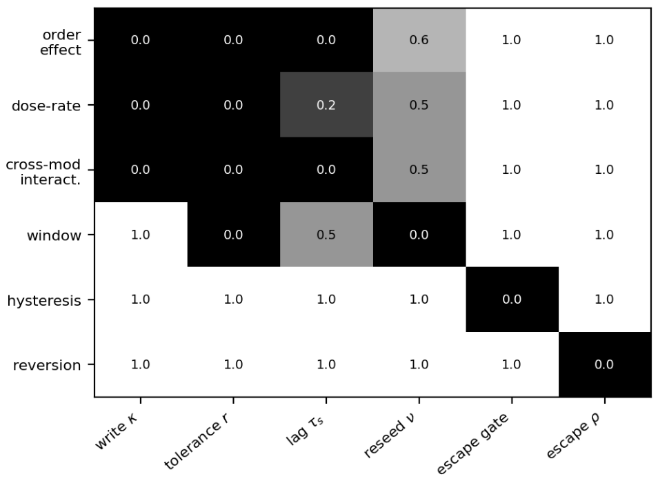
Table 1.
The five layers, ordered by relaxation timescale, with the biological process and experimental literature grounding each. The M layer spans radiolytic chemistry (milliseconds to seconds, the FLASH channel) up to oxygen replenishment (minutes). The escape gate A relaxes faster than the persister state it controls and is slaved to its bistable steady state.
Table 1.
The five layers, ordered by relaxation timescale, with the biological process and experimental literature grounding each. The M layer spans radiolytic chemistry (milliseconds to seconds, the FLASH channel) up to oxygen replenishment (minutes). The escape gate A relaxes faster than the persister state it controls and is slaved to its bistable steady state.
| Layer | Var. | Timescale | Biological process | Key references |
|---|---|---|---|---|
| M — redox | x | ms–seconds | radical chemistry; radiolytic oxygen depletion; oxygen enhancement; FLASH oxygen dynamics | Gray et al. 1953; Pratx & Kapp 2019; Vozenin et al. 2019 |
| S — stress signal | s | minutes–hours | DNA-damage and stress signalling; non-targeted (bystander) collective signal | Curtis 1986; Hawkins 1994; Mothersill & Seymour 2001 |
| A — escape gate | a | hours–days | type-I interferon / budding toggle releasing persister progeny | Zhao et al. 2023 |
| B — persister | Np, b | days–weeks | reversible tolerant persister state; write-and-inherit; conserved across tumour types | Gu 2022; Zhao 2023; Forissier 2025; Li 2026 |
| E — population | Ns, Np | weeks–months | clonal evolution under selection; repopulation; adaptive therapy | Gatenby & Brown 2020; Enderling et al. 2010 |
Disclaimer/Publisher’s Note: The statements, opinions and data contained in all publications are solely those of the individual author(s) and contributor(s) and not of MDPI and/or the editor(s). MDPI and/or the editor(s) disclaim responsibility for any injury to people or property resulting from any ideas, methods, instructions or products referred to in the content. |
© 2026 by the authors. Licensee MDPI, Basel, Switzerland. This article is an open access article distributed under the terms and conditions of the Creative Commons Attribution (CC BY) license (http://creativecommons.org/licenses/by/4.0/).
Copyright: This open access article is published under a Creative Commons CC BY 4.0 license, which permit the free download, distribution, and reuse, provided that the author and preprint are cited in any reuse.