

Submitted:
08 June 2026
Posted:
09 June 2026
You are already at the latest version
Abstract
Raman spectroscopy combined with machine learning offers a rapid, label-free approach for bacterial identification, but robust translation remains challenged by spectral variability, biological heterogeneity, and limited model interpretability. Here, we present an integrated evaluation of an optimized Spectral Transformer (ST) framework for Raman-based bacterial classification benchmarked against a systematically optimized one-dimensional convolutional neural network (1D-CNN). The comparison was performed using a curated 36-class dataset comprising 15 Gram-negative bacterial entries, 15 Gram-positive bacterial entries, one non-bacterial microorganism, and five background/reference classes, enabling evaluation of both species-level and fine-grained bacterial classification. Under 15 dB noise-augmented evaluation, the ST achieved 80.6% ± 0.3% accuracy and a Matthews correlation coefficient (MCC) of 0.801 ± 0.003, outperforming the 1D-CNN baseline with 72.9% ± 0.3% accuracy andanMCCof0.721±0.003. Integrated Gradients analysis combined with attention map visualization enabled multi-level model interpretation, revealing that the ST’s improved robustness correlates with more bounded attribution patterns during misclassification, whereas the 1D-CNN’s feature attribution becomes scattered under noise perturbation. Importantly, this interpretability-driven analysis identified model-specific failure modes in the baseline architecture, including an over-reliance on non-specific spectral regions under noise, which can inform future data collection strategies and guide refinements to experimental protocols. These results demonstrate that attention-based spectral modeling improves Raman-based bacterial classification under noise-perturbed conditions while enabling multi-level interpretability that bridges model understanding with actionable feedback on experimental design and data quality requirements.
Keywords:
raman spectroscopy
; bacterial identification
; spectral transformer
; machine learning
; deep learning
; chemometrics
; chemical fingerprinting
; integrated gradients
; attention maps
; model interpretability
; 1d-cnn
; noise robustness
; microbial classification
; spectral preprocessing
; raman-based diagnostics
1. Introduction
Raman spectroscopy (RS) is a label-free and non-invasive optical technique that provides molecularly specific information through inelastic photon scattering. By probing intrinsic vibrational fingerprints, RS enables rapid chemical and biochemical characterization without cultivation, staining, or external labeling [1,2,3,4]. Its high chemical specificity and minimal sample preparation requirements have established RS as a promising platform for biomedical diagnostics, microbiological identification, environmental monitoring, and materials characterization [5,6,7,8,9,10]. However, Raman spectra are high-dimensional and often affected by overlapping vibrational bands, weak signal intensity, fluorescence background, baseline drift, and instrument-dependent distortions. These factors complicate interpretation and limit direct translation into robust analytical workflows. Machine learning (ML) has therefore become a key component in Raman analysis, enabling automated feature extraction, classification, denoising, and decision support [11,12,13,14,15,16,17,18,19]. ML has substantially advanced Raman-based bacterial identification. Classical approaches such as PCA–LDA [20,21], support vector machines (SVMs), k-nearest neighbors (kNN) [22,23], and random forests [24] perform well on small and controlled datasets but often fail in distinguishing closely related species and under realistic biological and instrumental variability. Deep-learning methods address these limitations by learning nonlinear spectral representations directly from data. Convolutional and residual networks capture local spectral features [12,25], recurrent models exploit sequential structure, and autoencoders enable denoising and dimensionality reduction [26,27]. More recently, transformer-based models have shown strong potential due to their ability to capture long-range dependencies between non-adjacent spectral features using self-attention [13,15,28].
Despite significant advances in Raman spectroscopy combined with machine learning, robust deployment for bacterial diagnostics remains limited by domain shift, spectral variability, and insufficient model interpretability. Classification performance obtained under controlled conditions often decreases when spectra are acquired across different instruments, laboratories, sample-preparation protocols, or biological backgrounds [12,13,18,29]. Reliable Raman–ML translation therefore requires models that are robust to noise, background variation, instrument-dependent spectral distortions, and heterogeneous sample conditions, while also providing uncertainty-aware and interpretable predictions [30,31]. Consequently, large, diverse, and well-annotated spectral datasets are essential to develop transferable Raman-based microbial diagnostics [32,33].
In this work, we present an integrated evaluation of an optimized ST framework for Raman-based bacterial identification and benchmark it against a systematically optimized 1D-CNN. The comparison is performed on a heterogeneous curated 36-class Raman dataset comprising 15 Gram-negative bacterial entries, 15 Gram-positive bacterial entries, one non-bacterial microorganism, and five background/reference classes acquired under diverse experimental conditions. The dataset includes species-, strain-, phenotype-, instrument-, and medium-associated subclasses, including reference and clinical isolate entries of E. coli as well as methicillin-susceptible and methicillin-resistant S. aureus. This enables evaluation of both species-level classification and discrimination between closely related bacterial subclasses. Building on our previous hyperspectral Raman framework [13], the optimized ST is assessed in terms of predictive performance, robustness to controlled noise perturbations, prediction variability, and model interpretability. Monte Carlo dropout and bootstrap resampling are used to estimate empirical prediction and performance variability [34]. Furthermore, the internal decision matrix of the ST is directly visualized using 2D spectral attention maps to uncover distinct functional attention archetypes. To complement this architecture-specific analysis, class-wise Integrated Gradients are applied to representative spectra to provide an algorithm-agnostic comparison of feature attributions between the two models [35]. These attribution profiles are quantified using the Gini coefficient and spectral attribution spread along the Raman-shift axis. The study therefore evaluates attention-based spectral modelling as a robust and interpretable chemometric framework for Raman-based bacterial classification, while recognizing that further external validation will be required to assess applicability to clinical infection diagnostics and antimicrobial-resistance-related screening.
2. Methods
Raman spectra were acquired using two complementary platforms: the DFM hyperspectral Raman microscope and the Lightnovo spectrometer. The dual-platform dataset was used to increase spectral heterogeneity and to assess whether the preprocessing and spectral-alignment workflow could accommodate instrument-dependent variability. The systems differ in excitation wavelength, spectral range, sampling density, spectral resolution, detector response, and background characteristics, thereby broadening the experimental variability represented in the dataset. This analysis was intended as a practical robustness and data-alignment test, rather than a complete calibration-transfer or instrument-transfer-function study.
2.1. The Raman Platforms
Two complementary Raman platforms were used to compile the spectral database and assess the robustness of the model across measurement conditions. The first platform was a custom-built hyperspectral Raman microscope equipped with a 785 nm diode laser operated at 60 mW [13]. A schematic overview of the measurement workflow is shown in Figure 1. The excitation beam was spatially filtered through a single-mode fiber to obtain a stable near-Gaussian profile and focused onto bacterial samples on substrates using a long-working-distance 100× objective with NA ≈ 0.85. Automated hyperspectral mapping was performed using a motorized XYZ stage with positioning precision of approximately 200 nm. The backscattered Raman light was separated by an 800 nm dichroic mirror, spectrally filtered, and coupled into an HR320 spectrometer equipped with a cooled CCD detector. The microscope spectra covered 700–1600 with 480 spectral points and an effective spectral resolution of approximately 10 using a 1 s integration time per pixel. The second platform was a commercial Lightnovo Raman spectrometer operated with 830 nm excitation. In this study, Lightnovo spectra comprised 2356 sampled points over 50–2400 with an effective spectral resolution of approximately 8 . The two platforms were included to expose the machine-learning workflow to spectra acquired under different instrumental conditions. The aim was not to perform a dedicated calibration-transfer study, but to evaluate the robustness of the classification pipeline across complementary Raman measurement systems.
2.2. Raman Spectral Databases for Machine Learning
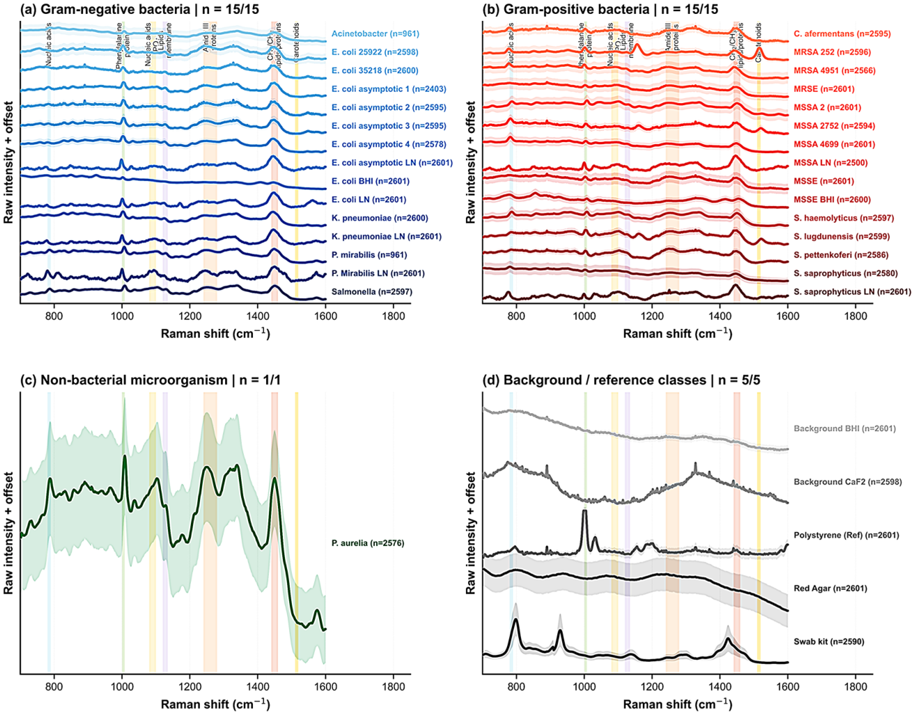
Reliable ML-assisted Raman spectroscopy requires curated datasets that capture both biological diversity and experimental variability [30,36]. In the 700–1600 fingerprint region, bacterial Raman spectra contain overlapping contributions from nucleic acids, proteins, lipids, carbohydrates, cell-wall components, and, where present, carotenoid pigments. Important spectral regions include nucleic-acid-associated bands near 780–790 and 1080–1100 , protein-related features around 1004, 1240–1280 and 1440–1460 , lipid and membrane contributions near 1120–1135 and 1440–1460 , and carotenoid bands around 1155 and 1515 [37]. These overlapping biochemical signatures form a distributed Raman fingerprint, motivating models capable of integrating weak bands, relative intensity patterns and subtle spectral-shape variations across the full spectral window. Spectral variability can arise from species- and strain-level differences, growth conditions, sample handling, biological background and instrument response. If such variability is insufficiently represented, models may overfit to dataset-specific features and generalize poorly under deployment conditions. We therefore constructed a 36-class curated Raman database comprising 15 Gram-negative bacterial entries, 15 Gram-positive bacterial entries, one non-bacterial microorganism and five background/reference classes acquired under heterogeneous experimental conditions (Figure A2) together with an overview of the data set is provided in Figure A1.
All Raman spectra were processed using a harmonized workflow implemented in ramanspy [16], following the sequence shown in Figure 1. (1) Defective pixels, artefactual spectra, and acquisition-related outliers were first removed. (2) The spectra were then aligned to a common Raman-shift axis, resolution-matched where required, and interpolated to a shared 700–1600 fingerprint-region grid. (3) Cosmic-spike removal was subsequently applied, followed by (4) Savitzky–Golay denoising using an 11–15 point window and a second- or third-order polynomial. (5) Baseline correction was performed using iarPLS with a second-order smoothness penalty and iterative convergence until stabilization of the baseline estimate. (6) Finally, all spectra were vector-normalized prior to machine-learning analysis. The DFM dataset consisted exclusively of experimentally acquired spectra, whereas the Lightnovo dataset typically contained 50–100 experimental spectra per class and was supplemented with synthetic spectra generated by noise-aware augmentation, including additive noise, intensity fluctuations, and baseline perturbations. This approach improved statistical robustness and reduced class imbalance while preserving experimentally realistic spectral variability. The final balanced dataset contained approximately 2600 spectra per class and was split into mutually exclusive training, validation, and test sets using a 70:15:15 partition. To minimize data leakage, the train/validation/test partitioning was performed before augmentation at the level of the original experimental spectra or acquisition files, and all augmented spectra derived from a given original measurement were retained within the same split.
2.3. Robustness Testing under Noise-Augmented Raman Conditions
To assess robustness under more realistic acquisition conditions, additive white Gaussian noise (AWGN) was introduced at the acquisition-file level. Noise augmentation was used as a controlled stress test rather than a direct model of a specific spectrometer. Based on empirical SNR scaling, the applied noise level approximately corresponds to a reduction in integration time from 1 s to the sub-0.1 s regime, although the exact equivalence varies between spectral features. This approach applies a common noise floor to all spectra within a file, approximating fixed hardware-related thermal and readout noise from a given spectrometer setting. For each file containing a spectral matrix , where N is the number of spectra and M is the number of spectral points, the global signal power was estimated as:
For a target signal-to-noise ratio of 15 dB, the corresponding noise power was calculated as:
Gaussian noise with standard deviation was then sampled independently and added to each spectral intensity value:
This procedure generated noise-perturbed spectra with a controlled 15 dB noise level while preserving file-specific spectral structure.
2.4. Model Design, Optimization
We implemented an attention-based deep-learning architecture, the ST, adapting our previous hyperspectral Raman framework for bacterial classification [13]. To establish a robust deep-learning benchmark, we concurrently evaluated an optimized one-dimensional convolutional neural network (1D-CNN) baseline [11,12]. The hyperparameters for both the ST and the 1D-CNN were jointly optimized over 100 Optuna trials using the Tree-structured Parzen Estimator algorithm, with cross-entropy validation serving as the optimization objective [38]. The complete optimization procedure and parameter search grids for both architectures are detailed in the Appendix under the section Hyperparameter Optimization Search Space.
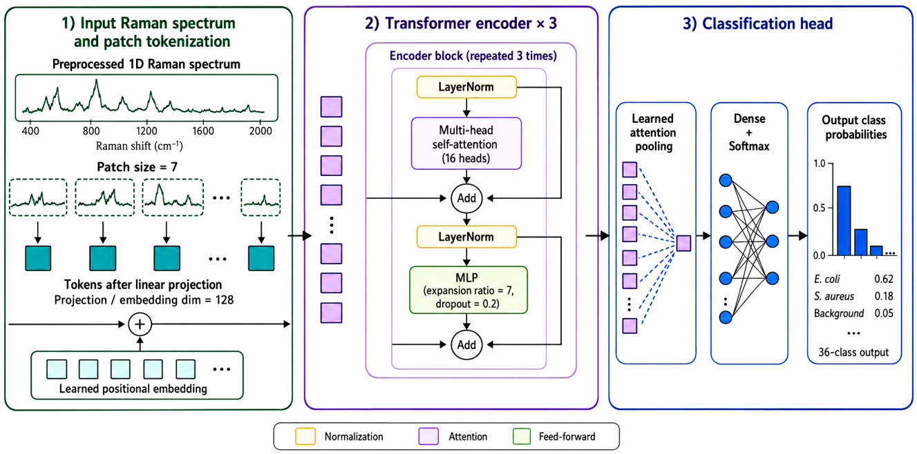
The ST goes beyond localized convolutional kernels by utilizing global attention mechanisms to model long-range dependencies across the spectral continuum. This framework provides sensitivity to narrow Raman bands while retaining the capacity to model multivariate biochemical fingerprint patterns, which is critical for both broad-category classification and fine-grained discrimination between closely related bacterial classes under heterogeneous and cross-instrument conditions. Hyperparameter optimization identified a moderately deep and expressive ST architecture as optimal for Raman classification under noise-augmented evaluation. One-dimensional Raman spectra are processed using a patch size of 7 and mapped into a latent feature space with a projection embedding dimension of 128. The network employs three Transformer encoder blocks, each comprising 16 parallel attention heads, layer normalization before each sublayer, and Gaussian Error Linear Unit (GELU) multi-layer perceptrons with an expansion ratio of 7. Overfitting was mitigated using a dropout probability of 0.2. Instead of rigid flattening, a learned attention-pooling mechanism aggregates the spectral-token representations according to their informational relevance prior to final softmax classification. The ST was trained for 60 epochs using the Adam optimizer, a batch size of 64, and an optimized learning rate of .
Similarly, the optimized 1D-CNN provides a strong discriminative baseline by hierarchically extracting localized spectral features, Raman band shapes, and short- to intermediate-range spectral patterns. The architecture consists of three sequential convolutional blocks with progressively increasing filter capacities of 64, 128, and 256. Each block utilizes a kernel size of 11 with a stride of 1, zero padding, ReLU activation, and spatial dropout, followed by spatial downsampling via max-pooling with a window size and stride of 2. Following convolutional feature extraction, the learned representations are aggregated using global average pooling and mapped through a fully connected layer of 128 dense units. Notably, the network was trained without weight decay, relying strictly on the aforementioned spatial dropout and a standard dropout probability of 0.13 in the dense layer for regularization. The baseline model was trained for 60 epochs using sparse categorical cross-entropy loss and the Adam optimizer, operating with a batch size of 256 and an optimized learning rate of .
Figure 2.
ST-based workflow for Raman classification and attention-based interpretation. (a) ST architecture for Raman-based bacterial classification. A preprocessed 1D Raman spectrum is divided into spectral patches of length 7, projected into 128-dimensional token embeddings, combined with learned positional embeddings, and processed by three Transformer encoder blocks with 16-head self-attention. The encoded token sequence is aggregated using learned attention pooling and classified by a dense softmax layer to generate probabilities across the 36 classes.
Figure 2.
ST-based workflow for Raman classification and attention-based interpretation. (a) ST architecture for Raman-based bacterial classification. A preprocessed 1D Raman spectrum is divided into spectral patches of length 7, projected into 128-dimensional token embeddings, combined with learned positional embeddings, and processed by three Transformer encoder blocks with 16-head self-attention. The encoded token sequence is aggregated using learned attention pooling and classified by a dense softmax layer to generate probabilities across the 36 classes.
2.5. Extraction of Spectral Attention Matrices
To interpret the internal decision-making process of the ST, we extracted the self-attention weights from the final encoder block. Each attention head possesses an associated weight (W), representing its relative importance in the final classification decision. To quantify the functional role of each head, we calculated the Spectral Correlation Profile across the 800– Raman shift. This was achieved by measuring the Pearson correlation coefficient () between the individual attention head weights and the class-averaged physical reference spectra from the evaluation dataset. This metric provides a quantitative basis for categorizing the functional mechanisms of the attention heads independent of their raw mathematical weights.
2.6. Explainable AI via Integrated Gradients
Finally, to demystify both networks and ground their predictions in structural reality, eXplainable AI (XAI) was implemented via Integrated Gradients [35,39]. Crucially, because the baseline 1D-CNN architecture does not possess an inherent self-attention mechanism, direct structural comparison using internal weight layers is restricted to the ST framework. Integrated Gradients resolves this asymmetry by serving as a unified, model-agnostic feature attribution method, allowing the distinct decision-making strategies of both models to be directly cross-examined.
This approach computes the path integral of the gradients along a straight-line trajectory from a reference baseline spectrum to the actual input spectrum x. To ensure chemically meaningful attributions rather than artifactual noise, the dataset grand average spectrum was utilized as the baseline rather than a zero-filled array. The continuous integral was computationally approximated using a Riemann sum over 50 discrete linear interpolation steps (). The feature attribution for the i-th spectral channel is mathematically defined as:
where represents the model’s predicted probability for the target class. By tracking these attributions across the spectral continuum, we directly mapped the specific Raman shifts () governing complex target discrimination. Rather than relying on subjective visual interpretation of these feature maps, the resulting attribution distributions were subsequently quantified using information-theoretic metrics to objectively evaluate the structural differences in feature utilization between the 1D-CNN and the ST.
2.7. Prediction Variability and Bootstrap Evaluation
To quantify the predictive uncertainty and assess the structural robustness of the models, we implemented a combined Monte Carlo (MC) Dropout and non-parametric bootstrapping framework. Following the approach of Gal and Ghahramani [34], MC Dropout was enabled at test time to serve as an efficient approximation of Bayesian inference. Because the evaluated models possess fundamentally different topologies, the architectural application of MC Dropout was explicitly tailored to each framework. For the 1D-CNN, the dropout probability p was optimized dynamically via Bayesian hyperparameter optimization (Optuna) within a bounded search space of p .
To capture the uncertainty of the model throughout the network hierarchy, 1D Spatial Dropout was applied after the convolutional blocks, while standard Dropout was reserved for fully connected layers [40]. Dropping entire feature maps via Spatial Dropout is critical, as it prevents the network from bypassing stochasticity and outputting artificially low uncertainty by relying on the local spatial correlations of neighboring features. In contrast, for the PyTorch-based ST, a fixed dropout rate (p=0.2) was maintained to preserve sequence representation stability, with stochastic path dropout applied inherently within the multi-head self-attention matrices and dense feed-forward blocks. To execute MC Dropout across both the PyTorch and TensorFlow/Keras frameworks, the default evaluation routines of the respective libraries were programmatically overridden to keep all dropout layers active during inference, ensuring that each forward pass utilized a uniquely sampled network architecture.
Concurrently, non-parametric bootstrapping was applied to the evaluation dataset to establish robust empirical confidence intervals for our population-level metrics (Accuracy, MCC). To capture both model uncertainty and finite-sample evaluation variance simultaneously, we executed exactly N=200 combined stochastic evaluation iterations for both models. For each of the 200 iterations, a full stochastic forward pass was executed. In tandem, a bootstrap sample—drawn with replacement—was generated from the test set indices. Performance metrics were computed by evaluating the MC-perturbed predictions strictly against the ground-truth labels of this resampled subset. While MC Dropout yields an uncalibrated relative measure of confidence rather than absolute probabilities, aggregating these 200 paired stochastic iterations provides a highly conservative estimation of the models’ reliability across both architectural weight variance and finite-sample distribution shifts.
3. Results
3.1. Classification Performance under Noise Augmentation
High classification accuracy in curated Raman datasets should be interpreted in the context of the similarity between training, validation, and test distributions. Although the present dataset (Figure A2) includes heterogeneous measurements, standardized preprocessing, spectral harmonization, and augmentation reduce unwanted experimental variability and improve class separability. Under these controlled conditions, the ST and 1D-CNN achieved accuracies of approximately 99% and 97%, respectively. However, such performance may overestimate deployment accuracy in clinical or environmental samples, where spectra may contain mixed microbial populations, biological background, matrix effects, weak bacterial signals, and instrument-dependent domain shifts. To bridge the gap between these idealized laboratory measurements and the noisy realities of field deployment, we systematically evaluated the robustness of both models using the targeted noise augmentation framework detailed in the Methods section. By deliberately degrading the signal-to-noise ratio (SNR) to a challenging 15 dB, our objective was to simulate the diminished spectral quality inherent to complex measurement environments.
The confusion matrices and localized sub-matrix analyses for the optimized 1D-CNN and ST are shown in Figure 3(a) and Figure 4(a), respectively. Under the 15 dB noise-augmented evaluation framework, the ST achieved an overall accuracy of and an MCC of . In comparison, the optimized 1D-CNN baseline achieved an overall accuracy of and an MCC of . When predictive uncertainty was quantified via the combined Monte Carlo (MC) dropout and bootstrapping framework, the models exhibited slight performance degradations consistent with stochastic inference. The 1D-CNN experienced an MCC drop of 0.014 (to ) and an accuracy reduction to . The ST experienced a smaller MCC degradation of 0.005 (to ) and an accuracy reduction to . While the absolute performance drop is larger for the 1D-CNN, this disparity must be interpreted within the context of their distinct Bayesian approximations. As detailed in the Methods, the 1D-CNN was subjected to 1D Spatial Dropout, an aggressive perturbation that drops entire convolutional feature maps, whereas the ST utilized standard sequence-based path dropout. Consequently, while these asymmetric dropout methods preclude a direct comparison of the performance drops, the perturbed ST still maintains an absolute classification performance well above the unperturbed 1D-CNN baseline.
To gain deeper insight into the models’ predictive behavior, we evaluated the localized accuracy within highly similar sub-groups, specifically Staphylococcus species variants and E. coli strains (Figure 3b–c and Figure 4b–c). The ST model demonstrated a notable increase in MCC over the 1D-CNN for the Staphylococcus variants, while maintaining an E. coli classification performance within of the 1D-CNN baseline. This highlights that in highly multiplexed datasets, global performance metrics can obscure more nuanced, localized classification dynamics among closely related sub-classes, underscoring the need for robust model interpretability.
Although quantitative performance metrics reveal differences in classification accuracy and robustness between the models, they do not explain how the underlying spectral representations drive individual predictions. We therefore performed a multi-level interpretation of the ST model using 2D spectral attention maps, complemented by Integrated Gradients for model-agnostic attribution analysis. This combined interpretability framework links predictive performance to specific Raman fingerprint regions and model failure modes, providing insight into how spectral information is used under noise-perturbed conditions and how future data acquisition, preprocessing, and model optimization strategies may be refined.
3.2. Mechanistic Interpretation of Spectral Attention
Figure 5 illustrates the mechanistic interpretation of the ST’s internal decision matrix using polystyrene as a reference material. To decode the model’s inner workings, we calculated the Spectral Correlation Profile across the 800– Raman shift. Each attention head possesses an associated weight (W), representing its relative importance in the final classification decision. By measuring the Pearson correlation coefficient () between individual head weights and the class-averaged physical reference spectrum, we identified three distinct functional attention archetypes.
The first archetype, termed Biomarker Detectors (Figure 5a), exhibits a strong positive correlation, exemplified by Head 13 (, ). These heads autonomously identify physical vibrational bands by locking onto primary emission and absorption Raman shifts to confirm target presence, closely mimicking the analytical approach of an experienced spectroscopist. Conversely, Inhibitory Attention Mechanisms (Figure 5b) operate via a negative correlation framework. Exemplified by Head 9 (, ), these heads actively highlight contrasting regions, focusing on the absence of features and mapping empty window spaces to suppress out-of-class spectral profiles. Finally, Structural Context Heads (Figure 5c) display near-zero correlation with the mean spectrum, as seen in Head 11 (, ). Rather than isolating specific chemical peaks, they map global baseline geometry, distributing weight along local matrix diagonals to calculate peak widths, baseline curvatures, and instrument noise thresholds independent of raw peak intensity.
Ultimately, the network aggregates these independent sub-decisions into a final hidden layer, visualized as the Model Consensus Integrated Layer (Figure 5d) (, ). This integrated profile represents the mathematically weighted linear summation of all active attention heads across the transformer framework. Notably, all four panels exhibit vertical bands corresponding to the model’s attention to relative intensity ratios between specific features and the global spectral structure. Rather than relying on a single spectral feature, the consensus map demonstrates how the system blends absolute biomarker tracking, inhibitory background validation, and local geometric context to establish a highly transparent, physics-aligned decision boundary.
3.3. Explainable AI via Integrated Gradients
To differentiate between 1D-CNN and ST, we employed an algorithm-agnostic Integrated Gradients (IG). By mapping attribution scores back to the original Raman shifts, IG allows us to identify the specific biomolecular features driving the classifications, ensuring the models rely on genuine physical vibrational bands rather than artifactual noise.
For all IG calculations, the grand average of the entire dataset was utilized as the baseline, ensuring that the resulting attribution scores highlight the specific vibrational features distinguishing a given prediction from the global mean spectrum. To quantify the topology of these attributions, we evaluated two key spatial metrics. The Gini Coefficient was utilized to measure the sparsity or concentration of the attribution weights, where a higher value indicates reliance on a few sharp peaks [41]. Simultaneously, the Spatial Spread was calculated as the spatial variance (second moment) of the attribution density along the wavenumber axis, providing a quantitative measure of how widely the network’s attention is dispersed [42].
Globally, the architectures display distinct attribution behaviors. While both models exhibit similar baseline sparsity on true positive predictions (mean Gini coefficients of 0.62 for the 1D-CNN and 0.66 for the ST), the 1D-CNN demonstrates a notably higher global Spatial Spread during failure modes. When misclassifying data, the 1D-CNN’s mean Spatial Spread expands to 315.8 (compared to 272.4 for the ST), indicating that the convolutional network’s feature extraction scatters erratically upon failure, whereas the ST’s attention remains structurally bounded.
These dynamics are further illustrated in the class-specific profiles for Staphylococcus variants and E. coli strains. On the MSSA 4699 phenotype, ST vastly outperforms 1D-CNN with a true positive ratio of 83.0% compared to CNN’s 60.7%. Although both models correctly anchor strong positive attributions on the dominant nucleic-acid-associated vibrational band near 780– (Figure 6 a–b), the ST demonstrates a fundamentally more distributed system-level allocation of feature importance across secondary diagnostic shoulders. Under failure modes (Figure 6c–d), the 1D-CNN demonstrates an over-reliance within the 1400– region, which is dominated by and bending modes characteristic of lipid and protein backbones. This disproportionate focus renders the model susceptible to common baseline and intensity fluctuations, which are erroneously interpreted as high-confidence diagnostic features. This reliance is further evidenced by a highly scattered spatial spread (318.7), highlighting the model’s vulnerability to non-specific spectral noise. In contrast, the ST’s misclassified footprint exhibits a tighter spatial spread (272.6), indicating its failure mechanism is governed by global ratio shifts rather than feature corruption.
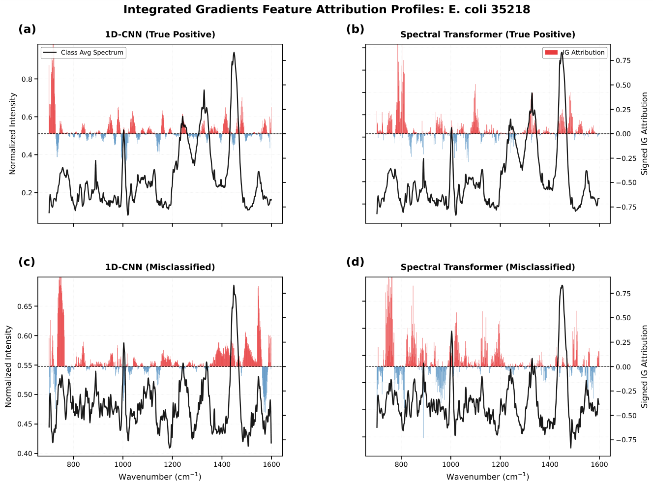
Interestingly, this localized feature extraction occasionally benefits the 1D-CNN. For the E. coli 35218 strain (Figure 7a–b), the 1D-CNN resolves a higher true positive ratio (61.1%) than the ST (54.3%). However, the failure modes for this strain (Figure 7c–d) replicate the CNN’s characteristic vulnerability: an expansion in spatial spread (335.4) as it over-indexes heavily on the 1400– lipid/amide peak window. The ST, by contrast, demonstrates a tighter failure pattern (spread 269.6) characterized by discrete attribution spikes scattered between 700 and , showing that its misclassifications are more likely triggered by subtle, non-local ratiometric perturbations.
4. Discussion
The ST achieved improved accuracy under noise-augmented evaluation (80.6% vs. 72.9% for the 1D-CNN), suggesting that attention-based architectures are more robust to spectral perturbations in this setting. The Integrated Gradients analysis (detailed in Results) reveals that this robustness correlates with qualitatively different failure mechanisms. While both architectures identify the same dominant spectral features under correct classification, they diverge in their response to noise: the 1D-CNN exhibits scattered, widespread attributions during misclassification, whereas the ST’s attention patterns remain more spatially constrained. This behavioral difference suggests that the ST’s improved noise robustness may relate to more bounded failure modes rather than fundamentally different feature utilization.
A key advantage of the ST architecture is its reliance on self-attention mechanisms, which directly provide attention maps that can be visualized and analyzed without additional post-hoc interpretation tools. Combined with model-agnostic attribution methods such as Integrated Gradients, this enables a multi-level understanding of model behavior. The IG analysis provides spectral feature importance independent of the architecture, while attention maps offer architecture-specific insights into feature relationships and weighting strategies. This layered interpretability approach permits deeper investigation of model decision-making and facilitates feedback to experimental design. Specifically, the observation that the 1D-CNN exhibits erratic attribution patterns under noise—over-relying on non-specific regions such as the 1400– lipid/amide bands—directly informs requirements for improved signal-to-noise ratios during data acquisition. Such insights can guide future data collection protocols toward experimental conditions that strengthen the signal of discriminative spectral features while minimizing artifacts that are spuriously correlated with class labels. These interpretability findings also reveal potential weaknesses in the training data distribution and preprocessing pipelines that could be remedied.
It should be noted that the ST’s superior performance is not universal across all species. The case-specific variations observed in the class-wise analysis indicate that architectural advantage depends on the spectral characteristics and signal-to-noise properties of the target class. Attribution patterns reflect architectural properties and their interaction with the training data; they do not constitute direct biochemical evidence for specific molecular assignments. These observations are specific to the present dataset and preprocessing conditions. Several factors limit confident extrapolation of these findings to clinical or cross-laboratory settings. Raman spectra are sensitive to biological heterogeneity, sample preparation, optical alignment, spectral resolution, and instrument-specific transfer functions. These sources of variation introduce domain shifts that exceed the scope of standard preprocessing. High performance within this curated evaluation does not establish universal cross-platform robustness or clinical readiness. Reliable deployment will require systematic validation across independent instruments, laboratories, and acquisition protocols. The findings support attention-based models as a viable approach for Raman spectral classification, with interpretable failure modes that merit further investigation. Monte Carlo dropout and bootstrap resampling provide estimates of variability but should not be treated as calibrated uncertainty measures without validation. Future work should include uncertainty calibration, external validation on independent datasets, and domain adaptation strategies to assess transferability across instruments.
5. Conclusions
This study benchmarked an optimized ST against an optimized 1D-CNN baseline for Raman-based bacterial identification across a heterogeneous 36-class dataset comprising bacterial species, strain/phenotype-associated subclasses, one non-bacterial microorganism, and background/reference materials. Under controlled 15 dB noise-augmented evaluation, the ST outperformed the 1D-CNN in overall classification accuracy and MCC, supporting the potential of attention-based spectral modelling for more robust Raman-based chemical fingerprint classification.
Beyond predictive performance, the combination of 2D spectral attention maps and model-agnostic Integrated Gradients enabled a multi-level interpretation of model behaviour. The results indicate that both architectures use chemically relevant Raman fingerprint regions during correct classification, but exhibit different failure modes under noise perturbation. In particular, the 1D-CNN showed more spatially scattered attributions and stronger sensitivity to non-specific spectral regions, whereas the ST maintained more bounded attribution patterns during misclassification. These findings suggest that the improved robustness of the ST may arise from more stable spectral-context modelling rather than from fundamentally different feature selection.
The study therefore supports interpretable attention-based deep learning as a promising chemometric framework for Raman spectral classification, with relevance to rapid, label-free microbial identification and broader spectroscopic chemical analysis workflows. At the same time, the results remain specific to the present dataset, preprocessing pipeline, and controlled noise-augmentation protocol. Generalization to independent instruments, laboratories, sample matrices, and real-world diagnostic or monitoring settings will require systematic external validation. Future work should therefore focus on cross-instrument testing, domain adaptation, uncertainty calibration, and iterative refinement of both experimental protocols and model architectures guided by interpretability analysis.
Author Contributions
Conceptualization, Y.M. and M.L.; methodology, Y.M., H.A., K.S. and M.L.; software, Y.M., J.B.C. and M.L.; validation, Y.M. and M.L.; formal analysis, Y.M. and M.L.; investigation, Y.M., C.T., D.K., D.R.T., K.S. and M.L.; resources, D.K., O.I., T.E.A., H.A., K.S. and M.L.; data curation, Y.M. and M.L.; writing—original draft preparation, Y.M. and M.L.; writing—review and editing, all authors; visualization, Y.M. and M.L.; supervision, H.A. and M.L.; project administration, M.L.; funding acquisition, T.E.A., O.I. and M.L. All authors have read and agreed to the published version of the manuscript.
Funding
This research was funded by the Danish Agency for Higher Education and Science and by Innovation Fund Denmark (IFD) through the Eurostars project MbSENS, case number 3109-00021B, Eurostars project MbCARE, case number 5352-00112B, and Grand Solutions project nanorRaman case number 5360-00009B.
Institutional Review Board Statement
Not applicable.
Data Availability Statement
The data and software supporting the findings of this study are not publicly available but are available from the corresponding author upon reasonable request.
Acknowledgments
The authors gratefully acknowledge Benjamin L. Thomsen for valuable scientific discussions and for developing the initial version of the Spectral Transformer architecture, which provided the foundation for the present work. During the preparation of this manuscript, ChatGPT (OpenAI) was used solely for language editing, including improving fluency, correcting grammar, and identifying typographical errors. The authors critically reviewed and edited all AI-assisted text and take full responsibility for the scientific content and final version of this publication.
Conflicts of Interest
The authors declare no conflicts of interest.
Abbreviations
The following abbreviations are used in this manuscript:
| 1D-CNN | One-dimensional convolutional neural network |
| AI | Artificial intelligence |
| AWGN | Additive white Gaussian noise |
| BHI | Brain Heart Infusion |
| CCD | Charge-coupled device |
| CNN | Convolutional neural network |
| DFM | Danish Fundamental Metrology |
| GELU | Gaussian Error Linear Unit |
| IG | Integrated Gradients |
| kNN | k-nearest neighbors |
| MCC | Matthews correlation coefficient |
| MC dropout | Monte Carlo dropout |
| ML | Machine learning |
| MRSA | Methicillin-resistant Staphylococcus aureus |
| MRSE | Methicillin-resistant Staphylococcus epidermidis |
| MSSA | Methicillin-susceptible Staphylococcus aureus |
| MSSE | Methicillin-susceptible Staphylococcus epidermidis |
| NA | Numerical aperture |
| PCA–LDA | Principal component analysis–linear discriminant analysis |
| RS | Raman spectroscopy |
| SNR | Signal-to-noise ratio |
| ST | Spectral Transformer |
| SVM | Support vector machine |
| TPE | Tree-structured Parzen Estimator |
| XAI | Explainable artificial intelligence |
Appendix A. Hyperparameter Optimization Search Space
To ensure fair evaluation, both ST and CNN architectures were systematically optimized using the Optuna hyperparameter optimization framework. For the Spectral Transformer, the search space included the learning rate ( to , log-uniform), batch size (32, 64, 128), transformer depth (1 to 3 layers), number of attention heads (4, 8, 16), token patch size (3, 5, 7, 9), MLP expansion ratio (2 to 8), and dropout probability (0.05 to 0.30). Similarly, for the 1D-CNN baseline, the search space encompassed the learning rate ( to , log-uniform), batch size (256, 512, 1024), convolutional kernel size (3, 5, 7, 9, 11), and spatial dropout probability (0.10 to 0.40). For both models, the objective function was set to minimize the validation loss over a dedicated validation fold. A Tree-structured Parzen Estimator (TPE) sampler was utilized to efficiently explore the parameter spaces across 100 independent trials, identifying the configurations that best mitigated overfitting while maximizing spectral feature extraction.
Appendix B
Figure A1 presents the class annotation table used in this study, including the assigned class labels, corresponding biological or material identities, and class categories. The dataset comprises Gram-negative bacteria, Gram-positive bacteria, one non-bacterial microorganism, and background/reference materials. Figure A2 shows the representative Raman spectra for all 36 classes included in the dataset. Together, these figures provide both the spectral overview and the taxonomic/material annotation framework used for the Raman–machine learning analysis. All bacterial samples were provided by the Department of Clinical Microbiology, Odense University Hospital, either as clinical isolates or from their biobank.
Figure A1.
Overview of the 36-class Raman spectral dataset used for machine-learning-based bacterial identification. The panel summarizes the class labels, full biological or material identity, and assigned class type, including Gram-negative bacteria, Gram-positive bacteria, one non-bacterial microorganism, and background/reference classes.
Figure A1.
Overview of the 36-class Raman spectral dataset used for machine-learning-based bacterial identification. The panel summarizes the class labels, full biological or material identity, and assigned class type, including Gram-negative bacteria, Gram-positive bacteria, one non-bacterial microorganism, and background/reference classes.
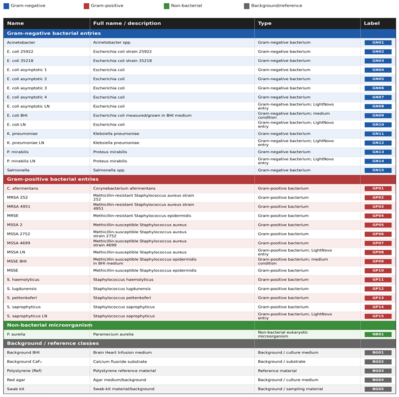
Figure A2.
Raw Raman spectral overview of the curated 36-class dataset used for machine-learning-based bacterial identification. Class-mean spectra are shown for (a) 15 Gram-negative bacterial entries, (b) 15 Gram-positive bacterial entries, (c) one non-bacterial microorganism, and (d) five background/reference classes. Each trace represents the raw mean spectrum for one class, with the shaded region indicating ±1 standard deviation across spectra within that class. For visualization only, spectra were robustly scaled and vertically offset. The numbers in parentheses indicate the number of spectra included for each class. Semi-transparent vertical bands mark representative Raman fingerprint regions associated with nucleic acids, phenylalanine/protein, phosphate/nucleic-acid vibrations, lipid and membrane contributions, amide III/proteins, deformation modes from lipids and proteins, and carotenoid-associated bands.
Figure A2.
Raw Raman spectral overview of the curated 36-class dataset used for machine-learning-based bacterial identification. Class-mean spectra are shown for (a) 15 Gram-negative bacterial entries, (b) 15 Gram-positive bacterial entries, (c) one non-bacterial microorganism, and (d) five background/reference classes. Each trace represents the raw mean spectrum for one class, with the shaded region indicating ±1 standard deviation across spectra within that class. For visualization only, spectra were robustly scaled and vertically offset. The numbers in parentheses indicate the number of spectra included for each class. Semi-transparent vertical bands mark representative Raman fingerprint regions associated with nucleic acids, phenylalanine/protein, phosphate/nucleic-acid vibrations, lipid and membrane contributions, amide III/proteins, deformation modes from lipids and proteins, and carotenoid-associated bands.
References
- Shipp, D.W.; Sinjab, F.; Notingher, I. Raman spectroscopy: techniques and applications in the life sciences. Adv. Opt. Photonics 2017, 9, 315–428. [Google Scholar] [CrossRef]
- Kerdoncuff, H.; Lassen, M.; Petersen, J.C. Continuous-wave coherent Raman spectroscopy for improving the accuracy of Raman shifts. Opt. Lett. 2019, 44, 5057–5060. [Google Scholar] [CrossRef] [PubMed]
- Ilchenko, O.; Pilhun, Y.; Kutsyk, A.; Slobodianiuk, D.; Goksel, Y.; Dumont, E.; Vaut, L.; Mazzoni, C.; Morelli, L.; Boisen, S.; et al. Optics miniaturization strategy for demanding Raman spectroscopy applications. Nat. Commun. 2024, 15, 3049. [Google Scholar] [CrossRef]
- Salbreiter, M.; Wagenhaus, A.; Rösch, P.; Popp, J. Raman spectroscopy as a comprehensive tool for profiling endospore-forming bacteria. Analyst 2025, 150, 1652–1661. [Google Scholar] [CrossRef] [PubMed]
- Ilchenko, O.; Pilgun, Y.; Kutsyk, A.; Bachmann, F.; Slipets, R.; Todeschini, M.; Okeyo, P.O.; Poulsen, H.F.; Boisen, A. Fast and quantitative 2D and 3D orientation mapping using Raman microscopy. Nat. Commun. 2019, 10, 5555. [Google Scholar] [CrossRef] [PubMed]
- Orlando, A.; Franceschini, F.; Muscas, C.; Pidkova, S.; Bartoli, M.; Rovere, M.; Tagliaferro, A. A comprehensive review on Raman spectroscopy applications. Chemosensors 2021, 9, 262. [Google Scholar] [CrossRef]
- Lee, K.S.; Landry, Z.; Pereira, F.C.; Wagner, M.; Berry, D.; Huang, W.E.; Taylor, G.T.; Kneipp, J.; Popp, J.; Zhang, M.; et al. Raman microspectroscopy for microbiology. Nat. Rev. Methods Prim. 2021, 1, 80. [Google Scholar] [CrossRef]
- Cui, D.; Kong, L.; Wang, Y.; Zhu, Y.; Zhang, C. In situ identification of environmental microorganisms with Raman spectroscopy. Environ. Sci. Ecotechnology 2022, 11, 100187. [Google Scholar] [CrossRef]
- Khristoforova, Y.; Bratchenko, L.; Bratchenko, I. Raman-based techniques in medical applications for diagnostic tasks: a review. Int. J. Mol. Sci. 2023, 24, 15605. [Google Scholar] [CrossRef]
- Akatev, D.; Meng, Y.; Brewer, J.; Chekhova, M.; Andersen, U.L.; Lassen, M. Broadly tunable quantum-enhanced Raman microscopy for advancing bioimaging. Opt. Quantum 2026, 4, 108–113. [Google Scholar] [CrossRef]
- Liu, J.; Osadchy, M.; Ashton, L.; Foster, M.; Solomon, C.J.; Gibson, S.J. Deep convolutional neural networks for Raman spectrum recognition: a unified solution. Analyst 2017, 142, 4067–4074. [Google Scholar] [CrossRef]
- Ho, C.; Jean, N.; Hogan, C.e.a. Rapid identification of pathogenic bacteria using Raman spectroscopy and deep learning. Nat. Commun. 2019, 10, 4927. [Google Scholar] [CrossRef]
- Thomsen, B.L.; Christensen, J.B.; Rodenko, O.; Usenov, I.; Grønnemose, R.B.; Andersen, T.E.; Lassen, M. Accurate and fast identification of minimally prepared bacteria phenotypes using Raman spectroscopy assisted by machine learning. Sci. Rep. 2022, 12, 16436. [Google Scholar] [CrossRef]
- Qi, Y.; Hu, D.; Jiang, Y.; Wu, Z.; Zheng, M.; Chen, Y.P. Recent Progresses in Machine Learning Assisted Raman Spectroscopy. Adv. Opt. Mater. 2023, 11. [Google Scholar] [CrossRef]
- Koyun, O.C.; et al. RamanFormer: A Transformer-Based Quantification Approach for Raman Spectroscopy. ACS Omega 2024. [Google Scholar] [CrossRef] [PubMed]
- Georgiev, D.; Pedersen, S.V.; Xie, R.; Fernández-Galiana, Á.; Stevens, M.M.; Barahona, M. RamanSPy: An open-source Python package for integrative Raman spectroscopy data analysis. Anal. Chem. 2024, 96, 8492–8500. [Google Scholar] [CrossRef] [PubMed]
- Ogunlade, B.; Tadesse, L.F.; Li, H.; Vu, N.; Banaei, N.; Barczak, A.K.; Saleh, A.A.; Prakash, M.; Dionne, J.A. Rapid, antibiotic incubation-free determination of tuberculosis drug resistance using machine learning and Raman spectroscopy. Proc. Natl. Acad. Sci. 2024, 121, e2315670121. [Google Scholar] [CrossRef] [PubMed]
- Liu, Y.; Wu, Y.; Wang, J.; Qi, J.; Zhou, C.; Xue, Y. Recent Advances in Raman Spectral Classification with Machine Learning. Sensors 2026, 26, 341. [Google Scholar] [CrossRef]
- Guo, S.; Frempong, S.B.; Salbreiter, M.; Wagenhaus, A.; Rösch, P.; Popp, J.; Bocklitz, T. Graph Neural Network in Raman Spectroscopy to Leverage the Performance and Interpretability of the Classification. Chemistry-Methods 2026, 6, e70119. [Google Scholar] [CrossRef]
- Barzan, G.; Sacco, A.; Mandrile, L.; Giovannozzi, A.M.; Portesi, C.; Rossi, A.M. Hyperspectral Chemical Imaging of Single Bacterial Cell Structure by Raman Spectroscopy and Machine Learning. Appl. Sci. 2021, 11. [Google Scholar] [CrossRef]
- Yan, S.; Wang, S.; Qiu, J.; Li, M.; Li, D.; Xu, D.; Li, D.; Liu, Q. Raman spectroscopy combined with machine learning for rapid detection of food-borne pathogens at the single-cell level. Talanta 2021, 226, 122195. [Google Scholar] [CrossRef]
- Tang, J.W.; Li, J.Q.; Yin, X.C.; Xu, W.W.; Pan, Y.C.; Liu, Q.H.; Gu, B.; Zhang, X.; Wang, L. Rapid discrimination of clinically important pathogens through machine learning analysis of surface enhanced Raman spectra. Front. Microbiol. 2022, 13, 843417. [Google Scholar] [CrossRef]
- Hu, H.; Wang, J.; Yi, X.; Lin, K.; Meng, S.; Zhang, X.; Jiang, C.; Tang, Y.; Wang, M.; He, J.; et al. Stain-free Gram staining classification of pathogens via single-cell Raman spectroscopy combined with machine learning. Anal. Methods 2022, 14, 4014–4020. [Google Scholar] [CrossRef]
- Zhang, W.; Giang, C.M.; Cai, Q.; Badie, B.; Sheng, J.; Li, C. Using random forest for brain tissue identification by Raman spectroscopy. Mach. Learn. Sci. Technol. 2023, 4, 045053. [Google Scholar] [CrossRef]
- Ralbovsky, N.M.; Lednev, I.K. Towards development of a novel universal medical diagnostic method: Raman spectroscopy and machine learning. Chem. Soc. Rev. 2020, 49, 7428–7453. [Google Scholar] [CrossRef] [PubMed]
- Junjuri, R.; Saghi, A.; Lensu, L.; Vartiainen, E.M. Evaluating different deep learning models for efficient extraction of Raman signals from CARS spectra. Phys. Chem. Chem. Phys. 2023, 25, 16340–16353. [Google Scholar] [CrossRef]
- Han, M.; Dang, Y.; Han, J. Denoising and baseline correction methods for Raman spectroscopy based on convolutional autoencoder: a unified solution. Sensors 2024, 24, 3161. [Google Scholar] [CrossRef]
- Vaswani, A.; Shazeer, N.; Parmar, N.; Uszkoreit, J.; Jones, L.; Gomez, A.N.; Kaiser, Ł.; Polosukhin, I. Attention is all you need. Adv. Neural Inf. Process. Syst. 2017, 30. [Google Scholar]
- Sakib, M.; Sayem, F.R.; Hassan, M.; Yang, Y.; Chowdhury, M.E.H.; Zughaier, S.M.; Bensaali, F.; Zhao, Y. Deep learning-based cross-device standardization of surface-enhanced Raman spectroscopy for enhanced bacterial recognition. Spectrochim. Acta Part A Mol. Biomol. Spectrosc. 2026, 347, 126931. [Google Scholar] [CrossRef]
- Lee, K.S.; Landry, Z.; Athar, A.; Alcolombri, U.; Pramoj Na Ayutthaya, P.; Berry, D.; de Bettignies, P.; Cheng, J.X.; Csucs, G.; Cui, L.; et al. MicrobioRaman: an open-access web repository for microbiological Raman spectroscopy data. Nat. Microbiol. 2024, 9, 1152–1156. [Google Scholar] [CrossRef]
- Yadav, A.; Birkby, A.; Armstrong, N.; Arnob, A.; Chou, M.H.; Fernandez, A.; Verhoef, A.J.; Yi, Z.; Gulati, S.; Kotnis, S.; et al. Evaluating Limits of Machine Learning-Assisted Raman Spectroscopy in Classification of Biological Samples. bioRxiv 2026. [Google Scholar]
- Terán, M.; Ruiz, J.J.; Loza-Álvarez, P.; Masip, D.; Merino, D. Open Raman spectral library for biomolecule identification. Chemom. Intell. Lab. Syst. 2025, 105476. [Google Scholar] [CrossRef]
- Hanzelik, P.P.; Gergely, S.; Abonyi, J.; Kummer, A. Data fusion of spectroscopic data for enhancing machine learning model performance. Digit. Chem. Eng. 2025, 100271. [Google Scholar] [CrossRef]
- Gal, Y.; Ghahramani, Z. Dropout as a bayesian approximation: Representing model uncertainty in deep learning. In Proceedings of the international conference on machine learning. PMLR, 2016, pp. 1050–1059. 2016.
- Sundararajan, M.; Taly, A.; Yan, Q. Axiomatic attribution for deep networks. In Proceedings of the International conference on machine learning. PMLR, 2017, pp. 3319–3328. 2017.
- Sun, Z.; Wang, Z.; Jiang, M. RamanCluster: A deep clustering-based framework for unsupervised Raman spectral identification of pathogenic bacteria. Talanta 2024, 275, 126076. [Google Scholar] [CrossRef]
- De Gelder, J.; De Gussem, K.; Vandenabeele, P.; Moens, L. Reference database of Raman spectra of biological molecules. Journal of Raman Spectroscopy: An International Journal for Original Work in all Aspects of Raman Spectroscopy, Including Higher Order Processes, and also Brillouin and Rayleigh Scattering 2007, 38, 1133–1147. [Google Scholar] [CrossRef]
- Akiba, T.; Sano, S.; Yanase, T.; Ohta, T.; Koyama, M. Optuna: A next-generation hyperparameter optimization framework. In Proceedings of the Proceedings of the 25th ACM SIGKDD international conference on knowledge discovery & data mining, 2019, pp. 2623–2631. 2019.
- Contreras, J.; Bocklitz, T. Explainable artificial intelligence for spectroscopy data: a review. Pflügers Arch.-Eur. J. Physiol. 2025, 477, 603–615. [Google Scholar] [CrossRef] [PubMed]
- Tompson, J.; Goroshin, R.; Jain, A.; LeCun, Y.; Bregler, C. Efficient object localization using convolutional networks. In Proceedings of the Proceedings of the IEEE conference on computer vision and pattern recognition, 2015; pp. 648–656. [Google Scholar]
- Hurley, N.; Rickard, S. Comparing measures of sparsity. IEEE Trans. Inf. Theory 2009, 55, 4723–4741. [Google Scholar] [CrossRef]
- Hastie, T. The elements of statistical learning: data mining, inference, and prediction, 2009.
Figure 1.
(1) Raman measurements: Bacterial samples deposited on substrates are measured by spontaneous Raman microscopy, either as single-point spectra or as hyperspectral raster scans, yielding spatially resolved Raman data. (2) Spectral preprocessing: Raw spectra are processed through a standardized pipeline comprising pixel/artifact removal, spectral alignment, despiking, denoising, baseline correction, and normalization. In parallel, data augmentation is performed by applying noise and baseline perturbations to generate augmented spectra, thereby expanding the dataset and improving model robustness. (3) Training of machine-learning models: The curated and augmented spectral dataset is used to train and compare optimized machine-learning architectures, including a 1D-CNN and a ST, for Raman-based bacterial classification.
Figure 1.
(1) Raman measurements: Bacterial samples deposited on substrates are measured by spontaneous Raman microscopy, either as single-point spectra or as hyperspectral raster scans, yielding spatially resolved Raman data. (2) Spectral preprocessing: Raw spectra are processed through a standardized pipeline comprising pixel/artifact removal, spectral alignment, despiking, denoising, baseline correction, and normalization. In parallel, data augmentation is performed by applying noise and baseline perturbations to generate augmented spectra, thereby expanding the dataset and improving model robustness. (3) Training of machine-learning models: The curated and augmented spectral dataset is used to train and compare optimized machine-learning architectures, including a 1D-CNN and a ST, for Raman-based bacterial classification.
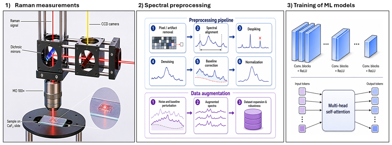
Figure 3.
(a) The 1D-CNN confusion matrix showing the distribution of true and predicted labels across the 36-class Raman dataset, with color intensity representing normalized prediction probability. The 1D-CNN achieved an overall accuracy of and a Matthews correlation coefficient (MCC) of . (b–c) Pseudo-3D sub-matrix representations mapping error structures within localized biological groups: (b) Staphylococcus species variants (MRSA, MSSA, MRSE, MSSE) and (c) Escherichia coli strain lines. Respective sub-macro accuracy and MCC metrics are detailed on the panel headers.
Figure 3.
(a) The 1D-CNN confusion matrix showing the distribution of true and predicted labels across the 36-class Raman dataset, with color intensity representing normalized prediction probability. The 1D-CNN achieved an overall accuracy of and a Matthews correlation coefficient (MCC) of . (b–c) Pseudo-3D sub-matrix representations mapping error structures within localized biological groups: (b) Staphylococcus species variants (MRSA, MSSA, MRSE, MSSE) and (c) Escherichia coli strain lines. Respective sub-macro accuracy and MCC metrics are detailed on the panel headers.
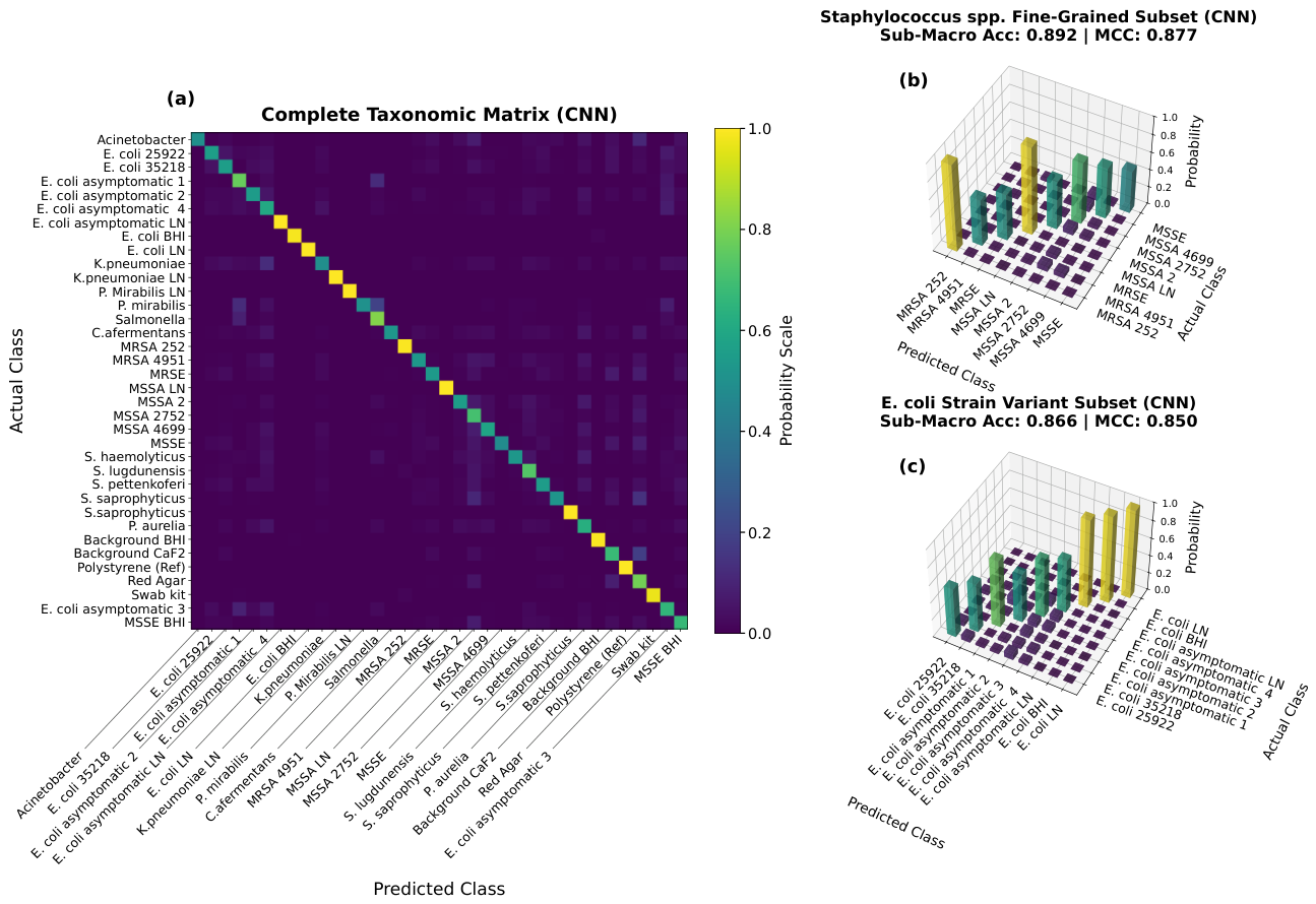
Figure 4.
(a) The ST confusion matrix showing the distribution of true and predicted labels across the 36-class Raman dataset. The ST achieved an overall accuracy of and a Matthews correlation coefficient (MCC) of . (b–c) Pseudo-3D sub-matrix representations mapping localized classification trends within specific groups: (b) Staphylococcus species variants (MRSA, MSSA, MRSE, MSSE) and (c) Escherichia coli strain lines, with respective sub-macro accuracy and MCC metrics detailed on the individual headers.
Figure 4.
(a) The ST confusion matrix showing the distribution of true and predicted labels across the 36-class Raman dataset. The ST achieved an overall accuracy of and a Matthews correlation coefficient (MCC) of . (b–c) Pseudo-3D sub-matrix representations mapping localized classification trends within specific groups: (b) Staphylococcus species variants (MRSA, MSSA, MRSE, MSSE) and (c) Escherichia coli strain lines, with respective sub-macro accuracy and MCC metrics detailed on the individual headers.
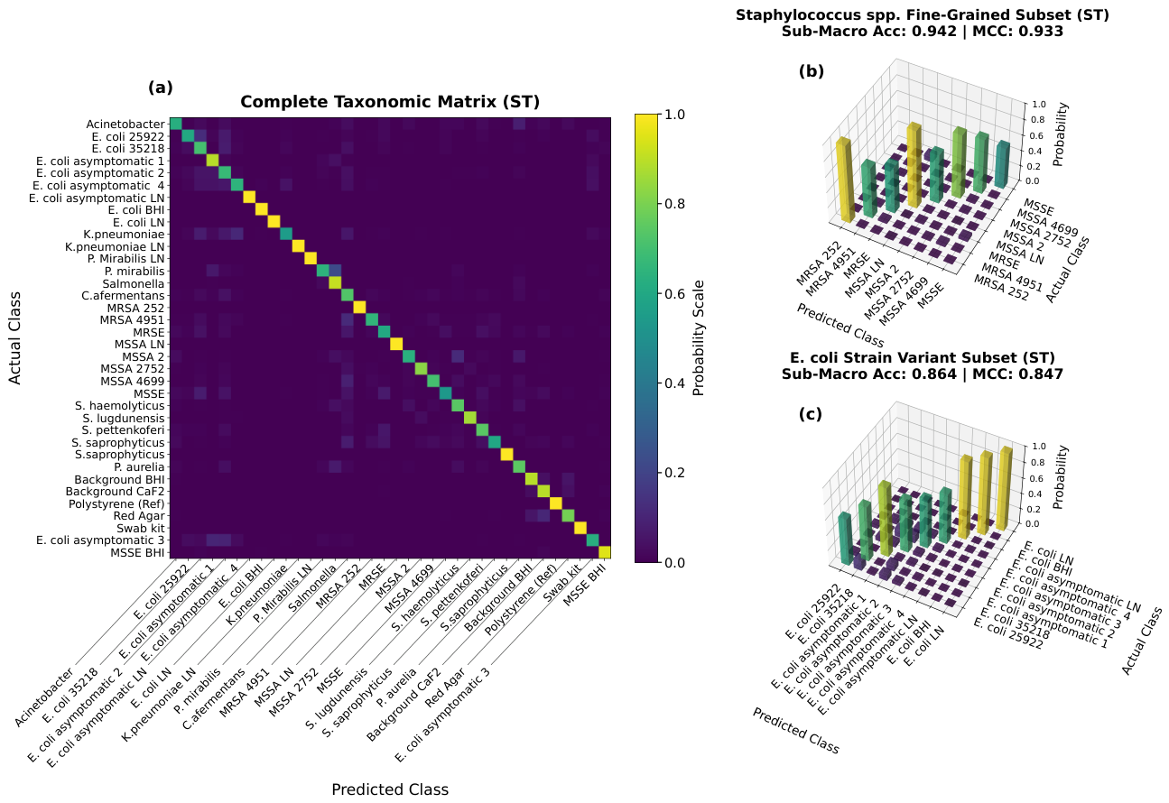
Figure 5.
Functional archetypes of 2D spectral attention matrices for Polystyrene. (a) A Biomarker Detector head (e.g., Head 13) exhibits strong positive correlation (, ) with the mean Raman spectrum, heavily anchoring on physical vibrational peaks. (b) An Inhibitory Attention head (e.g., Head 9) demonstrates negative spectral correlation (, ), mapping contrast regions to separate overlapping classes. (c) A Structural Context head (e.g., Head 11) shows near-zero correlation (, ), tracking baseline geometries and global token relationships. (d) The Model Consensus, representing the net integrated attention profile aggregated across all active heads. Top and left marginal plots overlay the class-averaged test spectrum (solid black line), with computationally fitted Gaussian peaks denoted by dashed lines to benchmark attention localizations.
Figure 5.
Functional archetypes of 2D spectral attention matrices for Polystyrene. (a) A Biomarker Detector head (e.g., Head 13) exhibits strong positive correlation (, ) with the mean Raman spectrum, heavily anchoring on physical vibrational peaks. (b) An Inhibitory Attention head (e.g., Head 9) demonstrates negative spectral correlation (, ), mapping contrast regions to separate overlapping classes. (c) A Structural Context head (e.g., Head 11) shows near-zero correlation (, ), tracking baseline geometries and global token relationships. (d) The Model Consensus, representing the net integrated attention profile aggregated across all active heads. Top and left marginal plots overlay the class-averaged test spectrum (solid black line), with computationally fitted Gaussian peaks denoted by dashed lines to benchmark attention localizations.
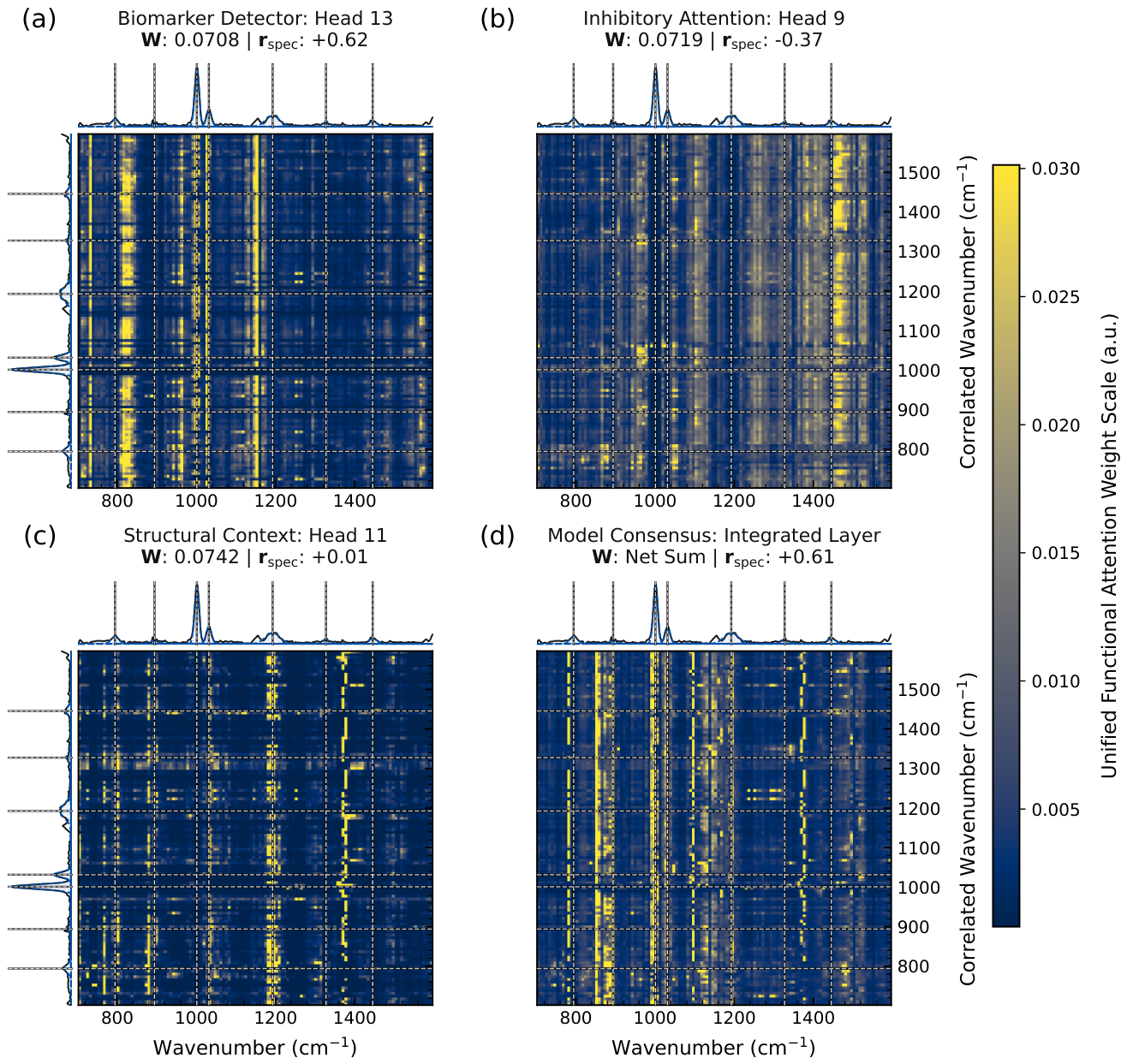
Figure 6.
Integrated Gradients (IG) feature attribution profiles for representative MSSA 4699 partitions. (a)–(b) True positive feature attribution profiles for the 1D-CNN and ST, overlaid on the class-averaged Raman spectrum (black traces). Positive and negative attributions relative to the dataset grand average are designated by red and blue bars, respectively. (c)–(d) Feature attribution maps computed for misclassified instances. The 1D-CNN exhibits significant spatial scattering and over-indexing in the 1400– region, whereas the ST maintains a relatively tighter attribution footprint.
Figure 6.
Integrated Gradients (IG) feature attribution profiles for representative MSSA 4699 partitions. (a)–(b) True positive feature attribution profiles for the 1D-CNN and ST, overlaid on the class-averaged Raman spectrum (black traces). Positive and negative attributions relative to the dataset grand average are designated by red and blue bars, respectively. (c)–(d) Feature attribution maps computed for misclassified instances. The 1D-CNN exhibits significant spatial scattering and over-indexing in the 1400– region, whereas the ST maintains a relatively tighter attribution footprint.
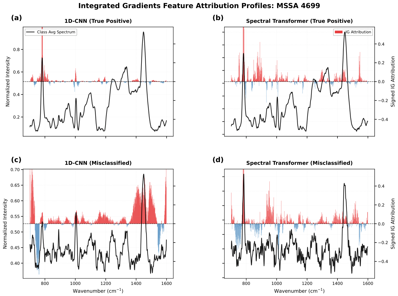
Figure 7.
Integrated Gradients (IG) feature attribution profiles for representativeE. coli35218 partitions. (a)–(b) Feature attribution profiles for true positive predictions across the 1D-CNN and ST models, overlaid on class-averaged Raman spectra (black traces). Red and blue bars indicate positive and negative attributions relative to the global baseline. (c)–(d) Feature attribution maps computed for misclassified instances. Similar to the MSSA profiles, the 1D-CNN demonstrates a vulnerability to localized disruptions in the 1400– lipid/amide window, while the ST misclassifications are driven by discrete, non-local perturbations.
Figure 7.
Integrated Gradients (IG) feature attribution profiles for representativeE. coli35218 partitions. (a)–(b) Feature attribution profiles for true positive predictions across the 1D-CNN and ST models, overlaid on class-averaged Raman spectra (black traces). Red and blue bars indicate positive and negative attributions relative to the global baseline. (c)–(d) Feature attribution maps computed for misclassified instances. Similar to the MSSA profiles, the 1D-CNN demonstrates a vulnerability to localized disruptions in the 1400– lipid/amide window, while the ST misclassifications are driven by discrete, non-local perturbations.
Disclaimer/Publisher’s Note: The statements, opinions and data contained in all publications are solely those of the individual author(s) and contributor(s) and not of MDPI and/or the editor(s). MDPI and/or the editor(s) disclaim responsibility for any injury to people or property resulting from any ideas, methods, instructions or products referred to in the content. |
© 2026 by the authors. Licensee MDPI, Basel, Switzerland. This article is an open access article distributed under the terms and conditions of the Creative Commons Attribution (CC BY) license (http://creativecommons.org/licenses/by/4.0/).
Copyright: This open access article is published under a Creative Commons CC BY 4.0 license, which permit the free download, distribution, and reuse, provided that the author and preprint are cited in any reuse.


