

Submitted:
05 June 2026
Posted:
08 June 2026
You are already at the latest version
Abstract
In-use heat transfer coefficient (HTC) measurements are useful for retrofit evaluation, heating system sizing, and thermal performance assessment in occupied homes. Quantifying the variance in the in-use HTC when, necessarily, utilising a range of assumptions and simplifications is therefore crucial, and also critical for further method development. Two empirical sensitivity analyses were used to explore how changes in commonly assumed in-use factors affect HTC estimates in occupied homes. The factors investigated were measurement uncertainty, solar gains, metabolic gains, boiler efficiency, water use, party wall heat transfer, and ventilation rate - parameters that are impractical or impossible to routinely measure, and as such default values are generally adopted. The sensitivity analyses used data from seven occupied homes and a single, common, HTC estimation method. Input distributions for each factor were derived from available data and current assumptions. A local sensitivity analysis examined how changes in each input affect the HTC and a global analysis quantified the contribution of the inputs’ variance to the HTC’s variance. Conducting parallel analyses enabled a more complete picture to be obtained, and the alignment of the two approaches provided confidence in their results. The factors with the greatest overall effects on the HTC were ventilation and party wall heat transfer; however, this was not the case for every home. In particular, HTCs from homes with higher occupancy exhibited stronger HTC sensitivity to metabolic gains and water use. The use of real data from occupied homes enables the results to be applicable to typical imperfect datasets. The results will inform future applications of in-use HTC measurements and methods for determining their uncertainty. Further work expanding this analysis to a larger dataset with more building typologies, and gathering data to define the sensitivity analysis more accurately would strengthen these conclusions.
Keywords:
in-use measurement
; heat transfer coefficient
; smart meter data
; SMETER
; building thermal performance
; domestic buildings
; Sensitivity analysis
1. Introduction
Climate change has led to the adoption of ambitious carbon emissions reduction targets in many countries; over 70 countries have committed to net zero targets, covering 76% of global emissions (United Nations Environment Programme 2023). Different decarbonisation pathways are planned by different governments, however, the importance of heating and cooling of buildings in this transition, accounting for 16% of global emissions (United Nations Environment Programme 2023), is widely acknowledged. Energy security concerns and high gas prices are also transforming energy policy, particularly in Europe where buildings are associated with 40% of energy consumption (including both construction and operation) (European Commission 2020). Governments are responding by raising ambition for improving the energy efficiency of buildings, such as the UK’s goal to reduce the final energy consumption from buildings by 15% by 2030 (DESNZ 2023). However, the widely reported performance gap between expected and actual performance of buildings (Johnston et al. 2015,Sunikka-Blank and Galvin 2012,Wingfield et al. 2009,Zero Carbon Hub 2014) challenges the delivery of such targets: neither their current performance nor the improvement upon retrofit are well characterised. Critically, unless this performance gap is effectively addressed, there is a significant risk that new homes, as addressed in the Future Homes Standard, would fail to achieve the intended energy and carbon reductions set out (MHCLG 2026). Compromised fabric performance may mean that the government targets to ensure homes are zero carbon ready without retrofitting, may be compromised. A range of technical and social factors contribute to the performance gap, that affect the design, build, and operation stages of the building (Wingfield et al. 2009). Critically, unless this performance gap is effectively addressed, there is a significant risk that new homes, as addressed in the Future Homes Standard, would fail to achieve the intended energy and carbon reductions (MHCLG 2026).
In response to the performance gap, the widespread adoption of the thermal characterisation of homes has been proposed to understand their real energy use, with a broad range of potential applications including providing insights and assurance to householders, assessment of construction and retrofit performance, and to support closing the performance gap (IEA EBC 2021). The thermal efficiency of a building is often measured through its steady state heat transfer coefficient (HTC), taken to be the average rate of heat transfer of the property and measured in Watts per Kelvin. The HTC is used directly or indirectly in many applications, such as in determining the reduction of energy consumption on retrofit or the appropriate size of a heating system, or indirectly in the calculation of energy performance certificate (EPC) ratings in the UK and many other countries. The HTC is defined as the ’heat flow rate divided by the temperature difference between two environments’ (BSI Standards 2017) comprising the sum of fabric and ventilation heat loss, although the ventilation loss is included implicitly rather than explicitly in most measurement methods (IEA EBC 2021).
The HTC may be measured for a real building using testing protocols on unoccupied homes (such as the aggregate heat loss (EN 2024)/coheating test or the Quick U-value of Buildings (QUB) test (Alzetto et al. 2018)) or through the evaluation of data from occupied buildings measured in situ, estimating the in-use HTC. The requirements for homes to be unoccupied, for 3-4 weeks in the most widely accepted method (the aggregate heat loss (EN 2024)/coheating test), limit the deployment of HTC testing methods. As a result, the in-use characterisation of occupied homes has received significant recent interest (e.g. IEA EBC Annexes 71 and 94 (IEA EBC 2021,IEA EBC 2024), UK Government Smart Meter Enabled Thermal Efficiency Ratings (SMETER) programme (Allinson et al. 2022,DESNZ 2019,DESNZ 2025)). Many of these in-use methods leverage the success of smart meter rollout programmes (GOV.UK 2023) to remotely capture energy use data; these may be combined with data from freestanding or other connected devices such as thermostats within homes to obtain the required data remotely (Allinson et al. 2022). However, measuring the heat transfer for in-use buildings is much more complex than unoccupied buildings or models; for example due to the reliance on the existing heating plant and distribution system, which is generally poorly characterised (Bennett et al. 2016), heat transfer between joined properties across party elements (Wingfield et al. 2009), which cannot be remotely measured, and variability in usage patterns of space and water heating (Eastwood 2025). Additional examples include metabolic gains (Porritt 2012), energy use outside the thermal envelope (for example, external lighting, workshops, hot tubs), solar gains (M. Li and Lomas 2020), and losses from water use and ventilation (Ritosa et al. 2023). Many of these factors are highly variable between and within homes (Eastwood et al. 2026), and are impossible to measure. The estimation of the in-use HTC thus requires assumptions to be made about the impact of these issues on heat transfer (IEA EBC 2021). The accuracy of the HTC derived from different in-use methods therefore varies as a combination of the model applied, in-situ measurements, and underlying assumptions about these additional factors. Standard values are available for some of the unmeasurable factors, such as those utilised in Energy Performance Certificate (EPC) assessments in the UK (BRE 2012), however recent work has uncovered inaccuracies in the energy consumption predictions produced by this method (the Standard Assessment Procedure, SAP) (Crawley et al. 2019,Few et al. 2023) potentially casting doubt on the accuracy of the standard values.
The impact of analytical assumptions and simplifications on a model’s outputs (where a method of in-use HTC measurement comprises data collection, processing and model application) can be investigated using sensitivity analysis. This has previously been used for a variety of purposes in the field of buildings and energy (Wei 2013), including design (Hopfe and Hensen 2011,Hygh et al. 2012) and the calibration of simulations (Sun and Reddy 2006,Westphal and Lamberts 2005), however not for occupied homes. Both local and global sensitivity analyses have been found to be valuable in assessing building energy simulation models (Hove et al. 2022,Wei 2013) and compliance tools (Halls et al. 2022), however these tools have not previously been applied to in-use models that utilise empirical data from occupied homes, and typically look at impact on energy consumption directly (Carlander 2021,Zhang et al. 2024) rather than building performance measurements such as the HTC.
This paper aims to provide insights into the potential impact of implicit and explicit assumptions and simplifications on in-use HTC measurements using commonly applied methods. The study applies sensitivity analyses to a simple and widely used in-use HTC measurement method, to explore the effect of typical assumptions on the measured in-use HTC and its variance. Whilst the specific impact of these different assumptions on the measured in-use HTC in any use case depends on the applied method, the study indicates key focus areas for data collection and method development. Two sensitivity methods are used: one examines how changing an assumption changes the estimated in-use HTC itself, and the other quantifies how much each assumption contributes to the variance in the estimated in-use HTC.
2. Dwelling Data
This study analyses a publicly available dataset of well-characterised homes (Allinson et al. 2022). The dataset includes that required for the analysis methods, as described below, and also contextual data (including occupancy) and a coheating test result for each home, serving as a baseline expectation of each home’s HTC; the dataset is available for download from Allinson et al. (2022). This paper presents analysis of data from seven of these homes in the north of England, collected in-situ as part of the Technical Evaluation of SMETER Technologies (TEST) project (Allinson et al. 2022). These homes were selected from the wider dataset of 30 homes (Allinson et al. 2022) due to the availability of sufficient data from both winter and summer, whilst avoiding data collected during strict COVID-19 lockdown restrictions as these may have disturbed typical routines. In this study the houses analysed are labelled A-G (corresponding to houses HH09, HH10, HH13, HH18, HH19, HH21, HH25 respectively).
The study homes were occupied after completion of a coheating test and are predominantly semi-detached (House A is detached) (Allinson et al. 2022,Allinson et al. 2022). They all have gas combination (combi) boilers and are predominantly naturally ventilated, as such these findings may not be applicable to, for instance, homes with heat pumps or MVHR systems. Some have kitchen or bathroom extractor fans but only one bathroom extractor fan is reportedly used (Allinson et al. 2022). Weather data were provided from a local station (a maximum of ~6km away). Occupants moved into the homes in late 2019 (Allinson et al. 2022), with data prior to occupation not considered in these analyses. In the global analysis presented in this paper three months of data beginning from the start of occupancy in winter, in addition to three months from summer 2020 (11th May - 11th August) were analysed. Three months was chosen as an appropriate duration of data to capture the range of occupant behaviour, technology performance (such as boiler efficiency) and conditions across each season: for instance, ground temperatures decrease and heating preferences change over winter, and window opening and time spent outside the home may be more variable in summer. In the local sensitivity analysis, the highest quality periods of winter data of sufficient length for analysis were selected from this larger dataset to obtain reliable in-use HTC measurements whilst the whole dataset was analysed for the global study. Days with energy, temperature, or solar radiation data missing were excluded from both analyses.
Electricity and gas consumption was monitored at 30-minute intervals, using an Emlite EMA1 smart meter (measurement uncertainty <1%) and a Honeywell BK-G4M connected to a pulse reader (measurement uncertainty <1%) respectively (Allinson et al. 2022). Internal temperatures in the kitchen, living room, bedrooms, bathroom and hall (5-7 sensors per house) were also recorded at 30-minute intervals, using Republic Of Things SmEILing sensors with measurement uncertainty of C (Allinson et al. 2022). Dwelling dimensions were taken from survey plan drawings (Allinson et al. 2022); in calculations undertaken for the analysis presented here it was assumed that internal walls were 0.15m thick and that ceilings were flat at a height of 2.5m. Area-weighted whole-house average temperatures were calculated for use in the analysis, treating the total area of the measured rooms as the total floor area of the house for this purpose. Daily electricity and gas consumption was calculated by converting to Watts using a calorific value of 39.2MJm−3 and a volume correction factor of 1.02264 for gas (UK Statutory Instruments 1996), and then taking the mean over 24 hours. Whilst all data were drawn from the same dataset, the specific data needs varied according to the sensitivity analysis method; this is discussed in the following.
3. Sensitivity Methods
Two methods were applied to investigate the sensitivity of in-use HTC analysis to various inputs: a local, one-at-a-time (OAAT) method and a global method (Sobol, (Sobol 2001)), which are outlined in more detail below. The OAAT analysis investigated the impact on the measured in-use HTC of changing the input assumptions to their most extreme values based on the range of potential values derived from available sources. Sobol analysis calculated the contribution to the variance of the in-use HTC measurement of variation in the input assumptions; the applied distributions of input assumptions were approximately bounded by the extremes used in the OAAT method (it was not possible to exactly match the changes in the inputs across the two analyses for all variables due to the differences in their approaches). Applying two different methods of sensitivity analysis enabled development of a more insightful picture of the sensitivity of the measured in-use HTC to analytical assumptions and simplifications: the OAAT approach allows changes in results to be clearly ascribed to an individual input, whereas the global Sobol method explores the relative importance of each input assumption to the variance of results and enables the joint effects of combinations of inputs to be assessed.
Both methods of sensitivity analysis explored the MLR (multilinear regression) method of HTC estimation. This is a very simple method, however is widely used both in coheating tests and with in-use data from occupied homes (IEA EBC 2021). The MLR method is derived from a simple heat balance, beginning by assuming that the net heat transfer of a home over 24 hours is zero: the heat input (e.g. from gas and electricity use and solar gains, among others) is equal to the heat lost through the building envelope over a day. The analysis thus uses daily averaged values of all inputs and regresses the heat input, P, against the difference between the internal and external temperatures () and the solar radiation (S), producing estimates of the HTC and solar aperture (g) as the respective gradients and is given in Equation (1), below
where , with e the boiler efficiency, G the gas consumption, and E the electricity consumption. An example of MLR analysis is shown in Figure 1 for House E.
For the sensitivity analyses the heat gains and losses in this model need to be disaggregated to explicitly include the factors to be investigated in the equation. The input assumption sensitivity variables used here are measurement errors, solar gains, the boiler efficiency, cold water losses, direct hot water losses, metabolic gains, party wall heat transfer, and ventilation heat transfer, with slight differences between the OAAT and Sobol methods due to the requirements of the different methods (detailed below). The disaggregated assumption model used is given below in Equation (2), a rearrangement and expansion of Equation (1).
where, in addition to the terms in Equation (1), n is the number of occupants, M is metabolic gains, and DHW is heat losses from hot water use (assuming this to be lost through the waste water system), CW is the cold water losses per occupant (due to incidental heating of cold water within the property), A and U the party wall area and U-value respectively, the temperature difference between the adjoining dwellings, the volumetric air change rate per hour, and V the internal volume of the building. The terms on the right hand side of the equation describe the following heat flows: is the heat gain from solar radiation; is the heat gain from gas use; E is the heat gain from electricity use; is the heat gain from occupants’ metabolic gains; is the heat loss from cold water use; is the heat loss from hot water use; is the heat transfer through the party wall - all per degree temperature difference between the internal and external environments, - and is the rate of ventilative heat loss. Further details of the two sensitivity analysis methods are given in the following.
3.1. One at a Time Sensitivity Analysis (OAAT)
The OAAT sensitivity analysis explored the effect on the HTC results obtained from the MLR model of changing each input assumption. Only winter data was used with this analysis, as the MLR HTC measurement method is generally only applicable to data from the heating season due to the signal-to-noise ratio needing to be of sufficient size. Input assumptions in Equation (2) were individually adjusted to their extreme value, with the remainder at their original values each time. The date ranges of data used for the OAAT analysis are given in Table 1.
3.2. Global Sensitivity Analysis: Sobol
Variance based sensitivity analyses such as the Sobol method decompose the variance in the output variable, here the in-use HTC, into fractions attributable to different inputs. The Sobol method repeatedly samples from the distributions specified for each input assumption, and uses these samples to evaluate the extended model in Equation (2) each time. This analysis was applied to the data from three months in winter and summer, with the average gas, electricity, internal-external temperature difference, and solar radiation values from each three month period in each season used in Equation (2). This averaging means the analysis does not reflect the extremes of either summer or winter in terms of conditions and occupant behaviours, but the overall season and the differences between them are represented.
The sampling used here was a quasi-Monte Carlo method: the Saltelli extension of the Sobol sequence, which has improved efficiency in comparison to a standard Monte Carlo approach (Saltelli 2002,Saltelli et al. 2010), implemented using the Python SALib library with the Saltelli sampler (Herman and Usher 2019). One thousand samples were produced for analysis of Equation (2) to enable sufficient representation of the input distributions. Three sensitivity indices were then calculated from the results of the Sobol analysis: S1, the first order index reflecting the individual contribution of each input to the output variance; S2, the contribution to the output variance of the interaction between two inputs; and finally ST, the total contribution to the output variance of each input, considering both its individual effect and any interactions with other inputs.
3.3. Sensitivity Inputs
In this section the sensitivity inputs for the two analyses are described, with details of how they were derived. These sensitivity inputs were selected based on the issues discussed in the introduction, and also what could reasonably be explicitly incorporated into the model for analysis. As mentioned above, the inputs were sometimes treated differently in the two sensitivity analyses due to their different implementations and aims, these are highlighted. Details of the homes used to determine the inputs are given in Table 2.
Internal-External Temperature Difference
The daily average internal-external temperature difference is a crucial term in the MLR model, and as such the impact of measurement errors in this parameter on the calculated in-use HTC were investigated. Typically the measurement error of this parameter would be taken from sensor specification sheets, which may not reflect the conditions of the sensor in a home, or could be unknown in the case of IoT devices. This factor was explored only in the OAAT analysis; given the structure of the model (Equation (2)) with T in almost every term the variation in this input would dominate the variance in the HTC in the Sobol analysis and thus obscure the contributions of other inputs. A 1oC error in the value was assumed, and so the MLR analysis in Equation (1) was repeated with and . The ±1oC error aims to account for measurement error in both the internal and external temperature sensors (0.2oC per sensor) as well as additional potential errors due to sensor placement e.g. with direct sunlight impacting or temperature stratification. It also aligns with the errors found in previous studies (Gauthier and Shipworth 2014,Jack et al. 2018,Stamp 2015).
Gas Power
The impact of measurement errors in the gas power on the calculated in-use HTC was investigated. This factor was only considered in the OAAT analysis, where both upper and lower bounds were explored. As for the temperature difference above, specified errors may not be applicable to the conditions of the meter in a home and signal issues could result in missing data, increasing the error in a daily average reading. Assuming a 1% error on the meter, in line with the measurement error of the gas meters used (Allinson et al. 2022), the analysis was repeated with the measured gas input multiplied by 1.01, and by 0.99. Other potential sources of error in gas data that have not been considered here are the calorific value and volume-to-pressure correction factor.
Electricity Power
As for the gas input, a 1% error on the meter is assumed (Allinson et al. 2022), and thus the analysis was repeated with the measured electricity multiplied by 1.01, and then by 0.99. This was again only considered in the OAAT sensitivity analysis.
Solar Radiation
The effect of solar gains was explored in both sensitivity analyses, as this is a dynamic quantity that is averaged to a daily value in the MLR model and not often measured on site for in-use methods. Impacts of solar gains were investigated considering measurement error for the OAAT method and through the variability of the effective solar aperture for the Sobol; in the OAAT analysis a measurement error of 5% was assumed (Allinson et al. 2022). The OAAT analysis also considered the potential impact of extreme shading, as the working assumption in the model is that the weather station data were applicable to the orientations and shading of the façades of the dwellings. Whilst impossible to represent all possible configurations, this was modelled by repeating the MLR analysis with daily average solar radiation calculated only using data from after midday.
Effective Solar Aperture
As stated above, in the Sobol analysis the impact of the variation of solar gains was explored through the variance of the effective solar aperture. This represents the impact of differing orientations and annually varying shading. This quantity was given a uniform distribution, with a lower bound of zero and an upper bound of an estimated maximum possible aperture (). The latter value was calculated according to the method used in the SAP energy model (BRE 2012), as the product of the glazed area, the total solar energy transmittance, and the frame factor, multiplied by 0.9 to reflect the ratio of typical transmittance to that at normal incidence. A value of 0.695 was used as the total solar energy transmittance as all homes have double glazing (Allinson et al. 2022) (the mean of the SAP double glazing values (BRE 2012)) and with no adjustments for aspects such as shading, to ensure the maximum possible aperture was calculated. These values are given in Table 2.
Boiler Efficiency
Boiler efficiency can vary seasonally (Orr and Summerfield 2009) and factors such as case losses are included in the given values (Allinson et al. 2022), but can in fact be heat gains to homes. To explore these sources of potential inaccuracy and uncertainty in the MLR model, the OAAT analysis repeated the MLR calculation with four different representations of the boiler efficiency: upper and lower fixed values, and upper and lower variable values. The fixed values and variable limits were selected based on in-situ monitoring of the efficiencies of condensing boilers (Orr and Summerfield 2009). This gave fixed upper and lower values of 90% and 80% respectively, with the upper variable heat output of W and the lower as W, where G is the gas consumption.
To investigate variability in the boiler efficiency in the Sobol analysis the boiler efficiency is assumed to be normally distributed around a value 2.1% less than the stated manufacturer’s efficiency (the stated efficiency is 89.3% for all houses (BRE 2019)), with a standard deviation of 2.3%. This is based on a histogram of the difference from stated efficiency at part load for 112 boilers (Hayton 2009), and results in a normal distribution with mean 0.872 (87.2%) and standard deviation 0.023 (2.3%).
Cold Water Losses
Cold water losses arise from heat transfer from a home into cold water within it, and its subsequent use by occupants and replacement with water at a lower temperature; the levels of this heat loss could potentially vary significantly from day to day and cannot be measured. In the OAAT analysis, these cold water losses are included as a simple modification to heat flow: they are directly subtracted from heat input. In the SAP energy model (BRE 2012) the assumption is that 40W is lost per person, which is thus assumed in the OAAT analysis.
The same 40W per person cold water loss was assumed to represent the mean value of this loss for the Sobol analysis. The losses were assumed to be normally distributed with a standard deviation of 13.3W (this value is then multiplied by the number of occupants as shown in Equation (2)). As no real distribution is available for this quantity the standard deviation of 13.3W was calculated to contain 99.7% of sampled values within the range of zero to twice the mean, aligning with the OAAT approach.
Hot Water Losses
Losses associated with domestic hot water (DHW) production, use and subsequent loss into waste water were estimated based on the BRE SAP analysis of monitoring data undertaken on UK homes by the Energy Saving Trust (EST) (Shorrock 2009) for both sensitivity analyses, as this cannot be easily quantified - typical available data is based on qualitative interviews (Allinson et al. 2022). The losses used here are calculated based on the number of occupants in addition to a standing daily amount (Shorrock 2009). It was assumed that each occupant contributes 1kWh of DHW loss per day, with an additional 1kWh lost per day, based on the percentage of useful gains and average DHW demand per occupant (Shorrock 2009).
In the OAAT analysis the MLR method was repeated with wide upper and lower bounds of hot water losses, subtracted directly from the heat input to the home to represent the potential for high uncertainty in the amount of hot water used in a home. The upper bound was taken to be double these losses (twice the hot water use) whilst the lower bound was zero losses (all heat was useful, no losses into the waste water). The same range was used to establish the distribution of hot water usage for the Sobol analysis. Hot water losses were assumed to be normally distributed with a standard deviation calculated to have 99.7% of values within the range of zero to twice the mean. They were multiplied by the number of occupants plus one (see Equation (2)), as for cold water losses. On this basis the mean is 41.7W (equivalent to 1kWh/day) with a standard deviation of 13.9W.
Metabolic Gains
Metabolic gains from occupants are impossible to measure, thus for both analyses metabolic gains were calculated using metabolic rate values (CIBSE 2015) for different categories of occupant. These rates were combined with the stated occupancy for each category within each home, as provided in the dataset, and adjusted for estimated percentages of the day in which they occupy the house (no differences between the weekend and weekdays were considered). These percentages were estimated based on typical working or school hours, and considered to be conservative, as they do not account for visitors to the home or homeworking. These assumptions are summarised in Table 3.
The OAAT analysis for metabolic gains incorporated an upper bound corresponding to double the heat gain, representing higher occupied hours and the potential for higher metabolic rates and visitors. In the Sobol analysis metabolic gains were assumed to be normally distributed, with the standard deviation once more calculated to have 99.7% of the values between zero and twice the mean. Using the values in Table 3, the gains per average occupant were calculated giving a mean of 67.23W per person per day, and a standard deviation of 22.4W.
Party wall heat transfer
For the OAAT analysis, party wall heat transfer was simplified as only a potential heat gain to the dwelling in question as the sensitivity is represented regardless. It was assumed that the party wall had a U-value of 2Wm−2K−1 (Lowe et al. 2007), and two different temperature differences between the dwellings of 1oC and 5oC. These temperature differences were selected to represent a modest and an extreme scenario respectively. It was also assumed that there was no party wall bypass operating, although no data were available about the dwellings to confirm this.
The three quantities that determine party wall heat transfer (party wall U-value and the two internal temperatures either side of it) will vary independently, however have not been considered as separate inputs in the Sobol analysis in order to achieve a single sensitivity index for party wall heat transfer. Both internal temperatures were assumed to be normally distributed with mean 20oC and standard deviation 0.67oC, with the latter calculated to have 99.7% of values within 19oC and 21oC. The mean temperature was chosen as a dwelling average based on the SAP energy model mean internal temperature calculation (BRE 2012), and the standard deviation calculated to align with the 1oC temperature difference in the OAAT analysis. The U-value was also modelled as a normal distribution with a mean of 2Wm−2K−1 and standard deviation 0.33Wm−2K−1 calculated to have 99.7% of the values within a ±1Wm−2K−1 range. These three distributions were combined to produce a range of values for party wall heat transfer equal to (as shown in Equation (2)). The party wall heat transfer values were used to estimate their inverse cumulative distribution function, enabling the use of inverse transform sampling to allow the inclusion of this custom distribution in the sensitivity analysis (Devroye 2010).
Ventilation heat transfer
The ventilation heat loss from a dwelling is implicitly included in the in-use HTC calculated by the MLR model (it includes all heat losses during the period of measurement). However, it has been explicitly calculated for the sensitivity analyses to explore the impact of fixed assumed ventilation rates on the measured fabric-only in-use HTC. In the OAAT analysis two levels of increase in ventilation heat loss above the nominal value in the SAP energy model (BRE 2012) were considered to explore the impact on the calculated fabric in-use HTC of these magnitudes of change: an additional 0.25h−1 and an additional 0.5h−1, corresponding to 50% and 100% increases on the 0.5h−1 typically assumed (BRE 2012,CIBSE 2015). These were modelled by subtracting the ventilation heat loss calculated in Equation (3) from the measured HTC,
For the Sobol analysis variation in ventilation heat transfer was also modelled by variation in the number of air changes per hour (), as shown in Equation (2). The distribution of the air change rate was assumed to be normal, with mean 0.46h−1 and standard deviation 0.15h−1. These values were taken from the average of the results of four different studies of ventilation and air quality exploring naturally ventilated homes using winter PFT (PerFluorocarbon tracer gas) measurements (Crump et al. 2005,EST and AECOM 2019,Kukadia and White 2006,McKay et al. 2010).
4. Results
In the following section the results of the two sensitivity analyses using the physically informed limits outlined above are presented. The individual household percentage differences from the original MLR HTC (OAAT) and total sensitivity indices (Sobol) were used to rank the sensitivity inputs per house by the size of their effect. An overall ranking across all households was then produced for each of the sensitivity inputs using the order of the average rank numbers of each input for all houses. Total sensitivity indices were used for the Sobol rankings, however second order sensitivity indices were not significant (indicating only minor joint effects), and as such the total indices are very similar to the first order indices.
Internal-External Temperature Difference
The effect of changing the temperature difference inputs was explored only in the OAAT analysis, with the lower bound () producing a greater percentage difference to the standard MLR HTC than the upper bound for all houses. The lower and upper bounds of the temperature difference were ranked 4th and 6th respectively of all 16 investigated inputs, producing average absolute changes in the calculated in-use HTC of 9.1% and -7.8%. The greatest percentage changes were for House B for both the upper (-10%) and lower bounds (12.1%), whilst the smallest were for House G (-6.3% and 7.1% for the upper and lower bounds respectively).
Gas Power
The gas power was also explored only in the OAAT analysis, and produced symmetrical results for the upper and lower bounds. As such, it was ranked as one variable with a ranking across all houses of 13th. The percentage change was small, with an average of . The greatest change of 1% was for House D, whilst the smallest percentage difference of 0.8% was found for Houses B, E, and F.
Electricity Power
Electricity power was again only considered in the OAAT analysis, and as for the gas power had a symmetrical effect. The percentage change in the measured in-use HTC measurement was smaller than gas for all houses, with an average absolute change of 0.13%, ranking 16th. The maximum change produced was 0.2% for Houses B, E, and F, with the lowest for House D. This is the opposite of the gas power, and is reflected in the raw data with a much higher gas-to-electricity ratio in House D than B, E, and F.
Solar Gains
The sensitivity to solar gains was explored in both the OAAT and Sobol analyses, however different sources of uncertainty were considered. The OAAT analysis incorporated a 5% increase to the solar radiation measurement and an extreme shading scenario where only solar gains after midday were considered, whilst the Sobol analysis modelled shading by assuming the solar aperture was uniformly distributed between 0 and a calculated maximum aperture.
Due to the formulation of the MLR model (Equation (1)), the 5% increase in solar radiation produced no change to the HTC measured for all houses in the OAAT. Instead, this caused the estimate of the solar aperture to decrease, with the change accounted for in this value rather than the in-use HTC. The extreme shading scenario in the OAAT analysis ranked 12th out of 16, with an average change of -0.75%. This result reflects that this change produced a decrease in in-use HTC for most houses, but surprisingly for House B a measured in-use HTC increase of 1.5% in House B, with the average change of the other houses excluding B equal to -1.5%. The greatest change produced was -2.5%, for House G, with the smallest of -0.4% in the results for House F.
The variation of the solar aperture in the Sobol analysis ranked 6th out of 7 in winter, and 1st of 7 in the summer with average total sensitivity indices of 0.10 and 0.48 for the respective seasons. In both winter and summer the solar aperture variation had the highest contribution for House A, and the lowest contribution for House F.
Boiler Efficiency
In the OAAT analysis the effect of the boiler efficiency on the measured in-use HTC was explored using upper and lower bounds of both fixed and variable efficiencies to explore errors in the efficiency due to age or case gains, and variation in efficiency due to seasonal factors. The lower variable and fixed bounds in the OAAT analysis produced the greatest percentage differences from the original HTC measurement, with the fixed efficiencies overall also producing larger changes than the variable model; these results are found in Table 4.
It is not unexpected that the lower bounds have a greater effect than the upper bounds, as they are further from the values used in the standard MLR analysis (89.3% (Allinson et al. 2022)) than the upper bounds. The fixed bounds are also expected to have greater effect than the variable bounds as the latter are closer to the original value used across the range of efficiencies.
For the Sobol analysis the boiler efficiency was assumed to be normally distributed and the variability had the 4th and 7th greatest impacts out of 7 for winter and summer respectively, with corresponding mean total sensitivity indices of 0.12 in winter and just 0.007 in summer when space heating is not in use. In winter House D had the highest sensitivity index of 0.21, with the lowest for House B at 0.05. In summer House D again had the highest sensitivity index of 0.03, with the lowest of 0.0002 for House A. House D having the highest sensitivity index in both seasons reflects the findings for the electricity and gas measurement errors above of this house having a higher gas-to-electricity ratio than others.
Metabolic Gains and Water Use
Metabolic gains and losses from cold and hot water use are all assumed to be proportional to the number of occupants in a house, and as such the results for these inputs are presented together. These factors were considered in both types of sensitivity analysis using the same basis for their bounds or distributions, producing the results shown in Table 5.
The three occupancy factors have the same order in the ranking for both analyses and seasons, with the effect of the number of occupants clearly demonstrated by the results for House F which has the highest occupancy of 6, and correspondingly the highest percentage differences and total sensitivity indices for all three inputs.
Party Wall Heat Transfer
The effects of party wall heat transfer were considered in the OAAT analysis by exploring 1oC and 5oC temperature differences with a fixed U-value and in the Sobol analysis by assuming the house and adjoining dwelling internal temperatures and the U-value were normally distributed and combining these distributions. In the OAAT analysis the larger temperature difference produced the greatest percentage difference as would be expected, with the 5oC temperature difference input ranked 2nd out of 16, and the 1oC temperature difference ranked 11th. In the Sobol analysis the party wall input was overall ranked 2nd out of 7 in both seasons.
The OAAT analysis with a 5oC temperature difference produced a mean HTC percentage difference from the standard MLR result of 11.2%, with a maximum of 16.3% for House B and a minimum of 7.7% for House D. The 1oC analysis produced a correspondingly smaller mean difference of 2.2%, with a maximum of 3.3%, again for House B, and a minimum of 1.5% for House D. House B has one of the larger party wall areas (Table 2) and a low internal temperature corresponding to the low gas consumption mentioned above, whilst House D has much lower party wall area and a higher internal temperature. The results for the Sobol analysis have total sensitivity indices of 0.11 and 0.13 for winter and summer respectively. In both seasons House B again had the highest index (winter 0.15 and summer 0.16), and House F had the lowest (winter 0.07 and summer 0.08), with the occupancy related gains dominating in the latter.
Ventilation Heat Transfer
Both analyses explored the effects of varying ventilation heat transfer, in the OAAT analysis with two levels of air changes per hour (), and with normally distributed air change rates for Sobol. Ventilation had a large effect in both analyses, with the higher air change rate for OAAT ranking 1st and the lower 7th, whilst for Sobol in winter it was ranked 1st and in summer 5th. The higher additional air change rate (0.5h−1) OAAT analysis had a mean percentage difference of -13.2%, with the greatest change in House E of -17.5% and the lowest -11.3% for House D. The impact of the smaller increase in ventilation rate are half these, and thus the same houses are found to have the highest and lowest changes for this analysis. In the Sobol analysis of winter data the average sensitivity index was 0.41, with House E producing the maximum index of 0.48 and House F the lowest of 0.27. In summer there was an average index of 0.11, with the lowest House A at 0.01 and the highest 0.2 for House D.
4.1. Results Summary
The sensitivity results for each house are shown in Figure 2, with the percentage change in HTC for the OAAT analysis and the total sensitivity index for the Sobol analysis presented. Where multiple versions of an input were changed in the OAAT analysis the version shown is specified. These results highlight the differences between the change in measured in-use HTC and the change in the variance of the measured in-use HTC; the impact of variables in both the winter and summer are also shown in the variance in the measured HTC.
5. Discussion
The results outlined above demonstrate the relative importance of different model assumptions and simplifications when calculating the in-use HTC of case study homes using the MLR method (Equation (1)). In the results of the Sobol analysis the total sensitivity index has been evaluated, accounting for both the individual contribution of variation in an input to the HTC variance and the joint contribution of any interactions with other inputs. The individual effect indices, excluding joint contributions, are not reported because the difference between the separate individual and joint indices is small in all cases. Given the known covariance of several effects such as between different occupancy-related factors and that between solar gains and factors affected by external temperature this is a perhaps surprising result; however, this is caused by the independent sampling of input distributions in the presented analysis. This independent sampling was undertaken because no known and generalisable relationship exists to establish co-variant relationships for each home within the MLR model.
Ventilation heat loss was ranked highly in both sensitivity analyses using winter data, and was not insignificant in the summer Sobol analysis. This suggests that, under the potential variability in ventilation rate applied in this analysis, ventilation can make a sizeable contribution to both the variance of the in-use HTC and uncertainty in its value. The greater effect in winter likely reflects the increased internal-external temperature difference, and therefore heat flow, in this season; in winter ventilation heat loss is likely to be primarily driven by infiltration (Roberts and Lomas 2025), whilst in summer increased purpose-provided ventilation is likely (Roberts et al. 2021). Heat transfer via party walls similarly ranks highly for both analyses, with the same rankings for Sobol in winter and summer although with slightly larger total sensitivity indices in the latter season. Other studies have found party wall heat transfer to be among the largest sources of variability in the HTC, resulting in overestimations of dwelling heat loss (Eastwood 2025). Party wall heat transfer is dependent upon the temperature difference between the adjoining properties, which is often assumed to be zero in analysis for convenience or practical reasons. It may be mitigated in measurements by placing temperature sensors in the adjoining house, for a solid party wall, but this is often not possible. Alternatively, heat flow at spot-locations can be measured and the results scaled across the whole element then incorporated into the in-use HTC analysis model, this requires the use of heat flux sensors, a more intrusive measurement method. The results presented here suggest that both the ventilation rate and party wall heat loss can be important when measuring the in-use HTC, and that they therefore represent potential sources of uncertainty in that in-use HTC which can change over time as conditions and neighbouring property temperatures change. Evaluation of their contribution to heat flow can improve the accuracy of HTC measurements, if not addressed, their incorporation into uncertainty estimates can support appropriate interpretation of the results.
The effects of gas and electricity metering errors on in-use HTC measurements were explored only in the OAAT analysis, producing consistently small changes relative to other inputs. This is because the expected errors are relatively small and supports the use of smart meter data on a wide scale for thermal performance assessment (DESNZ 2019). The homes with the greatest change in measured in-use HTC for gas metering errors also have the smallest change for electricity, and vice versa, corresponding to the relative levels of use of each in those homes.
In the analysis of summer data, outside the heating season, the boiler efficiency was ranked last in the Sobol analysis, contributing very little to the HTC variance. In the OAAT and Sobol analyses of winter data, however, the boiler efficiency is an important factor in estimating the in-use HTC. Boiler efficiency is often incorporated into thermal performance assessment methods as a constant based on the tabulated values, such as the PCDB (BRE 2019); however, this does not accurately represent several effects. Case losses are assumed to be losses (to external environments) in efficiency measurement; however, if the boiler is within the heated envelope these contribute to heating the home. Additionally, efficiencies are obtained in laboratory testing, which deviates from performance in real homes (Bennett et al. 2019). Boiler efficiency also varies with external temperature due to changes to the inlet and return temperatures, changes to the flow temperature (where it is variable), intermittency of heating (Bennett et al. 2019) and, in colder temperatures, the boiler may be unable to meet the heat demand of the dwelling. The impact of boiler efficiency on measured in-use HTC may be mitigated through heat metering, which is costly and disruptive, on-board boiler data (which may be difficult to access and of unknown accuracy), or through a testing protocol developed to evaluate or minimise the uncertainty. A contrasting approach, which also applies to heat pump installations, is to evaluate a characteristic of the home that explicitly incorporates the efficiency of the heating system, such as the HPLC (Heat Power Loss Coefficient (Chambers and Oreszczyn 2019,Hollick et al. 2020)), the joint performance of the building fabric and heating system.
Solar gains have far greater effect in the summer Sobol analysis than either of the winter sensitivity analyses, which is expected from the relatively larger heat gains from solar radiation compared to the remainder of heat inputs into dwellings in summer compared to winter.
The importance of seasonal impacts via temperature changes affecting boiler efficiency and solar gains is demonstrated by the ranking of the inputs from the results of the seasonal Sobol analyses, shown in Table 6. These results highlight the importance of the season in which the data are collected. While it is currently rare to use data from outside the heating season for thermal performance assessment, it would be beneficial to extend the testing season and these seasonal factors may have implications for the methods used to do so (e.g. (Hollick et al. 2020)).
The individual rankings for each house, shown in Table 6 vary significantly, with the most obvious cause being the number of occupants. In House F, with six occupants, the three inputs that are conventionally assumed to be proportional to the occupancy of a house (metabolic gains, DHW and CW losses) rank higher than for other, lower occupancy homes. This is clearly demonstrated by the bar charts in Figure 3, where (a) and (c) are for a house with one occupant (C), and (b) and (d) are for House F. This is to be expected from the formulation of the inputs in this study, but highlights the importance of occupancy to in-use HTC measurement. These effects have increasing impact as heating energy input drops, such as with improving home thermal efficiency. High efficiency homes, such as new homes or retrofitted homes, are therefore likely to exhibit lower signal-to-noise ratios than lower efficiency homes (Li 2022), such as the (typical for the UK) homes studied here. Improving methods to accommodate such issues, or to better enumerate unmetered gains and losses, will improve accuracy and are important to enable in-use characterisation of all homes, including those with high thermal efficiency.
6. Conclusions
This paper reports the results from two sensitivity analyses of in-use HTC measurement in real occupied homes, studying the impact of parameters that affect empirically evaluated in-use HTCs, but are either impossible to or at least not typically measured. An in-use HTC model, MLR, was used for both sensitivity analyses; MLR methods are commonly used in thermal performance estimation (Allinson et al. 2022,IEA EBC 2021) and are closely related to other quasi-static methods, such as the Siviour method; the results presented here are expected to indicate the relative importance and approximate size of the effects of the assumptions in all such methods.
Results from local OAAT and global Sobol analyses are presented to indicate both the impact of input parameters on in-use HTC measurements and their variances, and the relative importance of different factors. The input factors considered were measurement errors, solar gains, metabolic gains, boiler efficiency, domestic hot water use, cold water use, party wall heat transfer and increases in ventilation rate; these were explicitly incorporated into the MLR equation to enable analysis using simple theoretical representations. Input data for these factors are not widely available or extensive; they were drawn from a range of sources. Better characterisation of the distributions of the input assumptions for the homes would enhance future analysis and the conclusions that can be drawn.
The sensitivity of in-use HTC measurements to the input factors was found to vary across the homes under study and between the summer and winter seasons. Ventilation heat loss, boiler efficiency, and party wall heat transfer were shown to have the consistently greatest impacts on the results, and are among the most difficult to measure on an individual home basis. Other factors such as the occupancy related inputs (metabolic gains and water use) and heat from solar gains have highly variable effects dependent on the number of occupants and the season the data were collected in, and as such will be inconsequential for some results, but very important for others. Measurement errors within the reported errors of the sensors were not found to have a large impact, providing confidence in the use of such measured data.
This study highlights the challenges of estimating in-use HTCs in homes that are subjected to different weather, occupant practices and technology performance. The need to account for these factors depends on the application of the in-use HTC: its use in policy and practice (Allinson et al. 2022,IEA EBC 2021). In applications where the occupants remain in the same home, such as to evaluate the impact of retrofit or to empirically size a heating system, occupant-related factors may not pose a significant practical impediment to the use of an in-use HTC since such heat gains may be assumed to remain approximately constant.
Where the in-use HTC is used to indicate the thermal efficiency of a home for use by other (potential) occupants, such as in an Energy Performance Certificate (BRE 2012), however, occupant-related factors introduce higher uncertainty in the result. Similarly, although not all directly explored in this study, heating system use (set-point and duration), change of temperatures in adjoining properties and in-home technologies may all affect in-use HTC measurements through their impact on the internal temperature distribution, which is not necessarily well-characterised by a daily average. However, the uncertainty in energy performance of homes exposed by performance gap literature (Johnston et al. 2015,Sunikka-Blank and Galvin 2012,Wingfield et al. 2009,Zero Carbon Hub 2014) and results from trials (Allinson et al. 2022) suggests that measurement of the in-use HTC could reduce uncertainty for many homes compared to incumbent survey and modelling methods. Further research is required to explore the accuracy requirements of different applications of in-use HTCs, to develop appropriate frameworks to integrate these insights into policy and practice.
Developments in the methods for in-use HTC measurement can improve the accuracy and transferability of results, and support clearer comparison with other methods of HTC measurement such as coheating tests (Gori and Elwell 2018). However, the burden of additional measurement may be costly and intrusive, unless integrated into other technologies such as heating systems and controllers and home energy management systems. In the absence of this additional monitoring, understanding the effects of assumptions on in-use HTC measurements, is crucial in evaluating their uncertainty. Reliable in-use HTCs are expected to be central to policy based on thermal performance measurement (BEIS 2020,Rathmell et al. 2020), future development of in-use HTC estimation methods will be possible as data become more widely available.
Since the analysis in this study utilised in-use data from a relatively small sample of real homes, the results should be interpreted as indicative of the impact of factors that cause variability in in-use HTC measurements rather than being directly applicable to all homes. Expanding this analysis to a larger and more varied sample of homes will enable deeper insights, which requires similarly detailed data collection from such homes. Further, it is expected that the inputs will have different effects for different analysis methods and for homes of different thermal efficiency. In particular, estimation of accurate in-use HTCs is expected to be challenging when metered heat input is low, such as for high efficiency homes, homes subjected to deep retrofit and underheated homes. Further research is required to address these issues, and it is noted that different in-use HTC estimation methods may not be affected equally by such factors, and thus there may not be a single ’most appropriate method’ across the stock or even for a single home across different seasons and operation.
The results presented in this study are highly dependent on the definitions and values of the inputs to the sensitivity methods; the distributions for the Sobol analysis or the change made for the OAAT analysis. Two key inputs that would benefit from further data are water heating and the party wall heat transfer. Work to inform these, and other inputs, to make them more representative of the real ranges of values experienced at different times of year would allow for greater insight into the uncertainty of the measured in-use HTCs.
This work has enabled better understanding of the impacts of un-measured and un-measureable quantities on in-use HTC measurements, highlighting ventilation heat loss and party wall heat transfer as dominant sources of uncertainty. This provides crucial information for both the assessment and use of in-use HTC measurements, and further development of the measurement and uncertainty calculation methods.
Author Contributions
FH: Conceptualisation, Software, Formal Analysis, Writing - Original Draft, Visualisation; JW: Conceptualisation, Formal Analysis; BR: Writing - Review & Editing; KR: Writing - Review & Editing; CG: Writing - Review & Editing; CE: Conceptualisation, Writing - Review & Editing, Supervision, Funding Acquisition
Funding
The authors disclosed receipt of the following financial support for the research, authorship, and/or publication of this article: This work was supported by the EPSRC Centre for Research into Energy Demand Solutions (grant number EP/R035288/1).
Institutional Review Board Statement
This study uses pseudonymised, secondary data that is published and as such no ethical approval was required.
Informed Consent Statement
Not applicable.
Data Availability Statement
The dataset used in this study is available for download from https://reshare.ukdataservice.ac.uk/856978/.
Acknowledgments
The authors wish to acknowledge the invaluable contribution of all of the team members that delivered the UK government Technical Evaluation of SMETER Technologies (TEST) project, and especially those that were instrumental in the collection of the data that were analysed for this paper.
Conflicts of Interest
The authors declared no potential conflicts of interest with respect to the research, authorship, and/or publication of this article.
References
- Allinson, D., J. Crawley, C. Elwell, D. Farmer, F. Fylan, D. Glew, C. Gorse, A. Hardy, F. Hollick, D. Johnston, K.J. Lomas, D.L. Loveday, D. Miles-Shenton, J. Parker, L. Reevell, B.M. Roberts, G. Roberts, F. Thomas, and J. Wingfield. 2022. Technical Evaluation of SMETER Technologies Project, Phase 2 Data: Heat Transfer Coefficients, In-Use Temperature and Energy Data, Local Weather, Dwelling Information, and Occupancy Surveys From 30 English Dwellings, 2019-2021. [CrossRef]
- Allinson, David, Ben Roberts, Kevin Lomas, Dennis Loveday, Chris Gorse, Adam Hardy, Thomas Thomas, Dominic Miles-Shenton, David Johnston, David Glew, Kambiz Rakhshanbabanari, Fiona Fylan, David Farmer, Cliff Elwell, Jenny Crawley, Frances Hollick, Jez Wingfield, Gavin Roberts, and Lee Reevell. 2022. Technical Evaluation of SMETER Technologies (TEST) project: full report. pp. 183.
- Alzetto, Florent, Guillaume Pandraud, Richard Fitton, Ingo Heusler, and Herbert Sinnesbichler. 2018. QUB: A fast dynamic method for in-situ measurement of the whole building heat loss. Energy and Buildings 174, 124–133. [CrossRef]
- BEIS. 2020. THE DOMESTIC PRIVATE RENTED PROPERTY MINIMUM STANDARD. Technical report.
- Bennett, George, Clifford Elwell, Robert Lowe, and Tadj Oreszczyn. 2016. The Importance of Heating System Transient Response in Domestic Energy Labelling. Buildings 6, 29. [CrossRef]
- Bennett, George, Cliff Elwell, and Tadj Oreszczyn. 2019. Space heating operation of combination boilers in the UK: The case for addressing real-world boiler performance. Building Services Engineering Research and Technology 40, 75–92. [CrossRef]
- BRE. 2012. SAP2012 - The Government’s Standard Assessment Procedure for Energy Rating of Dwellings. Technical report, BRE.
- BRE. 2019. BRE Product Characteristics Database.
- BSI Standards. 2017. BS EN ISO 52016-1:2017 Energy performance of buildings - Energy needs for heating and cooling, internal temperatures and sensible and latent heat loads. Technical report.
- Carlander, Jakob. 2021. On the Effect of Occupant Behavior and Internal Heat Gains on the Building’s Energy Demand A case study of an office building and a retirement home. Ph. D. thesis, University of Gävle.
- Chambers, Jonathan D. and Tadj Oreszczyn. 2019. Deconstruct: A scalable method of as-built heat power loss coefficient inference for UK dwellings using smart meter data. Energy and Buildings 183, 443–453. [CrossRef]
- CIBSE. 2015. Guide A Environmental design. Technical report.
- Crawley, Jenny, Phillip Biddulph, Paul J Northrop, Jez Wingfield, and Tadj Oreszczyn. 2019. Quantifying the Measurement Error on England and Wales EPC Ratings. Energies 12.
- Crump, Derrick, Sani Dimitroulopoulou, Richard Squire, David Ross, Bridget Pierce, Martin White, Veronica Brown, and Sara Coward. 2005. Ventilation and indoor air quality in new homes. Pollution Atmospherique, 71–76.
- DESNZ. 2019. Smart Meter Enabled Thermal Efficiency Ratings (SMETER) Innovation Programme.
- DESNZ. 2023. Energy Company Obligation: Great British Insulation Scheme (2023-2026) & Amendments to ECO4 regulations. Technical report.
- DESNZ. 2025. Green Homes Grant (GHG) SMETER project evaluation.
- Devroye, Luc. 2010. Complexity questions in non-uniform random variate generation. [CrossRef]
- Eastwood, M. 2025. Variability in the Heat Transfer Coefficient of dwellings. Ph. D. thesis, Loughborough University.
- Eastwood, Max, David Allinson, Matthew Li, and Ben M Roberts. 2026. Measuring the in-use thermal performance of dwellings: improving the precision by accounting for variability. Journal of Building Physics 49(4), 530–555. [CrossRef]
- EN. 2024. EN 17887-1:2024 - Thermal performance of buildings - In situ testing of completed buildings - Part. Technical report.
- EST and AECOM. 2019. Ventilation and indoor air quality in new homes. Technical report.
- European Commission. 2020. Energy efficiency in buildings. Technical report.
- Few, Jessica, Despina Manouseli, Eoghan Mckenna, Martin Pullinger, Ellen Zapata-webborn, Simon Elam, David Shipworth, and Tadj Oreszczyn. 2023. The over-prediction of energy use by EPCs in Great Britain : A comparison of EPC-modelled and metered primary energy use intensity. Energy & Buildings 288, 113024. [CrossRef]
- Gauthier, Stephanie and David Shipworth. 2014. Variability of thermal stratification in naturally ventilated residential buildings. In Building Simulation and Optimization Conference, pp. 1–7.
- Gori, Virginia and Clifford A. Elwell. 2018. Estimation of thermophysical properties from in-situ measurements in all seasons: quantifying and reducing errors using dynamic grey-box methods. Energy and Buildings 167, 290–300. errors method. [CrossRef]
- GOV.UK. 2023. Energy security bill factsheet: Smart metering.
- Halls, Benjamin, Steven K. Firth, and Kevin J. Lomas. 2022. The influence of dwelling energy efficiency on the sensitivity of inputs to a steady-state energy model. In Building Simulation Conference Proceedings, pp. 1727–1734. International Building Performance Simulation Association. [CrossRef]
- Hayton, J. 2009. A meta-analysis of boiler test efficiencies to compare independent and manufacturers’ results. Technical report, BRE.
- Herman, J and W Usher. 2019. Salib.
- Hollick, Frances P, Virginia Gori, and Clifford A Elwell. 2020. Thermal performance of occupied homes : A dynamic grey-box method accounting for solar gains. Energy & Buildings 208, 109669. [CrossRef]
- Hopfe, Christina J. and Jan L.M. Hensen. 2011. Uncertainty analysis in building performance simulation for design support. Energy and Buildings 43, 2798–2805. [CrossRef]
- Hove, M. Y.C. Van, M. Delghust, and J. Laverge. 2022. Global sensitivity analysis for large scale building energy models: importance of building stock size and convergence. In Building Simulation Conference Proceedings, pp. 2307–2314. International Building Performance Simulation Association. [CrossRef]
- Hygh, Janelle S., Joseph F. DeCarolis, David B. Hill, and S. Ranji Ranjithan. 2012. Multivariate regression as an energy assessment tool in early building design. Building and Environment 57, 165–175. [CrossRef]
- IEA EBC. 2021. Annex 71 - Building Energy Performance Assessment Based on In-situ Measurements.
- IEA EBC. 2024. Annex 94 - Validation and Verification of In-situ Building Energy Performance Measurement Techniques.
- Jack, Richard, Dennis Loveday, David Allinson, and Kevin Lomas. 2018. First evidence for the reliability of building co-heating tests. Building Research and Information 46, 383–401. [CrossRef]
- Johnston, D, D Miles-Shenton, and D Farmer. 2015. Quantifying the domestic building fabric ’performance gap’. Building Services Engineering Research and Technology 36, 614–627. [CrossRef]
- Kukadia, V and M White. 2006. Monitoring ventilation in homes built before 1995: A pilot study. Technical report.
- Li, Matthew. 2022, 5. Thermal performance of UK dwellings: assessment of methods for quantifying whole-dwelling heat loss in occupied homes. [CrossRef]
- Lowe, R J, J Wingfield, Mimmm Ceng, M Bell, J M Bell, and Msci Phys. 2007. Evidence for heat losses via party wall cavities in masonry construction. Building Services Engineering Research and Technology 28, 1–19.
- M. Li, D. Allinson and K. Lomas. 2020. Estimation of building heat transfer coefficients from in-use data: impacts of unmonitored energy flows. International Journal of Building Pathology and Adaptation.
- McKay, S, D Ross, I Mawditt, and S Kirk. 2010. Ventilation and indoor air quality in Part F 2006 homes. Technical report.
- MHCLG. 2026. The future homes and building standards: Building circular 01/2026. Technical report, MHCLG.
- Orr, Georgina and Iain Summerfield. 2009. Final report : In-situ monitoring of efficiencies of condensing boilers and use of secondary heating position. Technical report.
- Porritt, Stephen Michael. 2012. Adapting UK Dwellings for Heat Waves. PhD Thesis, Institute of Energy and Sustainable Development, De Montfort University, Leicester.
- Rathmell, Alex, Tadj Oreszczyn, Juliet Phillips, Sam Thomas, and Chris Jofeh. 2020. Towards a protocol for metered energy savings in UK buildings. Technical report, Green Finance Institute: Coalition for the Energy Efficiency of Buildings.
- Ritosa, Katia, Dirk Saelens, and Staf Roels. 2023. A large scale artificial dataset to evaluate the impact of on-board monitoring set-ups on the heat transfer coefficient assessment. Energy & Buildings 289, 113061. [CrossRef]
- Roberts, Ben M., David Allinson, and Kevin J. Lomas. 2021, 10. Evaluating methods for estimating whole house air infiltration rates in summer: implications for overheating and indoor air quality. International Journal of Building Pathology and Adaptation 41(1), 45–72. [CrossRef]
- Roberts, B.M., Rossi V. Gorse C. Li M. and K.J. Lomas. 2025. Airtightness retrofit and construction practices, unintended consequences, and ventilation practices: Gathering evidence to improve airtightness in the uk housing stock. Technical report, UK Government.
- Saltelli, Andrea. 2002. Making best use of model evaluations to compute sensitivity indices. Computer Physics Communications 145, 280–297. [CrossRef]
- Saltelli, Andrea, Paola Annoni, Ivano Azzini, Francesca Campolongo, Marco Ratto, and Stefano Tarantola. 2010. Variance based sensitivity analysis of model output. design and estimator for the total sensitivity index. Computer Physics Communications 181, 259–270. [CrossRef]
- Shorrock, L.D. 2009. Analysis of the EST’s domestic hot water trials and their implications for amendments to BREDEM and SAP. Technical report, BRE.
- Sobol, I. M. 2001. Global sensitivity indices for nonlinear mathematical models and their monte carlo estimates. Mathematics and Computers in Simulation 55, 271–280. [CrossRef]
- Stamp, Samuel Francis. 2015. Assessing uncertainty in co-heating tests : Calibrating a whole building steady state heat loss measurement method. Ph. D. thesis.
- Sun, Jian and T. Agami Reddy. 2006. Calibration of building energy simulation programs using the analytic optimization approach (rp-1051). HVAC and R Research 12, 177–196. [CrossRef]
- Sunikka-Blank, Minna and Ray Galvin. 2012. Introducing the prebound effect: the gap between performance and actual energy consumption. Building Research & Information 40, 260–273. [CrossRef]
- UK Statutory Instruments. 1996. The gas (calculation of thermal energy) regulations.
- United Nations Environment Programme. 2023. Emissions Gap Report 2023: Broken Record - Temperatures hit new highs, yet world fails to cut emissions (again). [CrossRef]
- Wei, Tian. 2013. A review of sensitivity analysis methods in building energy analysis. Renewable and Sustainable Energy Reviews 20, 411–419. [CrossRef]
- Westphal, Fernando Simon and Roberto Lamberts. 2005. Building simulation calibration using sensitivity analysis. In Ninth International IBPSA Conference, pp. 1331–1338.
- Wingfield, Jez, Malcolm Bell, Dominic Miles-Shenton, Tim South, and Bob Lowe. 2009. Lessons from stamford brook. understanding the gap between designed and real performance. pp. 1–137.
- Zero Carbon Hub. 2014. Closing the gap between Design and as-built performance. Evidence Review Report.
- Zhang, Hu, Wei Tian, Jingyuan Tan, Juchao Yin, and Xing Fu. 2024, 6. Sensitivity analysis of multiple time-scale building energy using bayesian adaptive spline surfaces. Applied Energy 363. [CrossRef]
Figure 1.
MLR analysis of House E, plotted here when solar radiation, S, is equal to zero. The gradient of the line, the HTC, is (157±31)WK−1.
Figure 1.
MLR analysis of House E, plotted here when solar radiation, S, is equal to zero. The gradient of the line, the HTC, is (157±31)WK−1.
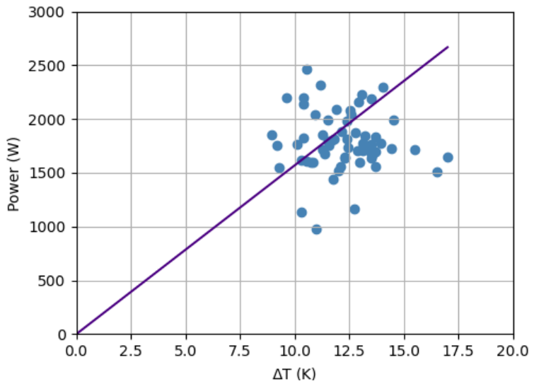
Figure 2.
The results per house of both sensitivity analyses for the inputs studied both in terms of their impact on the calculated in-use HTC (OAAT) and their contribution to its variance (Sobol). For the OAAT analysis, the results shown are for the lower bound, variable boiler efficiency model; for the 5oC temperature difference across the party wall; and for the additional 0.5h−1 ventilation.
Figure 2.
The results per house of both sensitivity analyses for the inputs studied both in terms of their impact on the calculated in-use HTC (OAAT) and their contribution to its variance (Sobol). For the OAAT analysis, the results shown are for the lower bound, variable boiler efficiency model; for the 5oC temperature difference across the party wall; and for the additional 0.5h−1 ventilation.
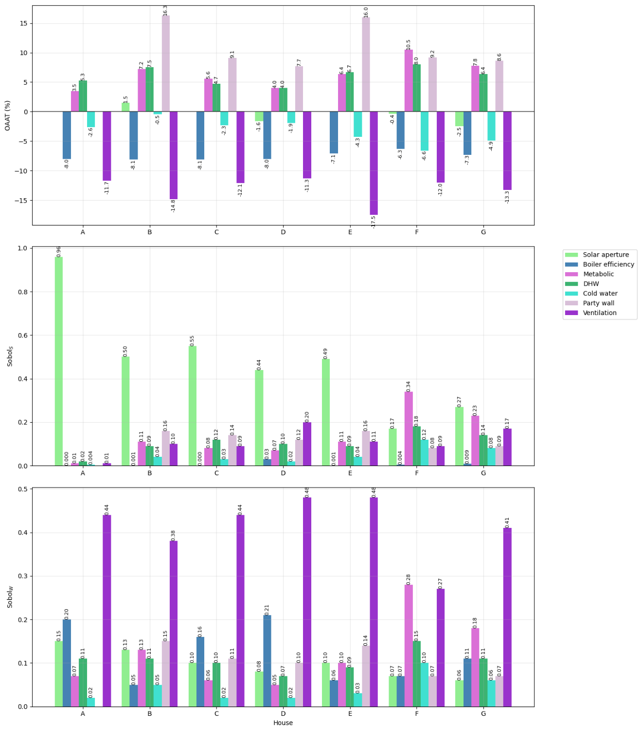
Figure 3.
The contributions to the variance of the measured in-use HTC of each input from the winter and summer Sobol analyses for House C, with one occupant, and House F with six.
Figure 3.
The contributions to the variance of the measured in-use HTC of each input from the winter and summer Sobol analyses for House C, with one occupant, and House F with six.
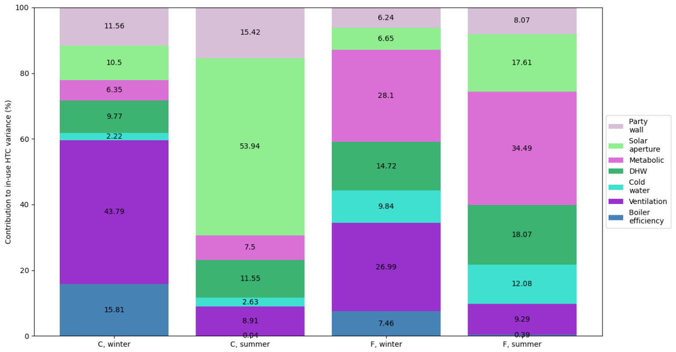

Table 1.
Dates bounding the analysis periods used in the OAAT sensitivity analysis.
| House | Start date | End date | Number of days |
|---|---|---|---|
| A | 27/11/19 | 21/12/19 | 23 |
| B | 20/12/19 | 09/03/20 | 81 |
| C | 09/12/19 | 09/03/20 | 92 |
| D | 16/12/19 | 09/03/20 | 85 |
| E | 22/12/19 | 21/02/20 | 62 |
| F | 23/12/19 | 09/03/20 | 78 |
| G | 09/02/20 | 09/03/20 | 30 |
Table 2.
Details of the homes used in the sensitivity analyses (Allinson et al. 2022).
Table 2.
Details of the homes used in the sensitivity analyses (Allinson et al. 2022).
| House | Num. | Volume | Party wall | Winter | Summer |
| occupants | (m3) | area (m2) | (m2) | (m2) | |
| A | 1 | 107.6 | 0 | 1.9 | 6.6 |
| B | 2 | 165.3 | 27.1 | 2.5 | 2.9 |
| C | 1 | 107.4 | 15.9 | 1.5 | 1.8 |
| D | 1 | 107.4 | 15.8 | 1.5 | 1.7 |
| E | 2 | 167.1 | 30.1 | 2.2 | 2.9 |
| F | 6 | 211.4 | 33.6 | 3.0 | 2.9 |
| G | 4 | 175.3 | 27.7 | 2.2 | 3.0 |
Table 3.
Assumed metabolic gains (CIBSE 2015) and occupancy percentages for various types of occupant.
Table 3.
Assumed metabolic gains (CIBSE 2015) and occupancy percentages for various types of occupant.
| Occupant | Daily metabolic | Occupant | Percentage of day |
| gains (W) | in house (%) | ||
| Adult male | 115 | Working adult | 55 |
| Adult female | 98 | Unemployed adult | 70 |
| Child | 86 | Retired adult | 85 |
| Child | 60 |
Table 4.
Results from the OAAT analysis for the four different boiler efficiency models.
| Rank | Mean | Max. | House | Min. | House | |
| /16 | % diff | % diff. | with max. | % diff. | with min. | |
| Low, fixed | 3 | -8.9 | -10 | D | -8 | F |
| High, fixed | 14 | 0.7 | 1.2 | A | 0.6 | B, E, F |
| Low, variable | 5 | -7.6 | -8.1 | B, C | -6.3 | F |
| High, variable | 15 | 0.6 | 1.1 | A | 0.2 | B |
Table 5.
Results for the occupancy related factors for both sensitivity analyses: metabolic gains; cold water losses (CW) and hot water losses (DHW). The effect is the in-use HTC difference for OAAT, and the contribution to the variance in the in-use HTC for Sobol.
Table 5.
Results for the occupancy related factors for both sensitivity analyses: metabolic gains; cold water losses (CW) and hot water losses (DHW). The effect is the in-use HTC difference for OAAT, and the contribution to the variance in the in-use HTC for Sobol.
| Method | Season | Metabolic | DHW | CW | |
|---|---|---|---|---|---|
| Rank | OAAT | 8 | 9 | 10 | |
| (OAAT/16; | Sobol | Winter | 4 | 5 | 7 |
| Sobol/7) | Summer | 2 | 5 | 6 | |
| Mean effect | OAAT | 6.4% | ±6.1% | -3.3% | |
| Sobol | Winter | 0.12 | 0.11 | 0.04 | |
| Summer | 0.14 | 0.11 | 0.05 | ||
| Maximum | OAAT | 10.5% | ±8% | -6.6% | |
| effect | Sobol | Winter | 0.28 | 0.15 | 0.1 |
| Summer | 0.34 | 0.18 | 0.12 | ||
| House | OAAT | F | F | F | |
| with max. | Sobol | Winter | F | F | F |
| Summer | F | F | F | ||
| Minimum | OAAT | 3.5% | ±4% | -0.5% | |
| effect | Sobol | Winter | 0.05 | 0.07 | 0.02 |
| Summer | 0.01 | 0.02 | 0.004 | ||
| House | OAAT | A | D | B | |
| with min. | Sobol | Winter | D | D | D |
| Summer | A | A | A |
Table 6.
The rankings of the total sensitivity indices from the Sobol analysis for each of the 8 houses in both winter (W) and summer (S).
Table 6.
The rankings of the total sensitivity indices from the Sobol analysis for each of the 8 houses in both winter (W) and summer (S).
| Input | A | B | C | D | E | F | G | |||||||
| W | S | W | S | W | S | W | S | W | S | W | S | W | S | |
| Boiler eff. | 2 | 6 | 6 | 7 | 2 | 7 | 2 | 6 | 6 | 7 | 5 | 7 | 3 | 7 |
| Ventilation | 1 | 4 | 1 | 4 | 1 | 4 | 1 | 3 | 1 | 3 | 2 | 5 | 1 | 3 |
| CW | 6 | 5 | 7 | 6 | 7 | 6 | 7 | 7 | 7 | 6 | 4 | 4 | 6 | 6 |
| DHW | 4 | 2 | 5 | 5 | 5 | 3 | 5 | 4 | 5 | 5 | 3 | 2 | 4 | 4 |
| Metabolic | 5 | 3 | 3 | 3 | 6 | 5 | 6 | 5 | 3 | 4 | 1 | 1 | 2 | 2 |
| Solar | 3 | 1 | 4 | 1 | 4 | 1 | 4 | 1 | 4 | 1 | 7 | 3 | 7 | 1 |
| Party wall | 2 | 2 | 3 | 2 | 3 | 2 | 2 | 2 | 6 | 6 | 5 | 5 | ||
Disclaimer/Publisher’s Note: The statements, opinions and data contained in all publications are solely those of the individual author(s) and contributor(s) and not of MDPI and/or the editor(s). MDPI and/or the editor(s) disclaim responsibility for any injury to people or property resulting from any ideas, methods, instructions or products referred to in the content. |
© 2026 by the authors. Licensee MDPI, Basel, Switzerland. This article is an open access article distributed under the terms and conditions of the Creative Commons Attribution (CC BY) license (http://creativecommons.org/licenses/by/4.0/).
Copyright: This open access article is published under a Creative Commons CC BY 4.0 license, which permit the free download, distribution, and reuse, provided that the author and preprint are cited in any reuse.