Submitted:
05 June 2026
Posted:
08 June 2026
You are already at the latest version
Abstract
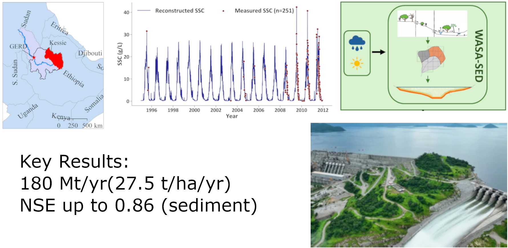
The Upper Blue Nile Basin contributes about 60% of the Nile River’s annual streamflow but faces severe sediment-related challenges driven by intense monsoonal erosion and reservoir siltation. Accurate estimation of suspended sediment concentration (SSC) and sediment load in large, data‑scarce watersheds remains difficult due to sparse monitoring and complex supply‑limited transport dynamics. This study develops a hybrid approach that combines machine‑learning‑based reconstruction of SSC with process‑based hydrological and sediment modelling for the Kessie watershed, a major sediment source upstream of the GERD.
The approach combines Random Forest (RF) based SSC reconstruction from only 251 sparse samples with a two-stage calibration of the WASA-SED model. Using hydrologically informed predictors, the RF algorithm substantially outperformed traditional sediment rating curves and other machine‑learning algorithms, increasing the coefficient of determination from 0.23 to 0.693. The reconstructed daily SSC yielded a mean annual sediment load of 180.7 Mt/yr. The model performed well, particularly at monthly scales for 1995–2011, and reproduced dominant hydrological and sediment regimes. Trend analysis indicated no significant changes in rainfall, streamflow, or sediment load.
The combining approach captures monsoon‑driven sediment fluxes and provides reliable sediment load estimates that support improved reservoir sedimentation assessment, erosion-risk evaluation, and transboundary water‑resources planning in data‑scarce tropical highlands.
Keywords:
data-scarce
; erosion
; process-based modelling
; machine learning
; reservoir sedimentation
; sediment load estimation
; Upper Blue Nile Basin
1. Introduction
The Upper Blue Nile Basin (UBNB) contributes about 60% of the Nile River’s annual streamflow and an even larger share of its sediment load (70–80%), with basin-wide sediment delivery estimated at 100–140 million tons per year (Mt/yr) [1,2,3]. These substantial water and sediment fluxes make the basin central to regional water security, hydropower development, irrigation expansion, and transboundary cooperation among Ethiopia, Sudan, and Egypt. The high sediment load is driven by intense seasonal rainfall, steep topography, and widespread rain-fed agriculture on highly erodible soils, creating some of Africa’s most severe erosion problems and posing major challenges for reservoir siltation, downstream water quality, and long-term agricultural productivity [4,5].
Within this broader context, the Kessie watershed represents a strategically important and hydrologically representative sub-basin located entirely within Ethiopia and upstream of the Grand Ethiopian Renaissance Dam (GERD). Recent studies project that the GERD will trap 92–97% of incoming sediment, leading to an estimated annual storage loss of ~0.28% (189 Mm³/yr) and significantly affecting downstream reservoirs such as Roseires [6]. Accurate upstream sediment load estimates from the Kessie watershed are therefore critical.
It spans the Amhara (91%) and Oromia (9%) regional states, supports an estimated 17.1 million population as of 2020, based on the global gridded population dataset of Liu et al. (2024), and exhibits pronounced topographic relief, with elevations ranging from 993 m at the outlet to over 4,200 m in the highlands. Land-use change between 2000 and 2020 has been substantial, with built-up areas expanding by 277% while dense vegetation and wetlands have declined markedly, based on the global land cover and land use change dataset of [8]. These transformations, combined with the seasonal rainfall regime, generate highly nonlinear, hysteretic, and event-driven sediment transport dynamics that conventional methods fail to capture.
Conventional power-law sediment rating curves (SRCs) remain the most common approach for estimating continuous sediment loads from intermittent SSC samples and continuous streamflow records. However, SRCs assume a stationary streamflow-sediment relationship and fail to represent antecedent moisture effects, clockwise or anti-clockwise hysteresis loops, and the shift between supply-limited and transport-limited conditions that characterize the Ethiopian highlands [4,9]. As a result, peak SSC values often occur at moderate flows early in the rainy season when freshly exposed soils are abundant, whereas lower SSC values may occur at higher flows later in the season due to sediment depletion and dilution. Consequently, conventional rating curves frequently underestimate sediment peaks and overestimate baseflow transport.
Recent advances in the development of hydrologically informed predictors combined with ensemble machine learning have shown strong potential to overcome these limitations by explicitly encoding dominant physical drivers, such as lagged and cumulative precipitation, flow history, hysteresis indices, and seasonal cycles, without relying on rigid parametric assumptions. Applications of machine learning in the Blue Nile basin have demonstrated substantial improvements over conventional methods [1,10]. At the same time, semi-distributed process-based models such as WASA-SED can represent spatial heterogeneity in runoff generation, erosion, and sediment routing when supplied with reliable continuous inputs [11,12]. Hybrid approach that integrates machine-learning reconstruction of sparse SSC observations with process-based watershed simulation are therefore particularly valuable in data-scarce African highlands. In basins where SSC data consist of only a few hundred intermittent samples, continuous reconstruction is essential because process-based models require daily sediment input for robust calibration and long-term sediment yield estimation [1,10,13]. Despite these needs, such hybrid approaches have rarely been applied at the sub-basin scale with explicit assessment of predictor-importance analysis and regime-specific evaluation.
This study addresses these gaps in the Kessie watershed. It develops and benchmarks tree-based machine learning models for daily SSC reconstruction using a systematic development of primary and ancillary predictors with permutation importance analysis, benchmarking of Random Forest (RF), Gradient Boosting (GB); Quantile Random Forest (QRF), and SRC models. It then implements and calibrates the WASA-SED model using the reconstructed sediment loads within a two-stage (hydrology-then-sediment) optimization framework. The integrated model is evaluated across daily-to-monthly timescales and flow/sediment regimes using duration curve analysis. Finally, annual hydro-climatic trends in rainfall, streamflow, and sediment load are evaluated using non-parametric tests to determine whether significant changes exist and to establish a baseline for predictor analysis. By integrating sparse event-based observations with continuous hydro-meteorological records and a physically based semi-distributed model, the resulting framework provides a replicable methodology for improved water-resources planning, reservoir sedimentation assessment, and erosion-risk management in similar data-scarce monsoonal catchments of the UBNB and beyond.
2. Materials and Methods
2.1. Study Area Description
The Kessie watershed lies in north-central Ethiopia within the UBNB, spanning Amhara (91%) and Oromia (9%) regional states. It covers 65,784 km² with a main river channel 609 km long descending from headwaters at approximately 2,545 m to the outlet at 993 m (mean watershed elevation ~2,300 m). The maximum elevation in the watershed exceeds 4,200 m. Pronounced topographic relief drives runoff generation, erosion intensity, and fluvial transport. The climate is monsoonal with a mean annual rainfall of 1,207 mm and reference evapotranspiration of 895 mm estimated using Enku’s temperature method [14], yielding a positive water balance that sustains perennial flow despite strong seasonality. Land cover is dominated by cropland (>31,000 km²), with secondary classes of dense short vegetation, tree cover, open water, semi-arid vegetation, and expanding built-up areas (Table 1). Population growth and land-use intensification exert increasing pressure on water and sediment resources, consistent with broader UBNB trends documented in multiple SWAT-based studies [3,15].
Figure 1.
Location of the Kessie watershed within (a) Northeast and Eastern Africa with the Upper Blue Nile Basin (UBNB), and (b) a detailed map showing the watershed boundary, rainfall stations, and the outlet.
Figure 1.
Location of the Kessie watershed within (a) Northeast and Eastern Africa with the Upper Blue Nile Basin (UBNB), and (b) a detailed map showing the watershed boundary, rainfall stations, and the outlet.

2.2. Data Collection
Available daily hydro-meteorological data were obtained for the study area, including streamflow (Q), rainfall (P), temperature (T), and relative humidity (H) for the period 1995-2011. Streamflow records were obtained from the Kessie gauging station operated by Ethiopia’s Ministry of Water and Energy (MoWE). Rainfall, temperature, and relative humidity data were collected from a network of 49 meteorological stations distributed across the watershed and provided by the Ethiopian Meteorological Institute (EMI). All hydro-meteorological variables were available as continuous daily time series. These variables (Q, P, T, and H) served as direct inputs to the WASA-SED model.
SSC observations were also obtained from MoWE. In contrast to the continuous hydro-meteorological records, SSC measurements were available only as 251 intermittent samples collected during previous field campaigns. These samples ranged from 0.14 to 42.33 g/L with a median value of 0.72 g/L. Approximately 70% of the measurements were recorded during the wet season, reflecting the strong monsoon-driven sediment transport dynamics typical of the UBNB. Such sparse and event-based sediment observations are common in data-limited catchments in the region, as reported in previous studies [1,10].
The pronounced seasonality of rainfall and the event-driven nature of sediment transport necessitate the reconstruction of continuous daily SSC time series to enable process-based hydrological and sediment modeling. A summary of some datasets used in this study is presented in Table 2.
2.3. Machine Learning–Based SSC Modeling
2.3.1. Hydrologically Informed Predictors
To better represent the dominant hydrological and seasonal processes controlling sediment mobilization in monsoonal highland catchments, a comprehensive set of 18 predictors was derived from the continuous daily Q and daily P records. The continuous P for the watershed was calculated using inverse distance weighting (IDW) interpolation from the network of 49 meteorological stations. The hydrologically informed predictors were selected to represent key features including antecedent wetness conditions, flow history, hysteresis behavior, and seasonal periodicity that strongly influence SSC in the UBNB [9,16].
The predictor set include instantaneous Q, P, daily change in Q (dQ = Qₜ – Qₜ₋₁), a hysteresis index, the 7-day moving average of Q (Q_MA7), and lagged values of both Q and P at intervals of 1, 3, 7, 14, and 21 days. Seasonal cycles were encoded using sine and cosine transformations of the Julian day (Sin_J and Cos_J). Antecedent moisture conditions were represented by the 7-day antecedent Precipitation Index (API_7), calculated recursively with a decay constant k = 0.85 using the formula APIₜ = Pₜ + k × APIₜ₋₁ (where Pt is the watershed-average daily precipitation (mm) on day t, APIt-1 is the API value from the previous day). The value of k = 0.85 was chosen following common practice in Ethiopian highland studies, as it effectively balances the influence of recent rainfall events while retaining memory of antecedent wetness over approximately one week [4,9].
The hysteresis index (HIt) was computed as the deviation of instantaneous flow from its short-term moving average, defined as HIt = Qt - Q_MA7, t, which distinguishes rising-limb from falling-limb conditions and captures event-scale supply-limited dynamics. This developed set of predictors was designed to help machine learning models go beyond simple Q–SSC relationships and explicitly account for non-stationary, supply-limited behavior and hysteresis effects frequently observed in the region.
Permutation feature importance was assessed by measuring the mean decrease in R² upon random permutation of each feature. Due to multi-collinearity among lagged P and lagged Q features, the importance values should be interpreted as the collective contribution of related feature groups rather than the unique contribution of each feature. A complete description of all 18 predictors, including units and hydrological interpretation, is provided in Supplementary Table S1.
2.3.2. Benchmark Model: SRC
The classical power-law SRC served as the baseline model:
Where; parameters a and b were estimated via ordinary least-squares regression on log₁₀(SSC) versus log₁₀ (Q + 1), with predictions back-transformed and clipped to non-negative values. This mirrors common practice in data-scarce Ethiopian studies [4,10] but is known to underperform due to hysteresis and non-stationarity.
2.3.3. Machine Learning Models
Three ensemble tree-based regressors were implemented using the Python package scikit-learn [17]. GB (sequential shallow trees minimizing residuals), RF (bootstrap aggregation and random feature selection for robustness), and QRF (median quantile for skewed distributions and inherent uncertainty quantification). These were chosen for their ability to handle non-linearity, noise, and feature interactions for UBNB sediment applications when data are limited [13,18,19].
The uncertainty in the RF-predictions of daily SSC was quantified using the ensemble distribution of the individual trees. For each day, predictions were obtained from all 500 trees in the forest. The 95% prediction interval was then defined by the 2.5th and 97.5th percentiles of these 500 tree-level predictions. This interval represents the model’s internal variability and provides a measure of predictive uncertainty without assuming a specific error distribution.
2.3.4. Model Training, Hyper-Parameter Tuning, and Validation
To respect temporal autocorrelation and avoid information leakage, the SSC dataset was split chronologically into a 70% training period and a 30% independent validation period. Hyper-parameter tuning was performed using RandomizedSearchCV (30 iterations) with 5-fold time-series cross-validation within the training set, using the coefficient of determination (R²) as the primary scoring metric. This chronological splitting and cross-validation strategy preserves the temporal structure of the data and ensures no future information leaks into the training process.
2.3.5. Model Evaluation Metrics
Performance was quantified using a comprehensive suite: R² (fraction of variance explained), RMSE (root mean squared error; sensitive to large prediction errors; g/L), MAE (mean absolute error, average magnitude of prediction errors; g/L), MAPE (mean absolute percentage error, relative prediction error; %), and a custom composite score emphasizing goodness-of-fit while rewarding low absolute/relative errors:
Visual assessment included observed vs. predicted scatter plots (1:1 line) and time-series overlays to evaluate episodic peak reproduction.
2.4. Hydrological and Sediment Modelling
2.4.1. Model Description
The Water Availability and Sediment Analysis – Semi-Distributed (WASA-SED) model is a process-based, deterministic, and time-continuous modelling framework developed to simulate coupled hydrological and sediment dynamics in complex river basins [20,21]. Its physically grounded process representations and hierarchical spatial discretization make it particularly suitable for meso-scale catchments ranging from approximately 100-10,000 km² [22]. The model has been widely applied in semi-arid, tropical highland, and mountainous environments [23], with recent studies demonstrating its versatility across diverse landscapes in Brazil [24], Ethiopia [11], and Mediterranean Spain [12].
2.4.2. Spatial Discretization and Model Setup
The watershed was delineated using 30 m SRTM DEM and hydrography data (river network and drainage lines). Land-use (Landsat/GlobCover) and soil (Harmonized World Soil Database) information were integrated into the model setup. Spatial discretization was performed using the lumpR tool [25], which defined Landscape Units (LUs) as unique combinations of land use, soil type, and slope class, organized into representative topo-sequences, resolved into terrain-component instances for efficient and spatially lumped simulation with WASA-SED. This discretization approach balances data requirements and computational feasibility while capturing key spatial heterogeneity, consistent with recent applications in the region [11].
2.4.3. Simulation Period and Warm-Up Phase
Daily simulations were conducted for the period 1995–2011. A two-year warm-up (1995–1996) was used to stabilize initial water and sediment stores and ensure equilibrium before calibration [26]. Variable-state files generated at the end of the warm-up period (e.g., groundwater, soil moisture, interflow, river, reservoir, and sediment storage) were used as initial conditions for the calibration run. Similarly, state files produced at the end of calibration were used to initialize the validation period, ensuring continuity of internal water and sediment stores across simulation phases.
2.4.4. Calibration and Validation Strategy
Model calibration followed a robust two-stage sequential approach. First, hydrological parameters were optimized against observed streamflow then sediment-related parameters were calibrated using RF-reconstructed sediment loads, while keeping the hydrological parameters fixed. This step-wise strategy ensures that sediment processes build on a stable and physically consistent hydrological foundation.
Parameter optimization in both stages employed the Dynamically Dimensioned Search (DDS) algorithm [27], implemented in the parallelized R package ppso [28]. Thirty-two parallel DDS runs, with up to 3,200 function evaluations each, were conducted to minimize the root mean square error (RMSE) as the objective function at the watershed outlet. In the first stage, hydrological parameters were calibrated against observed streamflow. In the second stage, sediment parameters were calibrated against the RF-reconstructed sediment loads while keeping the hydrological parameters fixed. The final calibrated parameters are presented in Table 3.
Calibration was performed for 1997–2006, and validation was performed for 2007–2011, allowing assessment of model transfer-ability under varying hydro-climatic conditions.
2.4.5. Performance Evaluation and Duration Curves
Model performance was evaluated using a suite of complementary metrics: the Nash–Sutcliffe Efficiency (NSE) to assess the model’s ability to capture temporal dynamics, the Percent Bias (PBIAS) to quantify systematic over- or underestimation, and the Kling–Gupta Efficiency (KGE) to provide an integrated measure of correlation, bias, and variability [29,30]. These metrics were computed at both daily and monthly timescales, with greater emphasis on monthly aggregates because they better represent seasonal hydrological behaviour and are more relevant for reservoir sedimentation assessment and water resources planning in monsoonal systems.
In addition to time-series metrics, flow duration curves (FDCs) and sediment duration curves (SDCs) were constructed for the period 1997–2011 using the Weibull plotting position [31]. This approach evaluates model performance across the full range of hydrological and sediment regimes by showing the percentage of time a given streamflow or sediment load is exceeded. Regimes were classified into three categories based on exceedance probability: high-flow/sediment regime (< 30% exceedance), intermediate regime (30–80% exceedance), and low-flow/sediment regime (> 80% exceedance). Characteristic quantiles (Q₁₀, Q₅₀, and Q₉₀) were extracted to assess how well the model reproduces extreme high, median, and low conditions.
2.5. Temporal Trend Analysis
Temporal trends in hydro-climatic variables (rainfall, streamflow, and sediment load) were assessed using annual time series for the period 1995–2011 in the watershed. Trend significance was evaluated using the non-parametric Mann–Kendall (MK) test [32,33], where Kendall’s Tau (τ) indicates the direction and strength of monotonic trends (−1 to +1), and the associated p-value represents the probability that the observed trend occurred by chance. Trends were considered statistically significant at p < 0.05, while p < 0.10 was interpreted as suggestive, given the relatively short time series and exploratory nature of the analysis.
Trend magnitude was quantified using Sen’s slope estimator [34]. Trend analysis was applied to both observed (including reconstructed sediment) and simulated time series. All statistical computations were performed on annual aggregates to reduce the influence of seasonality and serial correlation, implemented in Python using the pymannkendall [35] and scipy. stats[36] packages.
3. Results
3.1. Suspended Sediment Concentration Reconstruction
All three Machine Learning (ML) models substantially outperformed the traditional power-law SRC benchmark (Figure 2; Table S2).
This section may be divided by subheadings. It should provide a concise and precise description of the experimental results, their interpretation, as well as the experimental conclusions that can be drawn.
The RF model was selected as the best performing based on the highest metrics in validation R² (0.693) and the highest composite score (CS; 0.61). It yielded RMSE = 4.41 g/L and MAE = 2.95 g/L, markedly superior to the SRC (R² = 0.23, RMSE = 6.96 g/L, MAE = 4.39). GB and QRF performed comparably well (R² of 0.686 and 0.676 respectively), confirming the robustness of ensemble tree-based methods in capturing nonlinear, skewed SSC distributions characteristic of monsoon-driven sediment transport.
These results demonstrate good predictive performance for daily SSC, particularly considering the highly sparse and event-based nature of the observations. The RF model successfully reconstructed the strong seasonal variability and sparce peaks in SSC, despite the challenges posed by supply-limited conditions and hysteresis in the Upper Blue Nile highlands. The inclusion of primary and ancillary predictors played a key role in achieving this performance.
3.2. Predictor Importance Analysis
Permutation predictor importance analysis of the RF model identified the most influential predictor of daily SSC at the Kessie station (Figure 3). The one-day lagged precipitation (P_lag_1) was by far the most important predictor (importance = 0.375), followed by the 14-day lagged streamflow (Q_lag_14, importance = 0.322). The seasonal cycle transformations of the Julian day components (Sin_J = 0.309 and Cos_J = 0.302) also ranked highly. Lagged streamflow variables at longer time scales (Q_lag_21 and Q_lag_7) and the hysteresis index contributed moderately, while the antecedent precipitation index (API_7) showed relatively lower importance.
The dominance of lagged precipitation (particularly P_lag_1) together with longer-term lagged streamflow and strong seasonal periodicity terms confirms the supply-limited nature of sediment transport in this highland system. Overall, precipitation-related predictors and seasonal periodicity accounted for most of the model’s explanatory power, whereas instantaneous streamflow dynamics played a minor role. This pattern confirms that sediment mobilization in the Kessie watershed is strongly controlled by the timing and magnitude of recent rainfall events within the monsoonal cycles, as well as the memory of previous hydrological conditions. Such behaviour is characteristic of supply-limited transport regimes in the Ethiopian highlands, where sediment availability becomes exhausted as the rainy season progresses [4,9].
3.2.1. Visual Performance of the RF-Reconstructed Sedigraph
The strong performance of the selected RF model is visually supported in Figure 4, which presents a continuous multi-year data series comparison of watershed average daily rainfall, observed streamflow, and SSC at the Kessie gauging station. The top panel shows the pronounced monsoonal seasonality in rainfall from the 49-station network. The middle panel displays the observed streamflow hydrograph. The bottom panel overlays the 251 sparse, event-driven SSC measurements (red circles) with the continuous daily sedigraph predicted by the RF-model (blue line).
The reconstructed SSC closely tracks the observed values across the full recorded range (0.14–42.33 g/L). Many of the intermittent measurements align well with the predicted line, capturing both the low concentrations during baseflow periods and the peak concentrations during the wet season. This close alignment between predicted and observed SSC across the full concentration range demonstrates that the applied model successfully captures the dominant physical controls on sediment transport in the Kessie watershed, consistent with the supply-limited hysteresis patterns documented in the Ethiopian highlands [4].
3.3. Reconstructed Annual Sediment Loads and Yields
Continuous daily sediment loads were obtained by multiplying the RF-reconstructed SSC by observed streamflow and aggregating the results to annual totals. Over the 1995–2011 period, reconstructed annual sediment loads ranged from 130.7 to 286 Mt/yr, with a mean value of 180.7 Mt/yr. The corresponding specific sediment yield (SSY) averaged 2,747 t/km²/yr (27.5 t/ha/yr) and reached a maximum of 4,347 t/km²/yr (43.5 t/ha/yr) in 2010 (Figure 5).
This estimate is comparable to sediment yields reported for other catchments in the Upper Blue Nile highlands, such as 25 t/ha/yr in the Koga watershed [37]. Specific sediment yields in the region vary widely, commonly ranging from near zero to over 65 t/ha/yr, with many erosion hotspots exceeding 20–65 t/ha/yr [2,3,38]. Even broader variability has been reported across scales, with area-specific sediment yields ranging from 4 to 4,935 t/km²/yr [39]. The mean value obtained in this study, therefore, lies toward the higher end for a large watershed-scale estimate. This is likely attributable to the RF model’s enhanced capacity to reconstruct sporadic high-SSC peaks during early monsoon events and supply-limited hysteresis patterns (Figure 4c), which are frequently underestimated by conventional sediment rating curves [4,9]. The narrow 95% prediction interval shown in Figure 5 indicates reasonable uncertainty bounds around these estimates despite the sparse nature of the original SSC observations.
3.4. Streamflow Simulation and Validation
The WASA-SED model produced satisfactory streamflow simulations for the 1995–2011 period (excluding the two-year warm-up phase). Model performance evaluated at both daily and monthly timescales using the NSE, KGE, PBIAS, and R² (Figure 6, Figures S1 and S2).
At the daily timescale, the model performed reasonably well during the calibration period (1997–2006), achieving an NSE of 0.51, KGE of 0.72, and PBIAS of +0.8%. Performance declined somewhat in the validation period (2007–2011), with NSE dropping to 0.51, KGE to 0.68, and PBIAS to −18.7%. The model generally captured the timing and magnitude of major hydrograph peaks, although some deviations and occasional timing offsets were observed during individual flood events. Daily scatter plots (Figure S2, left panel) showed moderate agreement (R² = 0.67 in calibration and 0.56 in validation), with increased scatter at high flows, a common challenge when simulating extreme events in large, topographically complex watersheds.
Performance improved considerably when the results were aggregated to the monthly timescale. Monthly calibration metrics reached NSE = 0.83, KGE = 0.86, and PBIAS = +0.7%, while validation metrics were NSE = 0.71, KGE = 0.74, and PBIAS = −18.7% (Figure 6). Monthly scatter plots (Figure S2, right panel) showed strong linear agreement, particularly during calibration (R² = 0.85), with most points clustering closely around the 1:1 line.
These monthly NSE values (0.71–0.83) compare favorably with previous SWAT modelling studies in similarly sized sub-basins of the UBNB, where models were driven by rainfall data from relatively sparse meteorological station networks. For example, [3,15] reported monthly NSE values typically ranging between 0.65 and 0.85 under comparable data constraints. Such improvement from daily to monthly timescales is expected in semi-distributed models applied to monsoonal highland catchments, where rapid runoff generation, steep topography, and spatial variability in rainfall introduce uncertainties that tend to average out at coarser temporal resolutions.
The model performed better during the 10-year calibration period than during the 5-year validation period, with a clear shift toward negative PBIAS (from +0.7% to -18.7%) after 2006. This systematic underestimation of streamflow in the later years may be related to unaccounted land-use intensification in the watershed (e.g., a 277% increase in built-up areas between 2000 and 2020). Other possible contributing factors include unknown inhomogeneities in the derivation of the streamflow time series (e.g., modified gauge datum) or the construction of small hydraulic structures like check dams, weirs, and other water management structures in the catchment after 2006, which could have altered flow regimes without being explicitly represented in the model.
Overall, these results are realistic and acceptable for a large, data-scarce highland catchments. The daily NSE value (0.51) fall within the “satisfactory” range commonly reported for semi-distributed hydrological models in complex tropical environments [29]. Given the topographic complexity and limited observational network, the strong monthly performance indicates that WASA-SED effectively captures the seasonal and inter-annual hydrological dynamics of the Kessie watershed.
Compared with previous WASA-SED applications in the region [11], the daily performance metrics obtained here are more modest. This difference is largely attributable to the much larger spatial scale of the earlier simulations (~200,000 km²), which benefits from stronger spatial averaging, and the use of the highly reliable El Diem gauging station. The present study, by contrast, evaluates a smaller and more heterogeneous highland watershed with a local 49-station rain gauge network.
Nevertheless, the monthly performance (NSE up to 0.83 in calibration) of the model remains satisfactory and highlights its usefulness for seasonal planning in data-scarce highland catchments.
3.5. Suspended Sediment Load Simulation and Validation
Suspended sediment load simulations in WASA-SED showed satisfactory agreement with the reconstructed loads across the 1995–2011 simulation period (excluding the two-year warm-up). Model performance evaluated at both daily and monthly timescales (Figure 7, Figures S3, and S4).
Daily sediment load simulations (Figure S3) reproduced the highly sporadic and event-driven nature of sediment transport in this monsoonal highland system, with sharp peaks aligned with major flood events and rapid declines during recession limbs. Calibration performance (1997–2006) were NSE = 0.70, KGE = 0.77, and PBIAS = +0.9%. Validation performance (2007–2011) was lower, with NSE = 0.49, KGE = 0.42, and PBIAS = −27.6%. Daily scatter plots (Figure S4, left panel) showed moderate agreement (R²_cal = 0.72, R²_val = 0.53), with substantial dispersion at high loads. This reflects uncertainties in event-scale SSC reconstruction, timing mismatches between simulated and observed peaks. Additionally, intricately complex and potentially important processes of sediment generation and storage (e.g., gully formation, sub-erosion, deposition in the channel) are only crudely approximated by the meso-scale model.
Monthly aggregation markedly improved performance (Figure 7) by smoothing sub-monthly variability and better capturing seasonal sediment delivery patterns linked to monsoonal rainfall concentration. Monthly calibration metrics reached NSE = 0.86, KGE = 0.84, and PBIAS = +1.1%, while validation metrics were NSE = 0.63, KGE = 0.49, and PBIAS = −27.3%. Monthly scatter plots (Figure S4, right panel) confirmed strong linear agreement (R²_cal = 0.88, R²_val = 0.71), with points clustering closely around the 1:1 line, especially during the calibration.
The pronounced improvement from daily to monthly timescales is consistent with sediment modelling in data-scarce tropical highlands, where event-scale uncertainties, stemming from sparse SSC sampling, spatial rainfall variability, and rapid hillslope sediment delivery, tend to average out over longer periods. As with streamflow, the calibration period (10 years) outperformed the validation (5 years). The shift from near-neutral PBIAS during calibration to a substantial negative bias during validation indicates systematic underestimation of sediment load after 2006. Potential drivers include unaccounted land-use changes (e.g., expansion of built-up and vegetation decline between 2000 and 2020), an increase of sub-daily rainfall intensities not captured by the daily time series, or limitations in representing channel-bank erosion and in-stream sediment processes.
Overall, these results are realistic and acceptable given the challenges of modelling sediment dynamics in large, data-scarce highland catchments. The daily NSE values (0.49–0.70) fall within the commonly accepted “satisfactory” range for semi-distributed sediment models applied in complex tropical environments. At the monthly scale, the performance (NSE = 0.86 in calibration and 0.63 in validation) is comparable slightly better than those reported in previous SWAT-based sediment studies in the UBNB. For example, [10] reported monthly NSE values of 0.66–0.72 for sediment yield in the Andasa sub-watershed using a rating-curve approach, while [38] reported monthly NSE values of 0.64–0.76 in the Nashe watershed under baseline and best management practice (BMP) scenarios. The present study achieved higher monthly performance despite using a more complex approach and applying the model at the outlet of a large hydrologically heterogeneous watershed. The high-resolution RF-reconstructed sedigraph was central to this performance. Generally, the monthly results provide robust sediment load estimates suitable for seasonal planning, reservoir sedimentation and lifetime assessment, and erosion-risk prioritization in data-scarce tropical highland catchments.
3.6. Flow and Sediment Duration Curves
FDCs and SDCs provide a regime-based, frequency-domain evaluation of model performance, complementing time-series and scatter-plot assessments by assessing how well the simulated distributions reproduce the observed (or reconstructed) frequency-magnitude relationships across the full hydrological and sediment spectrum. These curves are particularly informative in monsoonal highland catchments such as the Kessie watershed, where a relatively small proportion of time, associated with intense rainfall and flood events, contributes disproportionately to annual streamflow and sediment flux. In such catchments, sediment transport is often supply-limited and characterized by seasonal hysteresis, resulting in highly skewed distributions of both flow and sediment load.
The FDCs derived from daily streamflow values for 1997–2011 using the Weibull plotting position (Figure 8 (a)). On the logarithmic scale, the simulated FDC closely matches the observed curve across most regimes. High-flow conditions (<30% exceedance probability), representing peak monsoon flows and flood events, show excellent agreement in both magnitude and upper tail shape. Intermediate flows (30–80% exceedance probability), typical wet-season and transitional periods, also exhibit strong correspondence with only minor local deviations. In the low-flow regime (>80% exceedance), dominated by baseflow and dry-season recession, the model slightly overestimates the streamflow. This behavior is commonly reported in distributed hydrological models applied to tropical highlands and is often linked to simplified groundwater parameterization or spatial averaging of rainfall inputs [31,40].
Characteristic flow quantiles confirm the good representation of the hydrological regime. The high flow threshold (Q₁₀) is 1837.0 m³/s (observed), the median flow (Q₅₀) is 293.9 m³/s, and the low-flow threshold (Q₉₀) is 130.3 m³/s. Close agreement between the observed and simulated curves indicates that the model reliably reproduces both extreme flows, which control erosive energy and flood hazards, and low-flow conditions that sustain dry-season water availability and ecological baseflow.
The SDCs were constructed using daily suspended sediment loads estimated from RF-predicted SSC combined with observed streamflow over the same period (Figure 8 (b)). The simulated SDC generally reproduces the reconstructed sediment distribution, particularly in the high-load regime (< 30% exceedance probability), where most annual sediment yield occurs during a limited number of high-intensity runoff events. The model captures the steep gradient of the upper tail, indicating adequate representation of sporadic sediment mobilization associated with flood pulses and supply-limited transport processes. Intermediate sediment regimes (30–80% exceedance probability) show acceptable agreement, whereas larger deviations occur in the low-load range (> 80% exceedance probability), where simulated sediment loads decline more rapidly than reconstructed values. This suggests a more sustained sediment flux at low flows in reality, potentially from channel storage or bank erosion, which has not been adequately represented in the WASA-SED.
Key sediment quantiles further support the overall agreement between simulated and reconstructed regimes. The high-load threshold (Q10) is 1,852,746 t/day, the median load (Q50) is 27,010 t/day, and the low-load threshold (Q90) is 3,395.2 t/day. The close correspondence in the upper tail of the sediment duration curve indicates that the model effectively captures event-driven sediment transport and long-term sediment yield, which are critical for reservoir sedimentation assessment and erosion-risk management in the UBNB. Overall, the duration curve analysis demonstrates that WASA-SED, when driven by the RF-reconstructed SSC, satisfactorily reproduces the dominant hydrological and sediment regimes of the Kessie watershed despite data limitations, with strong performance in the high- and intermediate-flow regimes that contribute most to cumulative fluxes, while modest discrepancies in the low-load regime point to the need for improved representation of in-channel sediment storage and mobilization.
3.7. Temporal Trends in Hydro-Climatic Variables
Trends in annual rainfall, mean annual streamflow, and mean annual sediment load were evaluated separately for the observed (or RF-reconstructed) time series and the WASA-SED simulated series over the 1995–2011 period (Figure S5). The simulated series was included to evaluate the consistency of the modelled internal dynamics with the reconstructed inputs.
Annual rainfall, averaged across the 49-station network, exhibited no significant monotonic trend (p = 0.90), with values fluctuating around the long-term mean (~1,100–1,250 mm) and no consistent direction of change. This stability in basin-wide annual precipitation is consistent with broader findings in the UBNB, where long-term rainfall trends are frequently non-significant despite pronounced inter-annual variability [2,41].
Mean annual streamflow also showed no statistically significant trend in either the observed/reconstructed series (p = 0.24) or the simulated series (p = 0.84). This buffering effect is consistent with Ethiopian highland systems, where subsurface processes and soil moisture memory exert strong controls on annual runoff variability [2,41].
Annual sediment load (expressed as mean daily load in ×10³ t/day) likewise displayed no statistically significant monotonic trend, although the reconstructed series showed a near-significant increasing tendency (p = 0.06). Given the relatively short study period (17 years) and the uncertainty inherent in sparse event-based SSC observations, the suggestive trend should be interpreted with caution. The near-absence of a clear long-term trend in sediment load is consistent with the supply-limited nature of sediment transport in the Kessie watershed. In such systems, sediment mobilization is primarily controlled by the availability of sediment on hillslopes and the occurrence of erosive rainfall events, rather than by long-term changes in annual rainfall or streamflow.
3.8. Implications for Reservoir Sedimentation and the GERD
The reconstructed mean annual sediment load of 180.7 Mt/yr (equivalent to 27.5 t/ha/yr) at the Kessie station represents a valuable update for this major sub-basin upstream of the GERD. This estimate is comparable to sediment yields reported for other catchments in the Upper Blue Nile highlands (e.g., 25 t/ha/yr in the Koga watershed [37] and lies toward the higher end for large watershed-scale averages in the region. The relatively high value likely reflects the RF model’s improved ability to capture sparce high-SSC peaks during the early monsoon season and supply-limited hysteresis dynamics that are often underestimated by conventional approaches.
Given the strategic location of the Kessie watershed immediately upstream of the GERD, these refined sediment load estimates have important practical implications. Recent studies project that the GERD will trap 92–97% of incoming sediment, leading to an estimated annual storage loss of approximately 0.28% (189 Mm³/yr) and affecting sediment delivery to downstream reservoirs such as Roseires [6]. The continuous daily sediment time series produced in this study, combined with the satisfactory performance of the WASA-SED model, particularly at monthly timescales (NSE up to 0.86/0.63 in calibration/validation), provides more reliable sediment inflow boundary conditions for detailed reservoir sedimentation modelling, trap efficiency calculations under different operation rules, and long-term storage lifetime assessments.
Furthermore, the semi-distributed landscape-unit discretization in WASA-SED offers the capability for spatial identification of sediment source areas and erosion hotspots within the Kessie watershed. This information complements recent SWAT+ modelling efforts in the same watershed [42] and offers a stronger scientific basis for prioritizing targeted best management practices, such as terracing, stone bunds, and riparian filter strips, in high-contributing areas. Previous modelling studies in the UBNB have shown that well-implemented conservation measures can reduce sediment delivery by 35–58% [3,38].
Overall, while the hybrid framework developed in this study does not include direct reservoir-scale sedimentation modelling, it substantially improves the quality of upstream sediment inflow estimates that serve as critical inputs for such assessments. By reducing a major source of uncertainty in sediment load prediction, this work contributes to more informed decision-making on reservoir operation, sediment management, and sustainable land management across the UBNB.
4. Conclusions
This study develops a hybrid machine-learning and process-based modelling approach to improve sediment load estimation in large, data-scarce tropical highland basins. By integrating Random Forest-based sedigraph reconstruction derived from only 251 intermittent samples with a two-stage (hydrology then sediment) calibration of the WASA-SED model, it successfully captured the non-linear, supply-limited, and hysteretic sediment dynamics that conventional sediment rating curves typically miss.
The approach produced reliable daily to monthly sediment load estimates, achieving strong performance at monthly scales (NSE up to 0.83/0.71 for streamflow and 0.86/0.63 for sediment load in calibration/validation respectively) and accurately reproducing dominant hydrological and sediment regimes on duration curves. It provides an updated mean annual sediment load of 180.7 Mt/yr (27.5 t/ha/yr) for the Kessie watershed.
These refined, continuous sediment estimates have important practical implications for the UBNB. The Kessie watershed, located upstream of the GERD, is a major sediment contributor. The high-resolution daily sedigraph and spatially distributed WASA-SED outputs developed in this study offer substantially improved boundary conditions for reservoir sedimentation modelling, trap efficiency calculations, and long-term storage lifetime assessments.
A key limitation of the current approach is the assumption of temporally static land-use conditions in WASA-SED due to the lack of consistent high-resolution datasets for the 1995–2011 period. Future research should therefore incorporate dynamic land-use trajectories, propagate uncertainties from the sedigraph reconstruction through the full modelling chain, and perform detailed sediment source partitioning to further strengthen long-term sediment budget assessments.
Overall, the hybrid machine-learning and process-based approach developed in this study provides a robust and transferable methodology for sediment load estimation in data-scarce tropical highland catchments. It supports evidence-based reservoir management, targeted erosion control planning, and informed transboundary water-resources decision-making across the UBNB and similar environments worldwide.
Supplementary Materials
The following supporting information can be downloaded at the website of this paper posted on Preprints.org. Figure S1: Daily rainfall (a) and observed (blue solid) versus simulated (red dashed) streamflow (b) at Kessie watershed (1995–2011). Vertical dotted lines separate the warm-up, calibration, and validation periods.; Figure S2: Scatter plots of observed versus simulated streamflow for daily (left) and monthly (right) timescales. Calibration in blue; validation in orange. Dashed line indicates 1:1 agreement., Figure S3: Daily rainfall (a) and observed (blue solid) versus simulated (orange dashed) suspended sediment load (b) at Kessie watershed (1995–2011). Vertical dotted lines separate the warm-up, calibration, and validation periods., Figure S4: Scatter plots of reconstructed versus simulated suspended sediment load for daily (left) and monthly (right) timescales. Calibration period in brown; validation in yellow. Dashed line indicates 1:1 agreement; R² values are annotated in the figure., Figure S5: Annual time series of (a) total rainfall, (b) mean annual streamflow, and (c) mean annual sediment load for the Kessie watershed (1995–2011). Solid blue lines represent observed (rainfall and streamflow) or reconstructed (sediment load) values; dashed red lines represent WASA-SED simulated values. Dotted horizontal lines indicate the Sen’s slope trend estimates. Mann–Kendall test p-values are annotated for both observed/reconstructed (blue) and simulated (red) series in each panel.; Table S1: Description of the 18 predictor variables used in the machine learning models for daily suspended sediment concentration (SSC) prediction at Kessie station. The table includes variable name, description, unit, and hydrological interpretation for each predictor.; Table S2: Final validation performance of the tested models at Kessie station.
Funding
This research was funded by the German Federal Ministry of Education and Research (BMBF) under the Water as a Global Resource (GRoW) program (Grant No.)., grant number 02WGR1643A-C and the APC was funded by it.
Data Availability Statement
Due to institutional restrictions, the datasets used in this study cannot be publicly shared. Access will be granted by the corresponding author upon reasonable request.
Acknowledgments
We thank the Ethiopian Meteorological Institute (EMI) for rainfall and temperature data, the Ministry of Water and Energy (MoWE) for streamflow and suspended sediment concentration data. We also thank the Bahir Dar Institute of Technology, the Bahir Dar University, and the Institute of Environmental Sciences and Geography, University of Potsdam, for academic and institutional support. This research is part of the SPS-Blue Nile Project (Development and Transfer of a Seamless Prediction System for Decision Support in Transboundary Water Management of the Blue Nile), funded by the German Federal Ministry of Education and Research (BMBF) under the Water as a Global Resource (GRoW) program (Grant No. 02WGR1643A-C).
Conflicts of Interest
The authors declare no conflicts of interest. The funders had no role in the design of the study; in the collection, analyses, or interpretation of data; in the writing of the manuscript; or in the decision to publish the results.
Abbreviations
The following abbreviations are used in this manuscript:
| BMP | Best Management Practice |
| GERD | Grand Ethiopian Renaissance Dam |
| MoWE | Ministry of Water and Energy |
| EMI | Ethiopian Meteorology Institute |
| RF | Random Forest |
| QRF | Quantile Random Forest |
| GB | Gradient Boosting |
| UBNB | Upper Blue Nile Basin |
References
- Osman, I.S.; Seaid, M.; Osman, M.A. Enhancing the Prediction of Suspended Sediment Load in the Blue Nile River Using Machine Learning under Data-Limited Conditions. J. Hydrol. Reg. Stud. 2025, 62, 102979. [Google Scholar] [CrossRef]
- Gebremicael, T.G.; Mohamed, Y.A.; Betrie, G.D.; Van der Zaag, P.; Teferi, Ejj. Trend Analysis of Runoff and Sediment Fluxes in the Upper Blue Nile Basin: A Combined Analysis of Statistical Tests, Physically-Based Models and Landuse Maps. J. Hydrol. (Amst) . 2013, 482, 57–68. [Google Scholar] [CrossRef]
- Betrie, G.D.; Mohamed, Y.A.; van Griensven, A.; Srinivasan, R. Sediment Management Modelling in the Blue Nile Basin Using SWAT Model. Hydrol. Earth Syst. Sci. 2011, 15, 807–818. [Google Scholar] [CrossRef]
- Guzman, C.D.; Tilahun, S.A.; Zegeye, A.D.; Steenhuis, T.S. Suspended Sediment Concentration–Discharge Relationships in the (Sub-) Humid Ethiopian Highlands. Hydrol. Earth Syst. Sci. 2013, 17, 1067–1077. [Google Scholar] [CrossRef]
- Nyssen, J.; Veyret-Picot, M.; Poesen, J.; Moeyersons, J.; Haile, M.; Deckers, J.; Govers, G. The Effectiveness of Loose Rock Check Dams for Gully Control in Tigray, Northern Ethiopia. Soil Use Manag. 2004, 20, 55–64. [Google Scholar] [CrossRef]
- Ahmed, G.; Cattapan, A.; Omer, A.; Mohamed, Y. A Hybrid Approach to Evaluate Sedimentation in Large Dams: Case Study of the Grand Ethiopian Renaissance Dam and Roseires Dam across the Blue Nile. J. Hydrol. Reg. Stud. 2025, 60, 102585. [Google Scholar] [CrossRef]
- Liu, L.; Cao, X.; Li, S.; Jie, N.A. A 31-Year (1990–2020) Global Gridded Population Dataset Generated by Cluster Analysis and Statistical Learning. Sci. Data 2024, 11, 124. [Google Scholar] [CrossRef]
- Potapov, P.; Hansen, M.C.; Pickens, A.; Hernandez-Serna, A.; Tyukavina, A.; Turubanova, S.; Zalles, V.; Li, X.; Khan, A.; Stolle, F. The Global 2000-2020 Land Cover and Land Use Change Dataset Derived from the Landsat Archive: First Results. Front. Remote Sens. 2022, 3, 856903. [Google Scholar] [CrossRef]
- Bayabil, H.K.; Yiftaru, B.; Steenhuis, T.S. Shift from Transport Limited to Supply Limited Sediment Concentrations with the Progression of Monsoon Rains in the Upper Blue Nile Basin. Earth Surf. Process. Landf. 2017, 42, 1317–1328. [Google Scholar] [CrossRef]
- Abebe, B.K.; Zimale, F.A.; Gelaye, K.K.; Gashaw, T.; Dagnaw, E.G.; Adem, A.A. Application of Hydrological and Sediment Modeling with Limited Data in the Abbay (Upper Blue Nile) Basin, Ethiopia. Hydrology 2022, 9, 167. [Google Scholar] [CrossRef]
- Zargar, M.; Bronstert, A.; Francke, T.; Zimale, F.A.; Worku, K.B.; Wiegels, R.; Lorenz, C.; Hageltom, Y.; Sawadogo, W.; Kunstmann, H. Comparison and Hydrological Evaluation of Different Precipitation Data for a Large Tropical Region: The Blue Nile Basin in Ethiopia. Front. Water 2025, 7, 1536881. [Google Scholar] [CrossRef]
- Francke, T.; Baroni, G.; Brosinsky, A.; Foerster, S.; López-Tarazón, J.A.; Sommerer, E.; Bronstert, A. What Did Really Improve Our Mesoscale Hydrological Model? A Multidimensional Analysis Based on Real Observations. Water Resour. Res. 2018, 54, 8594–8612. [Google Scholar] [CrossRef]
- Nourani, V.; Molajou, A.; Tajbakhsh, A.D.; Najafi, H. A Wavelet Based Data Mining Technique for Suspended Sediment Load Modeling. Water Resour. Manag. 2019, 33, 1769–1784. [Google Scholar] [CrossRef]
- Enku, T.; Melesse, A.M. A Simple Temperature Method for the Estimation of Evapotranspiration. Hydrol. Process. 2014, 28, 2945–2960. [Google Scholar] [CrossRef]
- Sinshaw, B.G.; Belete, A.M.; Tefera, A.K.; Dessie, A.B.; Bizuneh, B.B.; Alem, H.T.; Atanaw, S.B.; Eshete, D.G.; Wubetu, T.G.; Atinkut, H.B. Prioritization of Potential Soil Erosion Susceptibility Region Using Fuzzy Logic and Analytical Hierarchy Process, Upper Blue Nile Basin, Ethiopia. Water-Energy Nexus 2021, 4, 10–24. [Google Scholar] [CrossRef]
- Guzmán, G.; Quinton, J.N.; Nearing, M.A.; Mabit, L.; Gómez, J.A. Sediment Tracers in Water Erosion Studies: Current Approaches and Challenges. J. Soils Sediments 2013, 13, 816–833. [Google Scholar] [CrossRef]
- Pedregosa, F.; Varoquaux, G.; Gramfort, A.; Michel, V.; Thirion, B.; Grisel, O.; Blondel, M.; Prettenhofer, P.; Weiss, R.; Dubourg, V. Scikit-Learn: Machine Learning in Python. J. Mach. Learn. Res. 2011, 12, 2825–2830. [Google Scholar]
- AlDahoul, N.; Ahmed, A.N.; Allawi, M.F.; Sherif, M.; Sefelnasr, A.; Chau, K.; El-Shafie, A. A Comparison of Machine Learning Models for Suspended Sediment Load Classification. Eng. Appl. Comput. Fluid Mech. 2022, 16, 1211–1232. [Google Scholar] [CrossRef]
- Meinshausen, N.; Ridgeway, G. Quantile Regression Forests. J. Mach. Learn. Res. 2006, 7. [Google Scholar]
- Müller, E.N.; Francke, T.; Mamede, G.; Güntner, A. WASA.-SED Parameterisation Man. 2008.
- Bronstert, A.; de Araújo, J.-C.; Batalla, R.J.; Costa, A.C.; Delgado, J.M.; Francke, T.; Foerster, S.; Guentner, A.; López-Tarazón, J.A.; Mamede, G.L. Process-Based Modelling of Erosion, Sediment Transport and Reservoir Siltation in Mesoscale Semi-Arid Catchments. J. Soils Sediments 2014, 14, 2001–2018. [Google Scholar] [CrossRef]
- Smetanová, A.; Müller, A.; Zargar, M.; Suleiman, M.A.; Gholami, F.R.; Mousavi, M. Mesoscale Mapping of Sediment Source Hotspots for Dam Sediment Management in Data-Sparse Semi-Arid Catchments. Water . 2020, 12, 396. [Google Scholar]
- Mueller, E.N.; Francke, T.; Batalla, R.J. Modelling the Effects of Land-Use Change on Sediment Yield with WASA-SED: Application to a Mediterranean Catchment. Hydrol. Process. 2010, 24, 2785–2798. [Google Scholar] [CrossRef]
- Cavalcante, L.; da Silva, A.J.; Mamede, G. Hydrosedimentological Modeling in a Subhumid Tropical Catchment and Its Interactions with Phosphorus. Eng. Sanit. E Ambient. 2024, 29, e2023166. [Google Scholar]
- Pilz, T.; Francke, T.; Bronstert, A. LumpR 2.0. 0: An R Package Facilitating Landscape Discretisation for Hillslope-Based Hydrological Models. Geosci. Model Dev. 2017, 10, 3001–3023. [Google Scholar]
- Güntner, A.; Bronstert, A. Representation of Landscape Variability and Lateral Redistribution Processes for Large-Scale Hydrological Modelling in Semi-Arid Areas. J. Hydrol. (Amst) . 2004, 297, 136–161. [Google Scholar] [CrossRef]
- Tolson, B.A.; Sharma, V.; Swayne, D.A. Parallel Implementations of the Dynamically Dimensioned Search (DDS) Algorithm. In Proceedings of the Environmental Software Systems, 2014; Vol. 573. [Google Scholar]
- Francke, T. Ppso: Particle Swarm Optimization and Dynamically Dimensioned Search, Optionally Using Parallel Computing Based on Rmpi; 2015; Volume Rev. 0.9–9. [Google Scholar]
- Moriasi, D.N.; Arnold, J.G.; Van Liew, M.W.; Bingner, R.L.; Harmel, R.D.; Veith, T.L. Model Evaluation Guidelines for Systematic Quantification of Accuracy in Watershed Simulations. Trans. ASABE 2007, 50, 885–900. [Google Scholar] [CrossRef]
- Gupta, H. V.; Kling, H.; Yilmaz, K.K.; Martinez, G.F. Decomposition of the Mean Squared Error and NSE Performance Criteria: Implications for Improving Hydrological Modelling. J. Hydrol. (Amst) . 2009, 377, 80–91. [Google Scholar] [CrossRef]
- Vogel, R.M.; Fennessey, N.M. Flow Duration Curves II: A Review of Applications in Water Resources Planning 1. JAWRA J. Am. Water Resour. Assoc. 1995, 31, 1029–1039. [Google Scholar] [CrossRef]
- Mann, H.B. Nonparametric Tests against Trend. Econometrica 1945, 245–259. [Google Scholar] [CrossRef]
- Kendall, K. Thin-Film Peeling-the Elastic Term. J. Phys. D. Appl. Phys. 1975, 8, 1449–1452. [Google Scholar] [CrossRef]
- Sen, P.K. Estimates of the Regression Coefficient Based on Kendall’s Tau. J. Am. Stat. Assoc. 1968, 63, 1379–1389. [Google Scholar]
- Hussain, M.; Mahmud, I. PyMannKendall: A Python Package for Non Parametric Mann Kendall Family of Trend Tests. J. Open Source Softw. 2019, 4, 1556. [Google Scholar]
- Virtanen, P.; Gommers, R.; Oliphant, T.E.; Haberland, M.; Reddy, T.; Cournapeau, D.; Burovski, E.; Peterson, P.; Weckesser, W.; Bright, J. SciPy 1.0: Fundamental Algorithms for Scientific Computing in Python. Nat. Methods 2020, 17, 261–272. [Google Scholar] [PubMed]
- Gelagay, H.S. RUSLE and SDR Model Based Sediment Yield Assessment in a GIS and Remote Sensing Environment; a Case Study of Koga Watershed, Upper Blue Nile Basin, Ethiopia. Hydrol. Curr. Res. 2016, 7, 239. [Google Scholar]
- Leta, M.K.; Waseem, M.; Rehman, K.; Tränckner, J. Sediment Yield Estimation and Evaluating the Best Management Practices in Nashe Watershed, Blue Nile Basin, Ethiopia. Environ. Monit. Assess. 2023, 195, 716. [Google Scholar] [CrossRef]
- Haregeweyn, N.; Tsunekawa, A.; Nyssen, J.; Poesen, J.; Tsubo, M.; Meshesha, D.T.; Schütt, B.; Adgo, E.; Tegegne, F. Soil Erosion and Conservation in Ethiopia: A Review. Prog. Phys. Geogr. 2015, 39, 750–774. [Google Scholar] [CrossRef]
- Castellarin, A.; Camorani, G.; Brath, A. Predicting Annual and Long-Term Flow-Duration Curves in Ungauged Basins. Adv. Water Resour. 2007, 30, 937–953. [Google Scholar]
- Woldemarim, A.; Getachew, T.; Chanie, T. Long-Term Trends of River Flow, Sediment Yield and Crop Productivity of Andit Tid Watershed, Central Highland of Ethiopia. All. Earth 2023, 35, 3–15. [Google Scholar] [CrossRef]
- Bihonegn, B.G.; Awoke, A.G. Spatiotemporal Sediment Yield Variability in the Upper Blue Nile Basin, Ethiopia. Earth Sci. Inform. 2025, 18, 319. [Google Scholar]
Figure 2.
Comparison of predicted (i.e. reconstructed) versus observed suspended sediment concentration (SSC) for the four tested models on the test dataset at Kessie station. The dashed line represents the 1:1 agreement line.
Figure 2.
Comparison of predicted (i.e. reconstructed) versus observed suspended sediment concentration (SSC) for the four tested models on the test dataset at Kessie station. The dashed line represents the 1:1 agreement line.

Figure 3.
Permutation predictor importance of the top 12 predictors in the Random Forest model for daily suspended sediment concentration at Kessie station. All 18 developed predictors were included in the analysis; only the top 12 are displayed for clarity.
Figure 3.
Permutation predictor importance of the top 12 predictors in the Random Forest model for daily suspended sediment concentration at Kessie station. All 18 developed predictors were included in the analysis; only the top 12 are displayed for clarity.

Figure 4.
Daily hydro-meteorological and sediment variables for the Kessie watershed (1995–2011): (a) rainfall (mm) shown as inverted bars; (b) streamflow (m3/s); and (c) Suspended Sediment Concentration (SSC, g/L) comparing the continuous Random Forest predictions and sparce observed samples. The figure demonstrates that while sediment transport is concentrated within the wet season, the highest concentrations occur as discrete pulses triggered by high-intensity daily rainfall and runoff events.

Figure 5.
Reconstructed annual sediment dynamics for the Kessie watershed (1995–2011). Annual sediment load (Mt/yr, black line and left y-axis) is shown with the 95% prediction interval (shaded area). Specific sediment yield (t/km²/yr, teal markers and right y-axis) is plotted on the same trend line using proportional scaling to illustrate area-normalized export.

Figure 6.
Monthly mean rainfall (a) and observed (blue solid) versus simulated (red dashed) streamflow (b) at the Kessie watershed (1995–2011). Vertical dotted lines separate the warm-up, calibration, and validation periods.
Figure 6.
Monthly mean rainfall (a) and observed (blue solid) versus simulated (red dashed) streamflow (b) at the Kessie watershed (1995–2011). Vertical dotted lines separate the warm-up, calibration, and validation periods.

Figure 7.
Monthly hydro-meteorological time series at Kessie watershed showing rainfall (a) and observed (blue solid) versus simulated (orange dashed) mean suspended sediment load (b) (1995–2011). Warm-up, calibration, and validation periods are separated by vertical dotted lines.
Figure 7.
Monthly hydro-meteorological time series at Kessie watershed showing rainfall (a) and observed (blue solid) versus simulated (orange dashed) mean suspended sediment load (b) (1995–2011). Warm-up, calibration, and validation periods are separated by vertical dotted lines.

Figure 8.
Daily duration curves (1997–2011) for (a) streamflow and (b) suspended sediment load at Kessie gauging station, plotted on a logarithmic scale. Solid lines = observed/reconstructed; dashed lines = simulated. Vertical dashed lines delineate low (>80% exceedance), intermediate (80–30%), and high (<30%) regimes. Characteristic quantiles Q₁₀, Q₅₀, and Q₉₀ are annotated with observed/reconstructed values.


Table 1.
Land-use and land-cover (LULC) changes in the Kessie watershed between 2000 and 2020 derived from the GLAD Global Land Cover and Land Use Change dataset. Areas are reported in km² and were calculated after aggregating the original 30m resolution Landsat-based maps to the watershed boundary. Percentage change represents the relative change over the 20-year period.
| Land Cover Type | Area in 2000, km² | Area in 2020, km² | Change |
| Cropland | 30,800 | 31,800 | 3% |
| Dense short vegetation | 20,000 | 17,800 | -10% |
| Tree cover | 8,650 | 9,010 | 4% |
| Open surface water | 3,140 | 3,210 | 1% |
| Semi-arid | 2,590 | 2,380 | -8% |
| Built-up | 404 | 1,530 | 277% |
| Wetland | 223 | 112 | -49% |
The GLAD dataset [8] provides global LULC information at 30 m spatial resolution derived from the Landsat archive. Classes were reclassified and areas summed within the Kessie watershed boundary (total area =~ 65,784 km²).
Table 1.
Summary of hydrological and sediment data for the Kessie watershed (1995–2011).
| Parameter | Temporal Resolution | Min | Median | Max | Unit | Source |
| Streamflow | Daily | 21.51 | 285.62 | 5939.06 | m³/s | MoWE |
| Rainfall | Daily | 0 | 1.36 | 29.65 | mm | EMI |
| Temperature | Daily | 13.12 | 16.29 | 21.49 | °C | EMI |
| SSC | Intermittent | 0.14 | 0.72 | 42.33 | g/L | MoWE |
SSC =Suspended Sediment Concentration; sources: Ministry of Water and Energy (MoWE), Ethiopian Meteorological Institute (EMI).
Table 3.
Calibrated parameters of the two-stage WASA-SED model for the Kessie watershed.
| Category | Parameter | Description | Feasible Range | Initial value | Calibrated Value |
| Hydrology | log_gw_delay_f | Groundwater delay factor | [-2, 2] | 0 | -1.99998 |
| log_soildepth_f | Effective soil depth scaling factor | [-2, 1] | 0 | 0.36258 | |
| log_kf_bedrock_f | Bedrock hydraulic conductivity scaling factor | [-4, 2] | 0 | -0.6975 | |
| log_kfcorr | Sub-daily rainfall intensity correction factor | [-1, 1.38] | 0 | -0.8677 | |
| log_rootd_f | Root depth scaling factor | [-1, 0.3] | 0 | -0.7225 | |
| log_ksat_factor | Saturated hydraulic conductivity scaling factor | [-2, 1.48] | 0 | -1.035 | |
| Sediment | musle_c1_f | MUSLE C-factor scaling – Season 1 (dry season) | [0.01, 10] | 1 | 0.0465 |
| musle_c2_f | MUSLE C-factor scaling – Season 2 | [0.01, 10] | 1 | 0.8954 | |
| musle_c3_f | MUSLE C-factor scaling – Season 3 (main rainy season) | [0.01, 10] | 1 | 1.0023 | |
| musle_c4_f | MUSLE C-factor scaling – Season 4 | [0.01, 10] | 1 | 0.4689 |
Initial values were neutral values. Optimization was performed using the Dynamically Dimensioned Search (DDS) algorithm.
Disclaimer/Publisher’s Note: The statements, opinions and data contained in all publications are solely those of the individual author(s) and contributor(s) and not of MDPI and/or the editor(s). MDPI and/or the editor(s) disclaim responsibility for any injury to people or property resulting from any ideas, methods, instructions or products referred to in the content. |
© 2026 by the authors. Licensee MDPI, Basel, Switzerland. This article is an open access article distributed under the terms and conditions of the Creative Commons Attribution (CC BY) license (http://creativecommons.org/licenses/by/4.0/).
Copyright: This open access article is published under a Creative Commons CC BY 4.0 license, which permit the free download, distribution, and reuse, provided that the author and preprint are cited in any reuse.


