

Submitted:
02 June 2026
Posted:
03 June 2026
You are already at the latest version
Abstract
Black carbon (BC) is an important urban air pollutant of emerging concern with documented health and climate effects, yet direct BC measurements remain unavailable at the majority of automatic monitoring stations in typical urban sensor networks. Virtual sensing has been recently proposed as a complementary approach, using statistical relationships between routinely measured air quality parameters to provide indicative estimates of unmeasured quantities. In this study, regression models based on multiple linear regression (MLR), random forests (RF) and support vector regression (SVR) are explored for BC estimation using reference grade signals from a newly established urban background pilot supersite (Ada Marina, Belgrade). Three seasonal cases were considered: heating season, non-heating season, and the complete ~1 year dataset. Predictors for the models were derived using two approaches: greedy algorithm based on stepwise linear regression, and non-greedy algorithm based on adaptive best subset selection, yielding: NOx, CO for the heating season; NO2, PM2.5 for the non-heating season and NOx, PM2.5 for the complete period. Models achieved the following R2 and RMSE performance metrics for 50/50 training/test split: heating season R2 = 0.87–0.94, RMSE = 0.65–0.95 μg/m3; non-heating season R2 = 0.57–0.60, RMSE = 0.87-0.90 μg/m3; and complete period R2 = 0.70–0.72, RMSE = 0.78–0.80 μg/m3. Model performance is discussed in the context of published BC virtual sensor results from other European cities. A network applicability assessment indicates that the majority of Belgrade monitoring stations record the predictor signals required by the developed models, supporting the potential for indicative city-wide BC estimation as a complement to direct on-site measurements.
Keywords:
sensor networks metrology
; air pollution
; air quality monitoring
; equivalent black carbon
; monitoring supersite
; lightweight machine learning
; emerging pollutants
; European Union Ambient Air Quality Directive
1. Introduction
Despite the fact that the human health and well-being need clean air as a basic necessity, air pollution is still the largest environmental health risk in Europe [1]. International Agency for Research on Cancer (IARC) has classified outdoor air pollution, and particulate matter (PM) in outdoor air into the Group 1 carcinogenic substances [2]. However, to a large extent, current monitoring of PM is limited to its mass concentration [3,4], via PM2.5 and PM10 fractions. This focus is reflected in previous version of European AQ directive [5] and previous WHO guidelines [6], which also steered the choice of monitoring methods for PM. PM has high temporal and spatial variability [7], and furthermore diverse and variable chemical signature (soot, salts and other compounds that may be relevant to the area under study) and sources [8,9] (e.g. vehicular exhaust and non-exhaust emissions, industrial sources, natural dust). This further complicates the link between PM mass concentration and health impacts [10,11], and possible health benefits that would result from mitigation strategies, since reducing the PM mass concentration by the same amount in different places would not necessarily translate to the same health benefits, as evidenced by health effects manifesting even at low concentrations [12,13]. Thus, it is evident that additional characterization of particulate matter (PM) is needed through a broader set of metrics to complement the commonly used mass concentration, as highlighted in the new WHO guideline [14]. This need is explicitly recognized by the new European Ambient Air Quality Directive (AAQD) [15], which calls for the establishment of supersites within the automatic monitoring station networks across Europe, where more detailed characterization of ambient air will be performed, including the “pollutants of emerging concern”. Some of these additional air quality metrics and pollutants of emerging concern are directly related to PM, namely ultrafine particles, carbonaceous aerosols concentration and oxidative potential of particulate matter.
Carbonaceous aerosols are often a significant portion of fine particulate matter, PM2.5, and are comprised of light-scattering Organic Carbon (OC) and light-absorbing carbonaceous aerosols—predominantly BC. BC has well-established negative effects for both the human health (including a plethora of conditions such as respiratory and cardiovascular disease, cancer, and even birth defects [16,17]) and the climate [18]. Thus, the need for the monitoring of BC concentration is evident. For the real time BC mass concentration measurements air quality monitoring sites most commonly use filter absorption photometers, with emerging recommendations for harmonized reporting across Europe [19], but which are not a part of routine regulatory monitoring, and only required on supersites by the new AAQD [15]. Note that both the BC and EC refer to the same strongly light-absorbing carbon particles (soot) produced by incomplete combustion and emitted from gas and diesel engines, biomass burning, coal-fired power plants, and other sources that burn fossil fuel, but are measured using different methods. Namely, as defined by the AAQD, BC refers to carbonaceous aerosols measured by light absorption [15] (in-situ near real time measurements), and EC means carbonaceous aerosols measured by thermal-optical analysis (from air samples collected for 24 hours on quartz filters) [20]. However, one should not lose sight of the fact that the automatic monitoring stations are typically sparse, and supersites even more so, due to high installation and maintenance costs of the aforementioned specialized equipment for BC measurements. Thus, one possibility of increasing the spatial resolution of BC, would be to complement the highly accurate reference methods existing at the sparse supersites, with more affordable options, such as virtual sensors.
Recently, a concept of virtual or soft sensors has been introduced [21] as a way of increasing spatial resolution for certain pollutants, and utilizing Internet of Things (IoT) low-cost sensors and statistical concepts. In chemical gas sensors, which often suffer from surface saturation when exposed to gas mixtures or high humidity, virtual sensors have gained traction by providing higher sensitivity and robustness under these conditions [22]. For instance, virtual sensing frameworks have been developed to estimate concentrations of CO2 and Black Carbon (BC) to overcome the calibration difficulties inherent in low-cost physical sensors for these specific variables [23]. Furthermore, virtual models have been successfully implemented in indoor environments to estimate temperature, humidity, and CO2 levels [24], as well as for the selective detection of hazardous Volatile Organic Compounds (VOCs) [25]. Additionally, virtual sensors approaches are gaining in popularity in the metrology of sensor networks [26].
In this study the performance of regression models based on multiple linear regression (MLR), random forests (RF) and support vector regression (SVR) for black carbon (BC) sensor virtualization is explored. Models were developed for the heating season, non-heating season, and complete data period (~1 year of data), using reference grade signals from the automatic monitoring supersite as predictor variables. Analysis is focused on the interplay between concentrations of BC and routinely monitored pollutants, in this way increasing the likelihood that the model can be successfully transferred to other sites in Belgrade (Serbia) automatic monitoring network where routinely monitored pollutants are also available. This approach is offering comparative advantage to some previous studies which have also used reference grade instrumentation for virtual BC sensor but less widely available predictors such as size resolved number concentration [27,28]. The influence of training/test data splits is also considered, with an emphasis on shorter training and longer test periods, coupled with sequential data splits, this way mimicking real world deployment of the model, where model typically has only limited training data and extended deployment periods, during which concept drift may occur [29]. Dataset for training and validation of the model is a subset of a vast dataset collected within the framework of WeBaSOOP project [30]. The WeBaSOOP project aims to enhance the research capacity in the Western Balkans by integrating advanced air quality metrics such as black carbon, oxidative potential and other pollutants of emerging interest, into regional atmospheric monitoring frameworks. Through collaboration with European infrastructures such as ACTRIS and RI-URBANS, the project aims to bridge the existing data gaps in the Western Balkans, facilitating novel source apportionment and informing evidence-based pollution mitigation policies. Data for this study was collected at the newly-established pilot supersite located at the automatic monitoring station Ada Marina, Belgrade [31], making this modelling application on BC sensor virtualization first of its kind in this urban area.
2. Materials and Methods
Belgrade Air Quality Monitoring Network and Supersite Ada Marina
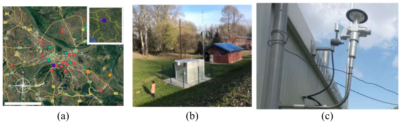
The air quality monitoring network in Belgrade (Figure 1a) is relatively dense, comprising 42 locations in total, of which ~36 are automatic monitoring sites. The majority (~30) are operated by the Institute of Public Health Belgrade (IPHB), with the remaining (~6) operated by the Serbian Environmental Protection Agency (SEPA). An additional 12 semi-automatic sites provide SO₂ and NO₂ measurements. Beyond online pollutant monitoring, selected sites support offline chemical analysis: PM10 samples are collected for heavy metals (HMs), PAHs, and saccharide tracers (levoglucosan, mannosan, galactosan), while PM2.5 samples are analyzed for OC/EC and ionic composition. The IPHB-operated stations collectively generate approximately ~4300 hourly averaged values per day. Supplementary measurements at a subset of stations include HM and B(a)P analysis at 10 locations (every second day), NO2, SO2 and soot at 10 locations (daily), and further HM monitoring at 20 locations (weekly) [32].
Within the framework of WeBaSOOP project, a pilot monitoring supersite was established at the Ada Marina, Belgrade automatic monitoring station, and it has been operational since June 2023. Figure 1a shows stations in Belgrade, including the Ada Marina automatic monitoring station, and Figure 1b shows the Ada Marina automatic monitoring station as seen from the outside. In addition to the standard set of air quality parameters typically present at the automatic monitoring station (SO2, NO, NO2, NOx, PM10, PM2.5, O3, CO, meteorological data), supersite features instruments for more comprehensive characterization of PM, namely: scanning mobility particle sizer (TSI 3082), condensation particle sizer (TSI 3775), optical particle size spectrometer (TSI 3330) and most relevant for this study filter absorption photometer (Magee AE33 aethalometer), capable of estimating real-time BC mass concentration and source apportionment differentiating between solid and liquid fuels [33]. Figure 1c shows the separate inlet for total carbon (TC) and black carbon (BC) measurements, which was added as a part of the pilot supersite infrastructure. In addition to these online measurement capable instruments, supersite features extensive gravimetric sampling for offsite laboratory analysis.
The Ada Marina pilot supersite is located in the largest sports and recreational area in the Belgrade central area, it is situated near the Sava River and surrounded by extensive green spaces (Figure 1a and Figure 1b). The local potential pollution sources include a number of nearby restaurants and a high-traffic arterial road, approximately 0,25 km away. Other local possible emission sources are: to the west, a natural gas residential heating plant (1,5 km), in the northwest, one of the busiest airports in the Balkan Peninsula, Belgrade “Nikola Tesla” Airport (~10 km). In addition to these sources, the international E-70 highway passes through Belgrade, however, it now primarily serves local transport, as the new Bypass encircles the city to handle transit traffic. Potential air pollution sources also include numerous smaller production plants and processing and storage facilities, along with diffused traffic from a wider Belgrade area.
Figure 1.
a) Network of automatic monitoring stations in Belgrade, traffic (red), background (green) and industrial sites (yellow), Ada Marina (blue), inset in the top right is showing Ada Marina, Belgrade location within Serbia, main map scale 10km, top of map faces North, b) outside of the Ada Marina, Belgrade supersite c) sampling inlet detail for black carbon and total carbon instruments.
Figure 1.
a) Network of automatic monitoring stations in Belgrade, traffic (red), background (green) and industrial sites (yellow), Ada Marina (blue), inset in the top right is showing Ada Marina, Belgrade location within Serbia, main map scale 10km, top of map faces North, b) outside of the Ada Marina, Belgrade supersite c) sampling inlet detail for black carbon and total carbon instruments.
The dataset obtained by combining the standard set of air quality parameters and additional parameters provided by the pilot supersite infrastructure can be used to prepare training and validation data for the virtual sensor model. Here only a limited subset of the complete dataset is used for finding possible predictors (a total of 11), since the goal is to derive a multilinear regression model for BC concentration estimation that can be potentially generalized and transfered to different sites within Belgrade area. Some of the predictors such as size resolved number concentration are omitted, by design, due to data availability and the limitations that the use of these advanced metrics would put on the potential model transfer.
Virtual BC Sensor Regression Models
Recently, a concept of virtual or soft sensors has been introduced [21] as a way of increasing spatial resolution by utilizing low-cost sensors and statistical concepts. By using a similar research vision, but instead of low-cost sensors [34] using high quality inputs from the reference station Ada Marina, Belgrade (Figure 1), we expand the concept of virtual sensors to reference air quality automatic monitoring networks, and determine to which extent it would be possible, in principle, to gain information about BC mass concentration based on statistical relationship with other pollutants. While a significant portion of previous studies [21,34] have used low-cost sensors as the main data source, in this study, only the measurements from the regulatory grade instruments are used for the development of the models. Some studies, such as [27] have also used measurements from regulatory grade instruments but models considered in this study only take into account predictor sets that are more readily available in traditional monitoring (such as NO2, PM2.5 mass concentration) thus making the models more easily deployable in a sensor network, like the one that exists in wider Belgrade area (Figure 1a). A virtual sensor that would require another rare sensor (e.g. a measurement from the condensation particle counter for particle number concentration, or even more complex size resolved number concentration [27]) would not be as easy to deploy as the one that uses more widely available regulatory data. There are several possible use cases for the virtual sensor approach. The virtual sensor model can be used to infer the missing data, and make BC concentration estimates for the automatic monitoring site, provided that the predictor variables for the virtual sensor model are available. Furthermore, if the pollution sources are similar, the virtual sensor model can also be transferred to another automatic monitoring site, and used there to infer the BC concentration. In this way the absence of the specialized instrumentation can be remedied, to some extent, and instead of directly relying on physical on-site sensor hardware one can utilize a relatively simple statistical model to estimate the BC concentration. This makes it possible to increase the spatial resolution for a virtualized air quality parameter, by applying it to several nodes of automatic monitoring sensor network.
In the context of air quality data analysis and modeling, one possible classification of the models is in terms of their explainability to the so called simpler "white-box" models, such as multiple linear regression models (MLRs) in which explainability is embedded by design, and to deep learning based "black-box" models, where such explainability is less obvious. These include random forests (RF), support vector regression (SVR), 1D convolutional neural networks (1D-CNN) and long short-term memory (LSTM) among others [27,35,36]. Note that this categorization is only based on immediate explainability of the models, and not on their performance in the specific context, since sometimes even simpler MLR approaches can outperform more complex machine learning methods in some respects. For example long term stability of multiple linear regression model can outperform random forest approach for low cost sensor calibration [37]. Furthermore, given that our datasets are relatively limited in size, deep learning models do not always outperform traditional machine learning techniques, such as MLR [38]. Specifically, for Black Carbon (BC) virtual sensing, "white-box" models, such as those based on linear regression, have been demonstrated to work effectively compared to "black-box" architectures like Long Short-Term Memory (LSTM) networks and other deep learning models [39]. Furthermore, research has shown that Bayesian linear regression [28] provides a powerful framework for modelling BC as a virtual sensor. Linear regression models are typically less prone to overfitting, more stable across multiple seasons or longer time spans, and allow comparatively straightforward interpretation of the model. For a use case studied in this paper, a classical regression problem, where the current sample of features is used to infer current sample of a target variable (point-wise mapping of features to targets), some of the aforementioned “black-box” models are inefficient. More specifically, 1D-CNNs lack the temporal dimension necessary for kernel convolution (since there is no time sequence for kernel to move through) and for LSTMs, similarly, there is no sequence to “remember”. Therefore, if choosing among ML models given above, more efficient machine learning approaches in our use case would be RF and SVR. Thus, in this study, the performance of regression models based on MLR, RF and SVR for BC sensor virtualization is explored in details.
MLR is a generalization of univariate linear regression, and after the choice of predictors in the linear model, it is straightforward to derive the modelling equation given by (1), for each data point in the training set i = 1, .., n:
which can be represented in a matrix form:
where X∙A is a system component, X containing predictor values for individual data points, A containing model parameters (to be determined in the process of training) and E is the residual. Model parameters are determined to minimize the residual sum of squares between the observed targets in the dataset:
The RF model is constructed by aggregating the outputs of multiple decision trees, each trained on different subsets of the data [35]. RF maintains strong predictive performance by reducing overfitting through ensemble averaging, which potentially enhances the model's generalization ability. This makes RF suitable for capturing the relationships between BC levels and the selected variables, even in the presence of noise or non-linear interactions. The RF regressor for the BC virtual sensors was implemented with 300 independent trees, where overfitting was mitigated by constraining the maximum tree depth to 5 and requiring a minimum of 10 samples per leaf node.
The Support Vector Machine (SVM) approach, introduced in [40], is a well-established statistical learning framework widely applied in air quality prediction, including BC concentration modeling [27]. Operating on the principle of regression, commonly referred to as Support Vector Regression (SVR) [41], the SVR optimization pursues a dual objective: identifying a function that deviates from the training outputs by no more than a specified threshold (ε), while simultaneously minimizing model complexity. A box constraint parameter C penalizes observations that exceed this margin, balancing model flatness against training error. The training points that fall on or outside the epsilon margin are termed support vectors, as they are the only points influencing the final regression fit. In this study, the SVR model for the BC virtual sensor employed a Radial Basis Function (RBF) kernel with the epsilon-insensitive margin set to 0.2, defining a tolerance zone within which prediction errors are not penalized. Constraint parameter C had a value of 1.0 providing a balance between fitting the training data well and keeping the model coefficients small [42].
The criteria for choosing the predictor variables is an important component of the model development, and here two approaches are used in the initial analysis. The first approach is (bottom up) stepwise linear regression [43]. Starting from the initial set of predictors (air quality variables that can be reasonably expected to be avaialable at any automatic monitoring network node) predictors are added one by one, based on the condition that they are most correlated with the residual from the previous step. Once there are negligible improvements of the adjusted R2, the step wise procedure is stopped and the set of predictors is concluded.
The second approach for the initial analysis of the predictors is based on adaptive best subset selection, using abess library [44]. Abess library implements a polynomial algorithm in the best-subset selection problem for the general linear regression, which minimizes mean squared error loss function subject to a constraint on the number of non-zero coefficients:
where is the norm, representing the count of non-zero elements in the coefficient vector, and s is number of non-zero elements (the sparsity level), which is either imposed or calculated by the abess algorithm.
A note about the fundamental difference between the two approaches for the choice of predictors is in place here. Stepwise linear regression approach, as described above, falls into the class of so called greedy algorithms [45], that is, algorithms that, as the name implies, make the locally optimal (greedy) choice at each step (in our case choose a predictor that has maximal correlation with the residual from the previous step), and after stopping criteria arrive at the solution that approximates or approaches the performance of the global optimum sufficiently well. Additionally, set of predictors in each step is only enlarged, i.e. sets are hierarchical in nature. On the other hand, abess algorithm is a non-greedy algorithm which maintains an active set of size s (the current best subset) and an inactive set of predictors (the remainder of the predictors). In each iteration it identifies a small number of predictors in the active set that contribute the least (and removes them from the active set) and replaces them with the same number of variables from the inactive set that would contribute the most. This process repeats until no further improvement is possible, is proven to run in polynomial time and often finds the exact global best subset for a fixed sparsity level [44].
In ordinary least squares regression – in contrast to orthogonal (or total) least squares – the predictors are assumed to be error-free, while all error is attributed to the dependent variable and is assumed to have constant variance (homoscedasticity). Given that the reference-grade instruments used here exhibit very low measurement error, this assumption is well justified. While approaches that handle errors in both independent and dependent variables (such as total least squares) are available, ordinary least squares is used due to its simplicity and practicality.
Since the Scikit-learn library [42] is utilized for the modeling, a training and validation split is employed for model validation and the estimation of predictive power. Extreme values were removed from the training set by removing the top and bottom percentiles of the target data, while no such trimming was performed on the test set. Rather than using the default random training-test split implemented in Scikit-learn, a sequential training-test split is applied, as this is more appropriate for time-series based modeling. Models developed and tested for sequential training and testing periods thus mimic real world deployment scenario – limited testing period followed by a long-term deployment.
3. Results
Correlation of Air Quality Parameters and Choice of Predictor Variables at the Supersite Ada Marina, Belgrade
The methods described above for the choice of predictors will now be applied. A stepwise calculation of the correlation matrix is required by the stepwise procedure, starting from the correlation matrix for the initial set of predictors, followed by additional rows for residuals in each of the steps. The investigation has been limited to 4 steps in the stepwise procedure. Air quality parameters used for calculation of correlation matrix depicted in Figure 2 are meteorological (pressure, temperature, relative humidity), gaseous pollutants (SO2, O3, NO, NO2, NOx, CO), particulate matter fractions (PM10, PM2.5) and aethalometer data (black carbon concentration derived using default mass absorption cross-section (MAC) values).
This correlation matrix can be used to guide the selection of predictor variables for the virtual sensor model, in a stepwise approach. Based on the BC column of the matrix, the strongest correlation is observed for NOx (0.90). In this first step residual is also calculated and enters the dataset, denoted as RES01. In the next iteration, the correlation of the remaining air quality variables with the residual RES01 is observed. After the most highly correlated predictor is chosen, the residual RES02 is again calculated, and this process is continued for subsequent steps. In the 4 step procedure the final set of predictors has 4 members: NOx, PM2.5, CO and O3. This initial analysis will only guide the choice of predictors, but results of statistical tools will also be critically considered using domain knowledge, and knowledge obtained from supersite analysis [46]. It is interesting to note that correlations that exist and can be observed in Figure 2 are in fact similar to those observed at several urban sites across Europe within RI-URBANS project in a study done by Fung et al. [27], performed in Barcelona, Helsinki and Dresden, featuring BC correlations with possible predictors (explanatory variables). In the class of predictors related to PM this study uses size resolved and total number concentration in the possible predictor sets, and have determined Pearson correlation in the range from 0.48 to 0.85. In our study predictors related to PM correlate with BC in the amount of 0.75 for PM2.5 and 0.59 for PM10. For O3, Fung et al study observed correlations -0.36 to -0.58, while our study found -0.57 (similar to Dresden urban site). Similarly, for NO2 Fung et al. found correlations in the range 0.69 – 0.85, while our study found 0.75 (again similar to Dresden urban site).
Coming back to our model, OLS derived equations for the BC concentration for the complete period are given by
where lefthand side is OLS estimate of BC mass concentration in stepwise linear regression procedure, going from 1 predictor () to 4 predictors (). This style of matrix notation is convenient since one can readily observe how value of parameters changes from iteration to iteration in the stepwise procedure, and also track the stability of the model. From Eq. 5 it is clear that the intercept, NOx and PM2.5 parameters are relatively stable throughout the iterations, while the CO varies more widely. Also, since the intercept is close to 0 in each of the 4 iterations, the model could be also calculated forcing the intercept to 0. Note however, that this initial analysis only serves to inform us about the possible choice of predictor set, and that the more robust derivation of model parameters will be done in the next section.
Figure 3.
a) Correlation matrix (Pearson correlation coefficient) between relevant air quality parameters and residuals in 4 step stepwise linear regression at the Ada Marina, Belgrade supersite during the non-heating season, calculated using 1-hour averages. Columns correspond to meteorological parameters (pressure, temperature, relative humidity), gaseous pollutants (SO2, O3, NO, NO2, NOx, CO), particulate matter fractions (PM2.5, PM10) and black carbon concentration. Remaining 4 columns RES01-RES04 correspond to the residuals in a 4-step stepwise procedure.
Figure 3.
a) Correlation matrix (Pearson correlation coefficient) between relevant air quality parameters and residuals in 4 step stepwise linear regression at the Ada Marina, Belgrade supersite during the non-heating season, calculated using 1-hour averages. Columns correspond to meteorological parameters (pressure, temperature, relative humidity), gaseous pollutants (SO2, O3, NO, NO2, NOx, CO), particulate matter fractions (PM2.5, PM10) and black carbon concentration. Remaining 4 columns RES01-RES04 correspond to the residuals in a 4-step stepwise procedure.
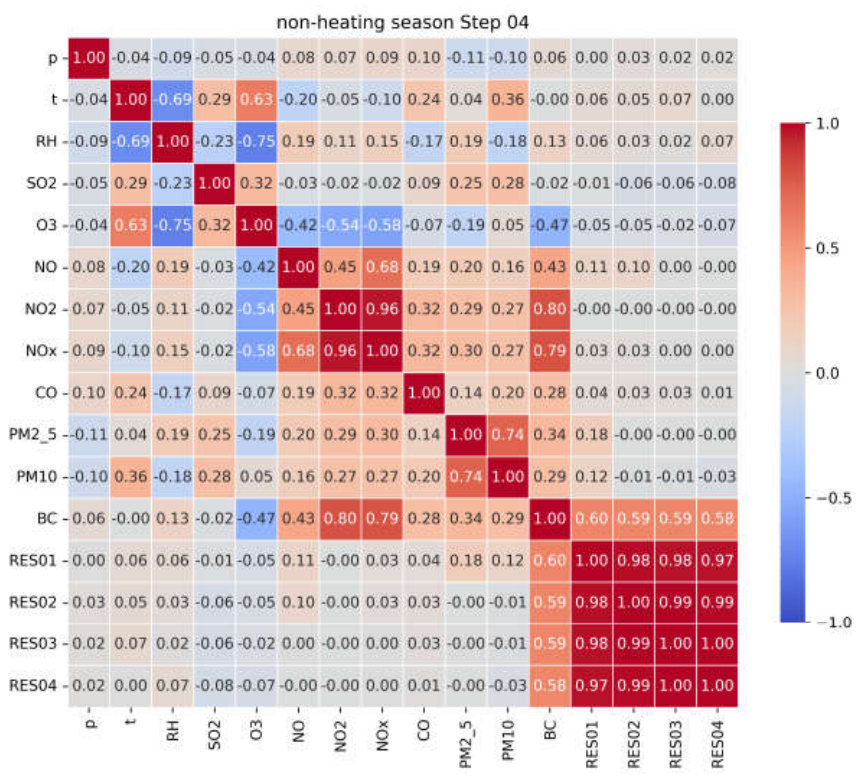
OLS derived equations for the BC concentration for the non-heating seasonare given by
Here it can be seen that the coefficients corresponding to first 3 predictors (NO2, PM2.5 and NO) are relatively stable throughout the stepwise procedure. Additionally, the intercept is close to zero, in all 4 iterations. This is in line with the physics based reasoning that the approximately zero concentration of gaseous products of combustion and approximately zero concentration of PM product of combustion will match with approxmately zero BC concentrations.
Figure 4.
a) Correlation matrix (Pearson correlation coefficient, unitless) between relevant air quality parameters and residuals in 4 step stepwise linear regression at the Ada Marina, Belgrade supersite during the heating season, calculated using 1-hour averages. Columns correspond to meteorological parameters (pressure, temperature, relative humidity), gaseous pollutants (SO2, O3, NO, NO2, NOx, CO), particulate matter fractions (PM2.5, PM10) and black carbon concentration. Remaining 4 columns RES01-RES04 correspond to the residuals in a 4-step stepwise procedure.
Figure 4.
a) Correlation matrix (Pearson correlation coefficient, unitless) between relevant air quality parameters and residuals in 4 step stepwise linear regression at the Ada Marina, Belgrade supersite during the heating season, calculated using 1-hour averages. Columns correspond to meteorological parameters (pressure, temperature, relative humidity), gaseous pollutants (SO2, O3, NO, NO2, NOx, CO), particulate matter fractions (PM2.5, PM10) and black carbon concentration. Remaining 4 columns RES01-RES04 correspond to the residuals in a 4-step stepwise procedure.
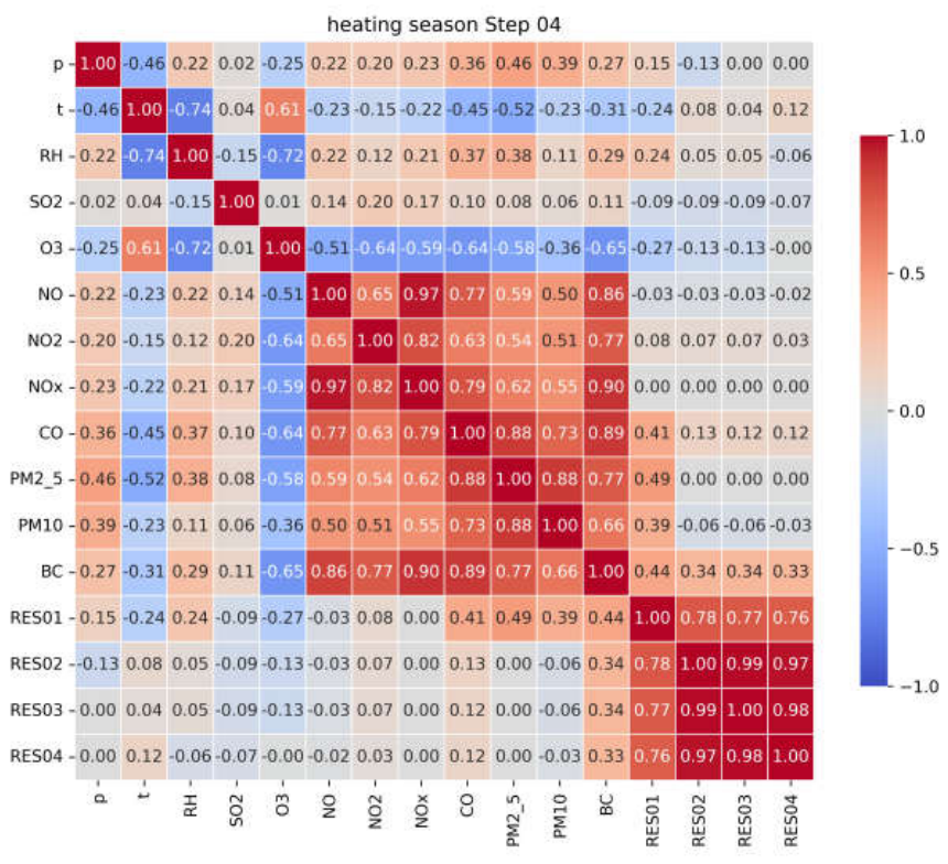
OLS derived equations for the BC concentration for the heating seasonare given by
In this case the coefficients corresponding to NOx and PM2.5 are very stable throughout the stepwise procedure; however, the intercept experiences the sudden increase with the introduction of non-pollutant meteorological predictor p. This sudden increase is to offset average pressure of around 1000 mbar as it cancels out with the coefficient corresponding to p (around – 0.0175 in Eq. 7).
It can be concluded that in all three training datasets (complete period, non-heating and heating season) nitrogen oxides play the role of the most descriptive predictor, followed by PM2.5 mass concentration. Additional predictors do not add much to the model, as can be seen from correlation between target BC concentration and residuals 3 and 4 (RES03 and RES04) in all 3 cases. Thus, the diversity of the predictors number 3 and number 4, can be considered as more of a mathematical artefact than some underlying air pollution related phenomena.
However, it should be also noted that stepwise regression does not always find the most optimal subset of predictors, since it is using a greedy algorithm. Thus, as a more robust alternative, which will complement initial analysis, the adaptive best subset selection, implemented in abess library [44], will be used for exploring possible subsets of up to 4 predictors. Since the air quality data is typically highly correlated, sparsity level from 1 to 4 is imposed in the abess algorithm, corresponding to models having from 1 to 4 predictors, thus avoiding the algorithm always choosing the maximum number of predictors (in studied case 11 predictors). The results are summarized in the table below.

Table 1.
Predictor set size and predictors for the complete period, non-heating season and heating season obtained using adaptive best subset selection.
Table 1.
Predictor set size and predictors for the complete period, non-heating season and heating season obtained using adaptive best subset selection.
| Predictor set size | Complete period | Non-heating season | Heating season |
|---|---|---|---|
| 1 | NOx | NO2 | NOx |
| 2 | NOx, PM2.5 | NO2, PM2.5 | NOx, CO |
| 3 | NOx, PM2.5, CO | NO2, PM2.5, p | NOx, CO, PM2.5 |
| 4 | NOx, PM2.5, CO, NO2 | NO2, PM2.5, p, NOx | NOx, CO, PM2.5, NO2 |
The scope of further testing will be limited to models with two predictor variables, as very similar conclusions regarding predictors have been reached using both the stepwise linear regression approach and adaptive best subset selection. Furthermore, models accuracy does not improve with additional predictors (more than 2 predictors) as can be observed from the residuals RES03 and RES04 in the correlation matrices and their correlation with the target BC concentration, which remains the same;
Table 2.
Virtual sensor models for further analysis based on the critical analysis of the stepwise linear regression approach and adaptive best subset selection.
Table 2.
Virtual sensor models for further analysis based on the critical analysis of the stepwise linear regression approach and adaptive best subset selection.
| Predictors | Complete period | Non-heating season | Heating season |
|---|---|---|---|
| 2 | NOx, PM2.5 | NO2, PM2.5 | NOx, CO |
| Same in stepwise and best subset approach? | Yes, both procedures give the same set of predictors when applied over the complete period. | Yes, both procedures give the same set of predictors when applied over the non-heating season period. It is also possible the use NOx as a predictor instead of NO2, since NO2 and NOx are very highly correlated at ~ 0.96 (see Figure 3) | No. Two procedures did not give the same set of predictors. Since abess is more robust, those predictors will be used. Stepwise model predictors derived from the heating season data are the same as for the complete period model |
Thus, the final virtual sensor MLR model equations are obtained:
The form of Eq. 8, can be explained by the fact that CO and nitrogen oxides are gaseous co-pollutants from similar combustion sources (especially traffic), CO is also present in the wood smoke, while PM2.5 includes BC as a major component. The RF and SVR models employ the same predictor-target configuration as the MLR model, however, given their algorithmic complexity, they cannot be expressed through a simple closed-form equation as is the case for MLR.
Training/Test Split Analysis of the Model Parameters and the Performance of the Virtual Sensor Models Onsite
Now that a set of predictors for the different seasons is established, it is possible to evaluate the performance of the virtual sensor models. The metrics that one can use are the same as the metrics typically used for real physical sensors, i.e. suitable metrics are R2 and RMSE as calculated on the test portion of the dataset.
It is well known that training and test split for the models based on time series should be performed in a sequential manner, see for example [47]. This also closely mimics real world scenarios of calibration of air monitoring devices, and similarly virtual sensor models, in which model data is collected for some time (training), and then model is tested (deployed) over prolonged periods of time. Table 3 summarizes first the performance of the MLR heating season models, where the training percentage (compared to the complete dataset) goes from 20% to 50% of a complete dataset in increments of 10%.
Similarly, Table 4 compares the performance of the MLR, RF and SVR based heating season models. Based on the results in Table 3 and Table 4 it is evident that using virtual sensor approach it is possible to achieve quite low values of RMSE, even for the heating season when the BC concentrations are much higher compared to the rest of the year, with RMSE going as low as 0.69 μg/m3 (MLR and RF models, 50/50 training test split). SVR model exhibits slightly worse performance, but still around ~1 μg/m3. The train/test splits (from 20/80 to 50/50) are mimicking the limited calibration data available in real-world AQ sensor deployment scenarios. Even with as little as 20% of data used for training, the models demonstrate strong generalization (MLR and RF models, R2 ~ 0.85), successfully predicting several months of previously unseen data. Table 3 also reflects how changes in training/test split influence the stability of the MLR model parameters. The benefits of simplicity and interpretability of the MLR model become immediately apparent when examining its coefficients across different train/test splits. The intercept remains consistently close to zero, suggesting physically sound model, while the NOx coefficient shows more stability compared to the CO coefficient – indicating that the relationship between NOx and BC concentrations is more robustly captured even when the model is trained on limited data. Note that this was also the result of the stepwise procedure in the previous subsection. Figure 5 shows all virtual sensor models performance for the heating season. Figure 5a show scatter plots of hourly values, and this is the data that was used for model training and testing (in a 50/50 sequential chronological split). This visual representation allows for a straightforward assessment of model performance, including any degradation on the test set and the representativity of the training data. Here the training and test set performance of the model are in almost perfect agreement, suggesting that no overfitting occurred, since all models generalize well on unseen data and have similar RMSE and R2 during training and test. This is also evident from the trendlines between virtual sensor and reference for all 3 models (inset in Figure 5a), where coefficients are very similar between train and test periods. Figure 5b shows 24h averages, where traces of predicted data and true data are very close (RMSE values for different periods are given in Figure 5a inset), for all 3 virtual sensor models approaches.
Table 5 summarizes the performance of the MLR non-heating season models, where the training percentage (compared to the non-heating season dataset) goes from 20% to 50% of a complete non-heating season dataset in increments of 10%. Non-heating season features much lower concentrations of BC, compared to the heating season, thus RMSE shown in Table 5, although similar in value to the RMSE of the heating season models is in terms of relative RMSE much higher than the one in the heating season model. However, the non-heating season models still perform very well, and have very stable linear regression parameters, not depending much on the training/test split, although the explained variance R2 is smaller than for the heating season models (~0.6 compared to ~0.9). Table 6 compares the performance of MLR, RF and SVR models. MLR and RF models again have very similar performance, while SVR has slightly lower R2 and slightly higher RMSE, compared to the other two. Figure 6 shows all virtual sensor models performance for the non-heating season. Figure 6a show scatter plots of hourly values, and this is the data that was used for model training and testing (in a 50/50 sequential chronological split). Right panel in Figure 6a shows presence of outliers, with high true BC concentration which isn’t registered in the models, which reduced the R2 and increases the RMSE compared to the training period. Figure 6b shows 24h averages, where it is evident that the daily concentration averages are much smaller compared to the heating season averages (maximal values are around 2.5 μg/m3, while during heating season they were around 10 μg/m3). While the RMSE is similar for both heating and non-heating season models in most cases (ranging from 0.6 to 1.2 μg/m3), during the non-heating season overall BC concentrations are much lower, resulting in the substantial reduction of the explained variance. Traces of predicted data and true data are still very close, but also one can notice the size of relative errors which are larger than those that can be seen in Figure 5b. Additional explanation for lower performance of the non-heating season model could be sought in the drastic changes in carbonaceous aerosols composition going from heating season into the non-heating season. As reported in [46] during the period of the study at the Belgrade pilot supersite fossil fuel (traffic) contributions show little seasonality, while residential wood combustion (RWC) drops from being overly dominant in winter to almost non existing in summer. Furthermore, in spring/summer, carbonaceous aerosol is dominated by biogenic secondary organic aerosols (BSOA) and primary biological aerosol particles (PBAP) at more than 20% of carbonaceous aerosol, neither of which contributes to a BC signal.
Finaly, Table 7 summarizes the performance of the MLR complete period models, where the training percentage (compared to the complete period dataset) goes from 20% to 50%, in the increments of 10%. Note here, that the training data is chosen from the first half of the data, mostly consisting of heating season data. However, the virtual sensor models still perform quite well but the drop in R2 is evident, compared to the specialized heating season models. This can be explained in the following manner. The overall span of air quality parameters for which the models are constructed will need to sufficiently capture the conditions in which models will be used, otherwise performance drops of the models are to be expected. The gradual drop in R2 observed in Table 7 occurs because, as the training set expands, the test set ceases to be sufficiently representative. Specifically, the test set lacks the higher Black Carbon (BC) values characteristic of the heating season, which are absent during the non-heating season. Additionally, the MLR intercept is close to zero, in all considered models, and for all training/test splits. This is in line with the physics-based reasoning that the approximately zero concentration of gaseous products of combustion and approximately zero concentration of PM product of combustion will match with approximately zero BC concentrations. Table 8 compares the performance of MLR, RF and SVR models. It can be seen that in contrast to the specialized heating/non-heating season models, for the complete period all training/test splits, for all models, give only 1-2% difference in R2. Therefore, having in mind large differences in the complexity of the models, one can argue that most simple model that yields comparable results is most effective, this being the MLR model. Figure 7a shows scatter plot of hourly values, and this is the data that was used for model training and testing of the complete period models (in a 50/50 sequential chronological split). Figure 7b shows 24h averages. Traces of predicted data and true data are very close, clearly illustrating the good performance of the models. This figure also illustrates the power of virtual sensor approach, where a simple linear model, using only inputs that are a part of traditional regulatory monitoring can match really well with the BC signal coming from a dedicated reference instrument.
A note about predictors for cases of heating, non-heating and complete period is in place here. For the heating season (predictors are NOx and CO), the virtual sensor models achieve outstanding performance, with R2 ~ 0.94. There is no PM2.5 in the feature set, instead CO is used, which is a direct combustion tracer co-emitted with BC from both RWC and traffic. This makes physical sense since in winter in Belgrade [46], RWC dominates carbonaceous aerosol and thus CO tracks combustion intensity better than PM2.5 mass. For the non-heating season (predictors are NO₂ and PM2.5), the reduced performance of the models with R² ~ 0.6 can be explained by the fact that the overall BC concentrations are lower, thus noise is more pronounced, dominant sources that were very well explainable during heating-season are non-existent during summer, and furthermore PM2.5 also contains biogenic SOA, that does not contribute to the BC signal. Finally, for the complete period where predictors are NOx and PM2.5, the model contains both the traffic proxies (NOx) and total combustion mass PM2.5, thus, in a way, averaging over seasonal source shifts.
Regarding the transferability of the models, first step is to determine if the predictors for the desired BC virtual sensor are available at the transfer site. Here the complete period model has very suitable and generally available predictors, namely NOx and PM2.5, that exist in almost all nodes in Belgrade sensor network. From the total of 27 stations from the local Belgrade network being operational during time of the study all have the needed predictors, and from the 3 stations in the state network at the territory of Belgrade only one is missing PM2.5. Going further, specialized heating season model (NOx and CO predictors) uses CO data signal, which is not readily available in the whole network, 5 out of 27 operational stations during the study period do not have this signal, and only 1 out of 3 stations in the state network has both predictor signals. Finally, for the non-heating season model (NO2, PM2.5 predictors) 2 out of 3 stations from the state network at the territory of Belgrade have the needed predictors, and all 27 local Belgrade network nodes have the needed predictors. Formal validation of model transfer to other network nodes would require targeted measurement campaigns with offline EC analysis. Nevertheless, it is reasonable to expect that sites with an urban background source configuration similar to Ada Marina would yield comparable model performance, and this is identified as a priority direction for future work. In this context, it is worth noting that within the EU-funded RI-URBANS project, BC virtual sensor models trained in Barcelona were successfully validated in Helsinki and Dresden, achieving R² in the range 0.79–0.86, but without seasonal aggregation of data [27]. RI-URBANS methodologies have been referenced in the context of the recent revision of the European Air Quality Directive, which introduces BC monitoring requirements, further supporting the relevance of virtual sensing as a modeling approach for BC. The models developed in this study achieve R² up to 0.94 for the heating season and approximately 0.70 for the complete period on unseen data, representing a meaningful contribution to BC monitoring capacity in Belgrade and a foundation for broader network-level application.
4. Conclusions
In this paper three different virtual sensor models for black carbon mass concentration in ambient air are explored. Models are using the data from a Belgrade supersite as a target, and input data that is widely available in the air quality automatic monitoring station network. Predictors for the models were determined by two complementary methods, namely, greedy stepwise linear regression method, and non-greedy algorithm based on adaptive best subset selection. Predictors for BC included CO and nitrogen oxides as well as PM2.5. It was shown that for a variety of sequential training/test periods, the best performing models for the different periods were the following. For the heating season MLR and RF with R2 ~ 0.85–0.94, RMSE ~ 0.65–1.18 μg/m3, for the non-heating season, again MLR and RF with R2 ~ 0.59 – 0.61, RMSE ~ 0.80 – 0.88 μg/m3, and for the complete period all models, including SVR, exhibit similar performance with R2 ~ 0.70 – 0.87, RMSE ~ 0.74 – 1.03 μg/m3. This approach, carefully applied and taking into account local predictors configuration, paves the way for black carbon mass concentration estimates on sensor network sites with no dedicated black carbon measuring instruments, and useful modeling application for the BC emerging pollutant. Data for this study was collected at the newly-established pilot supersite located at the automatic monitoring station Ada Marina, Belgrade, making this modelling application on BC sensor virtualization first of its kind in this urban area and can help in filling in the gap that exists in air quality knowledge in this part of Europe.
Author Contributions
Conceptualization, M.D.; methodology, M.D. and M.D.; software, M.D.; validation, M.D., M.D., D.B.S; formal analysis, M.D.; investigation, M.D. and M.D; resources, M.D, D.B.S, M.J.-S., A.Š;; data curation, M.D, D.B.S, M.J.-S., A.Š; writing—original draft preparation, M.D; writing—review and editing, all authors; visualization, M.D, and M.D; supervision, M.J.-S.; project administration, M.D., M.J.-S.; funding acquisition, M.J.-S. and T.S. All authors have read and agreed to the published version of the manuscript.
Funding
This work was funded by European Union’s Horizon Europe Research and Innovation Program under GA 101060170 (WeBaSOOP project https://webasoop.org), the project 22DIT02 FunSNM (https://www.funsnm.eu/) has received funding from the European Partnership on Metrology, co-financed from the European Union’s Horizon Europe Research and Innovation Programme and by the Participating States; and the Ministry of Science, Technological Development and Innovation of the Republic of Serbia under GA 451-03-136/2025-03/200017.
Data Availability Statement
Research data used for this study is largely the result of the WeBaSOOP project. Links to the relevant data can be found at https://webasoop.org/ and will be active after the embargo period. The data from the automatic reference monitoring stations is available in real time at https://sepa.gov.rs/ (national monitoring network) and https://www.beoeko.com/ (local Belgrade monitoring network).
Abbreviations
The following abbreviations are used in this manuscript:
| EEA | European Environment Agency |
| AAQD | European Ambient Air Quality Directive |
| IARC | International Agency for Research on Cancer |
| RMSE | Root mean square error |
| BC | Black Carbon |
| OC | Organic Carbon |
| EC | Elemental Carbon |
| PM | Particulate Matter |
| eBC | equivalent Black Carbon |
| MLR | Multiple Linear Regression |
| RF | Random Forest |
| SVR | Support Vector Regression |
| abess | adaptive best subset selection |
References
- Agency, E.E. Europe's environment 2025 – Knowledge for resilience, prosperity and sustainability; Publications Office of the European Union: 2025.
- Straif, K.; Cohen, A.; Samet, J. Air pollution and Cancer; International Agency for Research on Cancer (IARC) / World Health Organization: Lyon, France, 2013.
- BELIS, C.; KONA, A.; THUNIS, P.; PISONI, E.; ZAULI, S.S.; DE, M.; REY, P.A.; PEKAR, F. Urban PM2. 5 Atlas. Air Quality in Cities of Countries involved in the EU Enlargement policy.
- THUNIS, P.; PISONI, E.; ZAULI, S.S.; DE, M.; REY, P.A.; PEKAR, F. Urban PM2. 5 Atlas Air Quality in European Cities, 2025 Report; 2023.
- European, P.; Council of the European, U. Directive 2008/50/EC of the European Parliament and of the Council of 21 May 2008 on ambient air quality and cleaner air for Europe. Official Journal of the European Union 2008, L, 1–44.
- World Health, O. Air quality guidelines: global update 2005: particulate matter, ozone, nitrogen dioxide and sulfur dioxide; World Health Organization. Regional Office for Europe: 2006.
- Adães, J.; Pires, J.C. Analysis and modelling of PM2. 5 temporal and spatial behaviors in European cities. Sustainability 2019, 11, 6019. [CrossRef]
- Saraga, D.; Maggos, T.; Degrendele, C.; Klánová, J.; Horvat, M.; Kocman, D.; Kanduč, T.; Dos Santos, S.G.; Franco, R.; Gómez, P.M. Multi-city comparative PM2. 5 source apportionment for fifteen sites in Europe: The ICARUS project. Science of the total Environment 2021, 751, 141855. [CrossRef]
- Liu, X.; Zhang, X.; Jin, B.; Wang, T.; Qian, S.; Zou, J.; Dinh, V.N.T.; Jaffrezo, J.-L.; Uzu, G.; Dominutti, P. Source apportionment of PM10 based on offline chemical speciation data at 24 European sites. npj climate and atmospheric science 2025, 8, 255. [CrossRef]
- Paisi, N.; Kushta, J.; Pozzer, A.; Violaris, A.; Lelieveld, J. Health effects of carbonaceous PM2. 5 compounds from residential fuel combustion and road transport in Europe. Scientific Reports 2024, 14, 1530. [CrossRef]
- Kelly, F.J.; Fussell, J.C. Size, source and chemical composition as determinants of toxicity attributable to ambient particulate matter. Atmospheric environment 2012, 60, 504–526. [CrossRef]
- Weichenthal, S.; Pinault, L.; Christidis, T.; Burnett, R.T.; Brook, J.R.; Chu, Y.; Crouse, D.L.; Erickson, A.C.; Hystad, P.; Li, C. How low can you go? Air pollution affects mortality at very low levels. Science Advances 2022, 8, eabo3381. [CrossRef]
- Liu, S.; Jørgensen, J.T.; Ljungman, P.; Pershagen, G.; Bellander, T.; Leander, K.; Magnusson, P.K.; Rizzuto, D.; Hvidtfeldt, U.A.; Raaschou-Nielsen, O. Long-term exposure to low-level air pollution and incidence of asthma: the ELAPSE project. European Respiratory Journal 2021, 57. [CrossRef]
- Organization, W.H. WHO global air quality guidelines: particulate matter (PM2. 5 and PM10), ozone, nitrogen dioxide, sulfur dioxide and carbon monoxide; World Health Organization: 2021.
- European, P.; Council of the European, U. Directive (EU) 2024/2881 of the European Parliament and of the Council of 23 October 2024 on ambient air quality and cleaner air for Europe. Official Journal of the European Union 2024.
- Janssen, N.A.; Gerlofs-Nijland, M.E.; Lanki, T.; Salonen, R.O.; Cassee, F.; Hoek, G.; Fischer, P.; Brunekreef, B.; Krzyzanowski, M. Health effects of black carbon; World Health Organization. Regional Office for Europe: 2012.
- Janssen, N.A.; Hoek, G.; Simic-Lawson, M.; Fischer, P.; Van Bree, L.; Ten Brink, H.; Keuken, M.; Atkinson, R.W.; Anderson, H.R.; Brunekreef, B. Black carbon as an additional indicator of the adverse health effects of airborne particles compared with PM10 and PM2. 5. Environmental health perspectives 2011, 119, 1691. [CrossRef]
- Novakov, T.; Rosen, H. The black carbon story: early history and new perspectives. Ambio 2013, 42, 840–851. [CrossRef]
- Savadkoohi, M.; Pandolfi, M.; Favez, O.; Putaud, J.-P.; Eleftheriadis, K.; Fiebig, M.; Hopke, P.K.; Laj, P.; Wiedensohler, A.; Alados-Arboledas, L. Recommendations for reporting equivalent black carbon (eBC) mass concentrations based on long-term pan-European in-situ observations. Environment international 2024, 185, 108553. [CrossRef]
- European Committee for, S. Ambient air - Measurement of elemental carbon (EC) and organic carbon (OC) collected on filters. 2017.
- Zaidan, M.A.; Motlagh, N.H.; Boor, B.E.; Lu, D.; Nurmi, P.; Petäjä, T.; Ding, A.; Kulmala, M.; Tarkoma, S.; Hussein, T. Virtual SenSorS: toward HigH-reSolution air pollution monitoring uSing ai and iot. IEEE Internet of Things Magazine 2023, 6, 76–81. [CrossRef]
- Domènech-Gil, G.; Puglisi, D. Benefits of virtual sensors for air quality monitoring in humid conditions. Sensors and Actuators B: Chemical 2021, 344, 130294. [CrossRef]
- Zaidan, M.A.; Motlagh, N.H.; Fung, P.L.; Lu, D.; Timonen, H.; Kuula, J.; Niemi, J.V.; Tarkoma, S.; Petäjä, T.; Kulmala, M. Intelligent calibration and virtual sensing for integrated low-cost air quality sensors. IEEE Sensors Journal 2020, 20, 13638–13652. [CrossRef]
- Kusiak, A.; Li, M.; Zheng, H. Virtual models of indoor-air-quality sensors. Applied Energy 2010, 87, 2087–2094.
- Leidinger, M.; Sauerwald, T.; Reimringer, W.; Ventura, G.; Schütze, A. Selective detection of hazardous VOCs for indoor air quality applications using a virtual gas sensor array. Journal of Sensors and Sensor systems 2014, 3, 253–263. [CrossRef]
- Tabandeh, S.; Vedurmudi, A.P.; Söderblom, H.; Pourjamal, S.; Harris, P.; Luo, Y.; Gruber, M.; Vaa, M.; Johansen, M.; Koval, M. Sensor network metrology: Current state and future directions. Measurement: Sensors 2025, 38, 101798. [CrossRef]
- Fung, P.L.; Savadkoohi, M.; Zaidan, M.A.; Niemi, J.V.; Timonen, H.; Pandolfi, M.; Alastuey, A.; Querol, X.; Hussein, T.; Petäjä, T. Constructing transferable and interpretable machine learning models for black carbon concentrations. Environment international 2024, 184, 108449. [CrossRef]
- Zaidan, M.A.; Wraith, D.; Boor, B.E.; Hussein, T. Bayesian proxy modelling for estimating black carbon concentrations using white-box and black-box models. Applied sciences 2019, 9, 4976. [CrossRef]
- D’Elia, G.; Ferro, M.; Sommella, P.; Ferlito, S.; De Vito, S.; Di Francia, G. Concept drift mitigation in low-cost air quality monitoring networks. Sensors 2024, 24, 2786. [CrossRef]
- European, C. WeBaSOOP: Research Reinforcing in the Western Balkans in Offline and Online Monitoring and Source Identification of Atmospheric Particles. 2022. [CrossRef]
- Serbian Environmental Protection, A. SEPA: Real-time Air Quality Monitoring Data Portal. 2026.
- Šoštarić, A.; Cvetković, A. Air Quality Monitoring in the City of Belgrade. In Proceedings of the Abstracts of Keynote Invited Lectures and Contributed Papers, The Tenth WeBIOPATR Workshop & Conference – Particulate Matter: Research and Management (WeBIOPATR 2025), Belgrade, Serbia, 2025/11/26, 2025.
- Sandradewi, J.; Prévôt, A.S.; Weingartner, E.; Schmidhauser, R.; Gysel, M.; Baltensperger, U. A study of wood burning and traffic aerosols in an Alpine valley using a multi-wavelength Aethalometer. Atmospheric Environment 2008, 42, 101–112. [CrossRef]
- Ferrer-Cid, P.; Paredes-Ahumada, J.; Barcelo-Ordinas, J.M.; Garcia-Vidal, J. Virtual sensor-based proxy for black carbon estimation in IoT platforms. Internet of Things 2024, 27, 101284. [CrossRef]
- Yu, R.; Yang, Y.; Yang, L.; Han, G.; Move, O.A. RAQ–A random forest approach for predicting air quality in urban sensing systems. Sensors 2016, 16, 86. [CrossRef]
- Ragab, M.G.; Abdulkadir, S.J.; Aziz, N.; Al-Tashi, Q.; Alyousifi, Y.; Alhussian, H.; Alqushaibi, A. A novel one-dimensional CNN with exponential adaptive gradients for air pollution index prediction. Sustainability 2020, 12, 10090. [CrossRef]
- De Vito, S.; Del Giudice, A.; D’Elia, G.; Esposito, E.; Fattoruso, G.; Ferlito, S.; Formisano, F.; Loffredo, G.; Massera, E.; D’Auria, P. Future low-cost urban air quality monitoring networks: insights from the EU’s AirHeritage project. Atmosphere 2024, 15, 1351. [CrossRef]
- Sabo, F.; Meroni, M.; Waldner, F.; Rembold, F. Is deeper always better? Evaluating deep learning models for yield forecasting with small data. Environmental Monitoring and Assessment 2023, 195, 1153. [CrossRef]
- Fung, P.L.; Zaidan, M.A.; Timonen, H.; Niemi, J.V.; Kousa, A.; Kuula, J.; Luoma, K.; Tarkoma, S.; Petäjä, T.; Kulmala, M. Evaluation of white-box versus black-box machine learning models in estimating ambient black carbon concentration. Journal of aerosol science 2021, 152, 105694. [CrossRef]
- Stitson, M.; Weston, J.; Gammerman, A.; Vovk, V.; Vapnik, V. Theory of support vector machines. University of London 1996, 117, 188–191.
- Awad, M.; Khanna, R. Support vector regression. In Efficient learning machines: Theories, concepts, and applications for engineers and system designers; Springer: 2015; pp. 67–80.
- Pedregosa, F.; Varoquaux, G.; Gramfort, A.; Michel, V.; Thirion, B.; Grisel, O.; Blondel, M.; Prettenhofer, P.; Weiss, R.; Dubourg, V. Scikit-learn: Machine learning in Python. the Journal of machine Learning research 2011, 12, 2825–2830.
- Efroymson, M. Stepwise regression–a backward and forward look. In Proceedings of the Eastern Regional Meetings of the Institute of Mathematical Statistics, 1966; pp. 27–29.
- Zhu, J.; Wang, X.; Hu, L.; Huang, J.; Jiang, K.; Zhang, Y.; Lin, S.; Zhu, J. abess: a fast best-subset selection library in python and R. Journal of Machine Learning Research 2022, 23, 1–7.
- Black, P.E. greedy algorithm. Dictionary of Algorithms and Data Structures.
- Petrović, B.; Živković, M.; Jovanović, M.; Davidović, M.; Platt, S.M.; Yttri, K.E.; Bartonova, A.; Jovašević-Stojanović, M. Distinguishing between anthropogenic and natural sources of carbonaceous aerosol in Belgrade. In Proceedings of the 3rd International Annual Belgrade Environmental Pollution Conference (IABEP 2025) - Book of Abstracts, Belgrade, Serbia, 2025/10/13, 2025.
- De Vito, S.; D’Elia, G.; Ferlito, S.; Di Francia, G.; Davidović, M.D.; Kleut, D.; Stojanović, D.; Jovaševic-Stojanović, M. A global multiunit calibration as a method for large-scale IoT particulate matter monitoring systems deployments. IEEE Transactions on Instrumentation and Measurement 2023, 73, 1–16. [CrossRef]
Figure 2.
Correlation matrix (Pearson correlation coefficient) between relevant air quality parameters and residuals in 4 step stepwise linear regression at the Ada Marina, Belgrade supersite during the complete period between October 21st 2023 to August 19th 2024, calculated using 1-hour averages. Columns correspond to meteorological parameters (pressure, temperature, relative humidity), gaseous pollutants (SO2, O3, NO, NO2, NOx, CO), particulate matter fractions (PM2.5, PM10) and black carbon concentration. Remaining 4 columns RES01-RES04 correspond to the residuals in a 4-step stepwise procedure.
Figure 2.
Correlation matrix (Pearson correlation coefficient) between relevant air quality parameters and residuals in 4 step stepwise linear regression at the Ada Marina, Belgrade supersite during the complete period between October 21st 2023 to August 19th 2024, calculated using 1-hour averages. Columns correspond to meteorological parameters (pressure, temperature, relative humidity), gaseous pollutants (SO2, O3, NO, NO2, NOx, CO), particulate matter fractions (PM2.5, PM10) and black carbon concentration. Remaining 4 columns RES01-RES04 correspond to the residuals in a 4-step stepwise procedure.
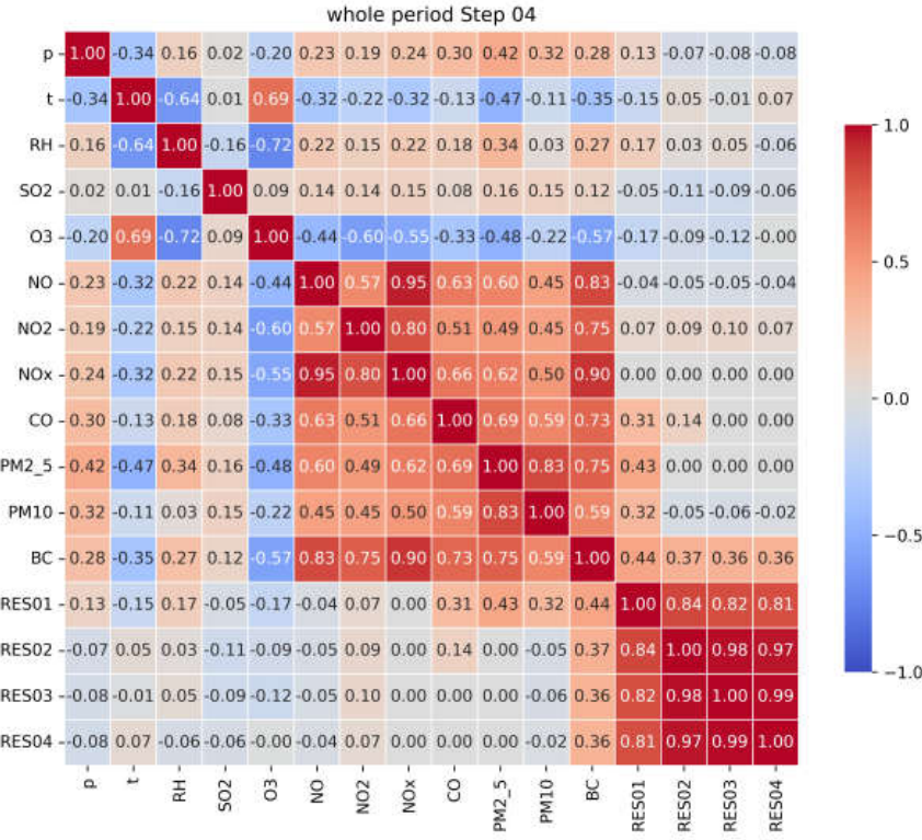
Figure 5.
True vs predicted equivalent BC values [μg/m3], using the MLR, RF and SVR virtual sensor models for the heating season and 50/50 training/test split a) scatter plot of hourly values with summary statistics for the training and test set b) time series of 24-hour averages.
Figure 5.
True vs predicted equivalent BC values [μg/m3], using the MLR, RF and SVR virtual sensor models for the heating season and 50/50 training/test split a) scatter plot of hourly values with summary statistics for the training and test set b) time series of 24-hour averages.
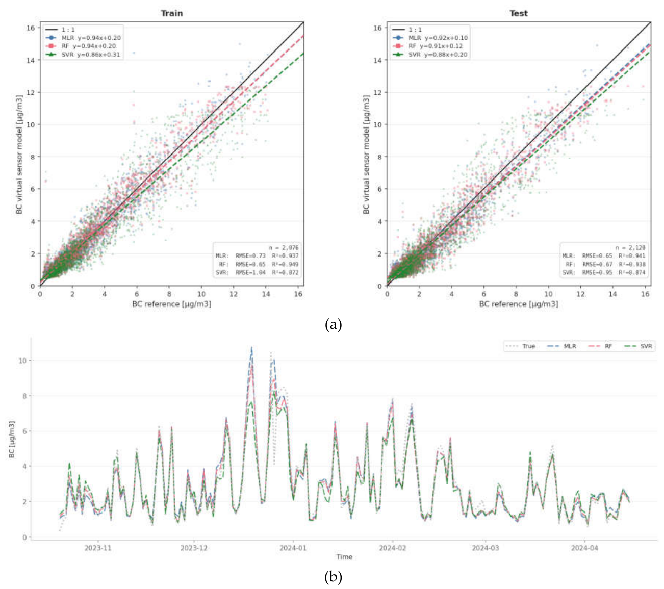
Figure 6.
True vs predicted equivalent BC values [μg/m3], using the MLR, RF and SVR virtual sensor models for the non-heating season and 50/50 training/test split a) scatter plot of hourly values with summary statistics for the training and test set b) time series of 24-hour averages.
Figure 6.
True vs predicted equivalent BC values [μg/m3], using the MLR, RF and SVR virtual sensor models for the non-heating season and 50/50 training/test split a) scatter plot of hourly values with summary statistics for the training and test set b) time series of 24-hour averages.
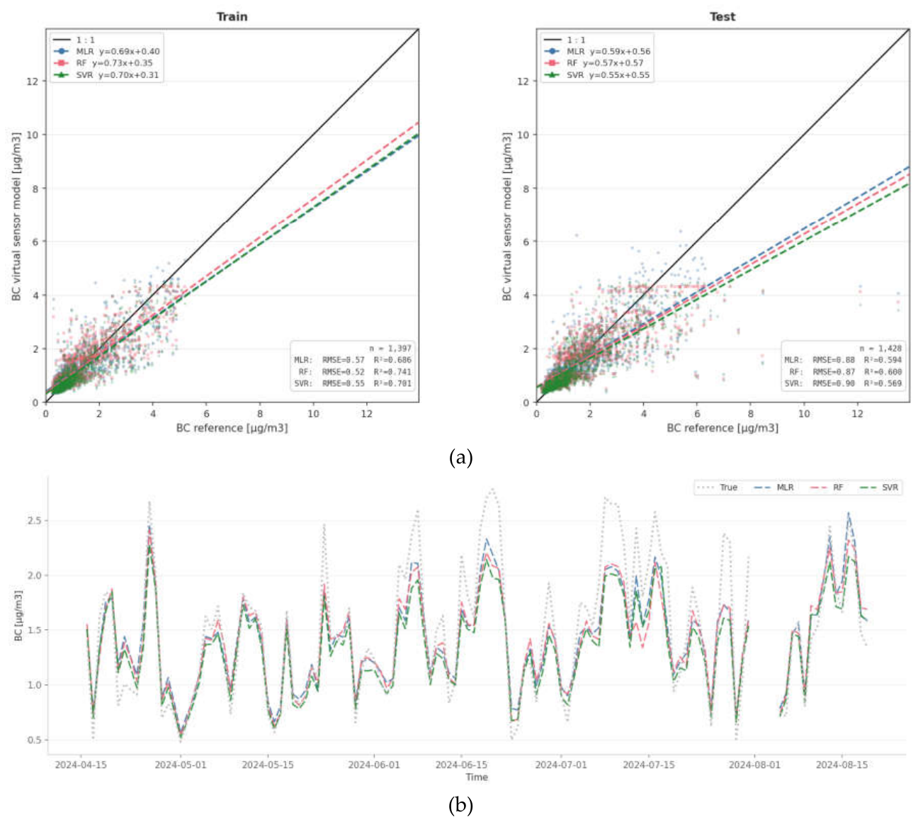
Figure 7.
True vs predicted equivalent BC values [μg/m3], using the MLR, RF and SVR virtual sensor models for the complete period and 50/50 training/test split a) scatter plot of hourly values with summary statistics for the training and test set b) time series of 24-hour averages.
Figure 7.
True vs predicted equivalent BC values [μg/m3], using the MLR, RF and SVR virtual sensor models for the complete period and 50/50 training/test split a) scatter plot of hourly values with summary statistics for the training and test set b) time series of 24-hour averages.
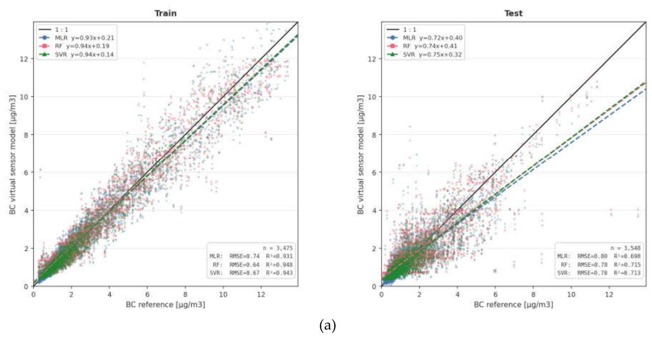
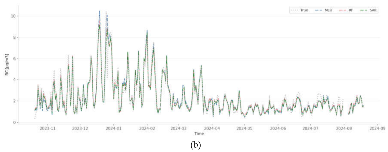
Table 3.
Performance of the MLR virtual sensor model Eq. (8) for the heating season depending on the training and test split, . All reported performance metrics are calculated using the test set.
Table 3.
Performance of the MLR virtual sensor model Eq. (8) for the heating season depending on the training and test split, . All reported performance metrics are calculated using the test set.
| Training/ test |
R2 | RMSE [μg/m3] | |||
| 20/80 | 0.8760 | 1.0782 | 0.0358 | 4.0989 | 0.1334 |
| 30/70 | 0.8694 | 1.1390 | 0.0379 | 3.1961 | 0.0918 |
| 40/60 | 0.9380 | 0.6661 | 0.0317 | 4.3067 | 0.1261 |
| 50/50 | 0.9408 | 0.6507 | 0.0318 | 4.2772 | 0.1612 |
Table 4.
Comparison of MLR, RF and SVR approach for the BC virtual sensor for the heating season depending on the training and test split. All 3 models of the virtual sensor use NOx and CO as input features. All reported performance metrics are calculated using the test set.
Table 4.
Comparison of MLR, RF and SVR approach for the BC virtual sensor for the heating season depending on the training and test split. All 3 models of the virtual sensor use NOx and CO as input features. All reported performance metrics are calculated using the test set.
| MLR | RF | SVR | ||||
|---|---|---|---|---|---|---|
| Training/ test |
R2 | RMSE [μg/m3] | R2 | RMSE [μg/m3] | R2 | RMSE [μg/m3] |
| 20/80 | 0.8760 | 1.0782 | 0.8545 | 1.1680 | 0.7474 | 1.5392 |
| 30/70 | 0.8694 | 1.1390 | 0.8597 | 1.1806 | 0.7427 | 1.5987 |
| 40/60 | 0.9380 | 0.6661 | 0.9343 | 0.6861 | 0.8637 | 0.9879 |
| 50/50 | 0.9408 | 0.6507 | 0.9381 | 0.6654 | 0.8742 | 0.9491 |
Table 5.
Performance of the MLR virtual sensor model Eq. (8) for the non-heating season depending on the training and test split, . All reported performance metrics are calculated using the test set.
Table 5.
Performance of the MLR virtual sensor model Eq. (8) for the non-heating season depending on the training and test split, . All reported performance metrics are calculated using the test set.
| Training/ test |
R2 | RMSE [μg/m3] | |||
| 20/80 | 0.6065 | 0.8051 | 0.0538 | 0.0354 | -0.0878 |
| 30/70 | 0.5919 | 0.8451 | 0.0513 | 0.0343 | -0.0136 |
| 40/60 | 0.5937 | 0.8674 | 0.0524 | 0.0313 | 0.0343 |
| 50/50 | 0.5943 | 0.8751 | 0.0546 | 0.0236 | 0.1127 |
Table 6.
Comparison of MLR, RF and SVR approach for the BC virtual sensor for the non-heating season depending on the training and test split. All 3 models of the virtual sensor use NO2 and PM2.5 as input features. All reported performance metrics are calculated using the test set.
Table 6.
Comparison of MLR, RF and SVR approach for the BC virtual sensor for the non-heating season depending on the training and test split. All 3 models of the virtual sensor use NO2 and PM2.5 as input features. All reported performance metrics are calculated using the test set.
| MLR | RF | SVR | ||||
|---|---|---|---|---|---|---|
| Training/ test |
R2 | RMSE [μg/m3] | R2 | RMSE [μg/m3] | R2 | RMSE [μg/m3] |
| 20/80 | 0.6065 | 0.8051 | 0.6004 | 0.8113 | 0.5681 | 0.8435 |
| 30/70 | 0.5919 | 0.8451 | 0.5935 | 0.8434 | 0.5586 | 0.8789 |
| 40/60 | 0.5937 | 0.8674 | 0.6033 | 0.8571 | 0.5540 | 0.9088 |
| 50/50 | 0.5943 | 0.8751 | 0.5999 | 0.8691 | 0.5688 | 0.9022 |
Table 7.
Performance of the virtual sensor model Eq. (8) for the complete period depending on the training and test split, . All reported performance metrics are calculated using the test set.
Table 7.
Performance of the virtual sensor model Eq. (8) for the complete period depending on the training and test split, . All reported performance metrics are calculated using the test set.
| Training/ test percentage |
R2 | RMSE [μg/m3] | |||
| 20/80 | 0.8417 | 1.0075 | 0.0411 | 0.0508 | -0.0592 |
| 30/70 | 0.8603 | 0.7785 | 0.0394 | 0.0560 | -0.1043 |
| 40/60 | 0.7708 | 0.7701 | 0.0384 | 0.0561 | -0.1044 |
| 50/50 | 0.6981 | 0.7982 | 0.0388 | 0.0552 | -0.1741 |
Table 8.
Comparison of MLR, RF and SVR approach for the BC virtual sensor for the complete period depending on the training and test split. All 3 models of the virtual sensor use NOx and PM2.5 as input features. All reported performance metrics are calculated using the test set.
Table 8.
Comparison of MLR, RF and SVR approach for the BC virtual sensor for the complete period depending on the training and test split. All 3 models of the virtual sensor use NOx and PM2.5 as input features. All reported performance metrics are calculated using the test set.
| MLR | RF | SVR | ||||
|---|---|---|---|---|---|---|
| Training/ test |
R2 | RMSE [μg/m3] | R2 | RMSE [μg/m3] | R2 | RMSE [μg/m3] |
| 20/80 | 0.8417 | 1.0075 | 0.8495 | 0.9824 | 0.8334 | 1.0337 |
| 30/70 | 0.8603 | 0.7785 | 0.8723 | 0.7443 | 0.8744 | 0.7382 |
| 40/60 | 0.7708 | 0.7701 | 0.7830 | 0.7493 | 0.7887 | 0.7394 |
| 50/50 | 0.6981 | 0.7982 | 0.7154 | 0.7750 | 0.7128 | 0.7786 |
Disclaimer/Publisher’s Note: The statements, opinions and data contained in all publications are solely those of the individual author(s) and contributor(s) and not of MDPI and/or the editor(s). MDPI and/or the editor(s) disclaim responsibility for any injury to people or property resulting from any ideas, methods, instructions or products referred to in the content. |
© 2026 by the authors. Licensee MDPI, Basel, Switzerland. This article is an open access article distributed under the terms and conditions of the Creative Commons Attribution (CC BY) license (http://creativecommons.org/licenses/by/4.0/).
Copyright: This open access article is published under a Creative Commons CC BY 4.0 license, which permit the free download, distribution, and reuse, provided that the author and preprint are cited in any reuse.


