

Submitted:
02 June 2026
Posted:
03 June 2026
You are already at the latest version
Abstract
Accurate estimation of carbon dioxide (CO₂) emissions, both per capita and per GDP, is essential for effective environmental policy and sustainable development. This study proposes a data-driven framework based on machine learning techniques to improve the prediction of CO₂ emissions per capita and per unit of Gross Domestic Product (GDP) in France. Artificial Neural Networks (ANN), Decision Trees (DT), and a mathematical interpolation approach were developed and evaluated using datasets incorporating energy consumption, industrial activity, and transportation indicators. Model performance was assessed using MAE, MSE, RMSE, and R² metrics. The results indicate that the interpolation method provides the highest accuracy for predicting CO₂ emissions per capita (R² = 0.996), while DT and ANN achieve superior performance for emissions per unit of GDP (R² = 0.999), with DT offering greater overall stability. The findings demonstrate the effectiveness of machine learning approaches over conventional methods, highlighting interpolation as suitable for population-based predictions and DT as a robust tool for economy-based emission forecasting. These models offer valuable support for environmental monitoring and long-term sustainability planning.
Keywords:
CO2 emissions
; machine learning
; Artificial Neural Networks (ANN)
; decision tree
; interpolation
1. Introduction
Carbon dioxide (CO2) has become a key reference point in discussions about climate change. Human activities, particularly those related to the Industrial Revolution, have significantly increased CO2 concentrations in the atmosphere, and this increase has major consequences for earth systems and society [1,2,3]. Understanding the sources sinks, and behavior of CO2 in the atmosphere, as well as its effects on the environment and ecosystems, goes beyond the realm of academic research. Rather, it is an essential first step in grasping the severity of the climate crisis, developing mitigation or adaptation strategies, and ultimately establishing sustainable pathways for the planet and society. Filonchyk et al. [4] describe the greenhouse effect and explain how CO2 and other greenhouse gases trap infrared radiation, leading to surface and atmospheric warming. Their analysis highlights the importance of studying CO2 to understand the fundamental physics of climate change and to measure the extent of human impact on Earth's energy balance.
To act effectively on climate change, it is necessary to set long-term goals, but also to be able to characterize and anticipate short-term emissions. Traditional modeling approaches often struggle to represent the common nonlinearities and interdependencies present in current datasets. Consequently, artificial intelligence (AI) and machine learning (ML) are emerging as increasingly reliable alternatives. Once trained, AI systems can rapidly process very large amounts of heterogeneous data, provide insights into complex and nonlinear relationships, and enable the development of more robust emissions forecasts. Ajala et al. [5] analyze the forecast of daily CO2 emissions using novel machine learning and deep learning methods. They argue that while annual data can be used for long-term targets, the dynamic nature of daily emissions is essential for analyzing fluctuations and achievable short-term reduction targets. The comparative analysis offers a fascinating glimpse into the capabilities of artificial intelligence (AI) and high-frequency machine learning to study CO2 emissions and model their temporal evolution. This could enable climate managers and planners to obtain timely information for effective climate management, thus avoiding limitations on long-term planning and also addressing short-term emission peaks.
The application of machine learning (ML) software to CO2 emission forecasting has developed rapidly in recent decades, moving from diverse methodologies to broad spatiotemporal resolution and extending to numerous industrial sectors. Recent systematic reviews reveal significant variations in the methodologies used [6,7]. Statistical models such as ARIMA and SARIMA remain the most common, particularly for global forecasting or for assessing the impact of one-off events such as the COVID-19 pandemic [8]. Nevertheless, ML and deep learning (DL) models are demonstrating increasingly superior predictive accuracy. This growing performance advantage has been extensively documented in comparative studies [6,7], highlighting their potential for understanding the complexity of emission dynamics. The use of classical ML models, such as Gradient Boosting (GB), Support Vector Machines (SVM), Decision Trees (DT), and Artificial Neural Networks (ANN), is widespread in many fields [9,10]. They are considered particularly attractive in practice due to their high flexibility and robustness, as well as their low computational resource consumption.
In this study, we develop and evaluate a data-driven framework based on machine learning techniques to predict CO2 emissions per capita and per unit of GDP in France, through a comparative analysis of ANN, Decision Tree, and interpolation models.
2. Methodology
This study presents a machine learning framework for accurately predicting CO2 emissions per capita and per unit of gross domestic product (GDP), a key economic indicator reflecting the total market value of goods and services produced in a country. It focuses on forecasting CO2 emissions for France using data provided by the data and statistical studies service (SDES) (French Ministry for Ecological Transition) – Key Energy Figures, 2023 Edition.
2.1. Machine Learning (Ml)
Machine learning (ML) is a branch of artificial intelligence that enables systems to learn models from data without explicit programming [11]. We describe the three types of machine learning we adopted in our work: decision trees (DT), artificial neural networks (ANN), and interpolation.
Decision trees are supervised learning models that divide data into branches based on feature thresholds to make predictions, functioning like a flowchart [12,13]. They use algorithms such as ID3, C4.5, or CART to select optimal splits using metrics like Gini impurity or information gain. DCs support classification and regression tasks, offering interpretability through clear decision rules. However, they are prone to overfitting, which can be mitigated by pruning or ensemble methods such as random forests. Nonparametric and capable of handling mixed data types, decision support perform well with small datasets but struggles with complex relationships. They serve as the basis for advanced models such as boosted gradient machines. Despite their simplicity, DT remains widely used for transparent decision making [14,15].
Artificial neural networks are computer models inspired by biological neurons, designed to recognize patterns using interconnected layers (input, hidden, output). ANN processing data uses weighted connections and activation functions (ReLU, Sigmoid) for input and processing of nonlinear transformations. They learn through back-propagation, adjusting the weights to minimize prediction errors [16]. Deep learning variants such as convolutional neural networks (CNNs) and recurrent neural networks (RNNs) extend natural neural networks (NNRs) for specialized applications. Despite their power, NLRs face challenges such as overfitting and high computational costs. Interpolation is a mathematically based technique used to estimate unknown values between known data points. It constructs new data points within the interval of a discrete set of known data [17,18]. Unlike predictive models, interpolation does not learn from the data but connects existing points using functions such as linear or cubic splines. Linear interpolation connects points with straight lines, offering simplicity and speed, while cubic interpolation produces smoother, more flexible curves. This method is useful for time series, environmental data, and scientific measurements requiring intermediate values. Interpolation is an ideal method for approximating missing values when the dataset is reliable and continuous [19].
2.2. Evaluation Criteria
The accuracy of the various models used is essential to ensure that their predictions closely match the expected values. Metrics are fundamental for evaluating model performance in different machine learning tasks [20]. The choice of metrics should be aligned with the specific objectives and requirements of the domain.
The main evaluation metrics adopted in our study are the mean absolute error (MAE), mean squared error (MSE), mean squared error (RSE), and the coefficient of determination (R²). These metrics summarize the reliability and efficiency of a model's predictions. The mean absolute error (MAE) calculates the average of the absolute differences between the estimated and actual values. The mean squared error (MSE) provides a measure of the average absolute difference between the planned and observed values. These evaluation parameters are expressed as follows [21]:
Where Iexp and Ipred design the experimental and the predicted value, respectively.
3. Results and Discussion
3.1. Modeling Study by Dt Model
Figure 1 presents the variation of the predicted and actual CO2 emission values per capita and per unit of GDP using the DT model as a function of year.
The predictive curves closely match the actual data, visually confirming the satisfactory accuracy of the model's predictions. In this study, the decision tree (DA) model accurately reflects the actual trends in per capita CO2 emissions (Figure 1-a) and effectively reproduces the actual trends in CO2 emissions per unit of GDP (Figure 1-b).
The results of the DT model is promising, with a MAE of 0.048, a MSE of 0.006, and an RMSE of 0.078, indicating some deviation from the predicted values in the per capita CO2 emissions modeling. However, the R2 coefficient is exceptionally high (0.999), demonstrating the model's strong ability to model CO2 emissions per unit of GDP, as shown in Table 1.

Table 1.
Evaluation results of DT modeling of CO2 Emission.
| Evaluation criteria | MAE | MSE | RMSE | R2 |
| Emission per capita | 0.048 | 0.006 | 0.078 | 0.987 |
| Emission per unit of GDP | 0.379 | 0.314 | 0.56 | 0.999 |
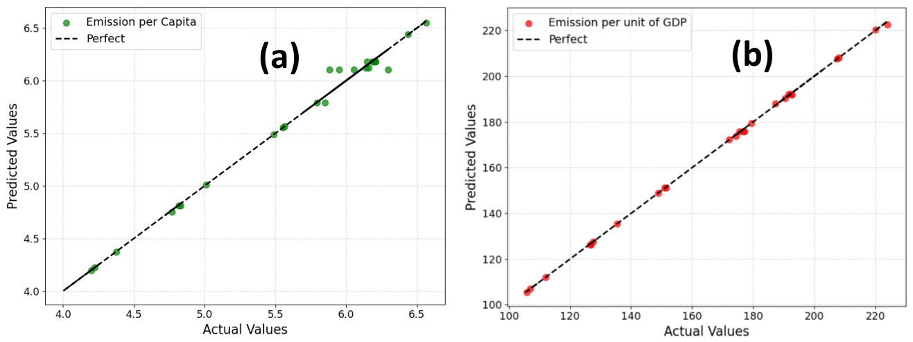
Figure 2 displays the predicted values as a function of the actual values. The points cluster closely around the ideal prediction line, demonstrating the strong agreement between the predicted and actual values. This figure visually confirms the model's accuracy, particularly when CO2 emissions per unit of GDP exhibit near-perfect linearity (Figure 3-b), compared to emissions per capita (Figure 3-a).
Figure 2.
Linearity of predicted values against actual values of CO2 emissions per capita (a) and per unit of GDP (b) using DT model.
Figure 2.
Linearity of predicted values against actual values of CO2 emissions per capita (a) and per unit of GDP (b) using DT model.
3.2. Modeling Study by Ann Model
Using the ANN model involves several important steps [22]. First, we begin with a data overview, which consists of defining eight input variables and creating visual aids for key target variables, such as CO2 emission estimates. Next, the networks are trained and tested. Specifically, we normalize the data using the Standard Scaler method. Once normalized, the data is divided into two sets, one for training and the other for testing. The ANN has a single hidden layer composed of 300 neurons and uses the logistic function as its activation function.
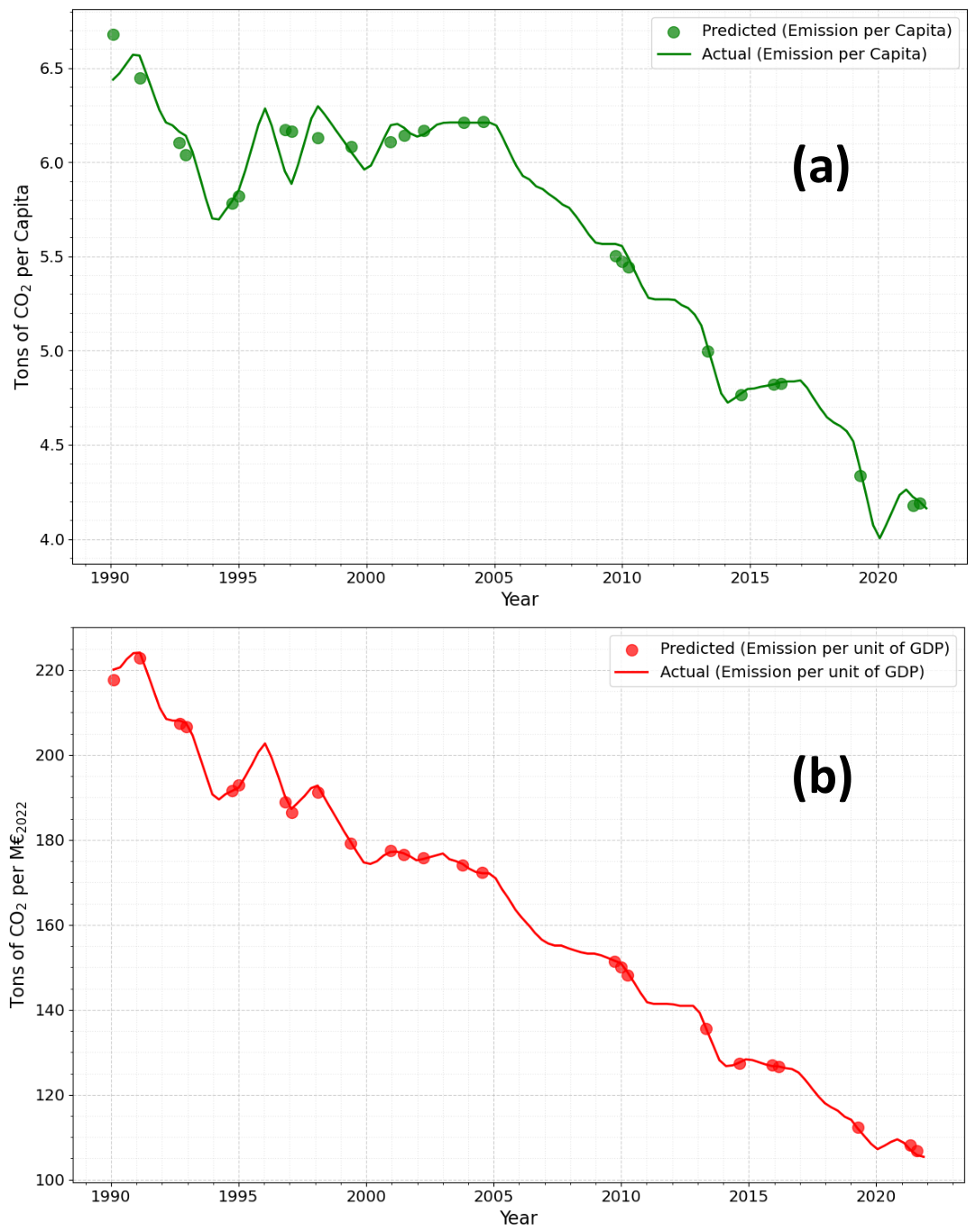
Once the optimal model is established, we evaluate its effectiveness using metrics essential to our analysis, which provide measurable information about the accuracy of the model's predictions. In Figure 3, we presented the evolution of the predicted and actual CO2 emissions per capita and per unit of GDP using ANN model
Figure 3.
Predicted and actual CO2 emissions per capita (a) and per unit of GDP (b) using ANN model.
Figure 3.
Predicted and actual CO2 emissions per capita (a) and per unit of GDP (b) using ANN model.
The different values of the evaluation parameters are given in Table 2.
With values of 0.01, 0.068, and 0.1 for MAE, MSE, and RMSE, respectively, the ANN model shows high predictive efficiency, indicating small discrepancies between predicted and actual values in CO₂ emissions modeling. Furthermore, the coefficient of determination (R²) is very close to unity, highlighting the model's excellent predictive performance for estimating CO2 emissions per unit of GDP.
Figure 4 shows a comparison between the CO2 emission estimates obtained by the ANN model and the actual data values. Unlike the variation of the emission values per unit of GDP, the predicted curves for CO2 emissions per capita do not closely match the actual curves.
3.3. Mathematical Model Using Interpolation Algorithm
In the mathematical model, two interpolation methods were used to estimate missing or future values from our real data. The first method, called Interpolator 1, uses linear interpolation, which constructs straight line segments between consecutive known data points. This approach is simple, computationally efficient, and suitable for data with nearly constant rates of change. However, it can produce less smooth curves. The second method, called Interpolator 2, applies cubic interpolation, which fits smooth cubic polynomials between data points to generate a more natural and continuous curve. This technique is particularly advantageous when the data varies continuously, although it is more computationally intensive and can become less reliable at the boundaries when the data is sparse or noisy. Interpolator 2 model was adopted in the remainder of this study as it showed a modeling closer to the real variations than Interpolator 1.
Figure 5 presents the modeling of our data using a mathematical model. This graph shows a good agreement between the model used and the real data, whether for CO2 emissions per capita or per unit of GDP.
As presented in Table 3, the interpolation model demonstrated good predictive performance, with a MAE of 0.025, an MSE of 0.0016, and an RMSE of 0.04, indicating minimal discrepancies between predicted and actual per capita CO2 emissions. Furthermore, the coefficient of determination (R²) reached 0.999 for the CO2 emissions per unit of GDP model, highlighting the robustness and high accuracy of the proposed approach.
Figure 6 presents a comparison between the CO₂ emission estimates generated by the ANN model and the corresponding actual data.
For CO₂ emissions per capita, the points are generally aligned along the ideal line, indicating that the model accurately reproduces the overall trend. However, there is slightly more dispersion, especially for some intermediate values. This reflects moderate accuracy, with small prediction errors. Regarding CO₂ emissions per unit of GDP, the points are very close to the ideal line, showing excellent agreement between predicted and actual values. Dispersion is minimal, indicating very high accuracy of the ANN model for this indicator. This behavior is consistent with the metrics error values given in Table 3.
3.4. Comparison Between Models and Co₂ Emissions Forecasts
The models were tested on two targets; emissions per capita and emissions per unit of GDP. By comparing the different results, we observe that the DT and ANN models exhibit the lowest RMSE values for per capita CO2 emissions, demonstrating their high predictive accuracy. In contrast, the ANN models for GDP show higher RMSE values, indicating a greater deviation from actual values. The remarkably low RMSE value of the DT model (0.006) underscores its exceptional effectiveness in predicting per capita CO₂ emissions. The mathematical model based on interpolation achieves the lowest MAE value, with a very low error of 0.025 for CO2 emissions per capita. The DT model achieves an R² value of 0.999, which suggests that the model takes into account almost all differences in the data and provides a near-perfect prediction of CO2 emissions for each unit of GDP. For CO2 emissions per capita, the interpolation model achieves the lowest MAE (0.025) with a very high R² of 0.996, indicating excellent fit and superior accuracy for this data category. For emissions per unit of GDP, both DT and ANN achieved a perfect coefficient of determination (R²) of 0.999. However, the ANN exhibited a slightly lower MAE value (0.64 vs. 0.379 for the decision tree) but a significantly higher MSE. Interpolation is less effective in this category, with larger errors. Therefore, the decision tree is the most balanced and reliable overall model, particularly for emissions per unit of GDP, given its accuracy and stability for both targets.
For these reasons, we have adopted the DT and Interpolation models to make CO2 emission forecasts up to the year 2030. In Figure 7, we presented the evolution of forecasts CO2 emissions per capita by mathematical model and per unit of GDP using DT model.
The different parameters for evaluating this forecasting are given in Table 4. The mathematical model achieves a very low MAE of 0.0258 and RMSE of 0.0408, along with a high R² of 0.9967. These metrics confirm the model's high precision in forecasting emissions per capita with strong reliability. The visual trend in Figure 7 reflects a near-perfect prediction fit, aligning smoothly with historical data. Values in table 4 validates this with an extremely high R² of 0.9998 and acceptable error margins (MAE = 0.3795, RMSE = 0.5606), showing high predictive power. The DT model effectively captures the economic-environmental relationship.
The values of the various evaluation criteria, which are specific to these models, indicate considerable reliability of these predictions. According to these forecasts, per capita CO₂ emissions continue their downward trend, while emissions per unit of GDP remain broadly stable through 2030. These results are of major importance from both an environmental and economic perspective. Indeed, the combined analysis of these trends can guide the development of appropriate economic strategies, enabling the anticipation and implementation of preventative measures aimed at further reducing CO2 emissions. Future work may focus on integrating additional variables, exploring hybrid models, and improving real-time prediction capabilities to further enhance forecasting accuracy and applicability.
4. Conclusions
This study presented a comprehensive comparative analysis of machine learning approaches, including Artificial Neural Networks (ANN), Decision Trees (DT), and interpolation methods, for predicting CO2 emissions per capita and per unit of GDP in France. The results demonstrate that all models achieve high predictive performance, with notable differences depending on the target variable. The results show that the interpolation model excels in predicting CO2 emissions per capita, with minimal error and a near-perfect fit. For emissions relative to GDP, the decision tree model stands out for its excellent balance between accuracy and consistency, outperforming both ANN and interpolation. While ANN models offer competitive results, their higher margins of error make them less robust in both cases. The forecasting analysis up to 2030 reveals a continued decline in per capita CO2 emissions, while emissions relative to GDP remain relatively stable. These trends suggest a potential decoupling between economic growth and environmental impact, which is a key objective in sustainable development strategies. The findings confirm the relevance and efficiency of machine learning techniques as powerful tools for environmental monitoring and policy support. The proposed framework can assist decision-makers in designing targeted mitigation strategies and can be extended to other contexts, provided that reliable datasets are available. The findings confirm the superiority of machine learning models over traditional statistical methods, offering reliable tools for forecasting climate impacts.
Author Contributions
Conceptualization, R.L. and M.R.; investigation, R.L. and W.H.; methodology, R.L.; validation, A.M.; formal analysis, A.M. and W.H.; data curation, W.H. and K.L.; writing—original draft preparation, R.L. and K.L.; writing—review and editing, A.M. and M.R.; supervision, M.R. All authors have read and agreed to the published version of the manuscript.
Funding
Not applicable.
Informed Consent Statement
Informed consent: Not applicable.
Data Availability Statement
No datasets were generated or analyzed during the current study.
Ethics Approval and Consent to Participate
Not applicable.
Acknowledgments
The authors would like to express their sincere gratitude to all the managers and members of the Laboratory of Metrology and Energy Systems and the Laboratory of Nanomaterials, Nanotechnology and Energy for their valuable scientific support and assistance.
Conflicts of Interest
Disclosure statement: The authors have no relevant financial and nonfinancial interests to disclose.
References
- Hamrouni, D.; Hasni, R.; Ben Jebli, M. The Impact of Economic Complexity in Trade, Technology, and Research on CO2 Emissions: Evidence from OECD Countries. Environ. Model. Assess. 2025, 30, 487–504. [CrossRef]
- Şahin, S. Digital-economic transformation’s environmental impact: transportation CO2 emissions in fragile and transition economies. Transp. Res. Part D: Transp. Environ. 2025, 150. [CrossRef]
- Ghoshray, A.; Lorusso, M. Energy consumption, CO2 emissions and economic growth in selected ASEAN countries. Lett. Spat. Resour. Sci. 2025, 18, 1–14. [CrossRef]
- Filonchyk, M.; Peterson, M.P.; Zhang, L.; Hurynovich, V.; He, Y. Greenhouse gases emissions and global climate change: Examining the influence of CO2, CH4, and N2O. Sci. Total. Environ. 2024, 935, 173359. [CrossRef]
- Ajala, A.A.; Adeoye, O.L.; Salami, O.M.; Jimoh, A.Y. An examination of daily CO2 emissions prediction through a comparative analysis of machine learning, deep learning, and statistical models. Environ. Sci. Pollut. Res. 2025, 32, 2510–2535. [CrossRef]
- Jin, Y.; Sharifi, A.; Li, Z.; Chen, S.; Zeng, S.; Zhao, S. Carbon emission prediction models: A review. Sci. Total. Environ. 2024, 927, 172319. [CrossRef]
- Tian, Y.; Ren, X.; Li, K.; Li, X. Carbon Dioxide Emission Forecast: A Review of Existing Models and Future Challenges. Sustainability 2025, 17, 1471. [CrossRef]
- Meng, Y.; Noman, H. Predicting CO2 Emission Footprint Using AI through Machine Learning. Atmosphere 2022, 13, 1871. [CrossRef]
- Khemissi, I.; Laajimi, R.; Ben Mabrouk, K.; Hajjaji, A.; Rahmani, M. An in-depth study by machine learning models of the absorbance properties of stable Ta2O5 nanotubes decorated by PbS nanoparticles for photocatalytic applications. Mater. Res. Bull. 2024, 184. [CrossRef]
- Laajimi, K.; Elhadjamor, E.A.; Laajimi, R.; Rahmani, M.; Gazzah, M.H. Modeling study of the magnetocaloric behavior of La₀.₆₇Ca₀.₃₃Mn₀.₉₈Ni₀.₀₂O₃ alloys using artificial neural networks. Results Eng. 2025, 26. [CrossRef]
- Copeland, B.J. The Turing test. Minds Mach. 2000, 10, 519–539.
- Ollis, D. Kinetics of photocatalytic, self-cleaning surfaces: A decision tree approach for determination of reaction order. Appl. Catal. B: Environ. 2019, 242, 431–440. [CrossRef]
- Javed, M.F.; Shahab, M.Z.; Asif, U.; Najeh, T.; Aslam, F.; Ali, M.; Khan, I. Evaluation of machine learning models for predicting TiO2 photocatalytic degradation of air contaminants. Sci. Rep. 2024, 14, 1–25. [CrossRef]
- Tudoroiu, S.-C.; Tudoroiu, R.-E. Modelling the Strategic Process Planning for a Medium Size Company in The German Photovoltaic Industry by Using Decision Trees. Procedia Comput. Sci. 2026, 278, 2019–2027. [CrossRef]
- Barakat, S.; Elkhouly, H.I.; Sofey, A.; Harraz, N. A hybrid machine learning model for predicting agricultural production costs: Integrating economic sensitivity analysis and environmental factors in Egypt. J. Environ. Manag. 2025, 390, 126371. [CrossRef]
- Yang, G.R.; Wang, X.-J. Artificial Neural Networks for Neuroscientists: A Primer. Neuron 2020, 107, 1048–1070. [CrossRef]
- Laajimi, R.; Laajimi, K.; Rahmani, M. Deep characterization of the electrical features of Ag/P3HT/SiNWs Schottky diodes by machine learning models based on experimental study. Surfaces Interfaces 2024, 54. [CrossRef]
- Honda, H.; Yamamoto, M.; Arata, S.; Kobayashi, H.; Inagaki, M. Decision tree–based identification of Staphylococcus aureus via infrared spectral analysis of ambient gas. Anal. Bioanal. Chem. 2021, 414, 1049–1059. [CrossRef]
- Miao, L.; Gao, M.; Xiao, W.; Kang, Y.; Li, R.; Kong, H.; Mou, H.; Chen, W.; Ao, T. Progress toward adsorption mechanism exploration method for capacitive deionization: Experimental, mathematical model, computational chemistry and machine learning. Desalination 2024, 586. [CrossRef]
- Rainio, O.; Teuho, J.; Klén, R. Evaluation metrics and statistical tests for machine learning. Sci. Rep. 2024, 14, 1–14. [CrossRef]
- Maiorino, A.; Del Duca, M.G.; Tomc, U.; Tušek, J.; Kitanovski, A.; Aprea, C. A numerical modelling of a multi-layer LaFeCoSi Active magnetic regenerator by using Artificial Neural Networks. Appl. Therm. Eng. 2021, 197. [CrossRef]
- Ramalingam, K.; Kandasamy, A.; Balasubramanian, D.; Palani, M.; Subramanian, T.; Varuvel, E.G.; Viswanathan, K. Forcasting of an ANN model for predicting behaviour of diesel engine energised by a combination of two low viscous biofuels. Environ. Sci. Pollut. Res. 2019, 27, 24702–24722. [CrossRef]
Figure 1.
Predicted and actual CO2 emissions per capita (a) and per unit of GDP (b) using DT model.
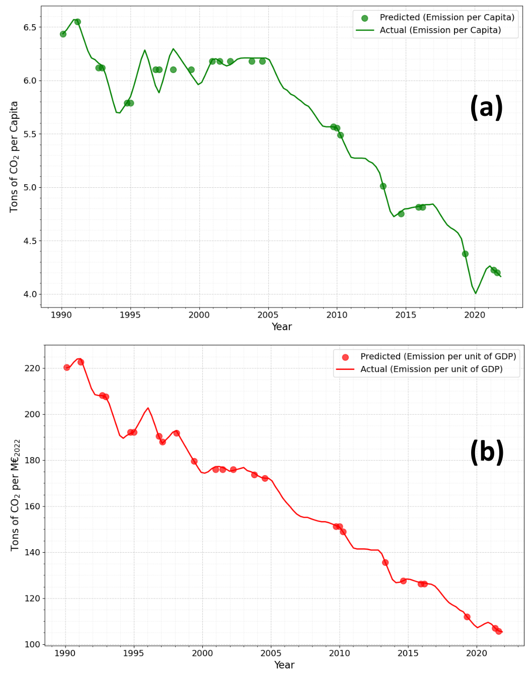
Figure 4.
Linearity of predicted values against actual values of CO2 emissions per capita (a) and per unit of GDP (b) using ANN model.
Figure 4.
Linearity of predicted values against actual values of CO2 emissions per capita (a) and per unit of GDP (b) using ANN model.
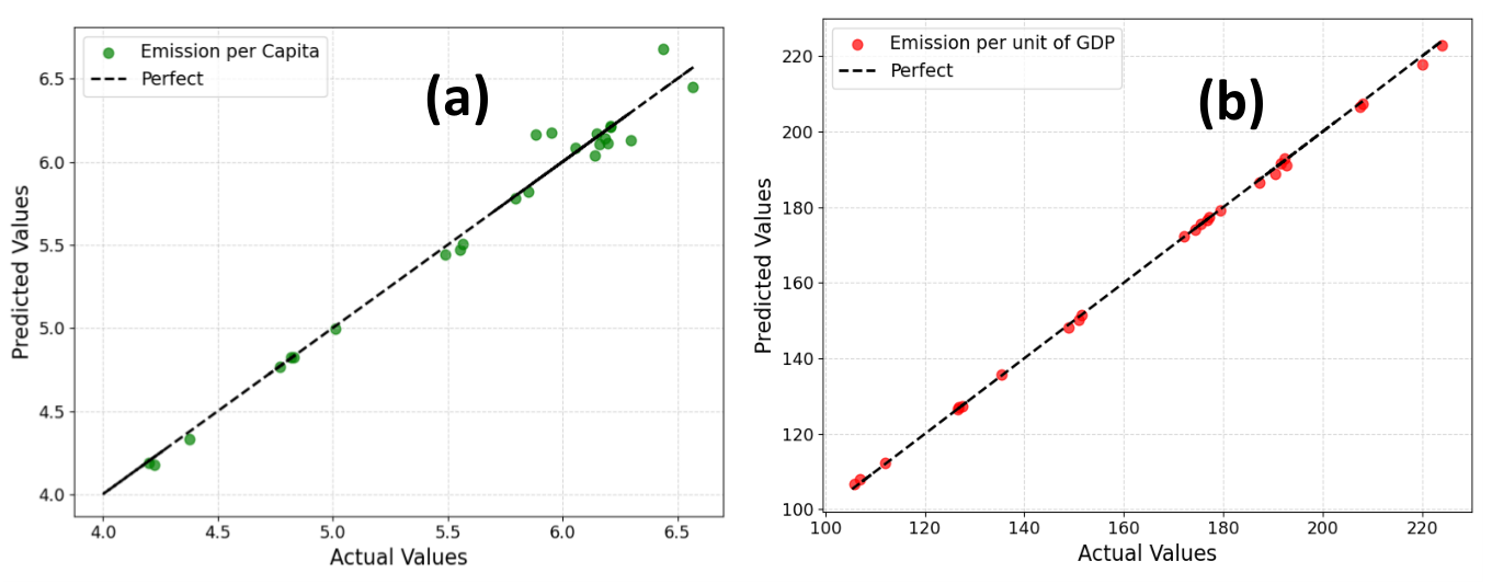
Figure 5.
Predicted and actual CO2 emissions per capita (a) and per unit of GDP (b) using interpolation model.
Figure 5.
Predicted and actual CO2 emissions per capita (a) and per unit of GDP (b) using interpolation model.
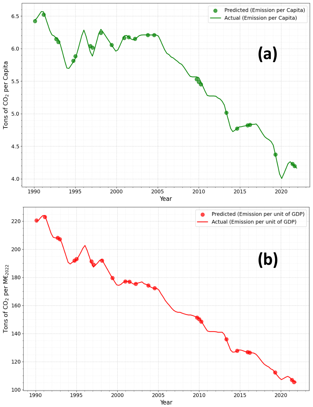
Figure 6.
Linearity of predicted values against actual values of CO2 emissions per capita (a) and per unit of GDP (b) using interpolation model.
Figure 6.
Linearity of predicted values against actual values of CO2 emissions per capita (a) and per unit of GDP (b) using interpolation model.
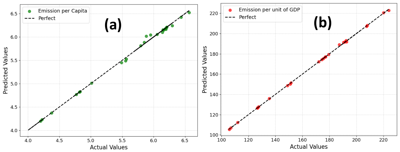
Figure 7.
Forecasts CO2 emissions per capita by mathematical model (a) and per unit of GDP using DT model (b).
Figure 7.
Forecasts CO2 emissions per capita by mathematical model (a) and per unit of GDP using DT model (b).
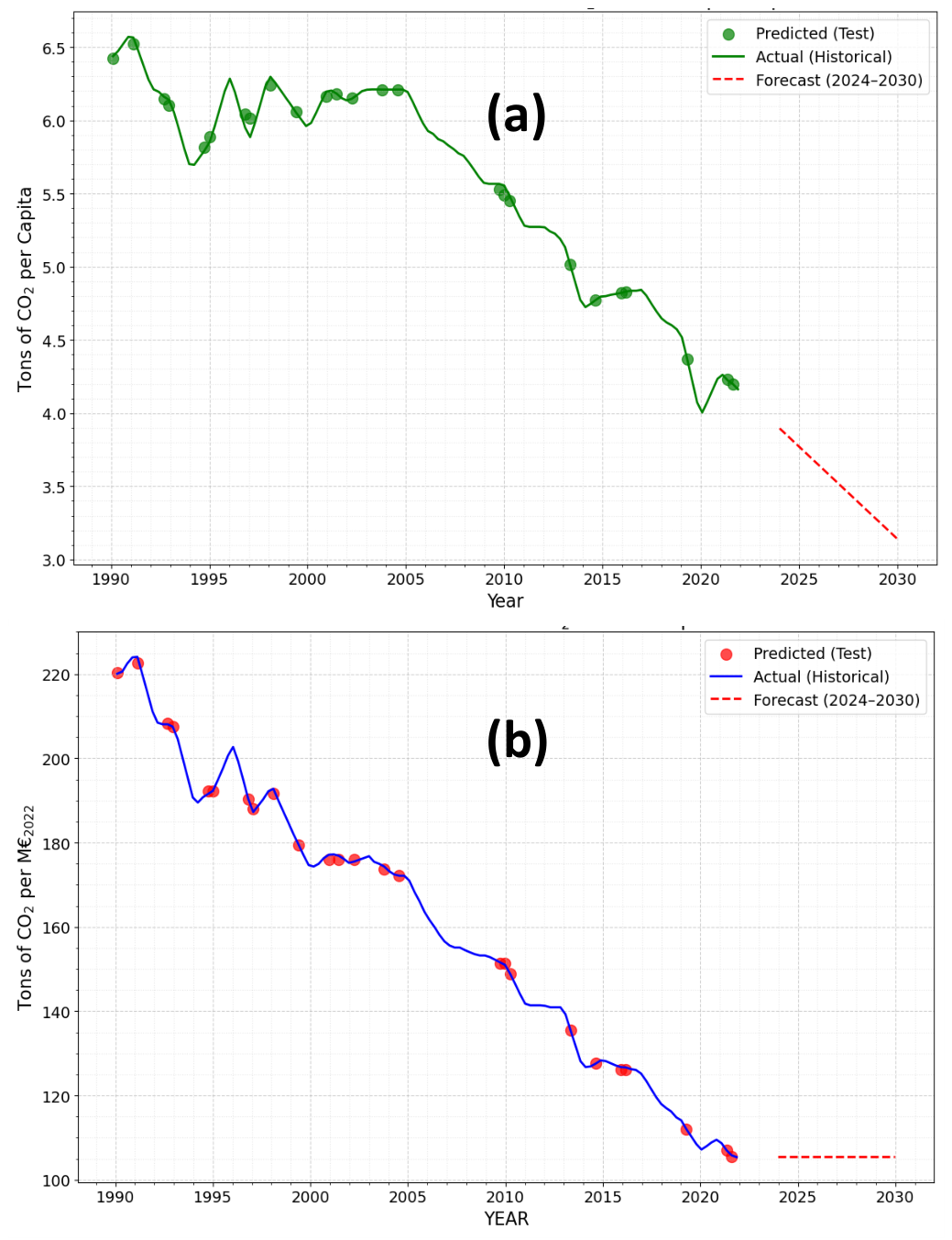
Table 2.
Evaluation results of ANN modeling of CO2 Emission.
| Evaluation criteria | MAE | MSE | RMSE | R2 |
| Emission per capita | 0.068 | 0.01 | 0.1 | 0.978 |
| Emission per unit of GDP | 0.64 | 0.73 | 0.85 | 0.999 |
Table 3.
Evaluation results of interpolation modeling of CO2 Emission.
| Evaluation criteria | MAE | MSE | RMSE | R2 |
| Emission per capita | 0.025 | 0.0016 | 0.04 | 0.996 |
| Emission per unit of GDP | 0.419 | 0.373 | 0.611 | 0.999 |
Table 4.
Evaluation results of forecasting CO2 emission.
| Evaluation criteria | MAE | MSE | RMSE | R2 |
| Emission per capita | 0.0258 | 0.0017 | 0.0408 | 0.9967 |
| Emission per unit of GDP | 0.3795 | 0.3143 | 0.5606 | 0.9998 |
Disclaimer/Publisher’s Note: The statements, opinions and data contained in all publications are solely those of the individual author(s) and contributor(s) and not of MDPI and/or the editor(s). MDPI and/or the editor(s) disclaim responsibility for any injury to people or property resulting from any ideas, methods, instructions or products referred to in the content. |
© 2026 by the authors. Licensee MDPI, Basel, Switzerland. This article is an open access article distributed under the terms and conditions of the Creative Commons Attribution (CC BY) license.
Copyright: This open access article is published under a Creative Commons CC BY 4.0 license, which permit the free download, distribution, and reuse, provided that the author and preprint are cited in any reuse.


