Submitted:
28 May 2026
Posted:
29 May 2026
You are already at the latest version
Abstract
This paper presents a simplified dimensionless model for predicting the electrical performance of photovoltaic (PV) modules under varying irradiance and temperature conditions. Unlike conventional equivalent-circuit models that require detailed parameter extraction, the proposed approach employs dimensional analysis to establish direct relationships between key PVoperating points and normalized environmental variables, without assuming a predefined physical model. The model is validated using experimental datasets from Sandia National Laboratories, covering a wide range of irradiance (100–1100 W/m²) and module temperatures (15°C–75°C). Model accuracy is evaluated using normalized root mean square error (nRMSE). The results demonstrate strong predictive capability, with average nRMSE values below 2.5% for maximum power point voltage and current, below 1% for maximum power, and low errors for open-circuit voltage and short-circuit current. The proposed model provides a computationally efficient and accurate alternative to conventional PV models. Moreover, the dimensionless framework offers strong potential for predicting the performance of complex multiphysics energy systems, where conventional equivalent-circuit-based approaches are often difficult to apply or fail to achieve satisfactory accuracy.
Keywords:
photovoltaic modeling
; dimensional analysis
; PV module performance
; photovoltaic performance prediction
; multiphysics systems modeling
1. Introduction
Accurate modeling of photovoltaic (PV) modules is essential for the analysis, design, control, and optimization of solar energy systems. Reliable PV models enable the prediction of electrical performance under varying environmental and operating conditions and are therefore widely used in system simulation, performance assessment, and energy management applications.
Existing PV modeling approaches can generally be classified into three categories. The first category includes equivalent-circuit models, such as the single-diode and double-diode models, which represent the PV device using electrical circuit elements and require parameter extraction procedures to determine the model parameters. Among these approaches, the single-diode model remains one of the most widely adopted methods due to its relatively simple structure and reasonable accuracy. Several studies have focused on improving parameter estimation techniques for diode-based models using manufacturer datasheet information and characteristic points of the I–V curve [1,2,3].
The second category consists of empirical and data-driven approaches, including the Sandia PV Array Performance Model [4], which relies on measured I–V characteristics and experimentally derived correlations to estimate module performance under varying operating conditions. The third category includes physics-based models derived from semiconductor transport equations, such as the Poisson and drift–diffusion equations, which provide detailed physical representation of PV devices but require extensive device information and significant computational resources [5].
Despite their widespread use, diode-equivalent circuit models present several limitations. First, the parameters of these models are generally not available in manufacturer datasheets and must be determined using nonlinear parameter extraction techniques, which often involve iterative numerical procedures and may suffer from convergence and initialization difficulties [6]. Second, many analytical formulations rely on simplifying assumptions that may not remain valid under all operating conditions. A review by [7] showed that several commonly used assumptions in single-diode formulations may produce non-physical parameter values under varying irradiance and temperature conditions. Third, the extracted parameters are typically determined under standard test conditions (STC) and must be adjusted for different environmental conditions using additional empirical relationships [8]. Furthermore, equivalent-circuit models inherently depend on predefined electrical circuit representations that only approximate the complex semiconductor processes governing PV module behavior [2,9,10].
These limitations motivate the development of alternative PV modeling approaches that reduce dependence on predefined circuit structures and iterative parameter extraction procedures. Dimensional analysis provides a systematic framework for establishing relationships between physical variables based on their fundamental dimensions, enabling predictive modeling without requiring detailed representation of the internal physical mechanisms of the system. Previous work by [11] demonstrated the applicability of dimensional analysis for estimating PV module efficiency; however, the approach was limited to efficiency prediction and did not address the direct prediction of PV electrical characteristics.
In this work, a dimensional analysis-based framework is proposed for predicting the electrical characteristics of photovoltaic modules under varying irradiance and temperature conditions. The proposed model predicts the short-circuit current (), open-circuit voltage (), and the current and voltage at the maximum power point ( and ) using relationships derived from normalized environmental and electrical variables. Unlike conventional diode-equivalent approaches, the proposed method does not rely on predefined circuit structures or iterative parameter extraction procedures. The model is validated using publicly available datasets from the Sandia National Laboratories PV Performance Modeling Collaborative database, which is widely used for benchmarking photovoltaic performance models.
2. Materials and Methods
2.1. Dimensional Analysis Framework
The current–voltage (I–V) characteristics of photovoltaic modules under varying irradiance and temperature conditions exhibit self-similar behavior, indicating the presence of scalable relationships between the governing variables. In such systems, dimensional analysis becomes a powerful tool for identifying the underlying mathematical relationships among the variables describing the system [12]. Consequently, dimensional analysis can be applied to derive a mathematical model describing the electrical behavior of photovoltaic modules. Dimensional analysis provides a systematic framework for establishing relationships between physical variables based on their fundamental dimensions and is commonly implemented using the Buckingham theorem [13]. A detailed description of the dimensional analysis methodology applied to photovoltaic systems was presented in [11]. Therefore, only the steps relevant to the development of the present model are summarized in the next subsection.
2.2. Selected Variables
The PV module is modeled using irradiance G and temperature T as inputs, and electrical parameters , , , and as outputs. These variables form the basis for deriving dimensionless relationships.
2.3. Dimensionless Relationships
In previous work [11] dimensional analysis was applied to derive a relationship describing the efficiency of photovoltaic modules as a function of normalized environmental variables. The PV module efficiency was expressed as:
where:
and are the normalized irradiance and temperature variables, respectively. and are the model cofficents for the temperature and irradiance.
denote the efficiency, irradiance and module temperature under standard test conditions.
Equation (1) represents the first equation in the proposed model.
In this work, the ratio between the open-circuit voltage and the short-circuit current is defined as
The new dimensionless parameter was found to follow a power-law trend that remains approximately consistent across different PV modules. Based on this observation, the ratio between voltage and current can be expressed as
where a and b are the second set of model coefficients determined during the model development process. The second dimentionless equation of the proposed model describes the relationship between the normalized parameter and the normalized environmental variables. Based on the dimensional analysis framework, this relationship can be expressed as
where and , are the model coefficients for the temperature and irradiance variables, respectively.
In order to extend the proposed model to predict the open-circuit voltage and short-circuit current, an additional dimensionless Paramter F is introduced. Similar to the previous formulations, a relationship links the normalized parameter to the normalized environmental variables as follows:
where , and , are the model coefficients for the temperature and irradiance variables, respectively.
are the model coefficients that represent the effect of temperature on the PV module performance, while represent the irradiance coefficients. The dimentionless relationships are sumerized in Figure 1, which shows the structure of the proposed model and the sequence used to derive the electrical parameters of the photovoltaic module.
2.4. PV Parameter Expressions
Using the derived relationships, the electrical parameters are obtained as functions of and :
2.5. Data Extraction
The I–V curves of the selected photovoltaic module (GCL-M10/72H) were digitized from the manufacturer datasheet using WebPlotDigitizer [14]. Key electrical parameters, including the short-circuit current (), open-circuit voltage (), and maximum power point (), were extracted under different irradiance and temperature conditions, as illustrated in Figure 2.
The values of , , , and obtained from the digitized I–V curves under different environmental conditions are presented in Table 2. Using the extracted electrical parameters and equations from 1 to 9 from the previous section the corresponding normalized parameters , , and were then determined. The calculated results are also summarized in Table 1.
2.6. Coefficient Determination
Model coefficients were obtained by fitting the dimensionless relationships to the extracted dataset. The results are summarized in Table 2.
3. Model Validation
3.1. Validation Dataset
The proposed model was validated using experimental photovoltaic module datasets obtained from Sandia National Laboratories through the PV Performance Modeling Collaborative database [15] Simplified method for predicting photovoltaic array output. These datsets contain detailed electrical measurements of photovoltaic modules obtained under controlled laboratory conditions and are widely used for benchmarking photovoltaic performance models. The experimental measurements were conducted according to the procedures specified in IEC 61853-1, which defines a matrix of irradiance and temperature operating conditions for PV modules. The datasets include current–voltage (I–V) characteristics measured across irradiance levels typically ranging from 100 W/m² to 1100 W/m², and module temperatures varying approximately from 15°C to 75°C. For each module, the dataset includes 23 standardized operating points defined by the IEC 61853-1 test matrix, in addition to 17 supplementary measurement points provided at intermediate temperature conditions. In the present study, nine operating points were selected for extracting the coefficients of the proposed model. These points correspond to operating conditions that are commonly available in manufacturer datasheet I–V curves, which represent the most accessible source of information for photovoltaic module modeling. The remaining 31 operating points were used exclusively for model validation to assess the predictive capability of the developed model over a wide range of irradiance and temperature conditions. The operating conditions used for model coefficient extraction and validation are summarized in Table 3. The extraction set includes operating points corresponding to typical manufacturer datasheet conditions, while the validation set covers a wide range of irradiance and temperature values.
3.2. Extracted Model Coefficients
Using the procedure described in Section 2, the model coefficients were extracted for each PV module using the selected operating points. The resulting coefficients for the eight modules considered in this study are summarized in Table 4. The module efficiencies are also included to facilitate future comparisons between module performance and the obtained coefficients. These coefficients were subsequently used to predict the electrical characteristics of the PV modules under the remaining operating conditions for validation purposes. The small variation observed in the extracted coefficients across the eight modules suggests that the proposed dimensional-analysis formulation captures the key relationships governing PV module behavior. This indicates that the model may be applied to different module technologies with limited parameter variability.
The irradiance coefficients showed notably smaller deviations than the temperature coefficients , indicating that material response is more sensitive to temperature variations than to irradiance. This aligns with early PV models such as [16] , which disregarded irradiance effects. Additionally, excluding the HIT module would result in a lower standard deviation. Despite this variation, the overall dispersion of the coefficients remains limited across the analyzed modules.
3.3. Global Model Formulation
Based on the average values of the extracted coefficients reported in Table 4, the model equations can also be expressed in a global form using these mean coefficients. Substituting these mean coefficients into the model formulation yields the following simplified expressions:
These global expressions provide a simplified representation of the proposed model and may be useful for applications where module-specific calibration data are not available.
3.4. Applicability to Commercial PV Modules
To further evaluate the applicability of the proposed model using commonly available manufacturer information, the model coefficients were also extracted for eight additional commercial PV modules using datasheet electrical characteristics. The resulting coefficients are summarized in Table 5
The average coefficients derived from the commercial module datasheets show good agreement with those obtained from the Sandia laboratory datasets. This consistency suggests that the proposed model coefficients can be reliably determined using commonly available manufacturer datasheet information.
4. Results
The prediction accuracy of the proposed model was evaluated using the normalized root mean square error (nRMSE) calculated for the 31 validation operating points described in Table 3. The normalized root mean square error (nRMSE), which quantifies the deviation between predicted and measured values over the validation dataset defined as
Where:
= predicted value from the model
= measured value
N= number of validation points (31)
= average of the measured values
The nRMSE values were calculated for for each of the analyzed PV modules. The nRMSE values were computed for the predicted electrical parameters of each PV module using the 31 validation operating points spanning different irradiance and temperature conditions. The evaluation includes the parameters . The resulting nRMSE values for the eight PV modules are presented in Table 6.
The prediction accuracy of the proposed model for the electrical parameters of the analyzed PV modules is summarized in Table 7 in terms of the normalized root mean square error (nRMSE). The results show very good agreement between the predicted and measured values for all modules and operating conditions considered in the validation dataset. These relatively low error values indicate that the proposed model is capable of accurately reproducing the electrical characteristics of PV modules over a wide range of irradiance and temperature conditions. Furthermore, consistent prediction accuracy is observed across modules based on different technologies, including monocrystalline, polycrystalline, and heterojunction (HIT) modules, confirming the robustness of the proposed dimensional-analysis formulation.
Figure 3 shows the comparison between measured and modeled values for the electrical parameters, including , , , and . The results demonstrate a strong agreement, with most data points closely distributed around the ideal agreement line. The proposed model demonstrates good agreement with the experimental data across a wide range of operating conditions.
5. Discussion
Overall, the proposed dimensional-analysis-based model provides accurate predictions with low computational complexity, making it suitable for performance estimation and system-level simulations. The results show very good agreement between the predicted and measured values for all modules and operating conditions considered in the validation dataset. The average nRMSE values are 1.993% for , 2.260% for , 1.287% for , 0.454% for , and 0.880% for . These relatively low error values indicate that the proposed model is capable of accurately reproducing the electrical characteristics of PV modules over a wide range of irradiance and temperature conditions. In particular, the prediction error for the maximum power , which represents the most relevant parameter for PV system performance evaluation, remains below 1% on average. Furthermore, consistent prediction accuracy is observed across modules based on different technologies, including monocrystalline, polycrystalline, and heterojunction (HIT) modules, confirming the robustness of the proposed dimensional-analysis formulation.
6. Conclusions
This study presented a photovoltaic module modelling approach based on dimensional analysis for predicting the electrical characteristics of PV modules under varying environmental conditions. The model coefficients were extracted using a limited set of operating points corresponding to conditions typically available in manufacturer datasheet I–V curves. The proposed formulation was validated using experimental datasets from Sandia National Laboratories covering irradiance levels from 100 to 1100 W/m² and module temperatures ranging from approximately 15°C to 75°C. The validation results demonstrated good agreement between the predicted and measured electrical parameters. The results indicate that the proposed model is capable of accurately reproducing the electrical behavior of PV modules across a wide range of operating conditions. In particular, the low prediction error for the maximum power demonstrates the model’s suitability for PV performance evaluation and system-level simulations. Furthermore, the prediction errors were shown to be comparable to or lower than the measurement uncertainty associated with flash testing of PV modules, which further supports the reliability of the proposed formulation. The model also demonstrated consistent performance across modules based on different technologies, including monocrystalline, polycrystalline, and heterojunction modules, highlighting its robustness and general applicability. Beyond the specific application to photovoltaic modeling, this work also highlights the potential of dimensional analysis as an effective modeling framework for engineering systems. Although dimensional analysis has traditionally been applied mainly in fields such as fluid dynamics and heat transfer, its use in electrical and energy systems remains relatively limited. The results presented in this study demonstrate that dimensional analysis can provide a systematic and physically meaningful approach for modeling the behavior of photovoltaic devices using a reduced set of parameters and operating points. This capability suggests that the methodology may be extended to other complex and multiphysics engineering systems where interactions between electrical, thermal, and environmental variables are present. Consequently, the proposed approach may open new opportunities for applying dimensional analysis to a wider range of engineering problems, particularly in electrical engineering applications where such methods have been rarely explored. Future work may focus on validating the proposed model using outdoor experimental measurements and extending the analysis to additional photovoltaic technologies, including emerging devices such as perovskite-based modules. In addition, the dimensional-analysis framework presented in this study could be further explored for modeling other complex electrical and multiphysics engineering systems.
Author Contributions
Conceptualization, Samah Hashim. and Mohammed H. Siddig; methodology, Samah Hashim. and Mohammed H. Siddig; software, Samah Hashim; validation, Samah Hashim. and Mohammed H. Siddig.; formal analysis, Samah Hashim. and Mohammed H. Siddig; investigation, Samah Hashim. and Mohammed H. Siddig; resources, Samah Hashim. and Mohammed H. Siddig; data curation, Samah Hashim. and Mohammed H. Siddig; writing—original draft preparation, Mohammed H. Siddig; writing—review and editing, Samah Hashim. and Mohammed H. Siddig; visualization, Samah Hashim. ; supervision, Mohammed H. Siddig; project administration, Mohammed H. Siddig; All authors have read and agreed to the published version of the manuscript.
Funding
This research received no external funding.
Data Availability Statement
The datasets used in this study are publicly available from Sandia National Laboratories and were obtained from the Sandia Photovoltaic Performance Modeling Collaborative (PVPMC) database. Additional data extracted from manufacturer datasheets are available from the corresponding author upon reasonable request.https://pvpmc.sandia.gov. Other data will be available on request.
Conflicts of Interest
The authors declare no conflicts of interest.
Appendix A
Model Performance Under Different Operating Conditions
Figure A1.
Relative error of the predicted voltage at the maximum power point as a function of temperature for different irradiance levels for the analyzed PV modules.
Figure A1.
Relative error of the predicted voltage at the maximum power point as a function of temperature for different irradiance levels for the analyzed PV modules.

Figure A2.
Relative error of the predicted current at the maximum power point as a function of temperature for different irradiance levels for the analyzed PV modules.
Figure A2.
Relative error of the predicted current at the maximum power point as a function of temperature for different irradiance levels for the analyzed PV modules.

Figure A3.
Relative error of the predicted voltage and current at the maximum power point and as a function of temperature at constant irradiance for the analyzed PV modules.
Figure A3.
Relative error of the predicted voltage and current at the maximum power point and as a function of temperature at constant irradiance for the analyzed PV modules.

Appendix B Abbreviations
The following abbreviations are used in this manuscript:
| PV | Photovoltaic | |
| Photovoltaic module efficiency | ||
| Normalized module efficiency () | ||
| Module efficiency at standard test conditions | ||
| G | Solar irradiance | |
| Solar irradiance at standard test conditions | ||
| T | Module temperature | °C |
| Module temperature at standard test conditions | °C | |
| Normalized irradiance () | ||
| Normalized temperature () | ||
| Voltage at maximum power point | V | |
| Current at maximum power point | A | |
| Maximum power output of the PV module | W | |
| Open-circuit voltage | V | |
| Short-circuit current | A | |
| Ratio of open-circuit voltage to short-circuit current () | ||
| Normalized parameter () | ||
| F | Dimensionless parameter | |
| Normalized F parameter () | ||
| A | PV module area |
| Model coefficients in efficiency relation | ||
| Model coefficients in voltage–current relation | ||
| Model coefficients in normalized relation | ||
| Model coefficients in normalized F relation | ||
| STC | Standard Test Conditions | |
| RMSE | Root Mean Square Error | |
| nRMSE | Normalized Root Mean Square Error |
References
- Carrero, C.; Ramírez, D.; Rodríguez, J.; Platero, C.A. Accurate and fast convergence method for parameter estimation of PV generators based on three main points of the I–V curve. Renew. Energy 2011, 36, 2972–2977. [Google Scholar] [CrossRef]
- De Soto, W.; Klein, S.A.; Beckman, W.A. Improvement and validation of a model for photovoltaic array performance. Sol. Energy 2006, 80, 78–88. [Google Scholar] [CrossRef]
- Orioli, A.; Di Gangi, A. A procedure to calculate the five-parameter model of crystalline silicon photovoltaic modules on the basis of the tabular performance data. Appl. Energy 2013, 102, 1160–1177. [Google Scholar] [CrossRef]
- King, D.L.; Boyson, W.E.; Kratochvil, J.A. Photovoltaic Array Performance Model; Sandia National Laboratories: Albuquerque, NM, USA, 2004; pp. SAND2004–3535. [Google Scholar]
- van Roosbroeck, W. Theory of flow of electrons and holes in germanium and other semiconductors. Bell Syst. Tech. J. 1950, 29, 560–607. [Google Scholar] [CrossRef]
- Batzelis, E.I.; Papathanassiou, S.A. A method for the analytical extraction of the single-diode PV model parameters. IEEE Trans. Sustain. Energy 2016, 7, 504–512. [Google Scholar] [CrossRef]
- Khan, F.; Al-Ahmed, A.; Alsulaiman, F. Critical analysis of the limitations and validity of the assumptions with the analytical methods commonly used to determine the photovoltaic cell parameters: A review. Renew. Sustain. Energy Rev. 2021. [Google Scholar] [CrossRef]
- Anani, N.; Ibrahim, H. Adjusting the single-diode model parameters of a photovoltaic module with irradiance and temperature. Energies 2020, 13, 3226. [Google Scholar] [CrossRef]
- Duffie, J.A.; Beckman, W.A. Solar Engineering of Thermal Processes; Wiley: Hoboken, NJ, USA, 2013. [Google Scholar]
- Villalva, M.G.; Gazoli, J.R.; Filho, E.R. Comprehensive approach to modeling and simulation of photovoltaic arrays. IEEE Trans. Power Electron. 2009, 24, 1198–1208. [Google Scholar] [CrossRef]
- Siddig, M.H.; Hashim, S.M.; Osman, A.E. Formulation of an efficiency correlation for mono-crystalline PV modules using dimensional analysis. Sol. Energy 2020, 205, 456–460. [Google Scholar] [CrossRef]
- Barenblatt, G.I. Dimensional Analysis; Makinen, P., Translator; OPA: Amsterdam, The Netherlands, 1987. [Google Scholar]
- Buckingham, E. On physically similar systems; illustrations of the use of dimensional equations. Phys. Rev. 1914, 4, 345. [Google Scholar] [CrossRef]
- PlotDigitizer, version 3.1.6. Available online: https://plotdigitizer.com (accessed on 1 January 2026).
- PV Performance Modeling Collaborative (PVPMC). Available online: https://pvpmc.sandia.gov (accessed on 1 January 2023).
- Evans, D.L. Simplified method for predicting photovoltaic array output. Sol. Energy 1981, 27, 555–560. [Google Scholar] [CrossRef]
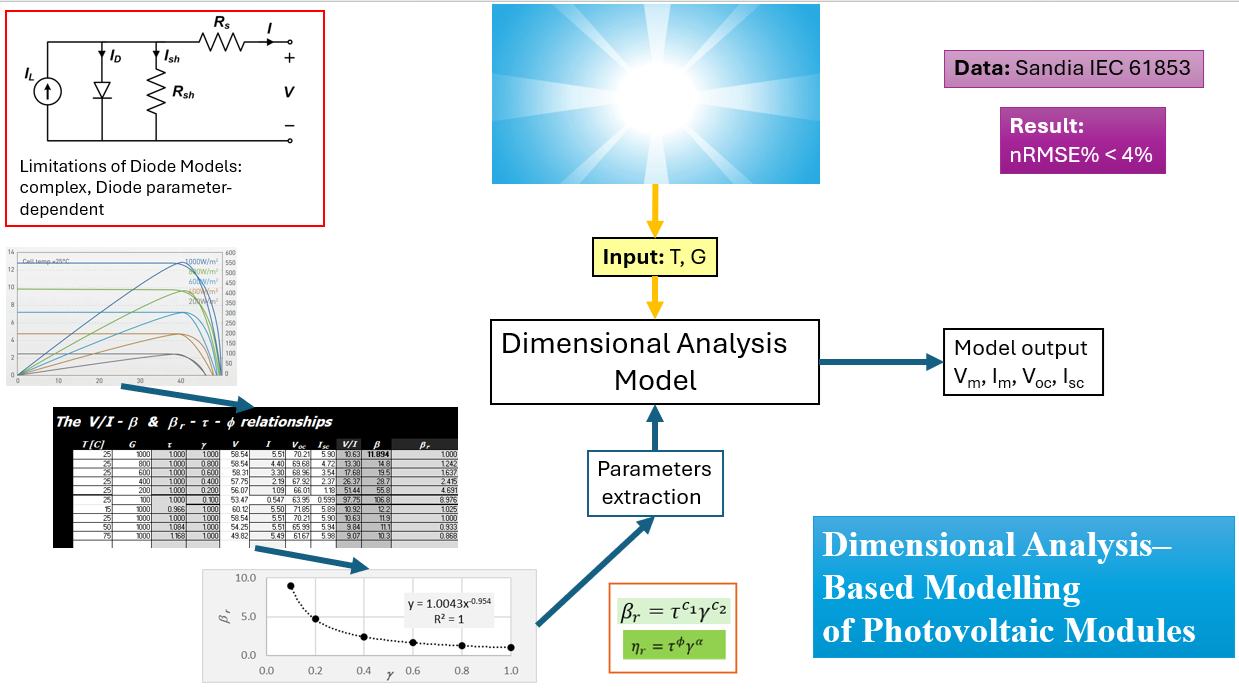
Figure 1.
Flow diagram of the proposed dimensional-analysis-based photovoltaic module model illustrating the relationships between environmental variables, normalized parameters, dimensionless model equations, intermediate electrical relations, and the resulting PV electrical characteristics.
Figure 1.
Flow diagram of the proposed dimensional-analysis-based photovoltaic module model illustrating the relationships between environmental variables, normalized parameters, dimensionless model equations, intermediate electrical relations, and the resulting PV electrical characteristics.

Figure 2.
Example of I–V curve digitization for the GCL-M10/72H module using WebPlotDigitizer [14], showing extracted data points and identification of key parameters (, , , and ).
Figure 2.
Example of I–V curve digitization for the GCL-M10/72H module using WebPlotDigitizer [14], showing extracted data points and identification of key parameters (, , , and ).

Figure 3.
Comparison between measured (by Sandia National Laboratories) and predicted (current model) PV electrical parameters (, , , and ) for 8 PV modules.
Figure 3.
Comparison between measured (by Sandia National Laboratories) and predicted (current model) PV electrical parameters (, , , and ) for 8 PV modules.


Table 1.
Electrical parameters extracted from the digitized I–V curves of the GCL-M10/72H photovoltaic module under different irradiance and temperature conditions, together with the calculated dimensionless quantities used for model coefficient determination
Table 1.
Electrical parameters extracted from the digitized I–V curves of the GCL-M10/72H photovoltaic module under different irradiance and temperature conditions, together with the calculated dimensionless quantities used for model coefficient determination
| Environmental Conditions | Normalized | Extracted Electrical Parameters | Calculated Quantities | |||||||
|---|---|---|---|---|---|---|---|---|---|---|
| T [°C] | G [W/m²] | Vmp [V] | Imp [A] | Voc [V] | Isc [A] | Fr | ||||
| 25 | 1000 | 1.000 | 1.000 | 41.992 | 13.223 | 50.391 | 13.911 | 1.000 | 1.001 | 1.000 |
| 25 | 800 | 1.000 | 0.800 | 41.690 | 10.667 | 49.105 | 11.134 | 1.217 | 1.002 | 0.975 |
| 25 | 600 | 1.000 | 0.600 | 41.614 | 8.000 | 49.029 | 8.330 | 1.625 | 1.000 | 0.971 |
| 25 | 400 | 1.000 | 0.400 | 41.690 | 5.251 | 48.348 | 5.553 | 2.403 | 0.986 | 0.958 |
| 25 | 200 | 1.000 | 0.200 | 41.992 | 2.557 | 47.213 | 2.749 | 4.741 | 0.967 | 0.926 |
| 10 | 1000 | 0.950 | 1.000 | 43.750 | 13.333 | 52.279 | 13.766 | 1.048 | 1.051 | 1.027 |
| 25 | 1000 | 1.000 | 1.000 | 41.618 | 13.333 | 50.147 | 13.889 | 0.997 | 1.000 | 0.994 |
| 40 | 1000 | 1.050 | 1.000 | 39.853 | 13.227 | 47.868 | 14.012 | 0.943 | 0.950 | 0.957 |
| 55 | 1000 | 1.101 | 1.000 | 37.279 | 13.280 | 45.515 | 14.134 | 0.889 | 0.892 | 0.918 |
| 70 | 1000 | 1.151 | 1.000 | 34.412 | 13.520 | 43.162 | 14.257 | 0.836 | 0.838 | 0.878 |
Table 2.
Model coefficients obtained for the GCL-M10/72H module
| a | b | ||||||
|---|---|---|---|---|---|---|---|
| -1.177 | 0.0226 | 0.8048 | 1.0594 | -1.180 | -0.971 | 0.816 | 0.0435 |
Table 3.
Operating conditions used for coefficient extraction and model validation
| Dataset Usage | Temperature (°C) | Irradiance (W/m²) | Description |
|---|---|---|---|
| Coefficient extraction (9) | 25 | 100, 200, 400, 600, 800, 1000 | Irradiance variation at 25°C |
| 15, 25, 50, 75 | 1000 | Temperature variation at 1000 W/m² | |
| Validation (31) | 15.3 – 74.76 | 1000 | Temperature sweep |
| 15 | 100 – 800 | Irradiance variation | |
| 50 | 100 – 1100 | ||
| 75 | 100 – 1100 |
Table 4.
Extracted Parameters for Different PV Module Technologies
| Module | Technology | a | b | Efficiency (%) | ||||||
|---|---|---|---|---|---|---|---|---|---|---|
| IT-360-SE72 | Mono | -1.339 | 0.027 | 0.823 | 1.027 | -1.068 | -0.955 | -0.844 | 0.047 | 0.178 |
| Q.PLUS-G4.1-280 | Poly | -1.442 | 0.032 | 0.840 | 1.020 | -1.153 | -0.955 | -0.934 | 0.044 | 0.166 |
| Q-Peak-G4-1-300 | Mono | -1.395 | 0.021 | 0.814 | 1.031 | -1.074 | -0.959 | -0.860 | 0.048 | 0.174 |
| VBHN325SA | HIT | -1.003 | 0.043 | 0.858 | 1.017 | -0.885 | -0.954 | -0.730 | 0.035 | 0.193 |
| LG320N1K | Mono | -1.386 | 0.021 | 0.838 | 1.020 | -1.069 | -0.961 | -0.892 | 0.021 | 0.187 |
| JKM260P | Poly | -1.467 | 0.048 | 0.828 | 1.028 | -1.176 | -0.956 | -0.942 | 0.057 | 0.158 |
| CS6K-275M | Mono | -1.442 | 0.020 | 0.803 | 1.047 | -1.153 | -0.958 | -0.934 | 0.051 | 0.169 |
| CS6K-270P | Poly | -1.421 | 0.044 | 0.907 | 1.000 | -1.162 | -0.957 | -0.921 | 0.053 | 0.163 |
| Average values | -1.362 | 0.032 | 0.839 | 1.024 | -1.093 | -0.957 | -0.882 | 0.044 | 0.173 | |
| Standard deviation | 0.133 | 0.010 | 0.028 | 0.012 | 0.084 | 0.002 | 0.063 | 0.010 | 0.010 | |
Table 5.
Model coefficients extracted from manufacturer datasheet parameters for eight commercial PV modules
Table 5.
Model coefficients extracted from manufacturer datasheet parameters for eight commercial PV modules
| Module | Technology | a | b | Efficiency% | ||||||
|---|---|---|---|---|---|---|---|---|---|---|
| CHSM60M-HC | (Mono) | |||||||||
| LR6-60PB | (Mono) | |||||||||
| BP 3220T | (Poly) | |||||||||
| GCL-M10/72H | (Mono) | |||||||||
| JAM60S01-300 | (Mono) | |||||||||
| HIT-240HDE4 | (HIT) | |||||||||
| SP 70 | (Mono) | |||||||||
| KD245GH-4FB2 | (Poly) | |||||||||
| Average values | ||||||||||
| Standard deviation |
Table 6.
Normalized root mean square error (nRMSE) values of the predicted electrical parameters for the eight PV modules using the 31 validation operating points.
Table 6.
Normalized root mean square error (nRMSE) values of the predicted electrical parameters for the eight PV modules using the 31 validation operating points.
| Module | Technology | nRMSE% | nRMSE% | nRMSE% | nRMSE% | nRMSE% |
|---|---|---|---|---|---|---|
| IT-360-SE72 | (Mono) | 2.1944 | 2.0553 | 1.0164 | 0.1899 | 0.7016 |
| Q.PLUS-G4.1-280 | (Poly) | 3.7735 | 2.1609 | 2.2968 | 2.2261 | 1.2969 |
| Q-Peak-G4-1-300 | (Mono) | 1.3611 | 2.0623 | 0.9926 | 0.1736 | 0.8951 |
| VBHN325SA | (HIT) | 2.3025 | 1.9908 | 0.7001 | 0.1548 | 0.7708 |
| LG320N1K | (Mono) | 1.6654 | 1.2051 | 2.0207 | 0.4737 | 0.8371 |
| JKM260P | (Poly) | 1.1222 | 1.8509 | 1.1273 | 0.1390 | 0.9221 |
| CS6K-275M | (Mono) | 1.1690 | 3.6558 | 1.1122 | 0.1509 | 0.7428 |
| CS6K-270P | (Poly) | 2.3559 | 3.0952 | 1.0321 | 0.1260 | 0.8757 |
| Average values | 1.993 | 2.260 | 1.287 | 0.454 | 0.880 |
Disclaimer/Publisher’s Note: The statements, opinions and data contained in all publications are solely those of the individual author(s) and contributor(s) and not of MDPI and/or the editor(s). MDPI and/or the editor(s) disclaim responsibility for any injury to people or property resulting from any ideas, methods, instructions or products referred to in the content. |
© 2026 by the authors. Licensee MDPI, Basel, Switzerland. This article is an open access article distributed under the terms and conditions of the Creative Commons Attribution (CC BY) license (http://creativecommons.org/licenses/by/4.0/).
Copyright: This open access article is published under a Creative Commons CC BY 4.0 license, which permit the free download, distribution, and reuse, provided that the author and preprint are cited in any reuse.


