

Submitted:
09 October 2026
Posted:
12 October 2026
Read the latest preprint version here
Abstract
Minimum Vertex Cover has a classical polynomial-time ratio of 2, and a manuscript released by the OpenAI Math Team in October 2026, not yet peer reviewed, reports a proof of the Unique Games Conjecture in the form that, by the theorem of Khot and Regev, makes every fixed ratio below 2 NP-hard. We present SALVADOR (v0.1.1), a worst-case O(n + m) ensemble of eleven candidate covers plus a swap-maximize refinement; it contains the Hvala ensemble, so it is valid and has ratio at most 2 on every graph. We analyse each strategy c1, . . . , c12 separately and prove what it guarantees: c4 is exact on forests, cycles and complete graphs, and c4 and c8 are exact on every bipartite graph whose components are regular or degree-separated, which includes all regular bipartite graphs of every degree; c8 meets the Caro–Wei bound on every graph; c1, c5 have ratio 2ν/τ; c2 has ratio 11/6 on subcubic graphs; c3 beats 2 on hub-dominated graphs; c10 solves a labelled, weighted edge-dominating-set gadget whose optimum is a minimum vertex cover with the fewest doubly covered edges, by a dynamic program whose bags never exceed six nodes; c11 is exact when its elimination core is empty; and c9, c12 never worsen the best cover. Combining these certificates, SALVADOR has ratio at most 1.999999999 on every graph outside a residue R of nearly K˝onig–Egerváry graphs. We then explain why the ensemble succeeds on R: every cover satisfies the exact identity |C| = |y| + y(E(C)) + defy(C) for every fractional matching y, so on R the excess of a cover is its violation of complementary slackness, and the a-posteriori certificate |C|/νf equals the true ratio up to a factor 1 + 5 · 10−10; the strategies keep this violation small, and on regular graphs it is exactly the number of doubly covered edges, the quantity that c10 minimises. Experimentally, on 1,744 benchmark graphs, 152 bipartite graphs, 117 Khot–Regev YES instances, 120 mechanism instances and 267 regular graphs of degree up to 64, every instance carries a per-instance certificate of ratio at most 1.237, the ratio never exceeds 1.0455 on bipartite graphs and 1.0425 on YES instances with known optimum, all 117 regular bipartite graphs are solved exactly, and the bags of c10 never exceed six nodes. If the reported hardness holds, a proof that SALVADOR achieves 2 − ε0 on all of R would imply P = NP; we state this as a conditional theorem, not as a result.
Keywords:
vertex cover
; approximation algorithm
; ensemble heuristics
; bipartite planar reduction
; local search
; unique games conjecture
; P versus NP
MSC: 05C69; 05C70; 68Q25; 90C27
1. Introduction
The Minimum Vertex Cover (VC) problem is one of the twenty-one NP-complete problems identified by Karp [1]. Given an undirected graph , a set is a vertex cover if every edge of E has at least one endpoint in C; the goal is to find a minimum-cardinality vertex cover, denoted . Vertex cover is central to computer science, modelling guard placement, network monitoring, error-correcting codes, and serving as the canonical starting point for parameterised and approximation algorithms.
The approximation landscape for VC is unusually well charted. The classical maximal-matching algorithm achieves a 2-approximation in linear time [2]; LP-based refinements by Karakostas [3] and Karpinski and Zelikovsky [4] reach factor , which is but falls short of a constant . From the hardness side, Dinur and Safra [5] ruled out any ratio below under . Under the Unique Games Conjecture [6], Khot and Regev [7] showed that no polynomial-time algorithm can approximate Minimum Vertex Cover within factor for any fixed unless , and Austrin, Khot and Safra [8] refined this to graphs of maximum degree d, where the UGC-hardness threshold is , matching the algorithm of Halperin [9]. In October 2026 the OpenAI Math Team released a manuscript, The Unique Games Theorem, with accompanying Lean artifacts [10], which reports a deterministic polynomial-time reduction from 3SAT to unique games with completeness and soundness , that is, a proof of UGC in the NP-hardness form that Khot–Regev requires. At the time of writing this manuscript has not been peer reviewed. If it holds, the theorem of Khot and Regev makes every fixed ratio below 2 NP-hard, and the factor 2 is the exact polynomial-time barrier for Vertex Cover: a proved constant ratio with for a polynomial-time algorithm on every graph would imply , however small is, and no intermediate threshold such as needs to be crossed.
Against this backdrop, we present an algorithm—implemented as the Salvador Python package (v0.1.1)—that produces a vertex cover whose size is provably never more than twice the optimum and, on every instance we have tested under the default call , far closer to it. The algorithm, called FindVertexCover, is an ensemble: it computes eleven valid candidate covers, refines each by a swap-maximize pass, and returns the smallest refined cover. Four of the candidates and the pruning pass adapt the ensemble published as the Hvala algorithm [11,12], which proves an unconditional time and space bound and worst-case approximation ratio at most 2; Salvador therefore contains Hvala. Salvador adds seven candidates of its own and the final refinement, described below. The algorithm operates in five phases.
- 1.
- Preprocessing. Self-loops are discarded; isolated vertices are removed (they appear in no edge and need not be covered).
- 2.
- Ensemble of linear-time candidates. Seven independent heuristics are run on the cleaned graph G: maximal matching, bucket-queue maximum-degree greedy, and a degree-1 weighted-reduction ("Hallelujah") heuristic (all three adapted from Hvala [11]; the Hallelujah resolution is made selection-aware in this version); a Min-to-Min bucket heuristic and a primal-dual/local-ratio 2-approximation; SolveVC, which reduces G to a weighted MIDS instance on a planar forest-core gadget and solves it with a Baker-style pass [13] of layering width (at the default , and the pass is its linear-time greedy baseline); and BipartitePlanarCover, the oriented-incidence reduction to a bipartite planar auxiliary graph, solved exactly by a linear-time cycle dynamic program.
- 3.
- Linear-time pruning.PruneRedundantVertices (Hvala’s fourth strategy) removes from each candidate every vertex all of whose neighbours are already in the cover; it is applied to every candidate and to their union.
- 4.
- Budgeted local search.LocalSearchCover takes the smallest pruned candidate and improves its complementary independent set by -swaps and perturbations, stopping after adjacency scans; it never returns a larger cover than its input.
- 5.
- Exact structured solvers and final refinement.EDSTreewidthCover () reduces every bipartite component of G to a labelled, weighted edge dominating set problem on a gadget in which every vertex becomes a path through its edges, whose minimum-weight solutions are exactly the minimum vertex covers with the fewest doubly covered edges, solves it by a dynamic program whose bags never exceed six nodes, and reads the cover from the labels; TreewidthDPCover () solves vertex cover exactly by dynamic programming on a bounded-width elimination of G, fixing any un-eliminated core as in the best other candidate; and RefineCover () applies a budgeted swap-maximize pass to every candidate and returns the smallest refined cover.
At the default every one of the twelve strategies runs in worst-case time, where and , so the whole algorithm is . This holds in particular for the Min-to-Min heuristic, whose bucket-queue argument pops and processes one minimum-degree vertex per step, for the bipartite planar reduction, whose auxiliary graph is solved exactly by a linear-time dynamic program (Lemma 1), and for the local search, the treewidth dynamic program and the final refinement, whose work is capped by explicit budgets.
Contributions
The main contributions of this paper are:
- A linear-time ensemble vertex-cover algorithm with eleven candidates and a final refinement, four of which adapt the published Hvala ensemble [11], so that Salvador contains Hvala and inherits its guarantees.
- A structural lemma (Lemma 1) showing that the oriented-incidence auxiliary graph of the bipartite planar reduction is a disjoint union of even cycles and single edges, so its exact minimum-weight vertex cover takes time; and a residual, minimum-degree-ordered variant of the reduction that improves its covers further.
- A selection-aware resolution rule for the Hallelujah heuristic that removes its redundancy on graphs whose vertices share one degree, and a budgeted -swap iterated local search that never worsens the ensemble’s best cover.
- Three structured strategies: a labelled, weighted edge-dominating-set reduction , whose minimum-weight solutions are exactly the minimum vertex covers with the fewest doubly covered edges, solved on the bipartite components by a linear-time dynamic program whose bags never exceed six nodes (Proposition 4); a linear-time bounded-treewidth dynamic program that returns a minimum vertex cover whenever its elimination core is empty and never a larger cover than the best other candidate (Theorem 11); and a budgeted swap-maximize refinement of every candidate (Proposition 5).
- An unconditional worst-case approximation ratio of at most 2 for every graph (Theorem 2).
- A reproducible suite of graphs on which the exact or certified ratio never exceeds , using certified lower bounds (exact bipartite matching, Karp–Sipser matching, clique packing and a Laplacian Hoffman bound) that are much sharper than a maximal-matching bound, together with a per-family report of which candidate wins.
- Per-class theorems at the target ratio : the Min-to-Min candidate is exact on forests, on graphs of maximum degree 2, on complete graphs and on complete bipartite graphs (Theorem 4); and the residual bipartite planar candidate are exact on every bipartite graph whose components are regular or degree-separated, including every regular bipartite graph of every degree (Theorem 6); meets the Caro–Wei bound on every graph (Lemma 6), hence has ratio at most (Corollary 1) and at most on every d-regular graph (Theorem 5); every candidate is a minimal cover and the matching candidates beat on every graph with , including dense graphs and spectrally non-bipartite regular graphs of every degree (Theorems 7 and 8, Corollary 3); the max-degree greedy achieves on all subcubic graphs (Theorem 9); and the selection-aware Hallelujah candidate satisfies and so beats on hub-dominated graphs (Theorem 10); together with a table of which strategy wins on each graph class and an explanation, through the bounded-degree hardness of Austrin, Khot and Safra, of why these class-by-class guarantees are consistent with UGC (Section 5.9).
- A conjecture with a conditional consequence: a universal ratio of at most with would imply if the Unique Games Theorem reported in [10] holds (Theorem 14).
- A strategy-by-strategy analysis of (Section 5.14): a combined certificate theorem bounding the returned cover by the best per-strategy guarantee on every graph (Theorem 12), and an explanation of why the ensemble succeeds on the residue (Section 5.15): an exact slack identity for every cover and every fractional matching (Lemma 7), which on regular graphs says that a cover is minimum exactly when it has the fewest doubly covered edges (Corollary 4), and the fact that on the a-posteriori certificate equals the true ratio up to a factor (Theorem 13), so that every tested instance of carries a proof of its ratio.
- Five experiments on the residue and on the new strategy: 152 bipartite graphs, solved optimally on 135 and within otherwise without any matching computation (Section 7.4); 117 sampled YES-type instances of the Khot–Regev reduction, within of the optimum where it is known and within of a certified lower bound everywhere (Section 7.5); a mechanism experiment on 120 instances that measures which proved certificate applies, how far the greedy candidates are from the optimum, and how much the local search recovers (Section 7.6); 267 general and bipartite regular graphs of degree 3 to 64, on which every bipartite instance is solved exactly, as Theorem 6 predicts, and the certified ratio of the general instances never exceeds and decreases for large degree (Section 7.7); and a bag study of on 108 bipartite graphs and 285 small graphs checked by brute force, in which no bag exceeds six nodes and every exact run returns a minimum cover with the fewest doubly covered edges (Section 7.8).
- A head-to-head comparison with Hvala on the 68 DIMACS clique-complement instances of NPBench (Section 7.3), on which Salvador never returns a larger cover and returns a strictly smaller one on 49 instances.
- An open-source implementation, Salvador v0.1.1.
The paper is organised as follows. Section 3 describes the algorithm and provides pseudocode. Section 4 proves correctness. Section 5 analyses the approximation ratio, proves per-class guarantees at the target ratio , explains which strategy wins on each graph class, and discusses the conditional consequence for versus . Section 6 establishes the time complexity. Section 7 reports empirical results on a reproducible test suite. Section 8 concludes.
2. Research Data
The algorithm is implemented in the Python package Salvador, freely available on the Python Package Index [14]. The current version is v0.1.1; the accuracy parameter drives only the Baker-PTAS candidate’s layering (Remark 2), not the ensemble’s linear-time guarantee, which holds at the default regardless. Code metadata is summarised in Table 1, the local reduction gadget of the SolveVC candidate is depicted in Figure 1, and the oriented-incidence gadget of the bipartite planar reduction in Figure 2.
3. Description of the Algorithm
Salvador’s entry point, FindVertexCover (Algorithm 1), is an ensemble. It computes seven independently valid candidate covers by seven different linear-time heuristics ( and ), prunes each with PruneRedundantVertices, prunes their union to form , improves the smallest of these eight with a budgeted local search to form , adds the edge-dominating-set cover , computed by a treewidth dynamic program on a labelled, weighted gadget of the bipartite components, and the bounded-treewidth dynamic program , refines every one of with a budgeted swap-maximize pass, and returns the smallest refined cover . Four of the candidate heuristics—maximal matching (), bucket-queue maximum-degree greedy (), the degree-1 weighted-reduction heuristic (), and the pruning pass itself—adapt the ensemble published as the Hvala algorithm [11,12], which proves that they run in time and space and that the best of them already achieves worst-case approximation ratio at most 2. Salvador adds the Min-to-Min heuristic (), a primal-dual/local-ratio 2-approximation (), the planar forest-core MIDS reduction SolveVC (), the bipartite planar oriented-incidence reduction BipartitePlanarCover (), the local search LocalSearchCover (), EDSTreewidthCover (), TreewidthDPCover () and the refinement RefineCover (). We present pseudocode for the main ensemble, the candidates, and the pruning pass.
| Algorithm 1 FindVertexCover |
|
3.1. The Hvala-Adapted Candidates
Candidates , , and , and the pruning pass shared by the candidates, adapt the ensemble of Vega’s Hvala algorithm [11], which proves an unconditional time and space bound and worst-case approximation ratio at most 2 for every graph. (Hvala strategy 1) computes a maximal matching in time and returns both endpoints of every matched edge; this is the classical linear-time 2-approximation [2]. (Hvala strategy 2, given as Algorithm 2) repeatedly removes a maximum-degree active vertex using a bucket queue indexed by degree, in amortized time; its worst-case approximation ratio is by Johnson’s classical bound [2], where is the maximum degree. (Hvala strategy 3, the "Hallelujah heuristic" [15]) replaces every vertex u of degree d by d auxiliary copies of weight , one per incident edge, so that the auxiliary instance is a perfect matching with one auxiliary edge per original edge; it chooses one endpoint of each auxiliary edge and maps the choice back to G, in time. In the published Hallelujah algorithm [15] every auxiliary edge is resolved independently, taking the endpoint of smaller weight with a lexicographic tie-break; Theorem 4.7 of [15] shows, through a Cauchy–Schwarz argument, that the projected cover satisfies and on every finite graph with at least one edge.
Selection-aware resolution of the Hallelujah heuristic.
The published rule resolves each auxiliary edge independently, by weight and then by a label tie-break. When all vertices share one degree, every weight ties, so the cover is decided by labels alone and can contain almost every vertex ( vertices on the n-cycle, 255 of 256 on the 8-cube). In Salvador the heuristic scans the original vertices in ascending order of degree (bucket sort) and resolves the auxiliary edges at u by three rules in priority order: (1) if either endpoint’s original vertex is already selected, the edge is covered and nothing is added; (2) otherwise the endpoint of strictly smaller weight (the higher-degree vertex) is selected, and if that is u the scan of u stops; (3) on a tie, the neighbour of u is selected. The three rules change the heuristic in three ways. Rule (1) stops the heuristic from paying twice for one original vertex: in the published rule, a vertex that wins one auxiliary edge can be chosen again, or its neighbour chosen instead, on its other edges, whereas here an already selected vertex covers all its edges for free. Rule (2) keeps the weighted choice of [15], so every selected vertex is still a minimum-weight endpoint of the edge that selected it, which preserves the Cauchy–Schwarz bound (Theorem 10). Rule (3), combined with the ascending-degree scan, replaces the label tie-break by a structural one: a scanned vertex that is still unselected keeps itself out of the cover and puts its tied neighbours in, so on every component in which all degrees are equal the candidate is the complement of a maximal independent set (Proposition 3). Every auxiliary edge is inspected at most twice, so the running time stays . Before pruning, the candidate has 50 vertices on and 200 on the torus, both optimal.
| Algorithm 2 BucketDegreeGreedy — Hvala strategy 2 |
|
3.2. The Salvador-Specific Candidates
() is a single pass implementing the primal-dual/local-ratio method [16]: it scans every edge once, raises a dual variable at each endpoint up to the remaining slack, and adds an endpoint to the cover whenever its budget saturates; this is a standard 2-approximation.
(), given as Algorithm 3, repeatedly pops a single currently-minimum-degree active vertex v from a bucket queue and adds an arbitrary current neighbor of v to the cover, then updates degree buckets exactly as in Algorithm 2.
Remark 1
(Why the bucket-queue argument stays linear). Algorithm 3 pops and processes exactly one minimum-degree vertex per outer-loop iteration and selects its covering neighbor in (an arbitrary, not degree-minimal, neighbor), with no rescan of a bucket at any step. Consequently the total number of bucket pushes and pops is by the same amortized argument as Algorithm 2 (Theorem 15), and the time per processed vertex stays within a constant factor regardless of graph regularity.
| Algorithm 3 MinToMinCover — linear-time-corrected |
|
3.3. Weighted MIDS Gadget and Planar Solve
Algorithm 4 () implements the reduction from Vertex Cover to weighted Minimum Independent Dominating Set on a planar core, invokes the -controlled Baker PTAS pass, and repairs non-core edges in one scan.
| Algorithm 4 SolveVC |
|
The pass BakerPtasWeightedIDS (Algorithm 5) is the accuracy-controlled weighted-IDS solver invoked by Salvador. It layers the gadget by BFS distance, removes each residue class modulo in turn, solves the remaining components exactly by tree-decomposition dynamic programming, greedily repairs the removed slab, and keeps the lightest independent dominating set found over the k shifts; the greedy maximal independent set of Algorithm 6 is the baseline and a safe fallback. Because the gadget H built from a forest core is itself a forest (Section 3), each component is a tree and the per-component solve ExactWeightedIDS is an exact linear-time tree dynamic program; which shifts the PTAS explores, however, depends on , so the decoded cover is parameter-sensitive and need not be monotone in .
Remark 2
(On the accuracy parameter ). The public entry pointfind_vertex_coverfixes the default , which is the configuration analysed throughout this paper. The parameter controls only candidate ’s Baker layering width ; at the default , and reduces to the greedy maximal-independent-set baseline of Algorithm 6, which is what keeps —and hence the whole ensemble—strictly (Theorem 15). The gadget construction is itself ε-independent; ε enters only the IDS pass. Passing makes only more thorough (and costs an extra factor); it is intended for offline quality experiments on in isolation, not the default production call. ’s returned candidate depends on ε through the layer choices, and on the vertex ordering through the spanning-forest construction; the ensemble as a whole is comparatively insensitive to both, since provide independent coverage (Section 5.7). All claims below refer to the default call unless otherwise noted.
| Algorithm 5 BakerPtasWeightedIDS |
|
| Algorithm 6 GreedyWeightedMIS — baseline |
|
Figure 1 shows the local gadget introduced for each core edge in Algorithm 4. The nodes and are the weight-one cover-choice nodes, and are zero-weight pendant nodes, and the hub has penalty weight .
As illustrated in Figure 1, the gadget H is always planar because is a forest and H is a subdivision of augmented with pendant leaves ; subdivisions of planar graphs are planar, and appending pendant leaves preserves planarity. The hub weight enforces coverage inside the core: in any optimal MIDS for H, including a hub is more expensive than selecting all vertex nodes. The SpanningForestCore routine builds by Union-Find in one pass over E and records each cycle-closing edge in for the final repair scan.
3.4. Bipartite Planar Oriented-Incidence Reduction
In candidate every connected component is mapped to a weighted bipartite planar auxiliary graph B whose minimum-weight vertex cover is decoded into a cover of G. Vertices are processed in a fixed order; when u is processed, every edge () to a not-yet-processed neighbour creates two oriented-incidence nodes and , of weights and , joined by a forcing edge; consecutive incidences are joined by local edges , closed by when . A cover S of B is decoded to . Figure 2 shows the gadget of one vertex.
Lemma 1
(Structure of the auxiliary graph). For every graph G and every processing order, B is a vertex-disjoint union of even cycles (one for each processed vertex u with unprocessed neighbours at its turn) and single edges (for ). In particular B is bipartite and planar, and .
Proof.
Each original edge is handled exactly once, when the first of its endpoints, say u, is processed: afterwards u is processed, so the edge is never handled again from v. Hence the two nodes created for it are distinct from all others and occur only in the gadget of u, which gives and makes the gadgets of different vertices vertex-disjoint. Inside the gadget of u the edges are the forcing edges , the local edges for , and the closing edge , which together form the closed walk through distinct nodes: a cycle for and a single forcing edge for . Even cycles and single edges are bipartite and planar, and so is their disjoint union. □
Lemma 1 shows that the auxiliary graph is always bipartite and planar, and, more importantly, that the minimum-weight vertex cover of B needs no flow computation: on a path, a dynamic program over “node included / excluded” states computes an optimum in time linear in its length, and a cycle reduces to two paths by fixing whether its first node is in the cover. Summed over all gadgets this is , and it returns an optimal minimum-weight vertex cover of B. We verified this equality against an integer-programming solver on 150 random graphs and three processing orders.
Residual variant.
Because B is solved exactly gadget by gadget, the processing order and the weights are free design choices. The residual variant always gives the next gadget to a vertex of minimum residual degree (degree in the subgraph of still-uncovered edges), weights the gadget by residual degrees, and deletes decoded vertices from the residual graph. Since u has minimum residual degree d, every neighbour has residual degree at least d, so the neighbour side of the cycle weighs , which is the weight of the u side; with ties broken toward the neighbours, the exact cycle solve selects the neighbour side. The decoded cover is therefore the complement of a greedy minimum-degree maximal independent set, computed in with a degree-indexed bucket queue in which every residual edge deletion lowers the bucket pointer by at most one. Candidate evaluates the input-order and residual variants, prunes both, and keeps the smaller (Algorithm 7). On the 43 DIMACS clique complements the mean ratio is for the input order and for the residual variant.
| Algorithm 7 BipartitePlanarCover |
|
3.5. Linear-Time Pruning
Algorithm 8 removes redundant vertices from a candidate cover in a single forward pass, running in total time.
| Algorithm 8 PruneRedundantVertices |
|
3.6. Budgeted Local Search
A vertex cover C is the complement of an independent set , so every vertex added to S is a vertex removed from C. Candidate improves the best of through its complementary independent set with the -swap neighbourhood of Andrade, Resende, and Werneck [17]. For let . A -swap removes a vertex and inserts two non-adjacent neighbours of x with , enlarging S by one; vertices left with are inserted as well. An iterated local search step forces a non-solution vertex into S, evicts its solution neighbours, re-inserts freed vertices, and runs swaps around the change; the step is kept if does not decrease and is undone through an undo log otherwise.
| Algorithm 9 LocalSearchCover |
|
The swap test at x costs over its 1-tight neighbours v: when looking for a partner w of v, the scan of the 1-tight list stops at the first non-neighbour of v, so it never costs more than . Every primitive is charged its exact scan cost, and the search stops once the work exceeds , so Algorithm 9 runs in time for the fixed constant b. The live set S is always the best seen, since worsening steps are undone, so .
3.7. Labelled, weighted edge-dominating-set gadget solved by a treewidth dynamic program
Candidate reduces vertex cover to a labelled, weighted edge dominating set problem on a gadget D and solves the latter by dynamic programming over a bounded-width elimination order. Recall that a set F of edges is an edge dominating set (EDS) if every edge shares an endpoint with an edge of F. Every vertex carries a cover label and the gadget edges carry weights, so that the minimum-weight solutions are exactly the minimum vertex covers of G with the fewest doubly covered edges (Proposition 4), and every bag of the dynamic program has at most six nodes.
The gadget.
Every edge of G becomes an edge-node . If are the neighbours of a vertex u of degree , in adjacency order, u receives incidence nodes and the gadget edges
so that the edge-nodes of u lie on the path . For example, a vertex u with neighbours contributes the gadget edges , , and . A vertex of degree 1 receives a single incidence node joined to its only edge-node. The edge-node is shared by the paths of u and of v; for instance it is also joined to when u is the first neighbour of v. Incidence nodes and edge-nodes are different objects, identified by their own indices, so an index k never coincides with a neighbour. Every gadget edge joins an incidence node to an edge-node, so D is bipartite; incidence nodes have degree at most 2 and edge-nodes at most 4. The gadget edges and are the path edges of u; there are of them when and when . A chosen gadget edge is decoded as the vertex u: if is chosen, u enters the cover; if is chosen, v enters; if both are chosen, both enter.
Labels and weights.
Every vertex u of a bipartite component carries a cover label , held by each incidence node of u and, together with , by each edge-node ; a gadget edge forces its two endpoints to agree on the label of its vertex. Let be the number of edges of the component K, , and give the first path edge of u the weight and every other path edge of u the weight 1, so that the path edges of every vertex weigh in total, whatever its degree. The cost of a pair , with F an edge dominating set of D, has three parts:
- all or none: a path edge of u costs its weight when it is chosen and ; choosing it with , or leaving it out with , costs a penalty P larger than all other costs together, so an optimal solution chooses either every occurrence of a vertex or none of them;
- one unit per vertex: the path edges of a vertex in the cover cost in total, which removes any bias towards low-degree vertices;
- overlap: every edge-node with costs 1, since its edge is covered twice where one endpoint suffices; the total overlap is at most , so it only breaks ties between covers of equal size.
A penalty-free solution is therefore determined by the set , it chooses exactly the path edges of the vertices of C, and its cost is , where is the number of edges of G with both endpoints in C.
Figure 3 shows the gadget of a small graph and a minimum edge dominating set of it.
The dynamic program.
builds D for every bipartite connected component of G (tested by a breadth-first 2-colouring) and computes a minimum-weight labelled edge dominating set of it by bucket elimination along a greedy minimum-degree elimination order of D. A node state is an EDS state —0: the node is not incident to F; 1: it is incident to F and the chosen edge is supplied by another factor; 2: it is incident to F through a chosen edge of the current factor, its witness—together with the labels of the node: one label on an incidence node, two on an edge-node. Because an optimal solution pays no penalty, only penalty-free states are kept: an incidence node of u is untouched exactly when , which leaves the three states , , , and an edge-node is touched and has at least one endpoint labelled 1, which leaves six states. Factors are joined with the rule “same membership, same labels, witness if either factor is a witness”, a node is eliminated only in an untouched or witnessed state, the overlap of an edge-node is charged once as a unary factor, and back-pointers recover an optimal pair ; the cover is read from the labels.
Bags of at most six nodes.
A node is eliminated only while its fill degree is at most and the table of its bag, the product of the state counts of the bag, has at most entries; otherwise the node is skipped and the elimination goes on with the others. Every joined table is checked against the cap, so no bag of the dynamic program has more than six nodes, and a bag has at most entries. All the tables together must also fit in entries, where N and M are the numbers of nodes and edges of the gadget and . The nodes that the elimination does not reach form the core; they are fixed as in the solution “all path edges of , labels ” induced by the reference cover , the smallest of , and the rest of the gadget is solved exactly given that choice; a core node of u fixes the label of u. With an empty core the result is a minimum vertex cover of the component with the fewest doubly covered edges. Non-bipartite components take . Finally the decoded cover is pruned by Algorithm 8, and is kept instead when it is smaller.
Minimum edge dominating set is NP-hard in general, even on bipartite graphs of maximum degree 3 [18]; the dynamic program is exact only on the part of D that the bounded elimination can remove, which is why the limits are needed to keep linear. When G is a forest, D is a forest (the paths of the vertices are glued along the edges of G), and when G is a cycle, D is a cycle, so on these classes the core is empty. The cap of six nodes per bag is a design choice, not a property of the gadget: when the treewidth of D exceeds five, as on grids, expanders and dense bipartite graphs, part of D stays in the core, and Part H of Section 7 measures both the bags and the cores.
3.8. Bounded-Treewidth Dynamic Program
Vertex cover can be solved in time on graphs of treewidth w, hence in linear time when w is bounded. Candidate applies this fact as far as the input allows, under two explicit limits. It computes a greedy minimum-degree elimination order on the fill graph, eliminating a vertex only while its current degree is at most (default ), and it stops as soon as the total size of the dynamic-programming tables would exceed (default ); this is the condition under which the treewidth is small enough in relation to the size of the instance. The vertices that remain form the coreR. Bucket (variable) elimination along the order then solves maximum independent set exactly on the eliminated part, with every core vertex r fixed as in the reference cover , the smallest of : r is in the cover if and only if . The result is the complement of the optimal independent set on the eliminated part, together with .
3.9. Swap-Maximize Refinement
The final strategy refines every candidate . For a cover C with complementary independent set , and for every , RefineCover moves u into the independent set and evicts its neighbours, , then grows into a maximal independent set by scanning the remaining vertices in ascending order of degree, and keeps the complement when it is strictly smaller than the best cover found so far. Every move is evaluated from the original C. Because every candidate is a minimal cover (Theorem 7), only cover vertices adjacent to an evicted vertex can enter the independent set, so each move is evaluated locally, in time proportional to the degrees around u, and gives exactly the set that a global maximal-independent-set pass would give. Every adjacency scan and the sorting of each local candidate list are charged to a work counter, and the moves stop once the next one would exceed per distinct candidate (default ); when the budget is not exhausted the result equals the unbounded pass.
4. Correctness of the Algorithm
Theorem 1.
Algorithm 1 always returns a valid vertex cover of the input graph G.
Proof.
We must show that every edge has at least one endpoint in the output C. Isolated vertices are removed in preprocessing and appear in no edge, so they need not be covered. It suffices to show (a) each of and is individually a valid vertex cover of the cleaned graph, (b) pruning a valid cover with Algorithm 8 leaves it valid, (c) the union of valid covers is a valid cover, (d) is valid, and (e) , and every refinement are valid, since the output is then one of eleven refined sets each shown valid, and validity does not depend on which has minimum size.
(a) Each raw candidate is valid. takes both endpoints of every matched edge of a maximal matching M; every edge either belongs to M (both endpoints in ) or is not in M, in which case maximality of M forces at least one endpoint to already be matched by some edge of M (otherwise that edge could extend M), hence in . (Algorithm 2) processes vertices from highest to lowest current degree and never terminates while an active vertex has positive degree, so every edge is incident to some vertex added to before both endpoints could reach degree 0 un-covered. represents every original edge by one auxiliary edge; when the endpoint processed first, say u, is scanned, the edge is either already covered (rule 1), or one of is selected (rules 2–3), or the scan of u stopped because u itself was selected, so every original edge is covered once all vertices are scanned. (Algorithm 3) adds, for every vertex v ever popped as the current minimum-degree active vertex, one of its active neighbors to the cover, which by the same maximal-matching-style argument as covers every edge incident to a processed vertex, and the loop runs until no active vertex remains. ’s primal-dual scan adds an endpoint of every edge whose slack is exhausted on both sides, which the local-ratio argument [16] guarantees for every edge. is shown valid below. For , every original edge is a forcing edge of B (Lemma 1); the exact cycle solve returns a vertex cover of each gadget, so or is selected and u or v is decoded. In the residual variant every edge at the processed vertex u is covered either by u or by its decoded neighbours before u is deleted, and the loop runs until no residual edge remains.
validity (core path). The Baker PTAS pass returns a feasible IDS S of the gadget H. The variable edge guarantees that at least one of is dominated for every . The repair loop then adds one endpoint of every core edge not yet covered by the decoded set , ensuring all core edges are covered.
validity (core and repair path). Let be the spanning-forest core, with and . The weighted MIDS pass and residual repair produce a cover valid for . Every edge in is inspected in the repair loop: if neither endpoint is in the running cover, the higher-degree endpoint is added. After the loop every edge of E has at least one endpoint in .
(b) Pruning preserves validity. A vertex is removed by Algorithm 8 only when every neighbour of v lies in C. In that case every edge incident to v is already covered by the neighbour side, so removing v leaves every edge covered.
(c) Unions of valid covers are valid. If and each cover every edge, then for every edge at least one of lies in (or in ), so covers as well; hence ’s starting union is valid before it, too, is pruned by (b).
(d) is valid. Algorithm 9 maintains an independent set S: a vertex is inserted only when it has no neighbour in S (it is free, or its solution neighbours were just evicted), and a -swap inserts two non-adjacent vertices whose only solution neighbour was removed. The complement of an independent set is a vertex cover, so is valid.
(e) , and the refinements are valid. For , take an edge of G. On a non-bipartite component it is covered by . On a bipartite component, the dynamic program keeps only penalty-free states, and the core is fixed as the penalty-free solution induced by , so the returned pair is penalty-free: F consists of the path edges of the vertices labelled 1, and it is an edge dominating set of D, because every factor requires each gadget edge to have an endpoint incident to F. By Proposition 4(i) the decoded set, which is the set of vertices labelled 1, is a vertex cover; in particular u or v is labelled 1. Pruning preserves validity by (b). For , an edge between two eliminated vertices is constrained when its earlier endpoint is eliminated (that endpoint can be independent only if the other is not), an edge between an eliminated vertex v and a core vertex forces v into the cover, and an edge inside the core is covered by . Each refinement is the complement of an independent set, hence a cover. □
5. Approximation Ratio and Conditional Consequences
5.1. Structural Setup and Notation
Let be the input graph with and . Write for the size of a minimum vertex cover of G and let . Let be the spanning-forest core built by candidate (SolveVC), let H be its weighted MIDS gadget of Algorithm 4, and set .
5.2. An Unconditional Ratio-2 Guarantee for the Ensemble
Unlike the case-by-case bounds on the individual candidates below, the ensemble as a whole admits an immediate, unconditional worst-case guarantee.
Theorem 2
(Unconditional ratio 2). For every undirected graph G, Algorithm 1 returns a vertex cover C with .
Proof.
Candidate takes both endpoints of every edge of a maximal matching M of G, so . Because M is a matching, any vertex cover must contain at least one endpoint of each of its disjoint edges, so , giving ; this is the classical linear-time 2-approximation [2], and it is exactly the bound Hvala proves for its own ensemble [11]. Algorithm 1 prunes (Theorem 1 shows pruning preserves validity and cannot increase size) and then returns a cover no larger than any of the valid candidates, including the pruned , so . The improvers cannot break this: , , and the final cover satisfies (Proposition 5). □
Theorem 2 holds unconditionally, for every and every graph; it does not depend on the planar forest-core machinery, the bipartite planar reduction or the local search. It is the guarantee Salvador inherits by containing the Hvala ensemble: because the output is the minimum over a family of candidates that includes Hvala’s maximal-matching candidate, no other candidate can make it worse. The role of the remaining candidates—and of the structural analysis in this section—is to explain why the ensemble is expected to do far better than this worst-case guarantee in practice (Section 5.7).
5.3. Gadget Cost Identity for the SolveVC Candidate
Lemma 2
(Cost identity). For any planar graph G with n vertices and gadget hub penalty , the minimum weighted MIDS cost of H equals : .
Proof.
Lower bound (). Let S be any feasible MIDS of H. For each hub , both and must be in S, so the edge is covered by . Any hub contributes weight , so any solution containing a hub has cost exceeding . Hence the minimum-cost MIDS contains no hub and is a valid vertex cover of G with .
Upper bound (). Let be an optimal vertex cover with . Define . Every hub has at least one of in because covers ; every variable-edge node is dominated by its companion. Thus is a valid MIDS of H with , giving . □
In Algorithm 4 the gadget is built from the spanning-forest core , so Lemma 2 applies with the core in the role of G, yielding . Because H is a forest, the per-component tree dynamic program is exact; the Baker PTAS, however, only explores the layer shifts, so at a fixed the decoded set is a near-minimum—not necessarily minimum—cover of the core. The total approximation loss is this layering slack plus the greedy repair of the non-core edges .
5.4. Elementary Bounds on the SolveVC candidate
The next two results are stated for in isolation (they are properties of the candidate SolveVC produces before the ensemble compares it against ); they are superseded, as guarantees on the algorithm’s output, by Theorem 2, but they explain why is a useful candidate to include rather than redundant with the others.
Proposition 1
(Elementary bounds on ). For every graph G with n vertices and m edges, the candidate cover produced by Algorithm 4 satisfies and is a valid vertex cover of G.
Proof.
Validity is Theorem 1 restricted to the path. The decoded core cover has size at most , each repair step adds at most one vertex and is triggered at most once per edge, so and ; pruning only removes vertices. □
5.5. Linear Core Guarantee for SolveVC
Theorem 3
(Core cover guarantee). For any input graph G, Algorithm 4 covers every edge of the spanning-forest core before the final repair scan and covers every edge of G after the repair scan.
Proof.
The MIDS pass produces an independent dominating set of H. Decoding selects each v whose node appears in this set. If a core edge is not covered by the decoded set, the residual core-repair loop adds one endpoint, so all edges of are covered. The final repair loop scans and adds one endpoint for every still-uncovered edge, so every original edge is covered. □
5.6. Non-Planar Case
Lemma 3
(Subgraph optimality). .
Proof.
Any vertex cover of G is also a vertex cover of . □
Proposition 2
(Repair bound). For any input G, the path of Algorithm 4 adds at most one repair vertex per edge in after the core solve.
Proof.
The repair loop visits each edge in once. It does nothing when an endpoint is already in the candidate cover and otherwise adds exactly one endpoint. Thus the number of repair additions is at most . □
In practice the repair adds far fewer vertices than Proposition 2 suggests, because most removed edges are already covered by the near-optimal core solution on ; and even where overshoots, the ensemble as a whole is protected by Theorem 2 and by the other candidates.
5.7. The Empirical Conjecture for the Ensemble
Because the candidates draw on structurally different techniques—maximal matching, degree-greedy, degree-1 reduction, Min-to-Min, primal-dual, the planar forest-core MIDS reduction, the bipartite planar reduction, and local search—and the ensemble takes the smallest of all of them, we expect the ensemble’s worst case to sit strictly below the unconditional bound of Theorem 2, which is attained only when every candidate simultaneously realises its own worst case on the same instance.
Conjecture 1
(Universal ensemble approximation ratio). There is a constant such that, for every undirected graph G, Algorithm 1 with the default parameter returns a vertex cover C with
Conjecture 1 is not a theorem; Theorem 2 is the only unconditional bound proved in this paper. Section 7 reports empirical support for the conjecture: on a reproducible suite of test graphs, the exact or certified ratio never exceeds , on 152 bipartite graphs it never exceeds , on 117 Khot–Regev YES-type instances it never exceeds where the optimum is known, and on 267 regular graphs of degree up to 64 the certified ratio never exceeds . Since the barrier discussed in Section 5.16 is the factor 2 itself, the conjecture only needs a constant strictly below 2; we fix the explicit target used throughout the rest of this section.
Conjecture 2
(Universal -approximation). For every undirected graph G, Algorithm 1 with the default parameter returns a vertex cover C with
Conjecture 2 is the special case of Conjecture 1. The constant matters only through its being a fixed number strictly below 2, independent of G: a bound of the form with along some sequence of graphs, such as the classical , contradicts no hardness result.
5.8. Why the Ratio Stays Low Across Graph Classes
The ensemble’s low observed ratio rests on running several structurally different heuristics and taking the best. Four candidates are the Hvala ensemble (Section 3.1), whose worst case is for but 2 for alone; two are Salvador-specific 2-approximations (, ); and additionally exploits planar/forest structure via the weighted MIDS gadget (Section 5.2 onward). Because the gadget H built from the forest core is itself a forest, its per-component tree dynamic program is exact, so on graphs close to forests alone is already near-optimal (Lemma 2); on graphs where ’s non-core repair overshoots, one of typically does not, and the final redundancy-pruning pass removes any vertex all of whose incident edges are already covered from every candidate.
Classes solved optimally by alone.
On stars the core is the whole star, whose minimum cover is the centre alone; the decode returns it. On a matching the core is the matching itself and the decode returns one endpoint per edge. Forests and trees (paths, caterpillars, spiders, brooms) and cycles are solved exactly because the gadget reproduces the tree optimum, and the ensemble inherits this exactly.
Dense and degree-heterogeneous classes.
Complete graphs have ; the spanning-tree core is solved and the dense non-core edges are absorbed, returning the optimal -cover, and (maximal matching) independently gets within a factor 2. Wheels , barbell and lollipop graphs concentrate their optima on hub or clique vertices, captured by either (max-degree greedy) or the core.
Bipartite and planar classes.
For bipartite graphs Konig’s theorem makes equal to the maximum matching; on this class each provide independent coverage, so the ensemble does not depend solely on ’s core solve. Grids and other bounded-treewidth planar families remain mild for alone, since the forest core captures of the at most edges and only non-core edges reach the repair.
Large adversarial graphs.
Complete bipartite graphs, crown graphs ( minus a perfect matching), double stars joined by a bridge, a hierarchical greedy-tie-break stress construction, random regular graphs, Barabasi–Albert scale-free graphs, sparse Erdos–Renyi graphs, and Watts–Strogatz small-world graphs are designed to stress individual candidates (dense structure, high or irregular degree, small-world shortcuts); the ensemble’s minimum-over-candidates guarantee (Theorem 2) still applies unconditionally to every one of them. Section 7.9 reports which candidate wins on each family.
5.9. Provable Per-Class Guarantees at Ratio
Throughout this subsection and . Because Algorithm 1 returns the smallest of its candidates, a guarantee proved for a single candidate on a graph class is a guarantee for Salvador on that class. Two candidates carry the proofs below, the Min-to-Min heuristic and the bipartite planar reduction ; they are also the two candidates with the highest win rates in the experiments ( and , Table 15), and on the large non-bipartite families the winner among is almost always one of them.
Lemma 4
(Safe vertices). For every graph G and vertex w, , with equality if and only if w belongs to some minimum vertex cover of G. If v has degree 1 and w is its neighbour, then w belongs to some minimum vertex cover of G.
Proof.
If C covers then covers G, so . If is a minimum cover of G containing w, then covers , so ; conversely, if , a minimum cover of together with w is a minimum cover of G containing w. For the second claim, a minimum cover contains v or w because it covers the edge ; if , then is a cover of the same size, since is the only edge at v. □
Lemma 5
(Exactness criterion for Min-to-Min). Every vertex added by Algorithm 3 is a neighbour of a vertex v of minimum positive degree in the current active graph, and is then removed from the active graph. Consequently, if every such belongs to some minimum vertex cover of the current active graph, then .
Proof.
Every vertex of positive current degree k has an entry in the bucket , since an entry is pushed whenever a degree changes; entries whose degree no longer matches are skipped. Removing lowers the degree of each of its neighbours by exactly one, so all positive degrees stay at least , and the conditional decrement of at the end of each iteration together with the advance step at its start keeps equal to the smallest index of a non-empty bucket. Hence a non-stale popped v has minimum positive degree. Let be the targets in order, and ; the last graph has no edges, because the loop stops only when every bucket is empty. If each lies in some minimum cover of , Lemma 4 gives for every i, so . □
Theorem 4
(Classes solved exactly by ). Let G be a graph each of whose connected components is a tree, a path, a cycle, a complete graph or a complete bipartite graph . Then , so Algorithm 1 returns a minimum vertex cover of G and its ratio on G is .
Proof.
The minimum covers of a disjoint union are the unions of minimum covers of the components, so it suffices to show that each is safe in the component K that contains the popped vertex v, and that is again a disjoint union of graphs of the listed types. Since v has minimum positive degree in the whole active graph, it has minimum degree in K. If K is a tree with an edge, or a path, its minimum degree is 1, so v is a leaf and is safe by Lemma 4; deleting a vertex of a tree or a path leaves a forest of trees or paths. If K is a cycle , a complete graph or a balanced complete bipartite graph , then K is vertex-transitive: applying automorphisms to a minimum cover shows that every vertex lies in some minimum cover, so is safe, and , , . If with , the vertices of minimum degree a are those of the side of size b, so lies on the side of size a, which is a minimum cover by Konig’s theorem [19], and . Isolated vertices produced by the deletions carry no edges and are ignored. Lemma 5 now gives , and the ensemble returns a cover of size at most . □
Lemma 6
(Caro–Wei bound for the residual candidate). For every graph G without isolated vertices, the residual variant of (Section 3.4) returns, before pruning, a cover with
Consequently the cover C returned by Algorithm 1 satisfies , and its ratio on G is at most
Proof.
Step 1: every gadget is decoded on the neighbour side. Let u be the vertex processed at some step, of minimum residual degree , with residual neighbours . Its gadget is the even cycle of Lemma 1, where has weight (the u side) and has weight , because ; for the cycle degenerates to the single forcing edge . The forcing edges are a perfect matching of the cycle, so every vertex cover K of the gadget contains an endpoint of each of them, and its weight is at least , the weight of the neighbour side . The neighbour side is therefore a minimum-weight cover, and it has no vertex on the u side; since the exact cycle solve breaks weight ties toward fewer u-side vertices, it returns a cover with no u-side vertex, which must be the neighbour side. Hence every step places in , and u in the independent set , and deletes from the residual graph.
Step 2: the potential. Let over the vertices x not yet deleted. At each step the deleted vertices all have residual degree at least k, so they contribute at most to ; every surviving vertex can only lose residual degree, so its term can only grow. Hence each step lowers by at most 1. When no residual edge remains, the surviving vertices have residual degree 0, contribute 1 each to , are never placed in , and belong to S. If t steps were made and r vertices survive, then and , so . This is the greedy form of the Caro–Wei bound [20,21]. Therefore .
Pruning never enlarges a cover, is at most the pruned , and the returned cover is at most (Proposition 5); since cover sizes are integers, . □
Lemma 6 holds for every graph, but it is a per-instance bound: is a certificate that can be checked from the degree sequence and any lower bound on , and it is weak on very irregular graphs (on the star it gives about , although Theorem 4 shows that the algorithm is exact there). On regular graphs it gives a uniform bound.
Theorem 5
(Regular graphs). Let G be a d-regular graph with . Then Algorithm 1 returns a vertex cover C with
Proof.
By Lemma 6, . On the other hand and each vertex covers at most d edges, so . Hence . □
Corollary 1
(Degree-heterogeneous graphs). Let be the average degree of G and δ its minimum degree. Then by convexity, and , so
In particular the ratio is at most whenever , which includes every regular graph of degree (Corollary 2) and every graph whose maximum degree is at most about the average degree plus one.
Proof.
The function is convex, so by Jensen’s inequality , and Lemma 6 gives . Every vertex covers at most edges, so . Dividing gives . □
Corollary 2
(Ratio on regular graphs). If G is d-regular with , then Algorithm 1 returns a cover with . In particular this holds for every regular graph with at most vertices, and for every crown graph on at most vertices; cubic graphs get ratio at most , 4-regular graphs at most and 12-regular graphs at most .
Proof.
is equivalent to . A d-regular graph on n vertices has , and the crown graph on vertices is -regular. The remaining values are at . □
All four statements were checked numerically against the released package: returned the exact optimum on randomly relabelled trees, forests, cycles, complete graphs and complete bipartite graphs, and on 400 random d-regular graphs with and up to 300 vertices the residual cover never exceeded . Lemma 6 was checked on 599 further graphs (Erdos–Rényi, Barabási–Albert, random regular and Watts–Strogatz, 10 to 200 vertices): neither the residual cover nor the returned cover ever exceeded .
Theorem 5 bounds on every regular graph, but on regular bipartite graphs both and do much better: they are exact, whatever the degree. The reason is that on these graphs the minimum-degree rule never leaves the side on which it starts.
Theorem 6
(Degree-ordered bipartite graphs: and are exact). Let G be a graph without isolated vertices, each of whose components K is bipartite with a bipartition such that either
- (a)
- K is -regular for some , or
- (b)
- K isdegree-separated: for every and every .
Then , and Algorithm 1 returns a minimum vertex cover of G. More precisely, in case (b) both candidates are contained in , and in case (a) both contain exactly one colour class of every component.
Proof.
The optimum. In case (a), , since both sides carry the edges of K, and ; so each side is a minimum cover of K. In case (b), let and . For , counting the edges between S and gives , so whenever ; by Hall’s theorem [22]K has a matching that saturates , so , and , a cover of K, is a minimum cover. In both cases it suffices to show that the candidate contains at most one side of each component, and that this side is in case (b).
Candidate . In case (a) call the side of the first vertex of K popped by Algorithm 3; in case (b) keep the given sides. We show by induction that every vertex popped in K lies in , so that every chosen in K, a neighbour of the popped vertex, lies in . As long as this holds, no vertex of is ever removed, so every remaining vertex of keeps its original degree, while vertices of can only lose degree. By Lemma 5 a popped vertex has minimum positive degree in the whole active graph. Suppose that a remaining were popped. In case (b), any neighbour l of r is active with positive degree at most , a contradiction. In case (a), , so no vertex of has positive degree below : every vertex of has degree 0 or . A vertex of adjacent to the remaining r has positive degree, hence degree , so all its neighbours remain; and every remaining vertex of keeps all its neighbours. Starting from r and alternating between the two sides, every vertex of the connected graph K is reached through remaining vertices, so no vertex of has been removed. But the first vertex of K popped is in , and its , a vertex of , was removed; this contradiction shows that r is not popped. Hence , before and after pruning, and .
Candidate . By Step 1 of the proof of Lemma 6, the residual variant processes a vertex u of minimum positive residual degree, puts all its residual neighbours into and u into the independent set, and deletes u and its residual neighbours. With defined as before, by the side of the first processed vertex of K in case (a), suppose that every vertex processed so far in K lies in . A vertex of is then deleted only when it is processed, together with all its remaining neighbours, so a remaining vertex of is adjacent to no deleted vertex and keeps its original degree. The argument used for , with residual degrees in place of current degrees, shows that the next vertex processed in K is in . Hence every vertex placed in by K lies in , and every vertex of , which has positive residual degree as long as it remains, is eventually placed there: . Pruning keeps a minimum cover, so .
Finally trivially, and the returned cover is at most both (Proposition 5). □
Case (a) contains every regular bipartite graph of every degree: even cycles, hypercubes, crown graphs, balanced complete bipartite graphs, bipartite double covers of regular graphs H, and random regular bipartite graphs, which are expanders of treewidth linear in n. Case (b) contains every unbalanced complete bipartite graph and, more generally, every bipartite graph in which each vertex of one side has larger degree than each vertex of the other; on such a graph the larger side is a maximum independent set made of the low-degree vertices. Theorem 6 needs no bound on the degree and no condition on the treewidth, and it does not depend on how ties are broken or on the labels of the vertices. It was checked against the released package on 117 random d-regular bipartite graphs with and up to vertices (Part G of Section 7): and returned a minimum cover on every one of them.
5.10. Guarantees Carried by the Other Candidates
The theorems above use and . The remaining candidates and the local search give guarantees of their own, on classes where neither nor is known to reach : irregular graphs, graphs of arbitrarily large degree, and graphs with no leaves. Write for the matching number, for the independence number, and for the independent domination number, the smallest size of a maximal independent set.
Theorem 7
(Every candidate is a minimal cover). Each of , and therefore the cover C returned by Algorithm 1, is a minimal vertex cover of G. Consequently , and whenever G has an edge.
Proof.
PruneRedundantVertices removes v only when all its neighbours are in the current set, so the set stays a cover. A vertex v that survives its test has a neighbour outside the set at that moment, and later removals only enlarge the outside, so after the pass every remaining vertex has a neighbour outside the cover; that is, the cover is minimal. Candidates and are outputs of this pass, and is the smaller of two such outputs. Algorithm 9 returns where S is kept maximal, since every vertex with no neighbour in S is inserted, and the complement of a maximal independent set is a minimal cover. The complement of a minimal cover is a maximal independent set, which has at least vertices, so , and when . □
Theorem 8
(Matching certificate: and ). For every graph G with an edge, Algorithm 1 returns a cover with
Hence the ratio is at most whenever , that is, whenever .
Proof.
Before pruning, consists of both endpoints of a maximal matching M, so . In the unweighted case Algorithm LinearWeightedCover behaves in the same way: the first time it meets an edge with both endpoints uncovered, both endpoints have unspent budget 1, so the dual increase is 1 and both endpoints are saturated and added; edges with a covered endpoint are skipped. Thus is the cover by both endpoints of a second maximal matching, built in the scan order, and as well. Pruning only shrinks covers and the ensemble returns the smallest candidate. □
Since always holds, Theorem 8 leaves out exactly the graphs that are nearly Konig–Egerváry, with . On every other graph, the two matching candidates alone, without , or , already beat . Two families of examples follow, both in a form that applies to every candidate individually.
Corollary 3
(Low independence ratio: every candidate wins). If , then every candidate has ratio at most . In particular:
- (a)
- if V can be partitioned into cliques of size at least , as in , complete multipartite graphs with parts of size at most and graphs with a triangle factor, every candidate has ratio at most ;
- (b)
- if G is d-regular with smallest adjacency eigenvalue , every candidate has ratio at most , for every degree d, including , where Corollary 2 does not apply;
- (c)
- if every independent set of G has at most vertices with , every candidate has ratio at most .
Proof.
Every candidate has at most n vertices, and , so its ratio is at most . For (a), a clique partition into cliques gives , hence ; a complete multipartite graph with parts of size at most has . For (b), Hoffman’s ratio bound [23] gives , so , which is at most exactly when . For (c), . □
Theorem 9
(Max-degree greedy on subcubic graphs: ). Let . For every graph of maximum degree Δ, the candidate satisfies . In particular every graph of maximum degree at most 3, regular or not, bipartite or not, gets ratio at most .
Proof.
Vertex cover is the set cover instance whose elements are the edges and whose sets are the stars , of size . Algorithm 2 processes the buckets from the highest degree down; degrees only decrease, so when bucket d is processed no active vertex has degree above d, and every selected vertex has maximum current degree. Thus is the greedy set cover algorithm, whose ratio is at most by Johnson’s theorem [24]. Pruning only shrinks . The values , , are below , while . □
Theorem 9 covers irregular and bipartite subcubic graphs, a class on which Vertex Cover is APX-hard [25] and which Theorem 5 reaches only in its 3-regular members. The statements above were checked numerically against the released package: on random graphs with exact optima (, about a third of them of maximum degree at most 3 and irregular), every candidate was a minimal cover, before pruning never exceeded on the subcubic graphs (worst observed ), and on 300 random d-regular graphs with every candidate stayed within .
Theorem 10
(Hallelujah bound: ). Let , and let S be the set produced by the weighted pass of the selection-aware Hallelujah resolution of Section 3.1. For every graph G with an edge, the candidate , before and after pruning, satisfies
Consequently Algorithm 1 has ratio at most on every graph with , and in particular on every graph with .
Proof.
The candidate is the smaller of S and the unweighted pass of the selection-aware resolution of Section 3.1, so , and it suffices to bound S. Each vertex enters S exactly once, while an edge is being inspected with neither endpoint selected, and it is always an endpoint of minimum weight of that edge: rule (2) selects the strictly lighter endpoint, and rule (3) selects the neighbour on a tie. After the selection the edge is covered, so it is skipped by rule (1) if it is inspected again, and distinct vertices of S are charged to distinct edges. Hence
This is the minimum weight of a cover of the auxiliary perfect matching, and it is at most , because the copies of each vertex v of an optimal cover have total weight 1 and cover every auxiliary edge. By the Cauchy–Schwarz inequality,
Pruning only shrinks , and the ensemble returns at most ; the ratio is at most , which is at most under the stated condition. □
Theorem 10 adapts Step 2 of the proof of Theorem 4.7 in [15], the Cauchy–Schwarz step, to the selection-aware rule used here. The only property it needs is that every selected vertex is a minimum-weight endpoint of a distinct edge, which both rules satisfy. The modified rule also makes the step sharper: in [15] a vertex v of the cover may own selected copies and pays , while here each selected vertex is charged to one edge only and pays , and the comparison is with rather than with the weight of all selected copies. The bound is small when is small, that is, when most edges are attached to a high-degree endpoint: hub-dominated and degree-heterogeneous graphs. On d-regular graphs it only gives and is useless, which is exactly where Theorem 5 takes over. On random bipartite graphs of maximum degree at least 4 that are neither forests nor regular—graphs on which none of the previous theorems applies, since —the a-posteriori certificate , which the algorithm can compute, was at most on 485 of , and the a-priori condition held on 75 of a further , with up to . On random graphs with exact optima, was never violated, and on 800 more the full chain , , held.
The selection-aware rule is also what turns the per-graph guarantee of [15] into a uniform one on regular graphs. Theorem 4.7 of [15] bounds the published rule strictly below 2 on every finite graph, but not by a constant below 2: its own canonical example, the even cycle , gives and ratio , and on the hypercube the released hallelujah package (v0.0.4) returns vertices, ratio ; we reproduced both for and . These ratios exceed once or , so a bound that is strict on each finite graph but approaches 2 along a sequence of graphs yields no constant , for the same reason as in Section 5.13. The modified rule removes this defect on every graph whose components are regular, with no dependence on n, before any pruning.
Proposition 3
(Selection-aware Hallelujah on regular components). Let G be a graph each of whose components is regular, of degrees and orders . Then, before pruning, both passes of return the complement of a maximal independent set of G, and
Proof.
Adjacent vertices lie in the same component and so have equal degree, hence every auxiliary weight comparison is a tie, in the weighted and in the unweighted pass alike, and rule (2) never applies. Let I be the set of vertices that are unselected when they are scanned. When such a vertex u is scanned, rule (3) selects every still-unselected neighbour of u, so after this step all neighbours of u are selected. A vertex is selected only as a neighbour of a vertex of I at the moment that vertex is scanned, so no vertex of I is ever selected: a later scanned vertex adjacent to u is already selected and is skipped by rule (1). Hence I is independent, every selected vertex has a neighbour in I, so I is maximal, and . In the -regular component every vertex is dominated by and each vertex of I dominates at most vertices, so and . Finally , so , and summing over the components gives the claim. □
Proposition 3 gives the Hallelujah candidate on its own the guarantee of Theorem 5: ratio at most on every even or odd cycle and at most on every d-regular graph, where the published rule reaches and . Before pruning, the modified candidate returns 50 vertices on (published rule: 99), 500 on (999), 128 on (255) and 200 on the torus (399), all optimal, and on 600 random graphs made of one to three random regular components of degree 1 to 10 and up to 200 vertices each, the unselected set was always a maximal independent set and the bound of Proposition 3 always held. Theorem 10 and Proposition 3 cover complementary regimes: the Cauchy–Schwarz bound is strong when degrees are heterogeneous, and the maximal-independent-set bound when they are equal.
The planar forest-core reduction and the union re-prune have no class guarantee below 2 of their own beyond Theorem 7; since they are minimal covers, they share the guarantees of Corollary 3.
5.11. Guarantees of the Structured Strategies
Proposition 4
(Labelled, weighted edge-dominating-set gadget: ). Let D be the gadget of Section 3.7 of a graph G without isolated vertices, and for a set F of gadget edges let be the set of vertices it decodes to.
- (i)
- For every edge dominating set F of D, is a vertex cover of G and .
- (ii)
- For every vertex cover C of G, the set of all gadget edges on the paths of the vertices of C is an edge dominating set of D with ; and if C is not a vertex cover, is not an edge dominating set.
- (iii)
- On a bipartite component K, the minimum cost of a labelled edge dominating set is , and the labels of every minimum-cost solution form a minimum vertex cover of K with the fewest doubly covered edges among the minimum covers.
- (iv)
- On a bipartite component whose elimination leaves an empty core, computes a minimum-cost solution exactly, so its cover of that component is a minimum vertex cover with the fewest doubly covered edges; no bag of the dynamic program has more than six nodes.
- (v)
- is a valid vertex cover of G with .
Proof. (i) Let . Since u has a neighbour, the edge-node lies on the path of u and is joined to an incidence node . The gadget edge is dominated by some touching or . Every gadget edge at belongs to the path of u and decodes to u; every gadget edge at belongs to the path of u or of v and decodes to u or v. So contains u or v. Each chosen edge decodes to one vertex, so .
(ii) Let be a gadget edge. If it belongs to . Otherwise , because C covers ; the edge-node also lies on the path of x and is an endpoint of a gadget edge of that path, which belongs to and dominates . Every gadget edge of decodes to a vertex of C, and every vertex of C has at least one gadget edge on its path, so . If an edge has no endpoint in C, the node is touched only by path edges of u and the node only by path edges of u or v, none of which is in , so the gadget edge is not dominated.
(iii) A solution that pays a penalty costs more than P, which exceeds the cost of the penalty-free solution , so every minimum-cost solution is penalty-free. A penalty-free solution chooses exactly the path edges of the set C of vertices labelled 1, that is, ; by (ii) it is an edge dominating set exactly when C is a vertex cover, and its cost is , because the path edges of each vertex weigh in total and every edge with both endpoints in C costs one unit of overlap. Since , a cover C has smaller cost than a cover whenever , and among covers of equal size the cost is ordered by . This gives the stated minimum and the stated minimisers.
(iv) The elimination order and the bags form a tree decomposition of D. A pair is a feasible labelled edge dominating set if and only if every gadget edge has an endpoint incident to F, every node declared incident to F has a chosen edge, its witness, at it, and the labels are consistent along every gadget edge. The states encode exactly these conditions, with the witness assigned to one factor and the overlap charged once per edge-node; restricting to penalty-free states loses no optimal solution by (iii). Joining and eliminating in the bucket order therefore computes the minimum cost, as in the proof of Theorem 11, and the back-pointers return an optimal solution. The bag bound holds because a node is eliminated only while its fill degree is at most 5 and every joined table is checked against the cap.
(v) Validity is part (e) of the proof of Theorem 1; the last step of Section 3.7 keeps whenever it is smaller. □
Remark 3
(What the objective of optimises). Without labels and weights, a minimum edge dominating set of D minimises the number of chosen edges; a vertex of degree d needs about edges to dominate its own path, so that objective favours low-degree vertices, and its optimum need not decode to a minimum cover. The labels and weights remove this mismatch: by Proposition 4(iii) the optimum of the gadgetisa minimum vertex cover, so on every component with an empty core is exact. The overlap term selects, among the minimum covers, one with the fewest doubly covered edges; Corollary 4 below shows that on regular graphs this second objective is equivalent to the first.
Theorem 11
(Bounded-treewidth dynamic program: ). Let R be the core left by the elimination of Section 3.8. Then is a valid vertex cover with , and is a minimum vertex cover of G whenever . In particular is a minimum vertex cover of every graph whose greedy minimum-degree elimination has width at most within the table budget, which includes all forests, cycles, series-parallel and outerplanar graphs, and every graph of treewidth at most on which the greedy order is optimal.
Proof.
The elimination order and the bags , where is the set of later neighbours of v in the fill graph, form a tree decomposition of the subgraph induced by the eliminated vertices, together with their edges to R. Bucket elimination along this order computes, for each assignment of , the best value of the subproblem below v; with the core fixed as in , this is the exact maximum, over all independent sets I of G that agree with on R, of the number of eliminated vertices in I. The set itself agrees with on R, so the optimum is at least the number of eliminated vertices outside , and ; pruning only shrinks . When there is no fixed part, the dynamic program optimises over all independent sets of G, and the complement of a maximum independent set is a minimum vertex cover. Validity is part (e) of the proof of Theorem 1. □
Proposition 5
(Swap-maximize refinement: ). For every candidate , the refinement of Section 3.9 is a valid vertex cover with . Hence , and every guarantee proved for any of holds for the returned cover. When is a minimal cover, the local evaluation of each move returns exactly the set obtained by the global maximal-independent-set pass.
Proof.
A move produces the complement of an independent set, so is a cover, and a move is kept only when strictly smaller, so . If is minimal, every vertex of has a neighbour in . After u enters and the vertices of are evicted, a vertex that is not adjacent to an evicted vertex still has a neighbour in and cannot enter, the evicted vertices are blocked by u, and so only cover vertices adjacent to an evicted vertex can enter; scanning these in the global ascending-degree order reproduces the global pass. □
Remark 4
(What does and does not cover). Because starts from , the best of , and can only improve it, it attains the minimum among the base strategies on every instance by construction. Its frequent wins in Table 15 therefore carry no evidence about the open region of Section 5.13. What adds is exactness: a minimum vertex cover on every graph whose elimination core is empty. Bounded treewidth is not, however, where the factor-2 barrier is decided. The instances produced by the hardness reductions, like random regular graphs and other expanders, have treewidth linear in n, so their core is a constant fraction of the vertices, and on them only completes outside the core. In the experiments of Section 7.9 the core contained between and of the vertices on every large adversarial family, and was strictly smaller than on only 2 of instances, by 1 and 2 vertices. In particular gives no constant with ratio on all graphs, and the nearly Konig–Egerváry residue of Section 5.13 is unchanged.
5.12. Which Strategy Wins on Each Class
Table 2 combines the theorems above with the experiments of Section 7. The column “proved” gives the best ratio that is a theorem for Salvador on the class; the column “observed” gives the largest exact or certified ratio measured on the class.
How the winning strategies behave.
The Min-to-Min candidate always serves a vertex of minimum degree. When that degree is 1 its move is the leaf rule of Lemma 4, the first reduction rule of every exact vertex cover solver, and it can never err; this is why is exact on forests, paths and stars, and why it is so strong on sparse graphs such as Barabási–Albert and sparse Erdos–Rényi graphs, whose many low-degree vertices keep generating leaves as the cover grows. When the minimum degree is larger, chooses an arbitrary neighbour, which is safe when the graph is symmetric enough (cycles, ) or when it is bipartite and degree-ordered (Theorem 6): there the minimum-degree vertex always lies on the side of a maximum independent set, so every one of its neighbours is on the side of a minimum cover, whichever is chosen. On irregular, non-bipartite dense graphs this arbitrary choice is where can lose. The residual candidate behaves in the opposite way: it puts the minimum-degree vertex itself into the independent set and every one of its neighbours into the cover, and Theorem 5 shows that this greedy independent set is large exactly when degrees are homogeneous; on regular and near-regular graphs, where finds no leaves, takes over. The local search only acts after both and repairs the local slack they leave on random regular, Erdos–Rényi, Watts–Strogatz and Barabási–Albert graphs (Table 18). The remaining candidates have no sole win over the instances of Table 15, but they are not redundant: they hold the guarantees that , and do not. The matching candidates and are the safety net on every graph that is not nearly Konig–Egerváry (Theorem 8): wherever the optimum exceeds the matching number by any fixed relative margin, as in dense graphs, graphs with many triangles and spectrally non-bipartite regular graphs of any degree, they beat even if every other candidate fails. The max-degree greedy is the safety net on irregular subcubic graphs, where may face no leaf and has no regularity to exploit (Theorem 9); it is also the natural winner on hub-dominated graphs. The Hallelujah reduction is the safety net on degree-heterogeneous, hub-dominated graphs: its weights push the cover onto high-degree endpoints, and its Cauchy–Schwarz bound (Theorem 10) is below exactly when most edges hang from hubs, which is the opposite regime to the one handles; and, because of the selection-aware rule, it also matches on graphs with regular components (Proposition 3), where the published Hallelujah rule could return almost every vertex. The planar forest-core reduction and the union re-prune have no proved class of their own beyond Theorem 7; empirically they matter on near-forests () and as a tie-breaking pool (). Finally, Theorem 7 gives every candidate the low-independence guarantee of Corollary 3, so on dense graphs every one of wins on its own.
5.13. Why the Per-Class Guarantees Do Not Give a Uniform Constant Below 2
The theorems of Section 5.9 and Section 5.10 prove the ratio on infinitely many graphs, but not on all graphs, and the gap between the two is not a technicality. Five observations make this precise.
First, a uniform guarantee needs one constant for every graph, and a union of infinitely many classes, each with its own gap, proves Conjecture 2 only if the gaps are bounded away from 0 and the classes exhaust all graphs. Regular graphs show how the classes fit together: those of degree are covered by Theorem 5, the bipartite ones of every degree by Theorem 6, with ratio 1, and the spectrally non-bipartite ones of every degree by Corollary 3(b), so the only regular graphs left are the non-bipartite ones of degree at least whose smallest eigenvalue is below . For general graphs the matching certificate of Theorem 8 gives the gap , which is positive exactly when ; the graphs on which this gap is smaller than are the nearly Konig–Egerváry graphs, and they are where the remaining classes must take over.
Second, the per-class results are consistent with UGC, and with the theorem reported in [10], whether or not these hold. Austrin, Khot and Safra [8] showed that on graphs of maximum degree d Vertex Cover is UGC-hard to approximate within , and Halperin’s algorithm [9] achieves this threshold. Since is much smaller than for large d, the ratio of Theorem 5 lies above the hardness threshold for degree-d graphs, never below it. For instance, at one has in natural logarithms, so, ignoring the term, the known hardness on such graphs does not even exclude ratios near , while Corollary 2 gives . The bound of Theorem 9 on subcubic graphs is likewise consistent with the APX-hardness of that class [25], which excludes an approximation scheme but not a fixed ratio such as . Theorem 8 and Corollary 3 apply only where the graph itself forces well above , and no hardness result concerns such graphs, because on them every minimal cover is already good. The forests, cycles, complete graphs and complete bipartite graphs of Theorem 4 are solvable exactly in polynomial time by other means, so no hardness result constrains them at all.
Third, taken together, the candidates locate the hard instances precisely. Let be the class of graphs with , the nearly Konig–Egerváry graphs, that are covered neither by Theorem 4, nor by Theorem 6, nor by Corollary 2, nor by Corollary 1 (so ), nor by Theorem 9, nor by the empty-core cases of Proposition 4 and Theorem 11, and that violate the Hallelujah condition of Theorem 10. By these results and Theorem 8, Salvador has ratio at most on every graph outside . Hence, if the factor is NP-hard and , Salvador exceeds on infinitely many graphs, all of them in , since a polynomial-time algorithm that failed on only finitely many graphs could be patched by a lookup table. The structure of the Khot–Regev reduction [7] explains where in these graphs are. Its NO instances have no independent set of weight , so by Corollary 3(c) every candidate is within on them, and they lie outside . Its YES instances contain an independent set of weight close to , so is close to half the vertices, and there the only general bound on a minimal cover is , which can approach ; the crown graph on vertices, for example, has and a minimal cover of size , although on it Salvador returns h vertices (Theorem 6). The factor-2 barrier is therefore decided entirely on YES-type instances, on which Salvador must actually find an independent set of almost half the vertices, and not merely avoid redundant vertices. Since and , the Hallelujah condition forces average degree at most , so it certifies only degree-heterogeneous graphs; YES-type graphs whose degrees are large and nearly uniform lie outside it, and on them , like , has no proved ratio below 2. Moreover, unless , the hard instances cannot have maximum degree 3 (Theorem 9), nor any maximum degree small enough that Halperin’s guarantee is at most , which for forces an astronomically large degree. Finally, also contains every bipartite graph of maximum degree at least 4 that is neither a forest, nor regular, nor degree-separated (Theorem 6), nor hub-dominated in the sense of Theorem 10, and whose elimination core is not empty: on bipartite graphs , so the a-priori matching certificate gives exactly 2, even though bipartite Vertex Cover is solvable exactly in polynomial time by Konig’s theorem and a maximum matching [19,26]. On these graphs the a-posteriori certificate of Theorem 13 is exact, so the ratio of every returned cover can be proved instance by instance. An exact bipartite candidate, which would cost rather than , would remove this part of , but not the YES-type instances; Salvador does not include one, and the bipartite components it solves exactly are the degree-ordered ones (Theorem 6) and those whose elimination core is empty (, ).
Fourth, the high win rates of and , and the fact that the other candidates rarely win alone, are measured on the families of Section 7. They explain why the observed ratio stays below , but a win rate is not a worst-case bound, and Table 2 lists the classes on which only the ratio 2 is proved.
Fifth, the residue was tested directly. Part D of Section 7 runs the ensemble on 152 bipartite graphs of 15 families, up to vertices, where is known exactly: it is optimal on 135 of them and never more than above the optimum, the largest gaps occurring on graphs with 100 vertices (Table 8). Part E builds YES-type instances of the Khot–Regev reduction itself, with a planted dictator independent set of almost half the vertices, and compares the returned cover with the exact optimum where an integer program finds it and with certified lower bounds otherwise (Section 7.5). Part G runs 117 random regular bipartite graphs of degree 3 to 64, all solved exactly, as Theorem 6 predicts, and 150 general random regular graphs of the same degrees (Section 7.7). On every instance tested, the ratio stays far below , and every instance carries a per-instance certificate of its ratio, at most . Section 5.15 explains why: on the excess of a cover equals its violation of complementary slackness against a maximum fractional matching, which the strategies keep small, and the a-posteriori certificate is exact up to a factor . The reductions of [7,10] are built so that YES and NO instances cannot be told apart in polynomial time unless , and small sampled instances may be easier than the asymptotic ones, so these measurements are evidence for Conjecture 2 on , not a proof of it.
In short, using the twelve strategies, the analysis shows that Salvador is exact or below on every graph outside the nearly Konig–Egerváry residue : on forests, graphs of maximum degree at most 3, complete graphs, every regular or degree-separated bipartite graph, regular graphs of degree below and, more generally, graphs with (Corollary 1), spectrally non-bipartite regular graphs of every degree, dense graphs, hub-dominated graphs with , graphs whose elimination core is empty, and every graph whose optimum exceeds its matching number by the relative margin . It also identifies where a proof of Conjecture 2 would have to go: YES-type graphs inside , with an independent set of almost half the vertices, close to , large treewidth, and degrees that are neither ordered across a bipartition nor heterogeneous enough for the Hallelujah bound. It does not establish that Salvador beats the factor 2 on all graphs.
5.14. Strategy-by-Strategy Analysis of the Residue
This section collects, strategy by strategy, what is proved about , combines the guarantees into one per-instance certificate, and shows where the certificate stops. Throughout, C is the cover returned by Algorithm 1, the matching number, the average degree, the maximum degree and .
Theorem 12
(Combined certificate). For every graph G with at least one edge, , and
where if every component of G is a tree, a path, a cycle, a complete graph, a complete bipartite graph, a regular bipartite graph or a degree-separated bipartite graph, or if the elimination core of is empty, or if G is bipartite and the elimination core of is empty; if ; and otherwise.
Proof.
Every candidate is refined by a pass that never enlarges it, and the smallest refined cover is returned (Proposition 5), so for every i. The terms of are then the bounds on single candidates: 2 from Theorem 2; from and (Theorem 8); the Caro–Wei term from (Lemma 6); from (Theorem 10); 1 on the listed classes from and (Theorems 4 and 6); on subcubic graphs from (Theorem 9); and 1 when the core is empty from (Theorem 11) and, on bipartite graphs, from (Proposition 4(iv)). □
The quantity can be computed for any graph from its degree sequence, a maximum matching and a lower bound on , so Theorem 12 gives a checkable proof of the ratio on each instance where . The residue of Section 5.13 is exactly where it fails: . Table 3 lists, for each strategy, what it proves and where its guarantee stops.
Why the strategies cover each other.
The rows of Table 3 fail on different graphs. The matching bound fails only when is close to ; the Caro–Wei bound fails only when the degrees are large or very uneven; the Hallelujah bound fails only when the degrees are large and nearly uniform; the exact strategies and fail only when the treewidth is large; fails only above degree 3; and the degree-ordered rule of Theorem 6 fails only when the graph is not bipartite or its degrees are not ordered across the bipartition. A graph lies in only if all of these happen at once: , large treewidth, large degrees, too uniform for , too uneven, or too large, for , and not ordered across a bipartition. This is why the residue is small in the experiments of Section 7: in Part F, 119 of 120 instances are certified below by the Caro–Wei term alone, and the remaining one lies in and is certified optimal by the a-posteriori certificate of Theorem 13 (Section 7.6).
5.15. Why the ensemble succeeds on the residue
The certificates of Theorem 12 are a priori: they depend on the graph only, not on the cover that the algorithm returns. On the right tool is an a-posteriori certificate, which reads the returned cover. It rests on an exact identity, valid for every cover of every graph.
Lemma 7
(Slack identity). Let be a fractional matching of G, that is, for every vertex v; write , , and, for a set C of vertices, for the set of edges with both endpoints in C, and . Then every vertex cover C of G satisfies
Consequently , and for every minimum cover the excess of C is .
Proof.
For every vertex, . Summing over gives . Since C is a cover, for the edges with one endpoint in C and for those in , so . The other two statements follow by applying the identity to a minimum cover. □
The quantity is the violation of complementary slackness of the integral solution C against the dual solution y of the linear relaxation: it charges the dual weight of every edge covered twice and the slack of every cover vertex that the dual does not saturate. For a matching M, : the number of matching edges whose two endpoints are both in the cover, plus the number of unmatched cover vertices. Two cases make the identity especially transparent.
Corollary 4
(Overlap on regular graphs). Let G be d-regular with n vertices and edges, and let be the number of doubly covered edges of a cover C. Then
Hence a cover of a regular graph is minimum if and only if it has the fewest doubly covered edges, and two covers differ in size by exactly times the difference of their overlaps. If moreover G is bipartite, then , exactly, and C is minimum if and only if , that is, if and only if C is one colour class of every component.
Proof.
The constant function is a fractional matching with and no deficiency, so Lemma 7 gives . Since , and . On a regular bipartite graph each colour class is a cover with , so ; a cover with is independent, so its complement is an independent cover too, and on a connected bipartite graph the only partition into two independent sets is the colouring. □
Corollary 4 is the reason for the overlap term of : on regular components, the second objective of the gadget, the number of doubly covered edges, is equivalent to the first, and on regular bipartite components a cover is optimal exactly when it has no overlap. Theorem 6 shows that and always return such a cover; returns one whenever its core is empty.
Theorem 13
(The a-posteriori certificate is exact on ). Let be the optimum of the linear relaxation of vertex cover, the maximum size of a fractional matching, and let y be a maximum fractional matching. For every graph G and every vertex cover C,
and the three quantities can be computed in polynomial time. If G is nearly Konig–Egerváry, , in particular if , then
If G is Konig–Egerváry, , as every bipartite graph is, then and for every maximum matching M.
Proof.
Weak duality gives , and Lemma 7 with gives the equality. The fractional optimum is half the size of a maximum matching of the bipartite double cover , and is the size of a maximum matching, both computable in polynomial time. If , then . If , Lemma 7 with gives for every minimum cover, hence . □
Theorem 13 makes the ratio of any given cover checkable on the residue: on , and on every Konig–Egerváry graph, the a-posteriori certificate differs from the true ratio by a factor less than , and on bipartite graphs it is the true ratio. It does not give a uniform bound, because it depends on C; but it says precisely what a uniform bound on would have to control. By Lemma 7, Conjecture 2 holds on if and only if the returned cover always satisfies , a bound on its violation of complementary slackness, and on Konig–Egerváry graphs if and only if : the cover may take both endpoints of at most a fraction of the edges of a maximum matching, counting unmatched cover vertices as well.
How the strategies keep the slack small.
Each strategy that wins on in the experiments attacks in its own way, and three of the mechanisms are theorems.
- The minimum-degree rule of and puts a vertex of minimum degree into the independent set and only its neighbours into the cover. When degrees are ordered across a bipartition, Theorem 6 shows that this rule never puts both endpoints of an edge into the cover, so and the cover is optimal; when a vertex has degree 1, the rule is the leaf rule of Lemma 4, which never errs. Part F measures how close an instance is to the degree-ordered case by the probability that a vertex of a maximum independent set has smaller degree than a vertex outside it (1 means perfectly ordered); the observed excess falls as this probability grows (Section 7.6).
- The overlap term of minimises the number of doubly covered edges among the minimum covers that its dynamic program can reach, which by Corollary 4 is the same as minimising the cover on regular components, and it is exact on every bipartite component with an empty core (Proposition 4).
- The local search and the refinement remove the slack that the greedy candidates leave: a -swap removes one vertex from the cover, so by Lemma 7 it lowers by exactly 1 for every fractional matching y, and no returned cover in the experiments admits such a swap.
What is not proved is that these mechanisms together keep below on every graph of ; the experiments measure it. On the instances of Part F the a-posteriori certificate is, family by family, almost exactly the integrality gap of the linear relaxation (Table 11): the certified bounds are loose because the relaxation is, not because the covers are. On every bipartite instance of Part D, where the certificate is exact, the total slack of the returned covers is 221 vertices out of .
5.16. Conditional Consequence for P Versus NP
Theorem 14
( consequence of Conjecture 2). Assume the Unique Games Theorem reported in [10]: unique games with completeness and soundness δ are NP-hard to distinguish, by a deterministic polynomial-time reduction from 3SAT. If Conjecture 2 is proved, then . The same holds if Conjecture 1 is proved for any constant .
Proof.
At the default Algorithm 1 runs in time (Theorem 15). A proof of Conjecture 2 makes it a polynomial-time -approximation with , and a proof of Conjecture 1 does the same with . The theorem of Khot and Regev [7] turns the assumed Unique Games Theorem into NP-hardness of approximating Minimum Vertex Cover within for every fixed : composed with their reduction, a polynomial-time -approximation with decides 3SAT in polynomial time. Since 3SAT is NP-complete [1], . □
Remark 5.
Theorem 14 is a conditional implication, not a proof of , and it has two hypotheses. The first, the Unique Games Theorem of [10], was released in October 2026 with Lean artifacts and had not been peer reviewed at the time of writing; we cite it as reported and have not independently checked the formalization. Should it not hold, Theorem 14 reverts to the classical statement that a proof of Conjecture 1 would refute UGC unless [7]. The second hypothesis, Conjecture 2, is a worst-case statement overeverygraph. The theorems of Section 5.9 and Section 5.10 prove it on every graph outside the nearly Konig–Egerváry residue , and Section 5.13 explains why contains the instances that decide the factor-2 barrier. The experiments of Section 7 are evidence, not a proof. The only ratio proved here for all graphs is 2 (Theorem 2).
6. Runtime Analysis
Theorem 15.
For the default accuracy and the default budgets , (bags of at most six nodes), , , and , Algorithm 1 runs in worst-case time , where and . For a fixed in general, candidate alone costs , where α is the inverse Ackermann function, so the whole ensemble costs for general ε and strictly at the default .
Proof.
We bound each of the twelve strategies and the shared preprocessing and pruning; the total cost is the sum of a constant number of -or-better terms.
Preprocessing. Removing self-loops and isolated vertices is one scan of the edge list and one scan of the vertex list, costing .
, maximal matching. A greedy maximal matching is computed in one scan of the edge list, [2].
, bucket-queue max-degree greedy (Algorithm 2). Standard bucket-queue argument: every push corresponds to an initial vertex or a degree decrement, and there are at most decrements in total, so there are pushes and pops, each ; total .
, degree-1 weighted reduction. The auxiliary instance has vertices and m edges (one auxiliary vertex per original edge occurrence). The selection-aware resolution bucket-sorts the original vertices by degree in and inspects each auxiliary edge at most twice, once from each endpoint, with work per inspection; it is run twice (unweighted and weighted), a constant factor. Total .
, Min-to-Min (Algorithm 3). By the same bucket-queue argument as : total pushes are n initial pushes plus at most degree-decrement pushes plus, for each real (non-stale) pop of a vertex v, at most one requeue of v itself (its degree strictly decreases by 1 whenever it is processed, since its chosen neighbor is removed), giving pushes and pops overall; each pop does work (a stale check, or an arbitrary-neighbor selection followed by the standard -amortized degree-bucket update). Total (see also Remark 1).
, primal-dual weighted cover. One pass over the edge list with work per edge, .
,SolveVC(Algorithm 4).SpanningForestCore initialises the disjoint-set forest in and performs mUnion/Find pairs, one per edge; with union by rank and path halving this costs in the worst case, tight for path-compression heuristics [27]. For a forest core with edges, the gadget H has vertices and edges, so H is built in ; crucially H is itself a forest, hence of treewidth 1. BakerPtasWeightedIDS uses shifts; each shift removes one BFS residue class, splits the rest into components, and solves each by the tree dynamic program ExactWeightedIDS, which runs in time linear in component size since H is a forest, so one shift costs , and the pass costs over k shifts. At the default , and BakerPtasWeightedIDS returns the greedy baseline GreedyWeightedMIS directly (Algorithm 5, line 2), skipping the layering loop entirely, so this phase is rather than . The repair loops inspect each edge of and of once with degree look-ups, . Total for : at , and for general .
, bipartite planar reduction (Algorithm 7). By Lemma 1 the auxiliary graph has nodes and at most edges, arranged in vertex-disjoint cycles and single edges; the gadget of u is built and solved by the cycle dynamic program in time, where is the number of edges handled at u, and . The processing order is either the input order or, for the residual variant, maintained by a degree-indexed bucket queue: each residual edge deletion is and lowers the minimum-bucket pointer by at most one, so pointer movements total . Both variants and their pruning cost .
, local search (Algorithm 9). Initialisation (indexing, tightness counters, maximality) is . Every later operation is charged its exact adjacency-scan cost to a work counter, and the search stops as soon as the counter exceeds for the fixed constant b (default 100); the swap test never scans more than the charged degrees (Section 3.6). Total .
, labelled, weighted edge-dominating-set gadget and treewidth dynamic program. The bipartiteness test is one breadth-first search, . The gadget of a component has one edge-node per edge, incidence nodes and at most gadget edges, and is built, with its weights, in . The elimination of D is the minimum-degree elimination of with fill-degree cap , so it costs . Every bag has at most six nodes, each node has at most six penalty-free states, so every table has at most entries, and every join and elimination of the dynamic program is charged its actual work; the elimination stops before the total exceeds , the remaining nodes form the core, and a component whose work would exceed the budget falls back to . Decoding the labels and pruning are linear. With and fixed, is .
, bounded-treewidth dynamic program. The elimination uses a degree-indexed bucket queue over degrees ; eliminating a vertex creates at most fill edges, so the elimination costs . The dynamic program costs per table entry and per incoming message, and the total table size is at most by construction. With and fixed, is .
, refinement. The minimality test and adjacency map cost per candidate; every move is charged its adjacency scans and the sorting of its local candidate list, and the moves stop at work, so each of the at most eleven distinct candidates costs .
Pruning.PruneRedundantVertices (Algorithm 8) builds the adjacency map in and makes one pass of total work ; it is applied to each of , to the two variants of , and once more to the union, a constant number of passes.
Summing over a constant number (12) of strategies plus preprocessing and pruning, every term is except ’s union-find pass, which contributes the extra factor common to all disjoint-set algorithms with path compression. Since for all n of practical relevance (indeed for all n up to far beyond the number of atoms in the observable universe), the ensemble is for every fixed in the sense that matters computationally, and strictly (no factor at all) at the default , since the layering loop is skipped. □
Remark 6.
Because the gadget H built by is a forest, the minimum-weight independent dominating set of H can in fact be computed exactly in time by a single tree dynamic program, making the Baker layering unnecessary in principle; the layered PTAS is retained because the implementation reuses the general bounded-treewidth solver, and at the default it is bypassed anyway (Algorithm 5, line 2). The union-find factor in can likewise be removed by building the spanning-forest core with a depth-first traversal, yielding a strictly candidate (matching –) if desired.
7. Reproducible Experiment
To assess Conjectures 1 and 2, we ran the Salvador package (v0.1.1, default and default budgets) on a reproducible suite of test graphs with a fixed random seed (20260627), with Python 3.12.3 and NetworkX 3.6.1 on Windows 11. The suite is distributed with the package as seven scripts: car/car_ratio.py (approximation ratio, Parts A and B), car/car_bipartite.py (bipartite graphs, Part D), car/car_yes_instances.py (YES-type instances of the Khot–Regev reduction, Part E), car/car_mechanism.py (certificates and mechanism, Part F), car/car_regular.py (regular graphs of increasing degree, Part G), car/car_c10_bags.py (bags and exactness of , Part H) and car/car_strategies.py (which strategy wins, Section 7.9). Part C compares Salvador with Hvala on the DIMACS clique complements of NPBench, using the log of a separate run (Section 7.3). Parts D and E use the seed 20261009, Parts F and H the seed 20261010, and Part G the seed 20260627. Except for the small graphs of Part A, every instance is built and solved in a worker process with a time limit (120 seconds by default, 300 seconds in Parts E and F), and an instance that exceeds it is skipped and reported; these instances are generated from the seed and their name alone, so that skipping one instance does not change the others.
7.1. Part A: Small Graphs with a Known Optimum
Part A collects small graphs for which is known exactly, either via Konig’s theorem on bipartite instances or by exact branch-and-bound search otherwise: graphs of order at most 7 drawn exhaustively from the graph atlas, bipartite hill-climbing and obstruction instances, bipartite grids, random bipartite and general graphs, and relabeling/vertex-order stress instances. Table 4 reports, for every family, the ratio of the returned cover to the exact optimum.
7.2. Part B: large and adversarial graphs with certified bounds
Exact optima are out of reach at the scale of Part B, so for each instance we compute a certified lower bound and report , which is an upper bound on the true ratio . A greedy maximal matching alone is a weak choice for L: every matching satisfies , while on random d-regular or locally dense graphs is much larger than , so that bound alone cannot certify ratios below roughly – on these families however good the cover is. We take for L the largest of the following bounds, each valid for every graph:
- Matchings. Any matching M gives . We use a greedy maximal matching and a Karp–Sipser matching [28], which matches degree-1 vertices first and is near-maximum on sparse graphs.
- Clique packing. A cover contains all but at most one vertex of every clique, and vertex-disjoint cliques need disjoint cover vertices, so for vertex-disjoint cliques we have ; a matching is the case . We pack cliques greedily.
- Spectral bound. For an independent set S with , the vector satisfies and , where L is the Laplacian and the minimum degree (isolated vertices removed). Hence and ; on d-regular graphs this is Hoffman’s ratio bound [23]. The largest Laplacian eigenvalue is computed by Lanczos iteration, inflated by its residual norm, and capped by the rigorous Anderson–Morley bound ; this bound is therefore certified up to the numerical eigenvalue computation.
Table 5 reports, for the ten families, the largest instance size, the certified ratio bound with the method that attained it, the bound that the greedy maximal matching alone would give, and the wall-clock time.
A sparse Erdos–Renyi instance with is not built, because generating it dominates the running time of the suite, and the random 12-regular graph with and edges exceeded the time limit of 120 seconds and was skipped. Across the 26 Part B instances the certified ratio bound never exceeds , attained on the random 12-regular graph with vertices and edges, where the cover has vertices and the spectral bound certifies . With the matching bound alone the largest value would have been ; the difference comes from the sharper lower bounds, not from the covers, and the true ratios may be smaller still. The bipartite families are the slowest, because runs its dynamic program on them: about 100 seconds on the dense complete bipartite and crown graphs with vertices and edges, whose gadgets have about million edges and cores that hold most of the gadget, and 56 seconds on the double stars with vertices, where the gadget is a forest and is exact. The whole part took 989 seconds. Combined with Part A, the exact or certified ratio across all test graphs never exceeds , far below the target of Conjecture 2 and the unconditional bound of 2 (Theorem 2). These numbers are evidence on the families tested; they do not bound the ratio on graphs outside the suite.
7.3. Part C: DIMACS Clique Complements, Compared with Hvala
Because Salvador contains the Hvala ensemble [11], a natural question is how much its additional candidates improve on Hvala alone. We answer it on the 68 DIMACS clique-complement instances of the NPBench collection [29]. The minimum vertex cover of the complement of a graph G on n vertices has size , where is the clique number; we use the clique numbers compiled by Mascia [30]. For 66 of the 68 instances is certified, so the reported ratio is a certified approximation ratio; for C500.9 and C1000.9 only best-known lower bounds on are available, so these two instances are marked with † and their ratios are ratios to a best-known reference value. The Hvala columns of Table 6 and Table 7 are the figures reported for Hvala in [11]; the Salvador columns come from the raw log of one run of the Salvador package (v0.1.1, default ) on the same 68 instances.
Salvador is never worse than Hvala on any of the 68 instances: it returns a strictly smaller vertex cover on 49 instances and the same cover size on the remaining 19. The mean ratio to the known optimum is for Salvador against for Hvala, and the maximum ratio is against , both attained on san200_0.9_1. Salvador attains the known optimum on 29 instances, whereas Hvala does so on 18, and the total cover size summed over the 68 instances is for Salvador against for Hvala. None of the 68 clique complements is bipartite, so on them coincides with the best of .
The largest improvements occur on san400_0.9_1, where Salvador returns the optimum (300) against 348 for Hvala, and on gen400_p0.9_75 (347 against 358); an improvement of 8 vertices is obtained on each of C250.9, C500.9, C1000.9, gen400_p0.9_65 and keller5, and of 7 on p_hat1000-3. Salvador wins on every instance of the brock, gen, C, keller, san and sanr families, on nine of the ten p_hat instances and on two of the four MANN instances, whereas the two algorithms tie on the c-fat and johnson families and on most hamming instances, where both are already at or very near the optimum. Because Salvador returns the smallest of its candidates and Hvala’s candidates are among them, it cannot be worse than Hvala by construction (Theorem 2); the experiment measures by how much the additional candidates help, and the answer is that they help on most instances and on every family where Hvala is not already optimal.
The cumulative algorithm time is seconds for Salvador against seconds for Hvala, and Salvador is faster on 29 of the 68 instances; the extra work over Hvala’s four strategies is spent mainly in , and on these dense graphs, while on non-bipartite graphs costs only one breadth-first search. This timing comparison is indicative only, since the two sets of times come from separate single-run logs. The maximum ratio is consistent with the bound of observed on the suite of Parts A and B; the 68 instances of Part C are external benchmark instances and are not included in the count of test graphs.
7.4. Part D: Bipartite Graphs Without an Exact Bipartite Strategy
Salvador contains no exact bipartite candidate: a maximum matching would cost , and the algorithm is meant to stay linear. On bipartite graphs , so the a-priori matching certificate of Theorem 8 gives only the ratio 2, and the bipartite graphs of maximum degree at least 4 that no other theorem covers belong to the residue of Section 5.13; by Theorem 13, on all of them the ratio measured below is also the a-posteriori certificate, so each instance carries a proof of its ratio. Part D measures how far the linear-time ensemble is from the optimum on such graphs. For every instance, is computed by a Hopcroft–Karp maximum matching for measurement only, so every reported ratio is exact. The 152 instances, with up to vertices, cover 15 families: random bipartite graphs with average degree 3, 6 and 20 (balanced and with sides in ratio ), random d-regular bipartite graphs (), power-law bipartite graphs, bipartite double covers of random 3- and 5-regular graphs, a perfect matching hidden among random edges, random trees, full 2D grids and grids with of the edges removed, 3D grids, even cycles, complete bipartite and crown graphs, and hypercubes, full and with half of the edges removed. Vertex labels are shuffled.

Table 8.
Part D: the final cover on 152 bipartite graphs, against the exact optimum . “Optimal” counts the instances with ; “Excess” is over the family; the last two columns count the instances on which (labelled, weighted gadget) and had an empty core, so that each returned a minimum vertex cover by itself.
Table 8.
Part D: the final cover on 152 bipartite graphs, against the exact optimum . “Optimal” counts the instances with ; “Excess” is over the family; the last two columns count the instances on which (labelled, weighted gadget) and had an empty core, so that each returned a minimum vertex cover by itself.
| Family | Inst. | Max n | Optimal | Max ratio | Excess | exact | exact |
|---|---|---|---|---|---|---|---|
| Random bipartite (balanced) | 24 | 50,000 | 15 | 1.0455 | 26 | 0 | 0 |
| Random bipartite (1:2) | 24 | 50,000 | 24 | 1.0000 | 0 | 0 | 0 |
| Random d-regular bipartite | 24 | 50,000 | 24 | 1.0000 | 0 | 0 | 0 |
| Power-law bipartite | 8 | 50,000 | 8 | 1.0000 | 0 | 0 | 3 |
| Double cover | 16 | 50,000 | 16 | 1.0000 | 0 | 0 | 0 |
| Hidden perfect matching | 16 | 50,000 | 15 | 1.0000 | 1 | 0 | 3 |
| Random tree | 8 | 50,000 | 8 | 1.0000 | 0 | 8 | 8 |
| 2D grid | 4 | 49,729 | 4 | 1.0000 | 0 | 0 | 0 |
| 2D grid, of edges | 8 | 49,729 | 3 | 1.0064 | 191 | 2 | 3 |
| 3D grid | 4 | 50,653 | 4 | 1.0000 | 0 | 0 | 0 |
| Even cycle | 4 | 50,000 | 4 | 1.0000 | 0 | 4 | 4 |
| Complete bipartite | 2 | 1,000 | 2 | 1.0000 | 0 | 0 | 0 |
| Crown graph | 2 | 1,000 | 2 | 1.0000 | 0 | 0 | 0 |
| Hypercube | 4 | 16,384 | 4 | 1.0000 | 0 | 0 | 0 |
| Hypercube, of edges | 4 | 16,384 | 2 | 1.0159 | 3 | 0 | 0 |
| All | 152 | 50,653 | 135 | 1.0455 | 221 | 14 | 21 |
The ensemble returned a minimum vertex cover on 135 of the 152 bipartite graphs, and the total excess over the optimum is 221 vertices out of . The worst ratio is , on a random balanced bipartite graph with 100 vertices and average degree 3 (46 against 44); the other misses are within on graphs with 100 vertices and within on larger ones. The 17 misses are nine random balanced bipartite graphs (average degree 3 and 6), five thinned grids, one hidden-matching graph and two half hypercubes. Every random regular bipartite graph, double cover, tree, full grid, cycle, complete bipartite graph, crown graph and full hypercube was solved exactly. On the families covered by Theorem 6—double covers, crown graphs, complete bipartite graphs, even cycles and full hypercubes, 28 instances—this is a theorem: and are exact on every one of them. The random d-regular bipartite graphs of this part are unions of d random perfect matchings, in which coinciding edges merge, so they are regular only when no edges coincide; and are exact on 23 of the 24, and the ensemble on all 24. The candidates that reach the optimum most often are (134 instances), (108) and (107); the decoded cover of , before the comparison with its reference, is optimal on 135 instances, and the exact dynamic programs and have an empty core on the tree-like families (14 and 21 instances). The whole part took 931 seconds. By Theorem 13 the excess of each returned cover equals its slack against a maximum matching, so these numbers measure exactly how far the covers are from complementary slackness; they do not give a proved ratio below 2 on all bipartite graphs, which would require an argument for every bipartite graph rather than a test of some of them.
7.5. Part E: YES-Type Instances of the Khot–Regev Reduction
Section 5.13 locates the instances that decide the factor-2 barrier: the YES instances of the Khot–Regev reduction [7], which have an independent set of almost half the vertices. Part E builds such instances and runs the ensemble on them. A Unique Games instance with label set is generated on a random d-regular graph H with N vertices, together with a planted labeling L: every edge receives a permutation of with , either a random permutation or, in the linear variant (Max-2-Lin over ), a shift ; a fraction of the edges then receive a fresh random constraint. The reduction replaces every vertex v of H by a long-code block, one vertex for each subset weighted by the p-biased measure with , and joins and when x and are disjoint. Because Salvador is unweighted, each block keeps s subsets drawn from (a sampled long code). The dictator set contains about a fraction p of the vertices and spans edges only on violated constraints, since on a satisfied edge lies in both x and ; removing one endpoint of each such edge leaves an independent set , so the non-isolated vertices outside form a planted cover of size about . The base family has , , , and , and the other nine families change one parameter: , , , , or linear constraints. With and three seeds this gives 117 instances with 640 to vertices and up to edges; vertex labels are shuffled.
For every instance we compute a certified lower bound on : the optimum of the linear relaxation, obtained as half the maximum matching of the bipartite double cover, and, for the 57 instances with at most vertices, the bound of an integer program solved by HiGHS through SciPy with a limit of 90 seconds, which proved on 39 of them. Table 9 reports, by family, how often the final cover is no larger than the planted cover, how often it is optimal where is known, the largest exact ratio, and the largest certified ratio bound over all instances.
The ensemble returned a cover no larger than the planted one on 92 of the 117 instances, and strictly smaller on 79; the planted dictator set is therefore often not a maximum independent set of the sampled graph. Where is known, the cover is optimal on 27 of 39 instances, the mean ratio is and the largest is , on a linear-constraint instance with (711 against , with a planted cover of 726). Over all 117 instances the certified ratio bound never exceeds ; the largest values come from the family , where the linear relaxation, the only bound available above vertices, is about while the covers have about vertices, so these bounds are loose and the true ratios are likely much closer to 1. In the terms of Theorem 13, the certified bound is with , so it is at most the a-posteriori certificate, and it is a proof of the ratio of each returned cover. The local search attains the final size on 104 instances, and the refinement improves on it by 1 to 16 vertices on the other 13. The whole part took 174 seconds.
These instances are small and sampled, far from the asymptotic regime in which the Khot–Regev reduction separates YES from NO instances, and small instances need not be as hard as the asymptotic ones; the measurements show only that, on the instances built here, Salvador stays within of the optimum where it is known and within of a certified lower bound everywhere. They do not prove a ratio below 2 on YES-type instances in general.
7.6. Part F: which certificate applies, and why the quality is good
Part F tests the analysis of Section 5.14 directly. It runs the ensemble on 120 instances of ten families, at four sizes with three seeds each, from 140 to vertices: sampled and fixed-weight Khot–Regev YES instances (the fixed-weight variant keeps only subsets of one size t, with ; the family is bipartite), d-regular graphs with a planted independent set of a fraction of the vertices, random regular graphs and thinned grids. On every instance it computes the optimum by an integer program (HiGHS, 90 seconds, at most vertices), the linear relaxation and the Nemhauser–Trotter decomposition [31], the matching number, every term of in Theorem 12, the degree bias of a maximum independent set, the best greedy candidate , and whether the returned cover admits a -swap. Table 10 gives the results by family.
Certificates.
The proved a-priori bound of Theorem 12 is below on 119 of the 120 instances, always through the Caro–Wei term of , with mean ; the matching, Hallelujah, subcubic and class terms are never the best. The remaining instance, in the bipartite family KR fixed at (160 vertices), lies in : there , the matching term is exactly 2 and the Caro–Wei term is . Salvador returns a cover of 67 vertices, and the a-posteriori certificate of Theorem 13, , proves that it is optimal.
Mechanism.
The mechanisms of Section 5.15 appear on every family. Maximum independent sets favour low-degree vertices (mean degree bias , up to on sampled Khot–Regev graphs; exactly on regular graphs), which is the choice made by and , and the relative excess of the result falls as the bias grows (correlation ); a bias of 1 across a bipartition is the hypothesis of Theorem 6(b), under which the excess is 0. The best greedy candidate is above the optimum on average and is already optimal on 27 of the 93 instances with known ; the local search and the refinement remove one or more vertices on 64 of them and bring the mean excess to . No returned cover admits a -swap. The Nemhauser–Trotter kernel [31], the part of the graph on which the linear relaxation is half-integral, covers of the vertices on average and all of them on the regular, planted and fixed-weight families, so the linear relaxation fixes nothing there and does not by itself explain the quality; its correlation with the excess is . Its persistency (vertices fixed to 1 are in the cover, those fixed to 0 are not) is respected on 108 instances; the twelve exceptions are all bipartite, where the half-integral optimum is not unique and other optimal covers exist.
Integrality gap and slack.
Table 11 compares the a-posteriori certificate of Theorem 13 with the integrality gap where is known. On every family the two are almost equal: by Lemma 7, , so the difference is the excess of the cover, and it is small. The certificates are loose on random regular graphs because the relaxation is, not because the covers are: on the random 6-regular graphs both quantities are about . On the three bipartite families , and is exactly the ratio.
Table 11.
Part F: the a-posteriori certificate of Theorem 13, where is the optimum of the linear relaxation, against the integrality gap on the instances with known . The certificate is always an upper bound on the ratio; the two columns differ by the mean relative excess of the returned cover.
Table 11.
Part F: the a-posteriori certificate of Theorem 13, where is the optimum of the linear relaxation, against the integrality gap on the instances with known . The certificate is always an upper bound on the ratio; the two columns differ by the mean relative excess of the returned cover.
| Family | Mean | Max | Mean ( known) |
|---|---|---|---|
| KR sampled | 1.0805 | 1.1625 | 1.0766 |
| KR sampled | 1.0096 | 1.0418 | 1.0096 |
| KR fixed (bip.) | 1.0115 | 1.0779 | 1.0000 |
| KR fixed | 1.2025 | 1.3125 | 1.1750 |
| KR fixed (bip.) | 1.0005 | 1.0038 | 1.0000 |
| Planted regular , | 1.0930 | 1.1000 | 1.0931 |
| Planted regular , | 1.0437 | 1.0500 | 1.0440 |
| Random regular | 1.1137 | 1.1250 | 1.1094 |
| Random regular | 1.3135 | 1.3250 | 1.3125 |
| Thinned grid (, bip.) | 1.0025 | 1.0099 | 1.0000 |
Growth with size.
Table 12 gives the mean exact ratio, or the mean certified bound where is unknown, at each size. On seven families it stays below up to vertices. On random regular graphs with and and on KR fixed the certified bound grows with size, to , and ; at those sizes the integer program no longer proves , and the bound is the linear relaxation , which on these families is far below where is known (Table 11: the integrality gap of the random 6-regular graphs is about , while their exact ratio is at most ). The growth of the certified bound is therefore consistent with a weak relaxation rather than with worse covers, although this experiment cannot measure at the largest sizes.
The ensemble itself took 33 seconds on the 120 instances; the rest of the running time of the part is spent in the integer programs. Part F confirms the picture of Section 5.15: a proved a-priori certificate below exists on 119 of the 120 instances, the a-posteriori certificate proves the ratio of the remaining one, and the quality comes from the degree bias of optimal independent sets, from the local search, and from covers whose slack against the linear relaxation is close to the minimum possible. It is evidence about these instances, not a proof for all graphs.
7.7. Part G: Regular Graphs of Increasing Degree
Regular graphs are where the a-priori bound of Theorem 5 is weakest, and regular bipartite graphs are where Theorem 6 claims exactness at every degree. Part G tests both. For every degree , every size and three seeds, it builds a random d-regular graph (networkx.random_regular_graph, almost surely not bipartite) and a random d-regular bipartite graph, the union of d edge-disjoint random perfect matchings (for , the bipartite complement of a random -regular bipartite graph); general graphs with and are added and solved exactly by branch and bound. This gives 150 general and 117 bipartite instances, with up to edges. For the bipartite graphs is computed by a maximum matching; for the general graphs with the lower bound is the best certified bound of Part B, which is always the spectral bound here. Table 13 reports the general graphs; for comparison it also lists the value of the a-priori bound of Corollary 3(b) for a graph with , which random d-regular graphs attain asymptotically, up to , with high probability [32].
Bipartite graphs.
All 117 regular bipartite instances, of degree 3 to 64 and up to vertices and edges, were solved exactly, and and alone were exact on every one of them, as Theorem 6 requires. In this generator the two colour classes are numbered consecutively, which helps the order-dependent passes of the other candidates (the pruned maximal matching is also exact on 116 of them); Theorem 6 does not depend on the labels, and the shuffled-label regular bipartite graphs of Part D confirm it. The decoded cover of is the reference, since its core is never empty on these expanders.
General graphs.
The 33 instances with are all solved exactly. For the certified ratio never exceeds (, ), it is nearly independent of n for each d, and it does not grow with the degree: it rises to about at –24 and falls to at . The covers approach the estimate of as d grows: their ratio to it falls from at to at ; for the estimate is below and is not meaningful. The certified ratio is also well below the a-priori spectral bound, since the latter applies to every minimal cover while the certificate reads the returned one. The local search attains the best size before the refinement on 148 of the 150 general instances, and the refinement removes a further vertex on 15. The whole part took 499 seconds.
7.8. Part H: the bags and the exactness of
Part H checks the two claims of Proposition 4 about the dynamic program of , run on its own with the cover of a maximal matching, pruned, as reference. Part H1 runs it on the 108 bipartite instances of the families of Part D with and records the largest bag, the core, the cover and the time; the program stops with an error if a joined table ever has more than six nodes. Part H2 runs it on 300 random bipartite graphs with at most 14 vertices, of which 285 have an edge, and, whenever its core is empty, compares its cover by brute force with every minimum cover. Part H3 computes the minor-min-width lower bound on the treewidth of the gadget, which shows when a core is unavoidable under the cap: an exact decomposition of a gadget of treewidth w needs a bag of nodes. Table 14 reports Parts H1 and H3 by family.
No bag exceeded six nodes on any instance, and every cover was valid. Bags of exactly six nodes occur only on the thinned grids, whose gadgets have treewidth close to five. On the other families the largest bag has three to five nodes: the nodes whose fill degree stays at most five are eliminated early, with small bags, and every remaining node has more than five neighbours in the fill graph and joins the core. The core is empty on the 10 instances whose gadget has small treewidth—trees, even cycles and two thinned grids—and on them the cover is optimal. On 84 of the other 98 the lower bound on the treewidth of the gadget is at least 6, and up to 69, so an exact decomposition would need a bag of seven nodes or more and, with bags of six nodes, the core cannot be empty whatever elimination order is used; on the remaining 14 the bound is 4 or 5, and it is weak (it is 5 on the complete bipartite and crown graphs, whose gadgets have much larger treewidth). Where the core is not empty, completes its reference outside the core: its cover is on average to smaller than the reference on every family except the complete bipartite, crown and full hypercube graphs, where the core holds almost the whole gadget and the cover equals the reference. In Part H2, had an empty core on 270 of the 285 small graphs, and on all 270 its cover was a minimum vertex cover with the fewest doubly covered edges among all minimum covers, as Proposition 4(iii) states; there was no exception. The whole of Part H1 took 95 seconds, 71 of them on the four dense complete bipartite and crown graphs.
7.9. Which Strategy Wins
Table 15 reports, over instances (the non-adaptive Part A families and the Part B families up to ), how often each base strategy , , attains the smallest cover among them (ties credit every tied strategy) and how often it is the sole winner. Since falls back to the best of when its decoded cover is larger, its win count says little by itself; we report its decoded cover separately below. The improvers are reported separately: by the instances on which it strictly improved the best of , and by the instances on which it strictly improved the best of .
Table 15.
Wins among the base strategies over instances (v0.1.1). and win almost every instance by construction, since they are never larger than the best of and of , respectively (Proposition 4, Theorem 11); the two sole wins of are the instances on which it improved its reference.
Table 15.
Wins among the base strategies over instances (v0.1.1). and win almost every instance by construction, since they are never larger than the best of and of , respectively (Proposition 4, Theorem 11); the two sole wins of are the instances on which it improved its reference.
| Strategy | Heuristic | Wins | Sole wins | Win rate |
|---|---|---|---|---|
| maximal matching | 1359 | 0 | 0.819 | |
| max-degree greedy | 1531 | 0 | 0.923 | |
| Hallelujah reduction | 1500 | 0 | 0.904 | |
| Min-to-Min | 1599 | 0 | 0.964 | |
| primal-dual | 1359 | 0 | 0.819 | |
| MIDS Baker reduction | 1466 | 0 | 0.884 | |
| union re-prune | 1438 | 0 | 0.867 | |
| bipartite planar reduction | 1604 | 0 | 0.967 | |
| EDS gadget + treewidth DP | 1657 | 0 | 0.999 | |
| bounded-treewidth exact DP | 1659 | 2 | 1.000 |
The win rate of is a property of its definition, not evidence about hard instances (Remark 4). Table 16 shows what actually achieves. It is exact (empty core) on of the instances: on every small graph of Part A except one grid, and on the tree-like double-star and hierarchical-star families. On the dense bipartite families (complete bipartite and crown graphs) and on every large random family, the elimination stops with to of the vertices in the core, and is strictly smaller than its reference on only two instances: the random 3-regular and Watts–Strogatz graphs with , by one and two vertices.
Table 16.
Exactness of (, ). “Exact” means an empty core, in which case is a minimum vertex cover; the core fraction is the share of vertices left un-eliminated, averaged over the instances of the family; “–” marks families on which no vertex could be eliminated.
Table 16.
Exactness of (, ). “Exact” means an empty core, in which case is a minimum vertex cover; the core fraction is the share of vertices left un-eliminated, averaged over the instances of the family; “–” marks families on which no vertex could be eliminated.
| Family | Inst. | exact | Mean core | Max width |
|---|---|---|---|---|
| Small graphs (Part A, all families) | 1638 | 1637 | 0.000 | 10 |
| Double star, hierarchical star trap | 3 | 3 | 0.000 | 1 |
| Complete bipartite, crown graph | 6 | 0 | 1.000 | – |
| Random 3-regular | 2 | 0 | 0.331 | 10 |
| Random 6-regular | 2 | 0 | 0.634 | 10 |
| Random 12-regular | 2 | 0 | 1.000 | – |
| Erdos–Renyi, Barabasi–Albert, W.–S. | 6 | 0 | 0.330 | 10 |
Table 17 shows what the labelled, weighted edge-dominating-set strategy achieves on its own. Among the instances, 389 are bipartite, so runs its dynamic program on them; on the other it returns the best of . The core was empty on 352 instances, among them every tree, double star and hierarchical star trap, 94 of the 99 random bipartite graphs and 38 of the 64 grids; on each of them is a minimum vertex cover by Proposition 4(iv). It was never exact on an instance where was not, in line with its smaller cap of six nodes per bag, against eleven for (Section 3.7). The decoded and pruned cover, before the comparison with the reference, is never larger than the best of on any of the 389 bipartite instances. On these instances never improved strictly on the best of , which is already optimal on all of them.
The local search strictly improved the best of on 12 of the instances: every large random regular, Erdos–Renyi, Barabasi–Albert and Watts–Strogatz instance in the run, and none of the small or bipartite instances, where are already optimal or exact. Table 18 lists the gains.
Table 18.
Strict improvements of on the instances; the instances of the same families improve by 2–71 vertices.
Table 18.
Strict improvements of on the instances; the instances of the same families improve by 2–71 vertices.
| Instance | Best of | Gain | |
|---|---|---|---|
| Random 3-regular, | 28,346 | 27,750 | 596 |
| Random 6-regular, | 33,509 | 32,808 | 701 |
| Random 12-regular, | 38,339 | 37,630 | 709 |
| Sparse Erdos–Renyi, | 26,441 | 26,096 | 345 |
| Watts–Strogatz, | 35,970 | 35,441 | 529 |
| Barabasi–Albert, | 24,561 | 24,554 | 7 |
The final refinement strictly improved the best of on 7 of the instances, always by one vertex (Table 19): the random regular graphs with () and (), and the Erdos–Renyi and Watts–Strogatz graphs with . In every case the improved cover came from refining , and in five of them refining , or , which equals on these non-bipartite graphs, gave the same size.
8. Conclusion
Salvador (v0.1.1) is a worst-case ensemble for Minimum Vertex Cover: eleven valid candidate covers, a swap-maximize refinement, and the smallest result. It always returns a valid cover (Theorem 1) and has ratio at most 2 on every graph (Theorem 2). The edge-dominating-set strategy uses a gadget that carries a cover label per vertex and weights whose minimum-weight solutions are exactly the minimum vertex covers with the fewest doubly covered edges, and its dynamic program never builds a bag of more than six nodes (Proposition 4).
The strategy-by-strategy analysis proves a per-instance ratio on every graph (Theorem 12). The matching strategies cover graphs whose optimum exceeds the matching number, the Caro–Wei bound of covers graphs of moderate and homogeneous degree, the Hallelujah bound covers hub-dominated graphs, covers subcubic graphs, is exact on its classes, and are exact on every regular or degree-separated bipartite graph (Theorem 6), and the dynamic programs and are exact on graphs of small treewidth. Together they prove ratio at most outside a residue of nearly Konig–Egerváry graphs that contains the YES-type instances of the hardness reductions.
On the analysis explains the quality of the covers. Every cover satisfies the slack identity for every fractional matching y (Lemma 7); on regular graphs it says that a cover is minimum exactly when it has the fewest doubly covered edges (Corollary 4), which is the second objective of ; and on the a-posteriori certificate equals the true ratio up to a factor (Theorem 13). The ensemble succeeds on because its strategies keep the slack small: the minimum-degree rule of and removes it entirely when degrees are ordered across a bipartition, minimises the doubly covered edges, and the local search removes one unit of slack with each swap.
The experiments agree. The ratio is 1 on all small graphs with known optima and at most on the large adversarial graphs; on 152 bipartite graphs it is at most , with total excess 221 over ; on 117 Khot–Regev YES instances it is at most where is known; on the 120 instances of Part F it is at most where is known, an a-priori certificate below exists on 119 of them and the a-posteriori certificate proves the last one optimal; on 267 regular graphs of degree up to 64 the certified ratio is at most and every bipartite instance is solved exactly; and no bag of exceeds six nodes. Every instance tested carries a per-instance certificate of its ratio, at most . On DIMACS, Salvador never returns a larger cover than Hvala and is strictly better on 49 of 68 instances.
These results are a proof on every graph outside , and on a proof instance by instance together with an explanation of why the slack stays small, not a uniform bound. Consequently we do not claim . What we prove is the conditional statement of Theorem 14: if the Unique Games Theorem reported by the OpenAI Math Team [10] holds, and that manuscript had not been peer reviewed at the time of writing, then a proof that Salvador achieves ratio on every graph in , for any fixed , would imply ; by Lemma 7, such a proof amounts to a uniform bound on the slack of the returned cover.
Future work includes a uniform bound on the slack of the returned cover on classes of beyond the degree-ordered bipartite graphs, larger Khot–Regev instances closer to the asymptotic regime of the reduction, sharper lower bounds on the large regular families where the certified bound is loosest, and an extension of the ensemble method to dominating set, independent set and set cover. The implementation is freely available as the Salvador package (v0.1.1) on PyPI [14].
References
- Karp, R.M. Reducibility Among Combinatorial Problems. In 50 Years of Integer Programming 1958–2008: From the Early Years to the State-of-the-Art; Springer: Berlin, Germany, 2010; pp. 219–241. [Google Scholar] [CrossRef]
- Papadimitriou, C.H.; Steiglitz, K. Combinatorial Optimization: Algorithms and Complexity; Courier Corporation: North Chelmsford (MA), 1998. [Google Scholar]
- Karakostas, G. A Better Approximation Ratio for the Vertex Cover Problem. ACM Trans. Algorithms 2009, 5, 1–8. [Google Scholar] [CrossRef]
- Karpinski, M.; Zelikovsky, A. Approximating Dense Cases of Covering Problems. In DIMACS Series in Discrete Mathematics and Theoretical Computer Science; 1996; Vol. 26, pp. 147–164. [Google Scholar]
- Dinur, I.; Safra, S. On the Hardness of Approximating Minimum Vertex Cover. Ann. Math. 2005, 162, 439–485. [Google Scholar] [CrossRef]
- Khot, S. On the Power of Unique 2-Prover 1-Round Games. In Proceedings of the 34th Annual ACM Symposium on Theory of Computing; Association for Computing Machinery: Montreal, Québec, Canada, 2002; pp. 767–775. [Google Scholar] [CrossRef]
- Khot, S.; Regev, O. Vertex Cover Might Be Hard to Approximate to Within 2-ϵ. J. Comput. Syst. Sci. 2008, 74, 335–349. [Google Scholar] [CrossRef]
- Austrin, P.; Khot, S.; Safra, M. Inapproximability of Vertex Cover and Independent Set in Bounded Degree Graphs. Theory Comput. 2011, 7, 27–43. [Google Scholar] [CrossRef]
- Halperin, E. Improved Approximation Algorithms for the Vertex Cover Problem in Graphs and Hypergraphs. SIAM J. Comput. 2002, 31, 1608–1623. [Google Scholar] [CrossRef]
- OpenAI Math Team. The Unique Games Conjecture and Optimal Approximation Thresholds (Result Family 102) Manuscripts and Lean artifacts available at. GitHub Repository. 2026. Available online: https://github.com/openai/math/blob/main/lean/docs/102.md.
- Vega, F. An Approximate Solution to the Minimum Vertex Cover Problem: The Hvala Algorithm. Gauge Freedom J. 2026, 1. [Google Scholar] [CrossRef]
- Vega, F. Hvala: Approximate Vertex Cover Solver. 2026. Available online: https://pypi.org/project/hvala.
- Baker, B.S. Approximation algorithms for NP-complete problems on planar graphs. J. ACM 1994, 41, 153–180. [Google Scholar] [CrossRef]
- Vega, F. Salvador: Approximate Vertex Cover Solver. 2026. Available online: https://pypi.org/project/salvador.
- Vega, F. An approximate solution to the minimum vertex cover problem: the Hallelujah algorithm. Int. J. Parallel Emergent Distrib. Syst. 2026 Published online. 2026. [Google Scholar] [CrossRef]
- Bar-Yehuda, R.; Even, S. A local-ratio theorem for approximating the weighted vertex cover problem. In Analysis and Design of Algorithms for Combinatorial Problems;Annals of Discrete Mathematics; Elsevier, 1985; Vol. 25, pp. 27–46. Available online: http://www.cs.technion.ac.il/~reuven/PDF/vc_lr.pdf.
- Andrade, D.V.; Resende, M.G.C.; Werneck, R.F. Fast local search for the maximum independent set problem. J. Heuristics 2012, 18, 525–547. [Google Scholar] [CrossRef]
- Yannakakis, M.; Gavril, F. Edge Dominating Sets in Graphs. SIAM J. Appl. Math. 1980, 38, 364–372. [Google Scholar] [CrossRef]
- Konig, D. Graphen und Matrizen. Mat. Es Fiz. Lapok 1931, 38, 116–119. [Google Scholar]
- Caro, Y. New Results on the Independence Number; Technical report; Tel Aviv University, 1979. [Google Scholar]
- Wei, V.K. Technical Memorandum 81-11217-9; A Lower Bound on the Stability Number of a Simple Graph. Bell Laboratories, 1981.
- Hall, P. On Representatives of Subsets. J. Lond. Math. Soc. 1935, s1-10, 26–30. [Google Scholar] [CrossRef]
- Hoffman, A.J. On eigenvalues and colorings of graphs. In Graph Theory and its Applications; Harris, B., Ed.; Academic Press: New York, 1970; pp. 79–91. [Google Scholar]
- Johnson, D.S. Approximation Algorithms for Combinatorial Problems. J. Comput. Syst. Sci. 1974, 9, 256–278. [Google Scholar] [CrossRef]
- Alimonti, P.; Kann, V. Some APX-completeness Results for Cubic Graphs. Theor. Comput. Sci. 2000, 237, 123–134. [Google Scholar] [CrossRef]
- Hopcroft, J.E.; Karp, R.M. An n5/2 Algorithm for Maximum Matchings in Bipartite Graphs. SIAM J. Comput. 1973, 2, 225–231. [Google Scholar] [CrossRef]
- Tarjan, R.E. Efficiency of a good but not linear set union algorithm. J. ACM 1975, 22, 215–225. [Google Scholar] [CrossRef]
- Karp, R.M.; Sipser, M. Maximum matchings in sparse random graphs. In Proceedings of the 22nd Annual Symposium on Foundations of Computer Science, 1981; pp. 364–375. [Google Scholar] [CrossRef]
- Nguyen, T.; Bui, T. NP-Complete Benchmark Instances. Vertex cover DIMACS clique complements. 2025. Available online: https://roars.dev/npbench/.
- Mascia, F. The Maximum Clique Problem – DIMACS Benchmark Set Compiled clique-number values for DIMACS Second Implementation Challenge instances. 2015. Available online: https://iridia.ulb.ac.be/~fmascia/maximum_clique/DIMACS-benchmark.
- Nemhauser, G.L.; Trotter, L.E. Vertex Packings: Structural Properties and Algorithms. Math. Program. 1975, 8, 232–248. [Google Scholar] [CrossRef]
- Friedman, J. A Proof of Alon’s Second Eigenvalue Conjecture and Related Problems; Memoirs of the American Mathematical Society; American Mathematical Society: Providence, RI, 2008; Vol. 195. [Google Scholar] [CrossRef]
- Frieze, A.M.; uczak, T. On the Independence and Chromatic Numbers of Random Regular Graphs. J. Comb. Theory Ser. B 1992, 54, 123–132. [Google Scholar] [CrossRef]
Figure 1.
Local weighted-MIDS gadget for a core edge . Selecting or corresponds to paying for a vertex-cover endpoint, while selecting the heavy hub incurs penalty .
Figure 1.
Local weighted-MIDS gadget for a core edge . Selecting or corresponds to paying for a vertex-cover endpoint, while selecting the heavy hub incurs penalty .
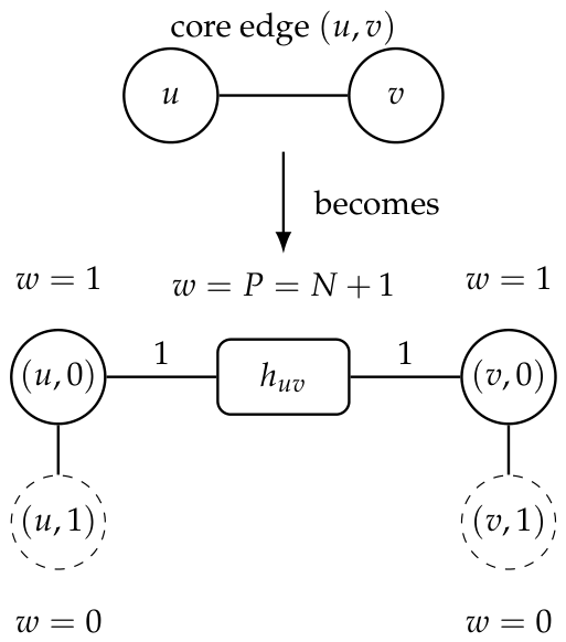
Figure 2.
Oriented-incidence gadget of a vertex u with unprocessed neighbours: an even cycle . Solid forcing edges encode the original edges ; dashed local edges close the cycle. Blue nodes (weight ) decode to u, orange nodes (weight ) to .
Figure 2.
Oriented-incidence gadget of a vertex u with unprocessed neighbours: an even cycle . Solid forcing edges encode the original edges ; dashed local edges close the cycle. Blue nodes (weight ) decode to u, orange nodes (weight ) to .
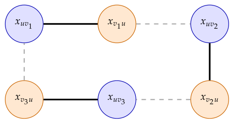
Figure 3.
The edge-dominating-set gadget of . Left: a graph G in which u has neighbours (adjacency order) and are adjacent. Right: its gadget D. Every edge of G is an edge-node (grey box); every vertex receives incidence nodes (circles) that thread its edge-nodes into a path, e.g. for u, while v, of degree 1, has the single node . The incidence index k in is a position on the path of u, never a neighbour. The thick red edges are all the path edges of the vertices labelled 1, u and z (shaded): they form an edge dominating set of D, since every gadget edge shares an endpoint with one of them, and they decode to the cover . Its weight is : one unit per vertex, and an overlap of 1 because the edge has both endpoints in the cover. Every minimum cover of G ( or ) has this weight, and no other labelling is lighter.
Figure 3.
The edge-dominating-set gadget of . Left: a graph G in which u has neighbours (adjacency order) and are adjacent. Right: its gadget D. Every edge of G is an edge-node (grey box); every vertex receives incidence nodes (circles) that thread its edge-nodes into a path, e.g. for u, while v, of degree 1, has the single node . The incidence index k in is a position on the path of u, never a neighbour. The thick red edges are all the path edges of the vertices labelled 1, u and z (shaded): they form an edge dominating set of D, since every gadget edge shares an endpoint with one of them, and they decode to the cover . Its weight is : one unit per vertex, and an overlap of 1 because the edge has both endpoints in the cover. Every minimum cover of G ( or ) has this weight, and no other labelling is lighter.
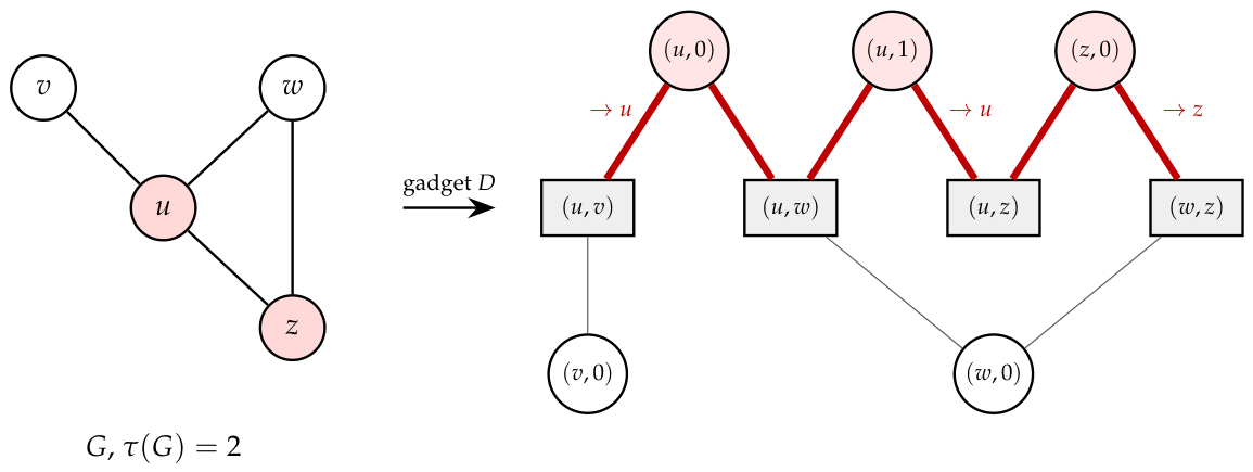
Table 1.
Code metadata for the Salvador package (v0.1.1).
| Nr. | Code metadata description | Metadata |
|---|---|---|
| C1 | Current code version | v0.1.1 |
| C2 | Permanent link to code repository | https://github.com/frankvegadelgado/salvador |
| C3 | Permanent link to reproducible capsule | https://pypi.org/project/salvador/ |
| C4 | Legal Code License | MIT License |
| C5 | Code versioning system used | git |
| C6 | Languages, tools, and services used | Python , NetworkX , NumPy , SciPy |
| C7 | Compilation requirements and dependencies | Python, NetworkX, NumPy, SciPy |
Table 2.
Winning strategy, proved ratio and observed ratio by graph class, at the target ratio . Rows marked “no” and “open” contain graphs of the nearly Konig–Egerváry residue of Section 5.13; rows marked “per instance” are covered by Theorem 8 on their instances with , and on every instance by the a-posteriori certificate of Theorem 13, which proves the ratio of the returned cover from a maximum fractional matching. Observed values are the largest measured on families of that kind.
Table 2.
Winning strategy, proved ratio and observed ratio by graph class, at the target ratio . Rows marked “no” and “open” contain graphs of the nearly Konig–Egerváry residue of Section 5.13; rows marked “per instance” are covered by Theorem 8 on their instances with , and on every instance by the a-posteriori certificate of Theorem 13, which proves the ratio of the returned cover from a maximum fractional matching. Observed values are the largest measured on families of that kind.
| Graph class | Winner | Proved ratio | ? | Observed |
|---|---|---|---|---|
| Trees, forests, stars | (leaf rule), | 1 (Thm. 4) | yes | |
| Paths, cycles (max. deg. 2) | 1 (Thm. 4) | yes | ||
| Complete graphs | 1 (Thm. 4) | yes | ||
| Complete bipartite | , | 1 (Thms. 4, 6) | yes | |
| Regular bipartite, every degree | , | 1 (Thm. 6) | yes | (Parts D, G) |
| Degree-separated bipartite | , | 1 (Thm. 6) | yes | |
| d-regular, | , , then | (Thm. 5) | yes | () |
| (near-regular) | , then | (Cor. 1) | yes | |
| Any graph | (residual) | (Lem. 6) | per instance | |
| Crown graphs, every h | , | 1 (Thm. 6) | yes | |
| d-reg., | every candidate | (Cor. 3) | yes | |
| d-reg., , non-bip., | , then | no | not tested | |
| (any degree) | , | (Thm. 8) | yes | |
| , clique factors | every candidate | (Cor. 3) | yes | |
| Max. degree , irregular | (Thm. 9) | yes | ||
| Hub-dominated, Thm. 10 | yes | |||
| Bipartite, , other | , , | 2 a priori; a posteriori (Thm. 13) | per instance | (Part D) |
| Bipartite, empty core | , | 1 (Prop. 4, Thm. 11) | yes | |
| Khot–Regev YES-type | , then | 2 a priori; a posteriori | per instance | (Part E) |
| Planar grids | , , | 2 | no | |
| Sparse Erdos–Rényi | or , then | per instance | ||
| Barabási–Albert | or , then | per instance | ||
| Watts–Strogatz | or , then | per instance | ||
| DIMACS clique complements | best of | per instance | ||
| All graphs | (refined ) | 2 (Thm. 2) | open (Conj. 2) |
Table 3.
Guarantees and limitations of the individual strategies. The combined algorithm satisfies the best applicable bound among the strategies (Thm. 12).
Table 3.
Guarantees and limitations of the individual strategies. The combined algorithm satisfies the best applicable bound among the strategies (Thm. 12).
| Strategy | Guarantee and limitation |
|---|---|
| matching | , ratio (Thm. 8). The a-priori bound is 2 when ; there the a-posteriori bound is exact (Thm. 13). |
| max-degree | Ratio at most for (Thm. 9); minimal (Thm. 7). For , no bound strictly below 2 is proved. |
| Hallelujah | (Thm. 10); ratio at most on regular components (Prop. 3). On d-regular graphs, . |
| Min-to-Min | Exact on forests, graphs with , , (Thm. 4), and regular or degree-separated bipartite graphs (Thm. 6). Outside these classes, arbitrary neighbour choices are possible when . |
| primal-dual | Same guarantee as on unweighted graphs; inherits its limitations. |
| MIDS forest core | Minimal (Thm. 7); ratio 2. No stronger guarantee for a separate graph class is established. |
| union re-prune | Minimal; no larger than any of . No independent guarantee beyond those inherited from preceding strategies. |
| bipartite planar | Caro–Wei bound (Lemma 6); ratio at most (Cor. 1); exact on regular and degree-separated bipartite graphs (Thm. 6). |
| -swap ILS | Never worse than . No independent approximation ratio is proved; depends on budgeted local search. |
| EDS + DP | Minimum vertex cover with fewest doubly covered edges on bipartite components with empty core (Prop. 4); never worse than ; bags of at most six nodes, so the core is non-empty when the gadget has treewidth above 5. |
| treewidth DP | Exact when the core is empty (Thm. 11); treewidth cap 10. |
| swap-maximize | Never worse than its input (Prop. 5); inherits the guarantee of its input. |
Table 4.
Part A: ratio of the returned cover to the exact optimum, by family. Every one of the instances was solved exactly () and every returned cover was valid.
Table 4.
Part A: ratio of the returned cover to the exact optimum, by family. Every one of the instances was solved exactly () and every returned cover was valid.
| Family | Instances | Mean ratio | Max ratio |
|---|---|---|---|
| Graph atlas () | 1245 | 1.000 | 1.000 |
| Bipartite hill-climb (exact) | 80 | 1.000 | 1.000 |
| Random general (exact, ) | 173 | 1.000 | 1.000 |
| Random bipartite (exact) | 99 | 1.000 | 1.000 |
| Grids, bipartite (exact) | 64 | 1.000 | 1.000 |
| Relabel / order stress (exact) | 56 | 1.000 | 1.000 |
| Bipartite obstruction (exact) | 1 | 1.000 | 1.000 |
| Overall | 1718 | 1.000 | 1.000 |
Table 5.
Part B (v0.1.1): certified ratio upper bound on the 26 instances of the ten large/adversarial families (up to vertices and edges), the lower-bound method that attained it, the bound the greedy maximal matching alone would give, and the wall-clock time of the largest instance solved. Every returned cover was valid.
Table 5.
Part B (v0.1.1): certified ratio upper bound on the 26 instances of the ten large/adversarial families (up to vertices and edges), the lower-bound method that attained it, the bound the greedy maximal matching alone would give, and the wall-clock time of the largest instance solved. Every returned cover was valid.
| Family | Max n | Max ratio u.b. | Bound | Matching-only | Max time (s) |
|---|---|---|---|---|---|
| Random 12-regular | 50,000 | 1.168 | spectral | 1.574 | 26.22 |
| Random 6-regular | 200,000 | 1.145 | spectral | 1.416 | 85.87 |
| Random 3-regular | 200,000 | 1.079 | spectral | 1.248 | 45.56 |
| Sparse Erdos–Renyi (deg. 4) | 50,000 | 1.066 | Karp–Sipser | 1.257 | 10.96 |
| Watts–Strogatz small-world | 50,000 | 1.055 | clique packing | 1.418 | 10.21 |
| Barabasi–Albert scale-free | 200,000 | 1.011 | Karp–Sipser | 1.353 | 78.94 |
| Complete bipartite | 1,600 | 1.000 | exact | 1.000 | 105.92 |
| Crown graph | 1,600 | 1.000 | exact | 1.000 | 101.93 |
| Double star + bridge | 200,002 | 1.000 | exact | 1.000 | 55.69 |
| Hierarchical star trap | 152,917 | 1.000 | exact | 1.000 | 43.11 |
Table 6.
Salvador (v0.1.1) and Hvala on the 68 DIMACS clique-complement instances of NPBench [29] — Part 1 of 2 (brock, c-fat, C, gen, hamming). Hvala figures are those reported in [11]; Salvador figures come from the raw log of a single run. Ratio is the cover size divided by the known optimum (OPT). †: best-known upper bound on (maximum clique not confirmed optimal [30]); the ratio is then a lower bound.
Table 6.
Salvador (v0.1.1) and Hvala on the 68 DIMACS clique-complement instances of NPBench [29] — Part 1 of 2 (brock, c-fat, C, gen, hamming). Hvala figures are those reported in [11]; Salvador figures come from the raw log of a single run. Ratio is the cover size divided by the known optimum (OPT). †: best-known upper bound on (maximum clique not confirmed optimal [30]); the ratio is then a lower bound.
| Cover size | Time | Ratio | |||||
|---|---|---|---|---|---|---|---|
| Instance | OPT | Hvala | Salvador | Hvala | Salvador | Hvala | Salvador |
| brock200_1 | 179 | 183 | 180 | 65.5ms | 188.2ms | 1.022 | 1.006 |
| brock200_2 | 188 | 192 | 190 | 233.3ms | 347.0ms | 1.021 | 1.011 |
| brock200_3 | 185 | 189 | 187 | 291.4ms | 279.4ms | 1.022 | 1.011 |
| brock200_4 | 183 | 187 | 184 | 92.0ms | 242.2ms | 1.022 | 1.005 |
| brock400_1 | 373 | 381 | 376 | 450.0ms | 764.0ms | 1.021 | 1.008 |
| brock400_2 | 371 | 379 | 377 | 500.5ms | 685.0ms | 1.022 | 1.016 |
| brock400_3 | 369 | 381 | 377 | 441.7ms | 750.2ms | 1.033 | 1.022 |
| brock400_4 | 367 | 378 | 376 | 507.7ms | 656.7ms | 1.030 | 1.025 |
| brock800_1 | 777 | 785 | 781 | 3.96s | 3.91s | 1.010 | 1.005 |
| brock800_2 | 776 | 783 | 780 | 4.13s | 3.97s | 1.009 | 1.005 |
| brock800_3 | 775 | 784 | 781 | 4.20s | 3.94s | 1.012 | 1.008 |
| brock800_4 | 774 | 785 | 781 | 4.53s | 4.33s | 1.014 | 1.009 |
| c-fat200-1 | 188 | 188 | 188 | 383.7ms | 495.9ms | 1.000 | 1.000 |
| c-fat200-2 | 176 | 176 | 176 | 790.0ms | 383.3ms | 1.000 | 1.000 |
| c-fat200-5 | 142 | 142 | 142 | 251.1ms | 426.0ms | 1.000 | 1.000 |
| c-fat500-1 | 486 | 486 | 486 | 3.87s | 4.55s | 1.000 | 1.000 |
| c-fat500-10 | 374 | 374 | 374 | 2.74s | 3.43s | 1.000 | 1.000 |
| c-fat500-2 | 474 | 474 | 474 | 3.75s | 5.83s | 1.000 | 1.000 |
| c-fat500-5 | 436 | 436 | 436 | 3.68s | 4.49s | 1.000 | 1.000 |
| C1000.9 | 932† | 945 | 937 | 1.87s | 1.88s | 1.014 | 1.005 |
| C125.9 | 91 | 92 | 91 | 174.7ms | 47.5ms | 1.011 | 1.000 |
| C250.9 | 206 | 214 | 206 | 60.8ms | 146.4ms | 1.039 | 1.000 |
| C500.9 | 443 † | 454 | 446 | 336.5ms | 495.0ms | 1.025 | 1.007 |
| gen200_p0.9_44 | 156 | 167 | 160 | 32.9ms | 108.0ms | 1.071 | 1.026 |
| gen200_p0.9_55 | 145 | 163 | 159 | 82.6ms | 89.9ms | 1.124 | 1.097 |
| gen400_p0.9_55 | 345 | 356 | 349 | 192.7ms | 395.9ms | 1.032 | 1.012 |
| gen400_p0.9_65 | 335 | 359 | 351 | 183.1ms | 475.1ms | 1.072 | 1.048 |
| gen400_p0.9_75 | 325 | 358 | 347 | 166.9ms | 767.1ms | 1.102 | 1.068 |
| hamming10-2 | 512 | 512 | 512 | 72.1ms | 1.41s | 1.000 | 1.000 |
| hamming10-4 | 984 | 992 | 986 | 6.43s | 5.62s | 1.008 | 1.002 |
| hamming6-2 | 32 | 32 | 32 | 11.7ms | 63.5ms | 1.000 | 1.000 |
| hamming6-4 | 60 | 60 | 60 | 50.5ms | 63.9ms | 1.000 | 1.000 |
| hamming8-2 | 128 | 128 | 128 | 442.0ms | 240.0ms | 1.000 | 1.000 |
| hamming8-4 | 240 | 240 | 240 | 599.7ms | 514.4ms | 1.000 | 1.000 |
Table 7.
Salvador (v0.1.1) and Hvala on the 68 DIMACS clique-complement instances of NPBench [29] — Part 2 of 2 (johnson, keller, MANN, p_hat, san, sanr). Hvala figures are those reported in [11]; Salvador figures come from the raw log of a single run. Ratio is the cover size divided by the known optimum (OPT).
Table 7.
Salvador (v0.1.1) and Hvala on the 68 DIMACS clique-complement instances of NPBench [29] — Part 2 of 2 (johnson, keller, MANN, p_hat, san, sanr). Hvala figures are those reported in [11]; Salvador figures come from the raw log of a single run. Ratio is the cover size divided by the known optimum (OPT).
| Cover size | Time | Ratio | |||||
|---|---|---|---|---|---|---|---|
| Instance | OPT | Hvala | Salvador | Hvala | Salvador | Hvala | Salvador |
| johnson16-2-4 | 112 | 112 | 112 | 83.3ms | 128.5ms | 1.000 | 1.000 |
| johnson32-2-4 | 480 | 480 | 480 | 827.6ms | 1.02s | 1.000 | 1.000 |
| johnson8-2-4 | 24 | 24 | 24 | 2.9ms | 0.0ms | 1.000 | 1.000 |
| johnson8-4-4 | 56 | 56 | 56 | 32.3ms | 21.1ms | 1.000 | 1.000 |
| keller4 | 160 | 162 | 160 | 348.8ms | 497.8ms | 1.012 | 1.000 |
| keller5 | 749 | 759 | 751 | 4.96s | 4.93s | 1.013 | 1.003 |
| MANN_a27 | 252 | 253 | 253 | 35.7ms | 50.7ms | 1.004 | 1.004 |
| MANN_a45 | 690 | 695 | 693 | 145.5ms | 148.1ms | 1.007 | 1.004 |
| MANN_a81 | 2221 | 2225 | 2224 | 769.8ms | 575.3ms | 1.002 | 1.001 |
| MANN_a9 | 29 | 29 | 29 | 6.6ms | 17.0ms | 1.000 | 1.000 |
| p_hat1000-3 | 932 | 942 | 935 | 9.60s | 7.53s | 1.011 | 1.003 |
| p_hat300-1 | 292 | 292 | 292 | 2.43s | 1.16s | 1.000 | 1.000 |
| p_hat300-2 | 275 | 277 | 275 | 1.38s | 814.4ms | 1.007 | 1.000 |
| p_hat300-3 | 264 | 268 | 266 | 735.5ms | 409.8ms | 1.015 | 1.008 |
| p_hat500-1 | 491 | 492 | 491 | 6.29s | 6.00s | 1.002 | 1.000 |
| p_hat500-2 | 464 | 469 | 464 | 4.45s | 3.91s | 1.011 | 1.000 |
| p_hat500-3 | 450 | 454 | 451 | 2.30s | 1.82s | 1.009 | 1.002 |
| p_hat700-1 | 689 | 693 | 691 | 14.28s | 10.38s | 1.006 | 1.003 |
| p_hat700-2 | 656 | 658 | 656 | 9.51s | 6.48s | 1.003 | 1.000 |
| p_hat700-3 | 638 | 642 | 638 | 4.71s | 3.07s | 1.006 | 1.000 |
| san200_0.7_1 | 170 | 184 | 183 | 296.9ms | 277.7ms | 1.082 | 1.076 |
| san200_0.7_2 | 182 | 188 | 185 | 313.7ms | 343.1ms | 1.033 | 1.016 |
| san200_0.9_1 | 130 | 155 | 151 | 89.4ms | 143.6ms | 1.192 | 1.162 |
| san200_0.9_2 | 140 | 162 | 159 | 100.6ms | 152.7ms | 1.157 | 1.136 |
| san200_0.9_3 | 156 | 169 | 165 | 451.1ms | 170.3ms | 1.083 | 1.058 |
| san400_0.5_1 | 387 | 393 | 391 | 2.36s | 2.16s | 1.016 | 1.010 |
| san400_0.7_1 | 360 | 379 | 378 | 1.47s | 1.63s | 1.053 | 1.050 |
| san400_0.7_2 | 370 | 385 | 382 | 1.40s | 1.47s | 1.041 | 1.032 |
| san400_0.7_3 | 378 | 388 | 382 | 1.43s | 1.45s | 1.026 | 1.011 |
| san400_0.9_1 | 300 | 348 | 300 | 507.9ms | 614.2ms | 1.160 | 1.000 |
| sanr200_0.7 | 182 | 184 | 182 | 330.7ms | 348.7ms | 1.011 | 1.000 |
| sanr200_0.9 | 158 | 160 | 159 | 83.0ms | 196.3ms | 1.013 | 1.006 |
| sanr400_0.5 | 387 | 388 | 387 | 2.51s | 2.30s | 1.003 | 1.000 |
| sanr400_0.7 | 379 | 383 | 380 | 1.56s | 1.26s | 1.011 | 1.003 |
Table 9.
Part E: the final cover on 117 sampled Khot–Regev YES instances (640 to vertices). “≤ planted” counts the instances on which is at most the planted cover; “ known” those on which an integer program proved the optimum within 90 seconds; the base family has , , , , ; “Max exact” is the largest ratio where is known; “Max cert.” is the largest value of , where L is the best certified lower bound (integer-program bound or linear relaxation), an upper bound on the true ratio.
Table 9.
Part E: the final cover on 117 sampled Khot–Regev YES instances (640 to vertices). “≤ planted” counts the instances on which is at most the planted cover; “ known” those on which an integer program proved the optimum within 90 seconds; the base family has , , , , ; “Max exact” is the largest ratio where is known; “Max cert.” is the largest value of , where L is the best certified lower bound (integer-program bound or linear relaxation), an upper bound on the true ratio.
| Family | Inst. | ≤ planted | known | Optimal | Max exact | Max cert. |
|---|---|---|---|---|---|---|
| Base family | 12 | 8 | 3 | 1 | 1.0056 | 1.115 |
| Label size | 12 | 5 | 4 | 4 | 1.0000 | 1.141 |
| Label size | 12 | 12 | 6 | 6 | 1.0000 | 1.024 |
| Bias | 12 | 12 | 2 | 1 | 1.0391 | 1.237 |
| Bias | 12 | 11 | 6 | 4 | 1.0160 | 1.018 |
| Noise | 12 | 11 | 3 | 2 | 1.0089 | 1.105 |
| Noise | 12 | 12 | 3 | 2 | 1.0057 | 1.110 |
| Constraint degree | 12 | 8 | 6 | 4 | 1.0356 | 1.149 |
| Samples per block | 9 | 3 | 2 | 1 | 1.0232 | 1.175 |
| Linear UG, Max-2-Lin | 12 | 10 | 4 | 2 | 1.0425 | 1.106 |
| All | 117 | 92 | 39 | 27 | 1.0425 | 1.237 |
Table 10.
Part F: 120 instances, 140 to vertices. “Max exact” is the largest where is proved; “Max cert.” the largest with L the best certified lower bound; “Max ” the largest proved per-instance bound of Theorem 12; “Bias” the mean probability that a vertex of a maximum independent set (or of the planted or returned one, where is unknown) has smaller degree than a vertex outside it; “Greedy exc.” the mean relative excess of over . No returned cover admits a -swap.
Table 10.
Part F: 120 instances, 140 to vertices. “Max exact” is the largest where is proved; “Max cert.” the largest with L the best certified lower bound; “Max ” the largest proved per-instance bound of Theorem 12; “Bias” the mean probability that a vertex of a maximum independent set (or of the planted or returned one, where is unknown) has smaller degree than a vertex outside it; “Greedy exc.” the mean relative excess of over . No returned cover admits a -swap.
| Family | known | Opt. | Max exact | Max cert. | Max | Bias | Greedy exc. |
|---|---|---|---|---|---|---|---|
| KR sampled | 10/12 | 6 | 1.0058 | 1.0498 | 1.840 | 0.852 | 2.02% |
| KR sampled | 12/12 | 12 | 1.0000 | 1.0000 | 1.920 | 0.919 | 1.17% |
| KR fixed (bip.) | 12/12 | 7 | 1.0779 | 1.0779 | 2.000 | 0.616 | 4.54% |
| KR fixed | 6/12 | 4 | 1.0938 | 1.1376 | 1.776 | 0.517 | 6.09% |
| KR fixed (bip.) | 12/12 | 10 | 1.0038 | 1.0038 | 1.797 | 0.795 | 1.65% |
| Planted regular , | 9/12 | 9 | 1.0000 | 1.0495 | 1.651 | 0.600 | 0.13% |
| Planted regular , | 11/12 | 11 | 1.0000 | 1.0045 | 1.760 | 0.641 | 0.00% |
| Random regular | 6/12 | 3 | 1.0169 | 1.0804 | 1.457 | 0.500 | 3.10% |
| Random regular | 3/12 | 1 | 1.0095 | 1.2313 | 1.606 | 0.500 | 3.49% |
| Thinned grid (, bip.) | 12/12 | 7 | 1.0099 | 1.0099 | 1.460 | 0.641 | 2.97% |
| All | 93/120 | 70 | 1.0938 | 1.2313 | 2.000 | 0.658 | 2.27% |
Table 12.
Part F: mean ratio by size ( vertices for the Khot–Regev and regular families). Each entry averages the exact ratio where is proved and the certified bound elsewhere, so entries for large N on the regular families are upper bounds.
Table 12.
Part F: mean ratio by size ( vertices for the Khot–Regev and regular families). Each entry averages the exact ratio where is proved and the certified bound elsewhere, so entries for large N on the regular families are upper bounds.
| Family | ||||
|---|---|---|---|---|
| KR sampled | 1.0000 | 1.0018 | 1.0039 | 1.0315 |
| KR sampled | 1.0000 | 1.0000 | 1.0000 | 1.0000 |
| KR fixed | 1.0084 | 1.0281 | 1.0095 | 1.0000 |
| KR fixed | 1.0313 | 1.0052 | 1.0731 | 1.1251 |
| KR fixed | 1.0000 | 1.0000 | 1.0013 | 1.0006 |
| Planted regular , | 1.0000 | 1.0000 | 1.0000 | 1.0361 |
| Planted regular , | 1.0000 | 1.0000 | 1.0000 | 1.0015 |
| Random regular | 1.0000 | 1.0113 | 1.0461 | 1.0686 |
| Random regular | 1.0063 | 1.1056 | 1.1520 | 1.2103 |
| Thinned grid () | 1.0000 | 1.0000 | 1.0055 | 1.0045 |
Table 13.
Part G: random d-regular graphs. The columns to give the largest ratio over three seeds, exact for and certified (, spectral lower bound L) otherwise; and are means at ; “vs. estimate” is the mean of divided by the estimate of of random d-regular graphs [33], which is asymptotic in d and not a bound; the last column is the spectral a-priori bound for . On the 117 random regular bipartite graphs of the same degrees and sizes every returned cover is optimal.
Table 13.
Part G: random d-regular graphs. The columns to give the largest ratio over three seeds, exact for and certified (, spectral lower bound L) otherwise; and are means at ; “vs. estimate” is the mean of divided by the estimate of of random d-regular graphs [33], which is asymptotic in d and not a bound; the last column is the spectral a-priori bound for . On the 117 random regular bipartite graphs of the same degrees and sizes every returned cover is optimal.
| d | (exact) | vs. estimate | ||||||
|---|---|---|---|---|---|---|---|---|
| 3 | 1.0000 | 1.0769 | 1.0833 | 1.0812 | 0.556 | 0.515 | 2.077 | 1.943 |
| 4 | 1.0000 | 1.1204 | 1.1134 | 1.1115 | 0.596 | 0.536 | 1.941 | 1.866 |
| 5 | 1.0000 | 1.1339 | 1.1367 | 1.1331 | 0.630 | 0.556 | 1.768 | 1.800 |
| 6 | 1.0000 | 1.1466 | 1.1429 | 1.1441 | 0.655 | 0.574 | 1.627 | 1.745 |
| 8 | 1.0000 | 1.1653 | 1.1609 | 1.1594 | 0.698 | 0.602 | 1.453 | 1.661 |
| 10 | 1.0000 | 1.1587 | 1.1712 | 1.1676 | 0.730 | 0.626 | 1.352 | 1.600 |
| 12 | 1.0000 | 1.1603 | 1.1734 | 1.1694 | 0.753 | 0.645 | 1.285 | 1.553 |
| 16 | 1.0000 | 1.1606 | 1.1733 | 1.1705 | 0.789 | 0.675 | 1.207 | 1.484 |
| 20 | 1.0000 | 1.1549 | 1.1679 | 1.1715 | 0.815 | 0.697 | 1.164 | 1.436 |
| 24 | 1.0000 | 1.1507 | 1.1690 | 1.1692 | 0.835 | 0.715 | 1.136 | 1.400 |
| 32 | 1.0000 | 1.1589 | 1.1667 | 1.1605 | 0.861 | 0.743 | 1.099 | 1.348 |
| 48 | – | 1.1250 | 1.1443 | 1.1504 | 0.896 | 0.779 | 1.068 | 1.286 |
| 64 | – | 1.1145 | 1.1363 | 1.1403 | 0.915 | 0.803 | 1.051 | 1.248 |
Table 14.
Part H1: on its own, with the pruned cover of a maximal matching as reference, on 108 bipartite graphs with up to vertices. “Max bag” is the largest bag built; “Exact” counts the instances with an empty core; and “Ref.” are the means of the cover and of the reference over ; “Max tw LB” is the largest minor-min-width lower bound on the treewidth of the gadget. In the ensemble the reference is the best of instead, and is never worse than it.
Table 14.
Part H1: on its own, with the pruned cover of a maximal matching as reference, on 108 bipartite graphs with up to vertices. “Max bag” is the largest bag built; “Exact” counts the instances with an empty core; and “Ref.” are the means of the cover and of the reference over ; “Max tw LB” is the largest minor-min-width lower bound on the treewidth of the gadget. In the ensemble the reference is the best of instead, and is never worse than it.
| Family | Inst. | Max bag | Exact | Ref. | Max tw LB | Time (s) | |
|---|---|---|---|---|---|---|---|
| Random bipartite (balanced) | 18 | 3 | 0 | 1.656 | 1.821 | 69 | 6.23 |
| Random bipartite (1:2) | 18 | 4 | 0 | 1.798 | 1.984 | 46 | 5.99 |
| Random d-regular bipartite | 18 | 4 | 0 | 1.660 | 1.795 | 41 | 3.61 |
| Power-law bipartite | 6 | 3 | 0 | 1.068 | 1.837 | 17 | 0.67 |
| Double cover | 12 | 3 | 0 | 1.612 | 1.775 | 30 | 2.09 |
| Hidden perfect matching | 12 | 4 | 0 | 1.452 | 1.776 | 30 | 2.06 |
| Random tree | 6 | 2 | 6 | 1.000 | 1.783 | 1 | 0.48 |
| 2D grid, of edges | 6 | 6 | 2 | 1.110 | 1.905 | 5 | 1.98 |
| 2D grid | 2 | 4 | 0 | 1.697 | 1.978 | 7 | 0.40 |
| 3D grid | 2 | 3 | 0 | 1.939 | 1.994 | 15 | 0.42 |
| Even cycle | 2 | 3 | 2 | 1.000 | 2.000 | 2 | 0.30 |
| Complete bipartite | 2 | 4 | 0 | 2.000 | 2.000 | 5 | 29.27 |
| Crown graph | 2 | 5 | 0 | 2.000 | 2.000 | 6 | 41.40 |
| Hypercube | 1 | 3 | 0 | 1.953 | 1.953 | 19 | 0.11 |
| Hypercube, of edges | 1 | 3 | 0 | 1.609 | 1.859 | 12 | 0.06 |
| All | 108 | 6 | 10 | 95.07 |
Table 17.
The labelled, weighted edge-dominating-set strategy (bags of at most six nodes, ) on the instances of Table 15. “Empty core” means that the gadget was solved exactly, so that is a minimum vertex cover; “Decoded ≤ best” counts the instances on which the pruned decoded cover, before the fallback to the reference, is no larger than the best of . On non-bipartite graphs the decoded cover is the reference itself.
Table 17.
The labelled, weighted edge-dominating-set strategy (bags of at most six nodes, ) on the instances of Table 15. “Empty core” means that the gadget was solved exactly, so that is a minimum vertex cover; “Decoded ≤ best” counts the instances on which the pruned decoded cover, before the fallback to the reference, is no larger than the best of . On non-bipartite graphs the decoded cover is the reference itself.
| Family | Inst. | Bipartite | Empty core | Decoded ≤ best |
|---|---|---|---|---|
| Graph atlas () | 1245 | 142 | 142 | 1245 |
| Random general (exact, ) | 173 | 18 | 18 | 173 |
| Random bipartite (exact) | 99 | 99 | 94 | 99 |
| Grids, bipartite (exact) | 64 | 64 | 38 | 64 |
| Relabel / order stress (exact) | 56 | 56 | 56 | 56 |
| Double star, hierarchical star trap, obstruction | 4 | 4 | 4 | 4 |
| Complete bipartite, crown graph | 6 | 6 | 0 | 6 |
| Large non-bipartite families | 12 | 0 | 0 | 12 |
Table 19.
Strict improvements of the final refinement over the best of .
| Instance | Best of | Refined from | |
|---|---|---|---|
| Random 3-regular, | 2,779 | 2,778 | , , |
| Random 12-regular, | 3,758 | 3,757 | , , |
| Random 3-regular, | 27,749 | 27,748 | |
| Random 6-regular, | 32,808 | 32,807 | , , |
| Random 12-regular, | 37,630 | 37,629 | , , |
| Sparse Erdos–Renyi, | 26,096 | 26,095 | , , |
| Watts–Strogatz, | 35,439 | 35,438 |
Disclaimer/Publisher’s Note: The statements, opinions and data contained in all publications are solely those of the individual author(s) and contributor(s) and not of MDPI and/or the editor(s). MDPI and/or the editor(s) disclaim responsibility for any injury to people or property resulting from any ideas, methods, instructions or products referred to in the content. |
© 2026 by the authors. Licensee MDPI, Basel, Switzerland. This article is an open access article distributed under the terms and conditions of the Creative Commons Attribution (CC BY) license (http://creativecommons.org/licenses/by/4.0/).
Copyright: This open access article is published under a Creative Commons CC BY 4.0 license, which permit the free download, distribution, and reuse, provided that the author and preprint are cited in any reuse.