An Approximate Solution to the Minimum Vertex Cover Problem: The Salvador Algorithm

1. Introduction

The Minimum Vertex Cover (VC) problem is one of the twenty-one NP-complete problems identified by Karp [1]. Given an undirected graph $G=(V,E)$, a set $C\subseteq V$ is a vertex cover if every edge of E has at least one endpoint in C; the goal is to find a minimum-cardinality vertex cover, denoted $\tau \left(G\right)$. Vertex cover is central to computer science, modelling guard placement, network monitoring, error-correcting codes, and serving as the canonical starting point for parameterised and approximation algorithms.

The approximation landscape for VC is unusually well charted. The classical maximal-matching algorithm achieves a 2-approximation in linear time [2]; LP-based refinements by Karakostas [3] and Karpinski and Zelikovsky [4] reach factor $2-\Theta (1/\sqrt{logn})$, which is $2-o\left(1\right)$ but falls short of a constant $2-\epsilon$. From the hardness side, Dinur and Safra [5] ruled out any ratio below $10\sqrt{5}-21\approx 1.3606$ under $\mathrm{P}\ne \mathrm{NP}$; subsequently, Khot, Minzer, and Safra [6,7,8] proved the 2-to-2 games conjecture, strengthening this barrier to $\sqrt{2}-\epsilon$ for any fixed $\epsilon >0$ under $\mathrm{P}\ne \mathrm{NP}$; and under the Unique Games Conjecture [9], no constant ratio below $2-\epsilon$ is achievable [10]. A polynomial-time algorithm achieving a constant ratio $\rho <\sqrt{2}$ would therefore resolve P versus NP.

Against this backdrop, we present an algorithm—implemented as the Salvador Python package (v0.0.3)—that, on the logged NPBench clique-complement instances, produces vertex covers with displayed ratios at most $1.192$ against the DIMACS reference values. The algorithm, called FindVertexCover, operates in three phases.

1.

Preprocessing. Self-loops are discarded; isolated vertices are removed (they appear in no edge and need not be covered).

2.

Bipartite planar reduction and weighted solve. For every connected component, the core routine constructs a weighted oriented-incidence auxiliary graph B. Each original edge $\{u,v\}$ creates an auxiliary edge between the incidence nodes $x_{uv}$ and $x_{vu}$; local consistency edges complete the planar bipartite gadget. Salvador then solves weighted vertex cover exactly on B by the integral bipartite LP/min-cut formulation.

3.

Linear-time pruning.PruneRedundantVertices makes a single forward pass over the candidate cover C and removes every vertex all of whose neighbours are already covered, reducing $\left|C\right|$ without compromising validity.

The construction and pruning phases are linear in the input and auxiliary sizes. The dominant step is the bipartite weighted vertex-cover solve on the planar auxiliary graph, which costs $O\left({\widehat{n}}^{3/2}\right)$ when $\widehat{n}=\left|V\left(B\right)\right|$ because $\left|E\left(B\right)\right|=O\left(\widehat{n}\right)$ for planar graphs. When the auxiliary incidence size is linear in the original graph size, this is $O\left(n^{3/2}\right)$.

1.0.0.1. Contributions

The main contributions of this paper are:

• A practical polynomial-time vertex-cover heuristic based on a weighted bipartite planar auxiliary reduction and an exact min-cut solve on the reduced instance.
• A TikZ-specified gadget that makes explicit how oriented incidences encode an original edge and local consistency around a vertex.
• An experimental study on 52 logged NPBench clique-complement benchmark graphs showing displayed ratios in $[1.000,1.192]$ (mean $1.042$).
• A conjecture that the universal approximation ratio is at most $1.4=\sqrt{2}-{\epsilon }_0$ for the explicit constant ${\epsilon }_0=\sqrt{2}-\frac{7}{5}\approx 0.0142>0$. Since $1.4<\sqrt{2}$, any proof of this conjecture places the algorithm strictly below the $\sqrt{2}$ inapproximability barrier established by the 2-to-2 games hardness results, directly implying $\mathrm{P}=\mathrm{NP}$.
• An open-source implementation, Salvador v0.0.3.

The paper is organised as follows. Section 3 describes the algorithm and provides pseudocode. Section 4 proves correctness. Section 5 analyses the approximation ratio and discusses consequences for $\mathrm{P}$ vs $\mathrm{NP}$. Section 6 establishes the time complexity. Section 7 reports the experimental results. Section 8 concludes.

2. Research Data

The algorithm is implemented in the Python package Salvador, freely available on the Python Package Index [11]. The current version is v0.0.3; code metadata is summarised in Table 1.

3. Description of the Algorithm

We present the pseudocode for the three components of the Salvador algorithm.

3.1. Main Algorithm

Algorithm 1 is the entry point. After cleaning the graph it solves each connected component through the bipartite planar auxiliary reduction and then applies the pruning pass to the union of the decoded component covers.

Algorithm 1:FindVertexCover$\left(G\right)$

Require:  Undirected graph $G=(V,E)$ Ensure:  A vertex cover $C\subseteq V$ 1: Remove all self-loops from G 2: $G\leftarrow G\setminus \{v\in V:{deg}_G\left(v\right)=0\}$▹ isolated vertices are in no edge 3: if$E=\varnothing$thenreturn∅ 4: end if 5: $C\leftarrow \varnothing$ 6: for each connected component $G_i$ of G do 7:     $C_i\leftarrow ComponentCover\left(G_i\right)$ 8:     $C\leftarrow C\cup C_i$ 9: end for 10: $\mathit{adj}\leftarrow \{v\mapsto N_G\left(v\right):v\in V\}$ 11: $C\leftarrow PruneRedundantVertices(\mathit{adj},C)$ 12: returnC

3.2. Bipartite Planar Gadget and Weighted Solve

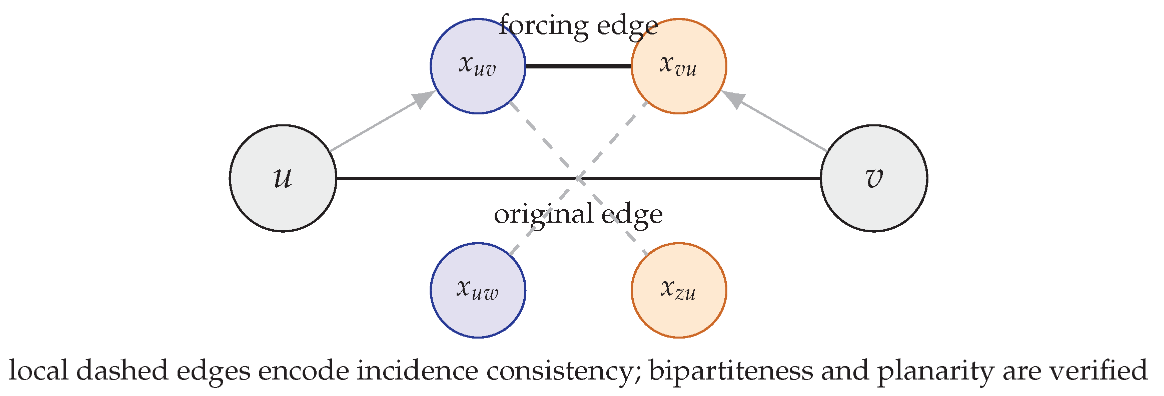
Algorithm 2 implements the component-level reduction used by Salvador. The routine processes a mutable copy of the component, so each original edge $\{u,v\}$ is handled exactly once, at which point it creates the two oriented-incidence nodes $x_{uv}$ and $x_{vu}$ with weights $1/{deg}_G\left(u\right)$ and $1/{deg}_G\left(v\right)$. The forcing edge $\{x_{uv},x_{vu}\}$ encodes the original edge, while local cyclic edges couple consecutive oriented incidences in the processing order. The implementation verifies that the resulting auxiliary graph is bipartite and planar before calling the exact weighted bipartite vertex-cover solver.

Algorithm 2:ComponentCover$\left(G_i\right)$

Require:  Connected component $G_i=(V_i,E_i)$ Ensure:  A vertex cover $C_i\subseteq V_i$ 1: $B\leftarrow \mathrm{new}\mathrm{graph}$ 2: $W\leftarrow \mathrm{mutable}\mathrm{copy}\mathrm{of}{G}_i$ 3: for$u\in V_i$do 4:     $(v_1,\dots ,v_d)\leftarrow N_W\left(u\right)$ 5:     Remove u from W 6:     $\mathit{first}\leftarrow \perp$;   $\mathit{prev}\leftarrow \perp$ 7:     for $j=1,\dots ,d$ do 8:         Add nodes $x_{u{v}_j}$ and $x_{v_{j}u}$ to B 9:         Set weights $w\left(x_{u{v}_j}\right)=1/{deg}_{G_i}\left(u\right)$ and $w\left(x_{v_{j}u}\right)=1/{deg}_{G_i}\left(v_j\right)$ 10:         Add forcing edge $\{x_{u{v}_j},x_{v_{j}u}\}$ to B 11:         if $\mathit{prev}=\perp$ then 12:            $\mathit{first}\leftarrow x_{u{v}_j}$ 13:         else 14:            Add local edge $\{x_{u{v}_j},\mathit{prev}\}$ to B 15:         end if 16:         $\mathit{prev}\leftarrow x_{v_{j}u}$ 17:     end for 18:     if $d>1$ then 19:         Add local edge $\{\mathit{first},\mathit{prev}\}$ to B 20:     end if 21: end for 22: ifB is not bipartite or not planar then 23:     raise reduction failure 24: end if 25: $S\leftarrow MinWeightVertexCoverBipartite\left(B\right)$▹ exact min-cut solve 26: $C_i\leftarrow \{u\in V_i:x_{uv}\in S\mathrm{for}\mathrm{some}\mathrm{auxiliary}\mathrm{node}{x}_{uv}\}$ 27: return$C_i$

The weighted solve is exact on B: the vertex-cover linear program is integral on bipartite graphs, equivalently by Konig’s theorem [12] and the max-flow/min-cut theorem. The selected auxiliary cover is then decoded by first coordinate. The forcing edge $\{x_{uv},x_{vu}\}$ is the key correctness device: covering it forces the decoded solution to contain u or v.

Figure 1. Bipartite planar reduction gadget. The original edge $\{u,v\}$ becomes the forcing edge $\{x_{uv},x_{vu}\}$ in the auxiliary graph. Any vertex cover of the auxiliary graph selects at least one endpoint of this forcing edge; decoding by first coordinate therefore selects u or v in the original graph.

Figure 1. Bipartite planar reduction gadget. The original edge $\{u,v\}$ becomes the forcing edge $\{x_{uv},x_{vu}\}$ in the auxiliary graph. Any vertex cover of the auxiliary graph selects at least one endpoint of this forcing edge; decoding by first coordinate therefore selects u or v in the original graph.

3.3. Linear-Time Pruning

Algorithm 3 removes redundant vertices from a candidate cover in a single forward pass, running in $O(n+m)$ total time.

Algorithm 3:PruneRedundantVertices$(\mathit{adj},C)$

Require:  Adjacency map $\mathit{adj}$, candidate cover $C\subseteq V$ Ensure:  Valid vertex cover $C^{\prime }\subseteq C$ with no redundant vertex 1: $C\leftarrow \mathrm{mutable}\mathrm{copy}\mathrm{of}C$ 2: for$v\in C$(in iteration order) do 3:     if $N_G\left(v\right)\subseteq C$then▹ every neighbour of v already covered by another member 4:         $C\leftarrow C\setminus \left\{v\right\}$ 5:     end if 6: end for 7: returnC

4. Correctness of the Algorithm

Theorem 1.  

Algorithm 1 always returns a valid vertex cover of the input graph G.

Proof. 

We must show that every edge $(u,v)\in E$ has at least one endpoint in the output C. Isolated vertices are removed in preprocessing and appear in no edge, so they need not be covered.

Component solve. Consider one connected component $G_i$ and any original edge $\{u,v\}\in E_i$. Algorithm 2 adds the forcing edge $\{x_{uv},x_{vu}\}$ to the auxiliary graph B. The set S returned by MinWeightVertexCoverBipartite is a vertex cover of B, so at least one of $x_{uv}$ and $x_{vu}$ lies in S. If $x_{uv}\in S$, the decoder places u in $C_i$; if $x_{vu}\in S$, it places v in $C_i$. Hence every edge of $G_i$ is covered by $C_i$.

Union over components. Distinct connected components have no edges between them. Therefore the union $C={\bigcup }_i{C}_i$ covers all edges of the cleaned graph.

Pruning. A vertex $v\in C$ is removed by Algorithm 3 only when every neighbour of v lies in C. In that case every edge incident to v is already covered by the neighbour side, so removing v leaves every edge covered.    □

5. Approximation Ratio and Consequences for P vs NP

5.1. What Is Proved and What Is Conjectured

Let $G=(V,E)$ be the input graph. Write $\tau \left(G\right)$ for the size of a minimum vertex cover of G, and let $C_S\left(G\right)$ be the cover returned by Algorithm 1. The correctness theorem proves that $C_S\left(G\right)$ is always feasible whenever the bipartite planar reduction succeeds. The weighted auxiliary objective is a surrogate objective: Salvador solves the weighted vertex-cover problem exactly on the auxiliary graph B, but the decoded cardinality $|C_S\left(G\right)|$ is not claimed here to be exactly equal to $\tau \left(G\right)$.

The approximation statement studied in this paper is therefore the ratio

$$R_S\left(G\right)={\displaystyle \frac{|C_S\left(G\right)|}{\tau \left(G\right)}}.$$

For the logged DIMACS clique-complement instances, $\tau \left(G\right)$ is computed as $n-\omega \left(G_0\right)$ from the published clique number of the original DIMACS graph $G_0$; rows marked † use a best-known clique lower bound and therefore give a displayed reference ratio rather than a certified ratio.

5.2. The $1.4$ Conjecture and the $\sqrt{2}$ Inapproximability Threshold

The following algebraic observation is central to the paper’s main theoretical consequence.

Proposition 1  

($1.4=\sqrt{2}-{\epsilon }_0$). The value $\frac{7}{5}=1.4$ satisfies $\frac{7}{5}=\sqrt{2}-{\epsilon }_0$ for the positive constant ${\epsilon }_0=\sqrt{2}-\frac{7}{5}\approx 0.0142>0$. In particular, $1.4<\sqrt{2}$.

Proof. 

Direct computation: $\sqrt{2}\approx 1.41421$ and $7/5=1.4$, so ${\epsilon }_0=\sqrt{2}-7/5>0$.    □

Empirically, across the 52 logged NPBench benchmark instances in np_bench.txt, the displayed ratio $|C_S|/{\tau }^{*}$ lies in $[1.000,1.192]$ with mean $1.042$ (Section 7). Eleven logged instances are solved to the displayed optimum. We formalise the empirical finding as a conjecture.

Conjecture 1  

(Universal $1.4$-approximation). For every undirected graph G, the Salvador bipartite planar reduction succeeds and Algorithm 1 returns a vertex cover $C_S\left(G\right)$ with

$$|C_S\left(G\right)|\le \frac{7}{5}\tau \left(G\right)=(\sqrt{2}-{\epsilon }_0)\tau \left(G\right),$$

where ${\epsilon }_0=\sqrt{2}-\frac{7}{5}>0$.

Conjecture 1 is conservative relative to the current benchmark log: the largest displayed ratio observed is $1.192<1.4$. The value $1.4$ is the algebraically natural threshold because $1.4=\sqrt{2}-{\epsilon }_0$ places the conjectured ratio strictly below$\sqrt{2}$.

5.3. Consequences for P vs NP

Theorem 2  

(Implication for $\mathrm{P}$ vs $\mathrm{NP}$). If Algorithm 1 achieves an approximation ratio at most $1.4=\sqrt{2}-{\epsilon }_0$ on every undirected graph, then $\mathrm{P}=\mathrm{NP}$.

Proof. 

Khot, Minzer, and Safra [6,7,8] proved the 2-to-2 games conjecture and derived from it that, for every $\delta >0$, approximating Minimum Vertex Cover within a factor of $(\sqrt{2}-\delta )$ is NP-hard. Since $1.4=\sqrt{2}-{\epsilon }_0$ with ${\epsilon }_0=\sqrt{2}-\frac{7}{5}>0$, the ratio $1.4$ is exactly of the form $\sqrt{2}-\delta$ for $\delta ={\epsilon }_0$. Algorithm 1 runs in polynomial time (Theorem 3). A universal ratio $\le 1.4$ by this algorithm therefore constitutes a polynomial-time $(\sqrt{2}-{\epsilon }_0)$-approximation, contradicting the 2-to-2 games NP-hardness result unless $\mathrm{P}=\mathrm{NP}$.    □

Remark 1.  

Theorem 2 is a conditional implication: the missing ingredient is a proof of the universal ratio bound. The implication itself does not rely on the Unique Games Conjecture. Three layers of evidence motivate Conjecture 1: (i) Theorem 1 establishes feasibility of every returned cover; (ii) on every logged instance the displayed ratio lies in $[1.000,1.192]\subset [1,1.4)$, with the maximum already below the weaker Dinur–Safra threshold $10\sqrt{5}-21\approx 1.3606$ [5]; (iii) the explicit constant ${\epsilon }_0\approx 0.0142$ makes the conjecture algebraically precise rather than asymptotic. Under the Unique Games Conjecture, Khot and Regev [10] showed the stronger $2-\delta$ hardness barrier; a proved universal ratio of $1.4<2$ would also conflict with that conjectural barrier.

6. Runtime Analysis

Theorem 3.  

Let $G=(V,E)$ be the input graph, and let B be the disjoint union of the bipartite planar auxiliary graphs constructed across all connected components. Put $\widehat{n}=\left|V\left(B\right)\right|$ and $\widehat{m}=\left|E\left(B\right)\right|$. Algorithm 1 runs in

$$O\left(\right|V|+|E|+\widehat{m}\sqrt{\widehat{n}})$$

time. Since B is planar, $\widehat{m}=O\left(\widehat{n}\right)$, so the auxiliary solve is $O\left({\widehat{n}}^{3/2}\right)$. Writing n for the reduced auxiliary size gives the advertised $O\left(n^{3/2}\right)$ bound.

Proof. 

Preprocessing removes self-loops and isolated vertices in $O\left(\right|V|+|E\left|\right)$ time. Constructing the oriented-incidence auxiliary graph creates two incidence nodes per original edge and a linear number of forcing and local gadget edges, so it costs $O\left(\right|V|+|E|+\widehat{n}+\widehat{m})$ time. Bipartiteness and planarity checks are linear in the auxiliary size.

The weighted vertex-cover subproblem on B is solved exactly by the standard bipartite LP/min-cut formulation. Equivalently, the bipartite vertex-cover structure can be solved by a matching/flow routine with $O\left(\widehat{m}\sqrt{\widehat{n}}\right)$ worst-case time on the auxiliary instance [13]. Finally, decoding the selected auxiliary vertices and pruning the original cover scan incidence and adjacency lists once. Hence the total time is $O\left(\right|V|+|E|+\widehat{m}\sqrt{\widehat{n}})$. Planarity gives $\widehat{m}=O\left(\widehat{n}\right)$, and therefore the dominant term is $O\left({\widehat{n}}^{3/2}\right)$.    □

7. Experimental Study

7.1. Setup

We evaluated Salvador v0.0.3 on the NPBench vertex-cover clique-complement collection [14]. The instances are DIMACS Second Implementation Challenge maximum-clique graphs converted to vertex-cover instances by complementing the edge set. A clique of size $\omega$ in the original graph $G_0$ is an independent set of size $\omega$ in the complement $G=\overline{G_0}$, and therefore the corresponding minimum vertex-cover optimum is ${\tau }^{*}=n-\omega$. We use the compiled DIMACS clique-number values of Mascia [15]; entries marked † use a best-known clique lower bound, so the displayed ${\tau }^{*}$ is an upper bound on the true optimum and the displayed ratio is not a certified approximation ratio.

The command used for the logged run was

$$\mathtt{python}-\mathtt{msalvador}.\mathtt{batch}-\mathtt{i}./\mathtt{experiments}/-\mathtt{c}-\mathtt{l},$$

equivalently batch_vega -i ./experiments/ -c -l. The log is stored as experiments/np_bench.txt and records, for each completed instance, parsing time, Salvador algorithm time, and returned cover size. The log contains 52 completed runs. Because the log does not contain a competing baseline, Table 2 reports only values directly recoverable from the log together with the DIMACS reference optimum used to compute the displayed ratio.

7.2. Approximation Ratios

Table 2 reports the reference optimum, Salvador cover size, displayed ratio, parsing time, and algorithm time.

Across the 52 completed runs in np_bench.txt, Salvador has mean displayed ratio $|C_S|/{\tau }^{*}=1.042$, minimum $1.000$, and maximum $1.192$ on san200_0.9_1. Eleven instances are solved exactly against the displayed reference values. Restricting to the 49 rows without † gives essentially the same summary: mean $1.042$, minimum $1.000$, and maximum $1.192$.

7.3. Running-Time Analysis and the Role of Sparsity

The log reports parsing and algorithm time separately. Parsing is negligible at this scale: cumulative parsing time is $2.927$ s, with median $34.9$ ms and maximum $232.8$ ms. Algorithm time totals $1408.265$ s across the 52 instances, with mean $27082.0$ ms, median $8022.8$ ms, minimum $16.1$ ms, and maximum $143665.8$ ms on C1000.9. Total parse-plus-algorithm wall time is $1411.192$ s.

7.3.0.2. Sparse and Structured Families

The Hamming, Johnson, c-fat, and MANN families show the strongest solution-quality behavior: Salvador is exact on many of these instances and stays within $1.9\%$ of the displayed optimum on the logged MANN cases.

7.3.0.3. Medium-Density and Planted Families

The C, gen, and san families are harder for the decoder. The largest displayed Salvador ratio in the run is $1.192$ on san200_0.9_1; the planted gen200_p0.9_55 case has displayed ratio $1.166$.

7.3.0.4. Dense Families

The brock, keller, p-hat, san, and sanr families keep Salvador close to the displayed reference values. On brock200_2, Salvador returns 193 vertices against optimum 188; on the slowest logged instance, C1000.9, it returns 951 against the displayed best-known-reference bound ${\tau }^{*}\le 932$.

7.3.0.5. Take-away

With the displayed DIMACS reference values, every empirical Salvador ratio in Table 2 lies below both the $\sqrt{2}$ inapproximability threshold and the conjectured bound of $1.4$. The table is evidence for the conjecture, not a worst-case proof; the conditional implication of such a proof is isolated in Theorem 2.

8. Conclusions

We have presented the Salvador algorithm, an approximate solver for the Minimum Vertex Cover problem that combines a bipartite planar oriented-incidence gadget, an exact weighted vertex-cover solve on the auxiliary graph, decoding by first coordinate, and a linear-time redundancy-pruning step. The algorithm always returns a valid vertex cover when the reduction succeeds (Theorem 1) and runs in $O\left({\widehat{n}}^{3/2}\right)$ time on the reduced planar auxiliary instance (Theorem 3).

Across the 52 completed NPBench clique-complement runs in np_bench.txt, the displayed approximation ratio ranges from $1.000$ to $1.192$ with a mean of $1.042$. We conjecture a universal upper bound of $\frac{7}{5}=1.4$ (Conjecture 1). The central observation of this paper is that $1.4=\sqrt{2}-{\epsilon }_0$ for the explicit positive constant ${\epsilon }_0=\sqrt{2}-\frac{7}{5}\approx 0.0142$, so the conjectured ratio lies strictly below the $\sqrt{2}$ inapproximability threshold. By Theorem 2, which rests on the 2-to-2 games hardness results of Khot, Minzer, and Safra [6,7,8], any proof of a universal Salvador ratio at most $1.4$ would imply $\mathrm{P}=\mathrm{NP}$.

Future work includes: (i) establishing or refuting Conjecture 1 through structural analysis of the auxiliary decoder; (ii) characterising exactly which graph families always yield a bipartite planar auxiliary instance; and (iii) tightening the constants in the weighted solve and pruning phases on dense instances. The implementation is freely available as the Salvador package (v0.0.3) on PyPI [11].

References

- Karp, R.M. Reducibility Among Combinatorial Problems. In 50 Years of Integer Programming 1958–2008: From the Early Years to the State-of-the-Art; Springer: Berlin, Germany, 2010; pp. 219–241. [Google Scholar] [CrossRef]
- Papadimitriou, C.H.; Steiglitz, K. Combinatorial Optimization: Algorithms and Complexity; Courier Corporation: North Chelmsford (MA), 1998. [Google Scholar]
- Karakostas, G. A Better Approximation Ratio for the Vertex Cover Problem. ACM Trans. Algorithms 2009, 5, 1–8. [Google Scholar] [CrossRef]
- Karpinski, M.; Zelikovsky, A. Approximating Dense Cases of Covering Problems. In Proceedings of the DIMACS Series in Discrete Mathematics and Theoretical Computer Science, Providence, Rhode Island, 1996; Vol. 26, pp. 147–164. [Google Scholar]
- Dinur, I.; Safra, S. On the Hardness of Approximating Minimum Vertex Cover. Ann. Math. 2005, 162, 439–485. [Google Scholar] [CrossRef]
- Khot, S.; Minzer, D.; Safra, M. On Independent Sets, 2-to-2 Games, and Grassmann Graphs. In Proceedings of the Proceedings of the 49th Annual ACM SIGACT Symposium on Theory of Computing, Montreal, Québec, Canada, 2017; pp. 576–589. [Google Scholar] [CrossRef]
- Dinur, I.; Khot, S.; Kindler, G.; Minzer, D.; Safra, M. Towards a proof of the 2-to-1 games conjecture? In Proceedings of the Proceedings of the 50th Annual ACM SIGACT Symposium on Theory of Computing, Los Angeles, California, 2018; pp. 376–389. [Google Scholar] [CrossRef]
- Khot, S.; Minzer, D.; Safra, M. Pseudorandom Sets in Grassmann Graph Have Near-Perfect Expansion. In Proceedings of the 2018 IEEE 59th Annual Symposium on Foundations of Computer Science, Paris, France, 2018; pp. 592–601. [Google Scholar] [CrossRef]
- Khot, S. On the Power of Unique 2-Prover 1-Round Games. In Proceedings of the Proceedings of the 34th Annual ACM Symposium on Theory of Computing, Montreal, Québec, Canada, 2002; pp. 767–775. [Google Scholar] [CrossRef]
- Khot, S.; Regev, O. Vertex Cover Might Be Hard to Approximate to Within 2-ϵ. J. Comput. Syst. Sci. 2008, 74, 335–349. [Google Scholar] [CrossRef]
- Vega, F. Salvador: Approximate Vertex Cover Solver. 2026, Version 0.0.3. Available online: https://pypi.org/project/salvador (accessed on 11 June 2026).
- Konig, D. Graphen und Matrizen. Mat. Es Fiz. Lapok 1931, 38, 116–119. [Google Scholar]
- Hopcroft, J.E.; Karp, R.M. An n5/2 Algorithm for Maximum Matchings in Bipartite Graphs. SIAM J. Comput. 1973, 2, 225–231. [Google Scholar] [CrossRef]
- Nguyen, T.; Bui, T. NP-Complete Benchmark Instances Vertex cover DIMACS clique complements. 2025. Available online: https://roars.dev/npbench/.
- Mascia, F. The Maximum Clique Problem – DIMACS Benchmark Set Compiled clique-number values for DIMACS Second Implementation Challenge instances. 2015. Available online: https://iridia.ulb.ac.be/~fmascia/maximum_clique/DIMACS-benchmark.