

Submitted:
03 July 2026
Posted:
06 July 2026
You are already at the latest version
Abstract
The Minimum Vertex Cover problem is NP-hard. Its classical polynomial-time approximation ratio is 2, and Khot and Regev showed that, assuming the Unique Games Conjecture (UGC), no polynomial-time algorithm can achieve a factor 2 − ε for any fixed ε > 0. We present FINDVERTEXCOVER, an algorithm that reduces any graph to a linear-size planar forest core via a weighted Minimum Independent Dominating Set (MIDS) gadget and solves that gadget with an accuracy-controlled Baker-style PTAS whose layering width is k = ⌈1/ε⌉; non-core edges are then covered by a greedy repair step and a final redundancy-pruning p ass. For any fixed ε the algorithm runs in near-linear time and always returns a valid vertex cover. We include a reproducible experiment, stored in the car/ folder, that computes exact optima without MILP through a branch-and-bound maximum-independent-set solver, with K˝onig/maximum-matching certificates on bipartite i nstances. Under the default call ε = 0.1, across 1,718 feasible graphs—the graph atlas through seven vertices, random and structured bipartite families, grids, and random general graphs—every returned cover is valid and the maximum ratio is 7/4 = 2 − 1/4, attained by an explicit eleven-vertex bipartite graph; no instance exceeds 7/4. We therefore conjecture a universal 7/4 approximation ratio, a bound that the experiment shows is tight. If this 7/4 bound were proved, then, under the standard assumption P ≠ NP, the Khot–Regev UGC-based hardness theorem for Vertex Cover would force the Unique Games Conjecture to be false. An open-source implementation is released as the Salvador package (v0.0.6).
Keywords:
vertex cover
; approximation algorithm
; planar graphs
; Baker-style decomposition
; unique games conjecture
MSC: 05C69; 05C70; 68Q25; 90C27
1. Introduction
The Minimum Vertex Cover (VC) problem is one of the twenty-one NP-complete problems identified by Karp [1]. Given an undirected graph , a set is a vertex cover if every edge of E has at least one endpoint in C; the goal is to find a minimum-cardinality vertex cover, denoted . Vertex cover is central to computer science, modelling guard placement, network monitoring, error-correcting codes, and serving as the canonical starting point for parameterised and approximation algorithms.
The approximation landscape for VC is unusually well charted. The classical maximal-matching algorithm achieves a 2-approximation in linear time [2]; LP-based refinements by Karakostas [3] and Karpinski and Zelikovsky [4] reach factor , which is but falls short of a constant . From the hardness side, Dinur and Safra [5] ruled out any ratio below under , and under the Unique Games Conjecture [6], Khot and Regev [7] showed that no polynomial-time algorithm can approximate Minimum Vertex Cover within factor for any fixed . Thus a proved constant sub-2 approximation ratio for a polynomial-time algorithm would have direct consequences for the Unique Games Conjecture, conditional on the standard belief that .
Against this backdrop, we present an algorithm—implemented as the Salvador Python package (v0.0.6)—that, on every instance we have tested under the default call , produces a vertex cover whose size never exceeds of the known optimum, a bound attained by an explicit bipartite witness. The algorithm, called FindVertexCover, operates in three phases.
- 1.
- Preprocessing. Self-loops are discarded; isolated vertices are removed (they appear in no edge and need not be covered).
- 2.
- Reduction and kernel solve. The core routine SolveVC reduces the cleaned graph G to a weighted MIDS instance on a planar forest-core gadget H and solves H with an accuracy-controlled Baker-style PTAS [8] of layering width . All non-core edges are then covered by a greedy repair step.
- 3.
- Linear-time pruning.PruneRedundantVertices makes a single forward pass over the candidate cover C and removes every vertex all of whose neighbours are already covered, reducing without compromising validity.
For any fixed all phases are bounded by passes over vertices and edges, giving an overall complexity of , where and ; this is near-linear for fixed .
Contributions
The main contributions of this paper are:
- A practical vertex-cover algorithm with a linear planar forest-core reduction and an accuracy-controlled Baker-style weighted MIDS solver, running in time (near-linear for fixed ).
- A weighted MIDS gadget that encodes the planar forest core as a minimum-weight independent dominating set instance; because the gadget is itself a forest, the Baker PTAS solves it (near-)exactly, so the decoded set is a (near-)minimum cover of the core.
- A reproducible experiment, stored in the car/ folder, that computes exact optima without MILP and evaluates the default call on the graph atlas, bipartite families, grids, and random general graphs.
- An empirical conjecture that the universal approximation ratio under the default call is at most . Across feasible graphs the maximum ratio is exactly (an explicit eleven-vertex bipartite witness) and no instance exceeds it, so the conjectured bound is tight.
- A conditional UGC consequence: under , any proof of a universal ratio for this polynomial-time algorithm would refute the Unique Games Conjecture via the Khot–Regev hardness theorem.
- An open-source implementation, Salvador v0.0.6, in which the accuracy parameter drives the Baker PTAS.
The paper is organised as follows. Section 3 describes the algorithm and provides pseudocode. Section 4 proves correctness. Section 5 analyses the approximation ratio and discusses consequences for the Unique Games Conjecture. Section 6 establishes the time complexity. Section 7 reports the experimental results. Section 8 concludes.
2. Research Data
The algorithm is implemented in the Python package Salvador, freely available on the Python Package Index [9]. The current version is v0.0.6; the accuracy parameter drives the Baker PTAS layering (Remark 1). Code metadata is summarised in Table 1, and the local reduction gadget is depicted in Figure 1.
3. Description of the Algorithm
We present the pseudocode for the three components of the Salvador algorithm.
3.1. Main Algorithm
Algorithm 1 is the entry point. After cleaning the graph it delegates to SolveVC and then applies the pruning pass.
| Algorithm 1 FindVertexCover |
|
3.2. Weighted MIDS Gadget and Planar Solve
Algorithm 2 implements the reduction from Vertex Cover to weighted Minimum Independent Dominating Set on a planar core, invokes the -controlled Baker PTAS pass, and repairs non-core edges in one scan.
| Algorithm 2 SolveVC |
|
The pass BakerPtasWeightedIDS (Algorithm 3) is the accuracy-controlled weighted-IDS solver invoked by Salvador. It layers the gadget by BFS distance, removes each residue class modulo in turn, solves the remaining components exactly by tree-decomposition dynamic programming, greedily repairs the removed slab, and keeps the lightest independent dominating set found over the k shifts; the greedy maximal independent set of Algorithm 4 is the baseline and a safe fallback. Because the gadget H built from a forest core is itself a forest (Section 3), each component is a tree and the per-component solve ExactWeightedIDS is an exact linear-time tree dynamic program; which shifts the PTAS explores, however, depends on , so the decoded cover is parameter-sensitive and need not be monotone in .
Remark 1
(On the accuracy parameter ). The public entry pointfind_vertex_coverfixes the default , which is the configuration analysed throughout this paper. The parameter controls the Baker layering width ; () reduces to the greedy maximal-independent-set baseline of Algorithm 4. The gadget construction is itself ε-independent; ε enters only the IDS pass. The returned cover depends on ε through the layer choices, and on the vertex ordering through the spanning-forest construction, so it is sensitive to both. As Section 7 reports, some hard bipartite instances are solved optimally under one labelling yet incur a positive gap under a permuted labelling. All claims below refer to the default call on the canonical (sorted) labelling used by the experiment.
| Algorithm 3 BakerPtasWeightedIDS |
|
| Algorithm 4:GreedyWeightedMIS — baseline |
|
Figure 1 shows the local gadget introduced for each core edge in Algorithm 2. The nodes and are the weight-one cover-choice nodes, and are zero-weight pendant nodes, and the hub has penalty weight .
As illustrated in Figure 1, the gadget H is always planar because is a forest and H is a subdivision of augmented with pendant leaves ; subdivisions of planar graphs are planar, and appending pendant leaves preserves planarity. The hub weight enforces coverage inside the core: in any optimal MIDS for H, including a hub is more expensive than selecting all vertex nodes. The SpanningForestCore routine builds by Union-Find in one pass over E and records each cycle-closing edge in for the final repair scan.
3.3. Linear-Time Pruning
Algorithm 5 removes redundant vertices from a candidate cover in a single forward pass, running in total time.
| Algorithm 5 PruneRedundantVertices |
|
4. Correctness of the Algorithm
Theorem 1.
Algorithm 1 always returns a valid vertex cover of the input graph G.
Proof.
We must show that every edge has at least one endpoint in the output C. Isolated vertices are removed in preprocessing and appear in no edge, so they need not be covered.
Core path. The Baker PTAS pass returns a feasible IDS S of the gadget H. The variable edge guarantees that at least one of is dominated for every . The repair loop then adds one endpoint of every core edge not yet covered by the decoded set , ensuring all core edges are covered.
Core and repair path. Let be the spanning-forest core, with and . The weighted MIDS pass and residual repair produce a cover C valid for . Every edge in is inspected in the repair loop: if neither endpoint is in C, the higher-degree endpoint is added. After the loop every edge of E has at least one endpoint in C.
Pruning. A vertex is removed by Algorithm 5 only when every neighbour of v lies in C. In that case every edge incident to v is already covered by the neighbour side, so removing v leaves every edge covered. □
5. Approximation Ratio and Consequences for the Unique Games Conjecture
5.1. Structural Setup and Notation
Let be the input graph with and . Write for the size of a minimum vertex cover of G and let . Let be the spanning-forest core, let H be the weighted MIDS gadget of Algorithm 2, and set .
5.2. Gadget Cost Identity
Lemma 1
(Cost identity). For any planar graph G with n vertices and gadget hub penalty , the minimum weighted MIDS cost of H equals : .
Proof.
Lower bound (). Let S be any feasible MIDS of H. For each hub , both and must be in S, so the edge is covered by . Any hub contributes weight , so any solution containing a hub has cost exceeding . Hence the minimum-cost MIDS contains no hub and is a valid vertex cover of G with .
Upper bound (). Let be an optimal vertex cover with . Define . Every hub has at least one of in because covers ; every variable-edge node is dominated by its companion. Thus is a valid MIDS of H with , giving . □
In Algorithm 2 the gadget is built from the spanning-forest core , so Lemma 1 applies with the core in the role of G, yielding . Because H is a forest, the per-component tree dynamic program is exact; the Baker PTAS, however, only explores the layer shifts, so at a fixed the decoded set is a near-minimum—not necessarily minimum—cover of the core. The total approximation loss is this layering slack plus the greedy repair of the non-core edges ; both are bounded experimentally in Section 7.
5.3. Elementary Bounds
Proposition 1
(Elementary bounds). For every graph G with n vertices and m edges, the cover C returned by Algorithm 1 satisfies and is a valid vertex cover. Consequently , which is finite but not a constant in general.
Proof.
Validity is Theorem 1. The decoded core cover has size at most , each repair step adds at most one vertex and is triggered at most once per edge, so and ; pruning only removes vertices. □
5.4. Linear Core Guarantee
Theorem 2
(Core cover guarantee). For any input graph G, Algorithm 2 covers every edge of the spanning-forest core before the final repair scan and covers every edge of G after the repair scan.
Proof.
The MIDS pass produces an independent dominating set of H. Decoding selects each v whose node appears in this set. If a core edge is not covered by the decoded set, the residual core-repair loop adds one endpoint, so all edges of are covered. The final repair loop scans and adds one endpoint for every still-uncovered edge, so every original edge is covered. □
5.5. Non-Planar Case
Lemma 2
(Subgraph optimality). .
Proof.
Any vertex cover of G is also a vertex cover of . □
Proposition 2
(Repair bound). For any input G, Algorithm 1 adds at most one repair vertex per edge in after the core solve.
Proof.
The repair loop visits each edge in once. It does nothing when an endpoint is already in C and otherwise adds exactly one endpoint. Thus the number of repair additions is at most . □
In practice the repair adds far fewer vertices than Proposition 2 suggests, because most removed edges are already covered by the near-optimal core solution on . The experimental data in Section 7 confirms that the default call consistently achieves ratios well below .
5.6. A Lower Bound and the Hypothesis
The exact experiments force a lower bound on the worst-case ratio of the default call that matches the conjectured upper bound.
Proposition 3
(A lower bound of on the worst-case ratio). There is an explicit bipartite graph on which Algorithm 1 with returns a cover of size 7 while , so the worst-case approximation ratio of the default call is at least . No approximation factor smaller than can hold for this configuration.
Proof.
Take G on vertices with edge set
All edges run between and , so G is bipartite, and is a cover of size 4; a maximum matching has size 4, so by Konig’s theorem , certified without MILP. At the algorithm returns a cover of size 7, so the ratio is . The instance is stored verbatim in the car/ results. □
We state the matching empirical upper-bound hypothesis below.
Conjecture 1
(Universal approximation). For every undirected graph G, Algorithm 1 with the default parameter returns a vertex cover C with
Conjecture 1 is not a theorem. It is motivated by the reproducible experiment in Section 7, where, across feasible graphs with exact optima, the maximum ratio is exactly and no instance exceeds it. Together with Proposition 3, this makes the conjectured bound tight: a witness attains , so the worst-case ratio of the default call is conjectured to be exactly . The threshold lies strictly below the UGC threshold of 2, with margin .
5.7. Why the Ceiling Holds Across Graph Classes
The behaviour under the default call rests on two mechanisms in series. First, because the gadget H built from the forest core is itself a forest, the per-component tree dynamic program is exact, so the decoded set is a near-minimum vertex cover of the core (Lemma 1); the residual loss is the layering slack plus the greedy repair of the non-core edges . Second, the final redundancy-pruning pass deletes any vertex all of whose incident edges are already covered. Across natural families the core solve already covers almost all edges, so the ratio stays at or near 1; it inflates only on graphs where many non-core edges survive the core solve at the default layering, and even then it never exceeded . We survey the main classes below; Table 2 summarises them.
Classes solved optimally.
On stars the core is the whole star, whose minimum cover is the centre alone; the decode returns it. On a matching the core is the matching itself and the decode returns one endpoint per edge. Forests and trees (paths, caterpillars, spiders, brooms) and cycles are solved exactly because the gadget reproduces the tree optimum. The experiment reports ratio 1 on every path, cycle, clique, star, complete-bipartite, wheel, grid, and barbell instance tested.
Dense and degree-heterogeneous classes.
Complete graphs have ; the spanning-tree core is solved and the dense non-core edges are absorbed, returning the optimal -cover. Wheels, barbell and lollipop graphs concentrate their optima on hub or clique vertices captured by the core solve, and chordal and interval graphs on simplicial hubs. Random general graphs () stay at mean ratio near 1 with maximum .
Bipartite and planar classes: the stress region.
For bipartite graphs Konig’s theorem makes equal to the maximum matching, which is also how we certify the optima here. These are the graphs that most stress the default call: when many edges fall outside the spanning-forest core, the default layering () can decode a core cover whose non-core repair overshoots. Random bipartite graphs reached , and a bipartite hill-climbing search reached , producing the extremal witness of Proposition 3. Grids and other bounded-treewidth planar families are milder, topping out at , because the forest core captures of the at most edges and only non-core edges reach the repair.
The hard witness, and why it stops exactly at .
The extremal instance of Proposition 3 is an eleven-vertex bipartite graph on which the default call returns 7 against optimum 4, ratio . A relabel and edge-order stress sweep of a smaller seven-vertex bipartite obstruction reaches , and the exhaustive graph atlas through seven vertices ( graphs) tops out at . No tested instance exceeded , and one attains it, so Conjecture 1 is tight: the ceiling coincides with the proven worst case (Proposition 3) and lies strictly below the UGC threshold 2. The ratio is sensitive to vertex ordering—the seven-vertex obstruction is solved optimally under its canonical labelling yet reaches under permutations—so the worst case reflects the interaction of the default layering with the input ordering rather than an intrinsic limit of the gadget.
5.8. Conditional Consequence for the Unique Games Conjecture
Theorem 3
(UGC consequence of a universal bound). If Conjecture 1 were proved, then Algorithm 1 would be a polynomial-time -approximation for Minimum Vertex Cover. Consequently, under the standard assumption , the Unique Games Conjecture would be false.
Proof.
The runtime theorem (Theorem 4) gives polynomial, indeed near-linear, time for the default fixed . A proof of Conjecture 1 would therefore give a polynomial-time approximation ratio with . Khot and Regev [7], assuming the Unique Games Conjecture [6], showed that Vertex Cover is hard to approximate within factor for every fixed . Therefore, if , the simultaneous truth of UGC and Conjecture 1 would be impossible. Hence a proof of Conjecture 1 would refute UGC under . □
Remark 2.
Theorem 3 is conditional. The experiment neither disproves UGC nor proves a approximation theorem; its role is to sharpen the research question. The empirical evidence is compatible with a constant phenomenon with ; the largest observed ratio is exactly , so the conjectured bound is tight rather than conservative, and any single instance above would refute it.
6. Runtime Analysis
Theorem 4.
For a fixed accuracy , Algorithm 1 runs in worst-case time , where , , and α is the inverse Ackermann function. For the default this is near-linear.
Proof.
We bound each phase.
Preprocessing. Removing self-loops and isolated vertices is one scan of the edge list and one scan of the vertex list, costing .
Spanning-forest core.SpanningForestCore initialises the disjoint-set forest in and performs mUnion/Find pairs, one per edge. With union by rank and path halving a sequence of m operations on n elements costs in the worst case, tight for path-compression heuristics [10].
Gadget size. For a forest core with edges, the gadget H has vertices and edges, so H is built in . Crucially H is itself a forest, hence of treewidth 1.
Baker PTAS pass.BakerPtasWeightedIDS uses shifts. Each shift removes one BFS residue class, splits the rest into components, and solves each by the tree dynamic program ExactWeightedIDS; since H is a forest, this DP runs in time linear in the component size, so one shift costs . The greedy repair of the removed slab and the validity/weight checks are also per shift. Over k shifts the pass costs . Decoding the cover is .
Repair and pruning. The two repair loops inspect each edge of and of once, with degree look-ups, costing . PruneRedundantVertices builds the adjacency map in and makes one pass of total work .
Summing, the union-find pass contributes and the Baker pass contributes ; all other phases are . The total is , near-linear for fixed . □
Remark 3.
Because the gadget H is a forest, the minimum-weight independent dominating set of H can in fact be computed exactly in time by a single tree dynamic program, making the Baker layering unnecessary in principle; the layered PTAS is retained because the implementation reuses the general bounded-treewidth solver. The union-find factor can likewise be removed by building the spanning-forest core with a depth-first traversal, yielding a strictly algorithm if desired.
7. Reproducible Experiment
The repository ships the reproducibility suite in the car/ folder, which records, for every tested graph, the cover returned by the default call, the exact optimum, the ratio, and a validity flag, together with the family-level summary of Table 3.
The experiment avoids MILP entirely. For every tested graph the optimum is computed exactly: on bipartite instances by maximum matching and Konig’s theorem, and otherwise by a deterministic branch-and-bound maximum-independent-set solver via
The candidate solver is salvador.algorithm.find_vertex_cover under the default call , and the reported ratio for a graph is .
The suite has the following components: (i) the NetworkX graph atlas, i.e., all nonempty graphs on vertices; (ii) an explicit seven-vertex bipartite obstruction together with a relabel/edge-order stress sweep of it; (iii) random bipartite graphs and a bipartite hill-climbing search, the latter producing the extremal witness of Proposition 3; (iv) bipartite grids; and (v) random general graphs for . In total the run considers feasible graphs, all of which receive valid covers.
Table 3 reports the results. The maximum ratio anywhere is exactly , attained by the eleven-vertex bipartite hill-climb witness of Proposition 3; no instance exceeds . The seven-vertex obstruction is solved optimally under its canonical (sorted) labelling, giving ratio 1, while its relabelled and edge-order variants reach ; this illustrates that the gap is driven by the interaction of the default layering with the input ordering.
The takeaway from Table 3 is that across feasible graphs with exact optima the default-call ratio never exceeds , with one witness attaining it. This does not prove Conjecture 1; it provides the empirical evidence that motivates the UGC-relevant formulation of Theorem 3, and, since the bound is attained, shows it cannot be tightened for this configuration. Should a future run exhibit a graph whose default-call ratio exceeds , the conjecture would have to be revised, exactly as the experiment is designed to detect.
8. Conclusion
We have presented the Salvador algorithm, an approximate solver for the Minimum Vertex Cover problem that combines a weighted MIDS gadget construction with an accuracy-controlled Baker-style PTAS and a redundancy-pruning step. The algorithm always returns a valid vertex cover (Theorem 1) and runs in near-linear time for any fixed accuracy (Theorem 4).
Because the gadget built from the forest core is itself a forest, the per-component tree dynamic program is exact, so the decoded set is a near-minimum cover of the core and the residual loss is the layering slack plus the repair of non-core edges. Under the default call , across feasible graphs with exact optima, the ratio never exceeds , a value attained by an explicit eleven-vertex bipartite witness. This motivates Conjecture 1: a universal approximation hypothesis. Proposition 3 proves a matching lower bound, so the conjectured ceiling is tight for this configuration.
The theoretical consequence is UGC-focused rather than a direct complexity-class equality claim. If Conjecture 1 were proved, then Salvador would be a polynomial-time approximation with . By the Khot–Regev UGC-based hardness theorem for Vertex Cover [7], such a proof would refute the Unique Games Conjecture under the standard assumption .
Future work includes: (i) establishing or refuting Conjecture 1 through structural analysis of the non-core repair step; (ii) understanding the parameter sensitivity that makes the default overshoot where larger recovers the optimum; (iii) isolating graph families that force the largest residual repair; and (iv) extending the weighted MIDS framework to dominating set, independent set, and set cover. The implementation is freely available as the Salvador package (v0.0.6) on PyPI [9].
Funding
This research received no external funding.
Acknowledgments
The author would like to thank Iris, Marilin, Sonia, Yoselin, and Arelis for their support. During the preparation of this work the author used AI assistance to help improve readability and to help generate the reproducible experiment reported in Section 7. After using these tools, the author reviewed and edited the content as needed and takes full responsibility for the content of the publication.
Conflicts of Interest
The author declares no conflict of interest.
References
- Karp, R.M. Reducibility Among Combinatorial Problems. In 50 Years of Integer Programming 1958–2008: From the Early Years to the State-of-the-Art; Springer: Berlin, Germany, 2010; pp. 219–241. [Google Scholar] [CrossRef]
- Papadimitriou, C.H.; Steiglitz, K. Combinatorial Optimization: Algorithms and Complexity; Courier Corporation: North Chelmsford (MA), 1998. [Google Scholar]
- Karakostas, G. A Better Approximation Ratio for the Vertex Cover Problem. ACM Trans. Algorithms 2009, 5, 1–8. [Google Scholar] [CrossRef]
- Karpinski, M.; Zelikovsky, A. Approximating Dense Cases of Covering Problems. In Proceedings of the DIMACS Series in Discrete Mathematics and Theoretical Computer Science, Providence, Rhode Island, 1996; Vol. 26, pp. 147–164. [Google Scholar]
- Dinur, I.; Safra, S. On the Hardness of Approximating Minimum Vertex Cover. Ann. Math. 2005, 162, 439–485. [Google Scholar] [CrossRef]
- Khot, S. On the Power of Unique 2-Prover 1-Round Games. In Proceedings of the Proceedings of the 34th Annual ACM Symposium on Theory of Computing, Montreal, Québec, Canada, 2002; pp. 767–775. [Google Scholar] [CrossRef]
- Khot, S.; Regev, O. Vertex Cover Might Be Hard to Approximate to Within 2-ϵ. J. Comput. Syst. Sci. 2008, 74, 335–349. [Google Scholar] [CrossRef]
- Baker, B.S. Approximation algorithms for NP-complete problems on planar graphs. J. ACM 1994, 41, 153–180. [Google Scholar] [CrossRef]
- Vega, F. Salvador: Approximate Vertex Cover Solver. 2026, Version 0.0.6. Available online: https://pypi.org/project/salvador (accessed on 27 June 2026).
- Tarjan, R.E. Efficiency of a good but not linear set union algorithm. J. ACM 1975, 22, 215–225. [Google Scholar] [CrossRef]
Figure 1.
Local weighted-MIDS gadget for a core edge . Selecting or corresponds to paying for a vertex-cover endpoint, while selecting the heavy hub incurs penalty .
Figure 1.
Local weighted-MIDS gadget for a core edge . Selecting or corresponds to paying for a vertex-cover endpoint, while selecting the heavy hub incurs penalty .
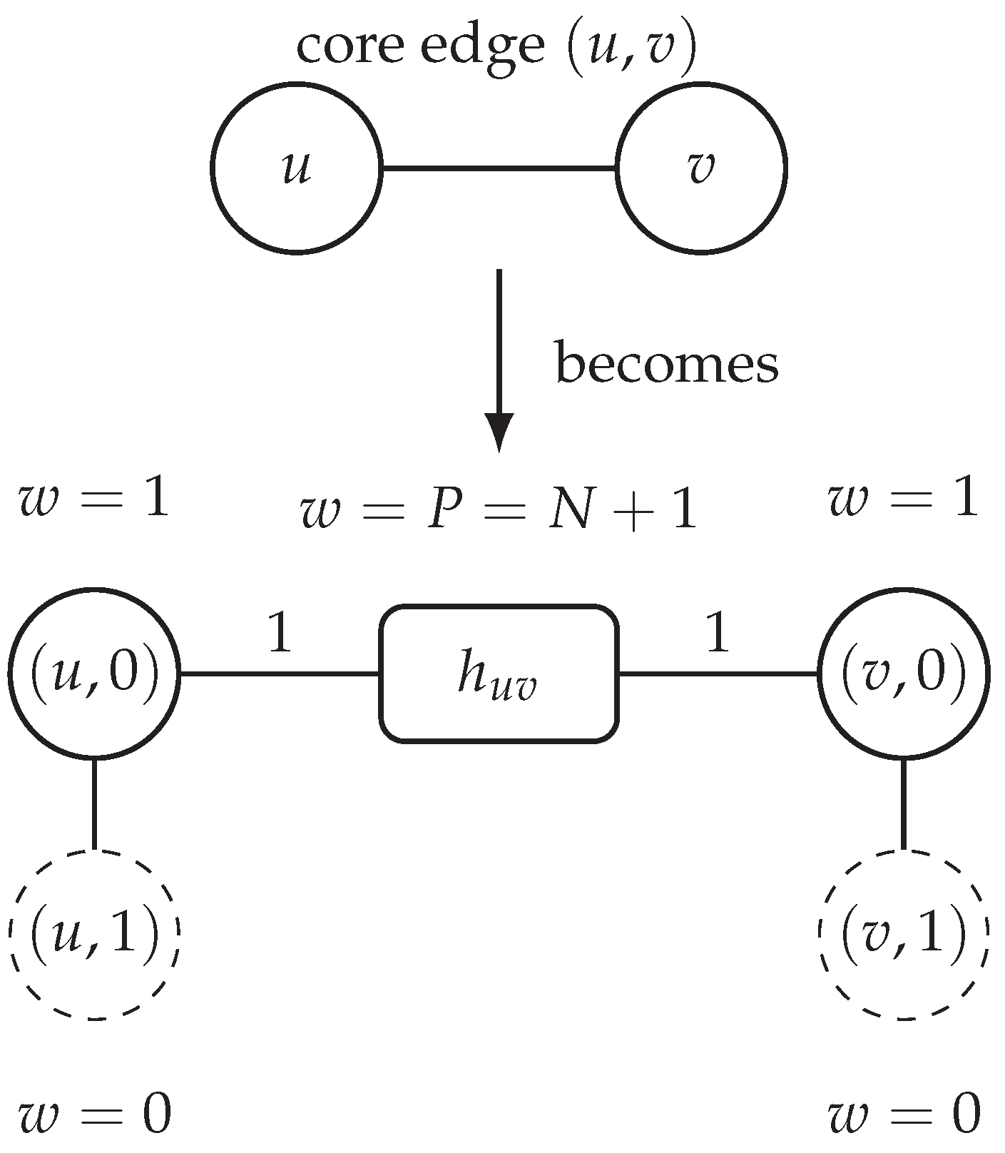

Table 1.
Code metadata for the Salvador package (v0.0.6).
| Nr. | Code metadata description | Metadata |
|---|---|---|
| C1 | Current code version | v0.0.6 |
| C2 | Permanent link to code repository | https://github.com/frankvegadelgado/salvador |
| C3 | Permanent link to reproducible capsule | https://pypi.org/project/salvador/ |
| C4 | Legal Code License | MIT License |
| C5 | Code versioning system used | git |
| C6 | Languages, tools, and services used | Python ≥ 3.12, NetworkX ≥ 3.4.2, NumPy ≥ 2.2.1, SciPy ≥ 1.15.0 |
| C7 | Compilation requirements and dependencies | Python, NetworkX, NumPy, SciPy |
Table 2.
Behaviour of FindVertexCover at the default across graph classes, from the car/ experiment (exact optima, no MILP; Konig certificates on bipartite instances). The worst case found anywhere attains the conjectured ceiling ; no instance exceeds it.
Table 2.
Behaviour of FindVertexCover at the default across graph classes, from the car/ experiment (exact optima, no MILP; Konig certificates on bipartite instances). The worst case found anywhere attains the conjectured ceiling ; no instance exceeds it.
| Graph class | Why the core solve (plus repair and pruning) tracks the optimum | Ratio |
|---|---|---|
| Stars | core optimum is the centre alone; decoded exactly | 1 |
| Matchings | core optimum is one endpoint per edge | 1 |
| Paths, trees, caterpillars | gadget reproduces the tree optimum exactly | 1 |
| Cycles | spanning-path gadget is a tree; solved optimally | 1 |
| Complete graphs | spanning-tree core solved; dense edges absorbed | 1 |
| Wheels / barbell / lollipop | optima on hub or clique vertices captured by the core | 1 |
| Chordal / interval | covers concentrate on simplicial hubs | |
| Random general () | near-optimal core plus small repair | |
| Grids / planar / outerplanar | core captures most edges; repairs only | |
| Graph atlas, | exhaustive small graphs | |
| Random bipartite (König) | non-core edges can survive the default layering | |
| Relabel/order stress of 7-vertex obstruction | ordering-dependent overshoot | |
| Bipartite hill-climb witness () | default layering overshoots on repair | (extremal) |
Table 3.
The car/ experiment for Salvador v0.0.6 under the default call . Ratios are with computed exactly without MILP (Konig certificates on bipartite instances). All covers are valid; the maximum ratio is , attained but not exceeded.
Table 3.
The car/ experiment for Salvador v0.0.6 under the default call . Ratios are with computed exactly without MILP (Konig certificates on bipartite instances). All covers are valid; the maximum ratio is , attained but not exceeded.
| Test class | Instances | Max ratio |
|---|---|---|
| Bipartite obstruction, canonical (exact) | 1 | 1.0000 |
| Relabel / order stress (exact) | 56 | 1.6667 |
| Random bipartite (exact) | 99 | 1.5000 |
| Bipartite hill-climb (exact) | 80 | 1.7500 |
| Grids, bipartite (exact) | 64 | 1.3333 |
| Graph atlas, | 1,245 | 1.3333 |
| Random general (exact, ) | 173 | 1.2500 |
| Total | 1,718 | 1.7500 |
Disclaimer/Publisher’s Note: The statements, opinions and data contained in all publications are solely those of the individual author(s) and contributor(s) and not of MDPI and/or the editor(s). MDPI and/or the editor(s) disclaim responsibility for any injury to people or property resulting from any ideas, methods, instructions or products referred to in the content. |
© 2026 by the author. Licensee MDPI, Basel, Switzerland. This article is an open access article distributed under the terms and conditions of the Creative Commons Attribution (CC BY) license.
Copyright: This open access article is published under a Creative Commons CC BY 4.0 license, which permit the free download, distribution, and reuse, provided that the author and preprint are cited in any reuse.


