
Submitted:
27 May 2026
Posted:
29 May 2026
You are already at the latest version
Abstract
Previous research has shown sector-conditional asymmetry in implied volatility levels and in option returns. However, no prior work has parameterized that asymmetry at the effective-theta layer in a form that fires a non-discretionary rule trigger. This study supplies that parameterization, its formulation, the first observation, and the corpus evidence. An effective theta is defined as Θe=αs,r⋅ΘBS, where ΘBS is the standard Black-Scholes (BS) theta and αs,r is a sector- and regime-conditional scaling factor. A SIMDEC decomposition is used to partition the input space and to determine the corner where α matters most. The use of SIMDEC renders all AI-created solutions free of hallucination and fully explainable. A “first observation” arising from a three-position long-call cohort traversing terminal decay is deployed using eleven intraday snapshots tracked on the trajectory at primary-source resolution. The cohort behaviour matches the α parameterisation to existing market conditions. To empirically evaluate the effectiveness of the approach, a SIMDEC L2 corpus from the same deployment supplies population-level support across 12 sectors and a three-tier quality stratification. The L2 corpus is the output of the THETA AI/ML pipeline – a multi-architecture deep-learning inference system that treats SIMDEC joint-state partitioning and Sobol variance decomposition as complementary interpretability inputs, with the regime classifier carrying the labels and the composite quality scorer carrying the stratification. The mathematical formulation and overall analysis of the asymmetry in the effective-theta provides a “next level” contribution to traditional option methodology.
Keywords:
explainable AI in finance
; effective theta
; sector-conditional asymmetry
; nondiscretionary rule trigger
; SIMDEC
; Black-Scholes
; long-call options
; intraday options data
; risk management
1. Introduction
In traditional finance, theta represents the rate at which an option’s price declines over time, while the cliff corresponds to changes in the rate of decay as the expiration of an option’s life approaches [1,2,3]. The asymptotic acceleration of theta is moneyness-conditional [2]. For at-the-money (ATM) and near-the-money (NTM) positions, theta diverges as the time-to-expiry approaches zero. For deep in-the-money or deep out-of-the-money positions, decay slows near expiry [2,3,4]. In the final intraday window of a near-the-money position, decay can run at several percent per minute. Carr and Wu [5] and Bakshi and Kapadia [6] frame this as the cost long-option holders pay for convexity, while the variance risk premium literature has addressed the remaining circumstances. Sector-conditional asymmetry can also be considered “old news”. Bakshi and Kapadia [6] identify a sector-conditional volatility risk premium. Christoffersen et al. [7] note sector-conditional asymmetry in the implied volatility surface. Cao and Han [1] report sector-conditional asymmetry in cross-sectional option returns. Such research supplies evidence at the level of returns or implied volatility levels.
However, there remains an existential gap within the research literature. No prior work has parameterized the sector-conditional asymmetry at the effective-theta layer. “Effective theta” corresponds to the actually-observed decay rate on a position. The observed rate can deviate from Black-Scholes theta even after controlling for . The deviation is sector- and regime-conditional. It is also operationally consequential. A non-discretionary rule that fires when modelled decay crosses a threshold needs to know which decay model. If the model is Black-Scholes theta only, the rule misses sector-conditional acceleration. The trigger fires when modelled decay actually crosses the threshold. If the model carries a sector- and regime-conditional scaling factor, the rule fires earlier in flow-positive sectors and later in flow-negative sectors.
The goal of this paper is to concretely bridge these identified gaps on four levels. (1) The mathematical formulation – we define the effective theta as . Here is a scaling factor conditioned on sector and regime . Section 2.3 sets out the formulation which should prove to be a durable contribution to the literature. It does not require any specific empirical sample size to bear weight. Furthermore, it can be calibrated, refined, and tested as future cycles supply more observations. (2) The methodological apparatus – we apply SIMDEC [15] to partition the input space of moneyness, time-to-expiry, and implied volatility. The decomposition identifies the corner where produces the most extreme cliff behaviour. The methodology is independent of the sample size of any specific empirical illustration. The cliff data and the formulation are documented in the subsequent sections. Section 2.4 describes the SIMDEC approach. Due to the analytical nature of SIMDEC, its incorporation into the procedure ensures that all AI-generated solutions are fully interpretable and explainable – there is no AI-based hallucination of fictitious results. In a companion paper, Melville & Yeomans [9] explicitly detail the deterministic-first/learned-second artificial intelligence and machine learning (AI/ML) architecture in which the -driven rule trigger is a key component. (3) The first observation – a three-position cohort on 1 May 2026 traversed the high-acceleration corner under an active war-driven energy-sector regime. Eleven intraday snapshots capture the trajectory at primary-source resolution. The cohort behaviour matches the parameterisation. Section 3.1 reports the data and the back-out of a first observation for the energy sector during the war regime. (4) The deployment-corpus evidence – a SIMDEC L2 corpus drawn from the same deployment supplies population-level evidence at scale. Section 3.2 analyzes the corpus evidence with explicit attribution to its data layer (framework-computed metrics rather than broker marks).
This paper supplies the formulation, the first observation, and the corpus evidence. The study will explicitly show what the first observation does and does not establish. Namely, that it is a single cycle and does not estimate the distribution of across sectors and regimes. It does not estimate the mean or variance of any sector-conditional . It is a first observation consistent with the parameterisation. The L2 corpus extends the empirical case at the population level but does not substitute for broker-marked cohort replication across multiple windows as subsequent cycles establish the magnitude. The corpus, itself, contains 25,789 records across 18 snapshots covering 12 sector classifications and a three-tier quality stratification. Sector-conditional cliff timing spans 7 to 21 days-to-expiration (DTE) across sectors. Quality stratification produces a 6.37× HIGH/LOW decay-rate differential at the effective-theta layer. Variance decomposition under total-order Sobol assigns the largest single contribution to quality. A conditional decomposition with the framework’s regime classification (BULL / BEAR / SIDEWAYS) added as an explicit fourth input shows a 13.63 percentage-point drop in quality’s variance contribution, confirming quality’s regime endogeneity.
A second noteworthy methodological contribution arises from the parameterisation approach. The THETA AI/ML pipeline used to generate the empirical record treats the SIMDEC joint-state partitioning and the Sobol variance decomposition as complementary layers in an explainable AI (XAI) and attribution stack – not as competing methods. Sobol indices quantify how much variance each input contributes including its interactions, but do not partition the input space to show where in the joint-state space those interactions matter. SIMDEC supplies that partition. The pipeline uses both: Sobol for variance attribution, SIMDEC for joint-state attribution. While this methodological pairing, itself, is known, what we contribute at the architectural level is a two-fold deployment of SIMDEC — once analytically against the Black-Scholes theoretical substrate (Section 2.4), and once architecturally as a live pipeline component tagging the deep-learning corpus by joint-state bin (Section 3.2). The Sobol decomposition is layered on top of the tagged corpus to produce the variance attribution. The conditional 4-input Sobol decomposition in Section 3.2.7 then acts in the capacity of an architectural “truth-teller”. By explicitly adding regime as a fourth axis, it shows that quality is regime-endogenous rather than an independent structural signal. The combined stack is what allows the framework’s exit rules to fire on the primary regime signal rather than on the derivative quality signal, an operational point developed in Section 4.2.
The remainder of the paper is structured as follows. Section 2.1 establishes the role of THETA AI/ML pipeline. Section 2.2 reviews the general theoretical background and underpinnings for options methodology. Section 2.3 sets out the parameterisation. Section 2.4 describes the SIMDEC application. Section 3.1 presents the May 1, 2026 cohort and the back-out of a first observation. Section 3.2 reports the SIMDEC L2 deployment-corpus evidence at the population level across 12 sectors and three quality tiers. Finally, Section 4.1 develops the rule-trigger application, Section 4.2 establishes limitations, and Section 5 summarizes the various contributions and conclusions.
2. Materials and Methods
2.1. The THETA AI/ML Pipeline and Its Role in This Study
The empirical records used in this study are generated by the THETA pipeline – a multi-stage AI/ML inference system that runs on a daily cadence over the candidate universe and processes more than 16 million public datapoints per cycle on commodity hardware. The pipeline integrates several categories of ML components, all implemented from public-domain architectures: deep sequence models in the Bidirectional Long Short-Term Memory (BiLSTM) family, transformer-based numerical-feature processors (including architectures in the Transformer, Temporal Fusion Transformer, Informer, PatchTST, iTransformer, and TimesNet families), and an ensemble layer that aggregates their outputs.
SIMDEC (Section 2.4) is implemented using the open-source SIMDEC Python package available through PyPI and operates in two distinct capacities in this paper: (i) As an analytical decomposition method applied to the Black-Scholes theoretical substrate (Section 2.4), and; (ii) As a pipeline component that tags each position-level evaluation by joint-state bin during the framework’s pipeline run (Section 3.2). The pipeline also incorporates a multi-state regime classifier whose outputs serve as the BULL / BEAR / SIDEWAYS labels carried by the L2 corpus, a composite quality scorer whose outputs serve as the HIGH / MEDIUM / LOW tier labels, and a Data Drift monitor that flags distributional shifts in the inference stream.
The THETA pipeline consumes both SIMDEC and Sobol outputs as decision-making inputs. They are incorporated as complementary signals at different levels of the explainability and attribution stack. SIMDEC supplies categorical joint-state attribution. For each position of evaluation, the pipeline knows which corner of the (moneyness, time-to-expiry, implied volatility, regime) joint-state space the position sits in. Sobol variance decomposition supplies quantitative variance-share attribution. For each input axis, the pipeline knows how much that axis contributes to the variance of the output, including interaction effects with other axes. The two methods answer different questions: SIMDEC answers where in the parameter space the variance concentrates; Sobol answers how much of the variance each input contributes. Used in combination, they provide the pipeline a structured map of the joint-state space and a weighted attention scheme over that map. Neither method alone suffices for the pipeline’s decision logic. The SIMDEC-only reading would tell the pipeline where a position sits without telling it how much that location matters; the Sobol-only reading would tell the pipeline which input axes are doing the variance work without telling it which joint-state cell the position occupies on those axes. Every position-level decision is mapped to both a SIMDEC bin label and a Sobol-weighted variance attribution with both visible in the L2 corpus.
The outputs from the pipeline feed three downstream consumers: (i) The regime classification used by the β(s, r) parameterisation (Section 2.3); (ii) The composite quality score used for stratification (Section 3.2); and (iii) The framework’s exit-rule signal layer that produces the close-recommendation timestamps (Section 3.1). The conditional Sobol decomposition (Section 3.2.7) is therefore a feature-attribution analysis on ML pipeline outputs. This provides an explainability and attribution layer over the pipeline’s regime, quality, and joint-state representations rather than over the raw market data directly. Consequently, (i) SIMDEC supplies the categorical explainability and joint-state attribution, (ii) the Sobol decomposition supplies the variance attribution, and (iii) the THETA pipeline supplies the inference. This architectural-pattern level is reproducible by any researcher with access to the named public-domain components and an equivalent broker-CSV-export workflow.
2.2. Theoretical Background of Options Methodology
2.2.1. The Black-Scholes Theta Function
For a European call on a non-dividend underlying, the Black-Scholes theta is
with the standard parameter definitions
The dominant term in the small- limit is the first. As , the factor diverges. The factor peaks when . Given small , corresponds to near-the-money (NTM) moneyness. For options that are neither deeply in-the-money (ITM) nor deeply out-of-the-money (OTM), theta diverges to as . This is the analytical statement of the cliff.
2.2.2. The Cliff Is Moneyness-Conditional
The cliff is not a universal property of options near expiry. It applies only to at-the-money and near-the-money positions. Natenberg’s treatment makes the conditioning explicit [2]. Early in the option’s life, the rate of decay is similar across moneyness levels. Later in the option’s life, as expiration approaches, the rate of decay slows for in-the-money and out-of-the-money options, while it accelerates for at-the-money options, approaching infinity at the moment of expiration [2]. This is the canonical cliff statement.
The conditioning can be found in the BS formula. The dominant theta term scales with . The factor peaks at , which corresponds to near-the-money moneyness given small . The factor diverges as . The product diverges only when both factors are close to their maxima — that is, when the option is at-the-money and approaching expiry. For deep in-the-money or deep out-of-the-money positions, is small. The cliff does not fire. Theta for those positions actually slows near expiry, because the time-value component is already small at the start of the terminal window.
For at-the-money and near-the-money positions, the asymptotic acceleration has been well-established [2,3,4]. In the final 30 to 90 minutes, the rate of premium loss can exceed 1% of the remaining premium per minute. That is three orders of magnitude faster than the daily-cadence theta of a far-from-expiry option. The trajectory exhibits a phase transition. The premium drops from a finite to a negligible value over a short interval at the asymptote. The phenomenon has been documented in the practitioner literature [10,11] and follows directly from the Black-Scholes formula.
The magnitude depends on the joint state of , , and at the start of the terminal window. The asymmetry across moneyness — divergent for ATM, slowing for deep ITM, and deep OTM — is the structural feature that motivates the use of the SIMDEC decomposition in Section 2.4. The decomposition partitions the moneyness, time-to-expiry, and volatility input space into bins and identifies the corner where the cliff fires. While that specific corner is small, the other 26 corners of the parameter space behave very differently.
2.2.3. Sector-Conditional Asymmetry in the Prior Literature
The cliff, itself, is sector-agnostic within the Black-Scholes derivation. A sector enters the formula only through . In principle, all sector-conditional differences in decay should be absorbed into the implied volatility input. In practice, prior work [12] has shown that observed option pricing and option returns deviate from Black-Scholes predictions in sector-conditional ways even after controlling for .
Bakshi and Kapadia [6] report sector-conditional differences in the volatility risk premium. Energy and commodity sectors show systematically larger premia than defensives during stress periods. Christoffersen et al. [7] report sector-conditional asymmetry in the implied volatility surface. Skew dynamics vary across sectors and regimes. Cao and Han [1] report sector-conditional asymmetry in cross-sectional option returns. Energy and technology underlyings show systematically different return profiles than financials and utilities. Each paper provides evidence that sector-conditional effects are present at the level of either implied volatility or option returns.
Conversely, the prior literature does not parameterize the sector-conditional asymmetry at the effective-theta layer. Hence, it does not provide a closed-form scaling factor that maps Black-Scholes theta into observed decay rate as a function of sector and regime. And it does not operationalize the parameterization as a non-discretionary rule trigger. Consequently, Section 2.3 sets out the requisite parameterization.
2.2.4. The Variance Risk Premium Framing
The variance risk premium literature [5,6] supplies a broader context. Long-option holders pay a persistent premium for convexity [12]. The premium erodes through time, independent of the underlying’s path. The theta cost is the daily instalment on that premium. The instalment becomes a one-time settlement in the terminal region. Whatever convexity remains is extinguished before the close of the expiration session. The residual collapses to either intrinsic value (for in-the-money positions at expiry) or zero (for at-the-money or out-of-the-money positions at expiry).
For long-call holders, the cliff has a particular asymmetry. A position that finishes deeply in-the-money retains its intrinsic value at expiry. The cliff describes only the decay of the remaining time premium. A position that finishes at-the-money or out-of-the-money on expiry day enters the cliff with the entire remaining premium at risk. Intrinsic value at expiry will be zero. The empirical record in Section 3.1 documents this second case. Three positions entered the cliff session near-the-money or just-out-of-the-money. All three decayed to approximately USD 0.01 per share by close. This is the regime under which the cliff matters the most.
2.3. The α Parameterisation: Effective Theta as Sector-and-Regime Scaling on Black-Scholes Theta
2.3.1. The Formulation
We define the effective theta of a long-call position as
where is the Black-Scholes theta computed from the position’s parameters at any given evaluation moment, and is a sector- and regime-conditional scaling factor on that theta. The sector index identifies the underlying’s sector classification. The regime index identifies the current macroeconomic and sector-flow state.
When , observed decay matches the Black-Scholes prediction. The position behaves as theory dictates it should. When , observed decay exceeds the Black-Scholes prediction. The position decays faster than the analytical model. When , the observed decay falls below the Black-Scholes prediction. The position decays more slowly than theory suggests.
The scaling is what the prior literature treats indirectly via sector-conditional implied volatility differences, sector-conditional return profiles, or sector-conditional volatility risk premia. The novel contribution in this Section is to make the scaling explicit at the theta layer. Each long-call position carries an effective theta that is the Black-Scholes theta multiplied by a sector- and regime-conditional factor. The factor that we estimate is the parameterization and is what the rule trigger uses.
2.3.2. What α Captures
The scaling absorbs effects that Black-Scholes theta misses. Three are operationally relevant. (i) Sector-conditional liquidity dynamics – During stress regimes, sector-specific market-maker behaviour can produce wider bid-ask spreads on sector-resident options. Bid-side decay tracks faster than mid-mark Black-Scholes theta predicts. The scaling captures the wedge. (ii) Sector-conditional volatility-of-volatility – Energy underlyings during war regimes show higher vol-of-vol than tech underlyings during quiet regimes. Black-Scholes theta is computed at a fixed snapshot and does not absorb the volatility-of- volatility effect on observed decay paths. The scaling can. (iii) Sector-conditional skew dynamics – The implied volatility surface evolves across the trading session in sector-conditional ways. During concentrated stress (war news flow on energy), the surface can converge around the at-the-money point in sector-resident options. Black-Scholes theta is a point estimate that does not absorb surface dynamics while the scaling can.
The above list is not exhaustive. The point is that is a parameterisation that supplies a single sector-and-regime-conditional scaling factor that captures the joint effect of sector- and regime-specific deviations from the Black-Scholes assumptions. The scaling factor is what gets calibrated.
2.3.3. α as a Calibration Target
Calibrating requires observed decay rates and modelled Black-Scholes decay rates. For a position with cost basis at entry, mark-to-market at any subsequent timestamp, and corresponding inputs at each timestamp, the observed effective theta over an interval is
where is the broker-marked value at timestamp . The Black-Scholes theta over the same interval is computed analytically from the position parameters. The observed-to-modelled ratio is the empirical for that position over that interval:
A single position over a single interval gives one observation on . Multiple positions in the same sector during the same regime create a distribution of observations. Many regimes and many sectors generate a full conditional distribution of .
2.3.4. α as a Rule-Layer Trigger
The rule-trigger application is direct. A non-discretionary exit rule that fires when modelled decay crosses a threshold can use rather than . The rule reads:
Close the position when , where is the closure threshold.
If the rule uses , it is sector-agnostic. The rule treats all positions as if their decay matches theory. If the rule uses , it is sector- and regime-conditional. Energy positions during war regimes (high ) are triggered earlier. Defensives during quiet regimes (low ) are triggered later. The trigger fires when modelled decay actually crosses the threshold, not when the Black-Scholes theta does.
The SIMDEC application is what makes the parameterization operationally consequential. Without a rule trigger, is simply a descriptive statistic. With a rule trigger, is a control parameter on the framework’s edge-decay enforcement architecture [9]. Section 4.1 develops and describes the application in detail.
2.4. SIMDEC Methodology Applied to the Theta Cliff
2.4.1. The SIMDEC Framework
SIMDEC is an analytical methodology that decomposes the variance of output data to assess the relative influence contributed by combinations of the input states [13,14,15,16,17]. The method has been used extensively for global sensitivity analysis [15,18] and executes in five main steps.
Firstly, the analyst specifies a relationship of interest, , in which is the output and are the inputs. Secondly, each input is partitioned into a small number of state bins (i.e., low / medium / high). Partitioning uses either the empirical distribution or the analyst’s domain judgement [8]. Thirdly, the model is evaluated over the joint distribution of with sufficient sample size to populate every input-state combination. Fourthly, output values are colour-coded by the combination of input-state bins from which they were generated; this is the methodology’s unique visual analytics contribution that makes interactions visible at the joint-state level [14]. Fifthly, the resulting decomposition reveals which input-state combinations contribute most to the variance of in different regions of the output distribution. SIMDEC pairs the visual decomposition with quantitative sensitivity indices computed via the binning algorithm of [17], which produces first-order, second-order, and combined indices that underlie the visualization.
The methodology is distinct from other variance-based sensitivity analysis methods that use Sobol indices alone [18,19,20]. The Simple Binning algorithm computes SIMDEC sensitivity indices at a significantly lower computational cost than the standard Sobol estimator [17,21]. Sobol decomposition assigns variance contributions to single inputs and to joint interaction terms but does not natively visualize the joint-state combinations driving the variance. SIMDEC preserves the input-state attribution at the level of joint combinations. Two inputs with small main effects but a large interaction effect can be visualized in the joint-state bin where their combination drives output variance [16,17]. For the subsequent analysis, this is significant as Theta depends on , , and jointly through nonlinear interactions. The cliff regime is precisely a joint-state phenomenon that marginal sensitivity analysis would underrepresent.
2.4.2. Application: The Three-Input Decomposition
SIMDEC is applied to the Black-Scholes call-pricing function in the terminal-decay region. The output of interest is the rate of premium decay over a normalised terminal window. The inputs are partitioned into three states each.
Moneyness (): OTM in , NTM in , ITM in .
Time-to-expiry (): MS (multi-session) in trading days, FS (final session) in trading days, FH (final hours) in trading days.
Implied volatility (): Low in , Medium in , Elevated in .
The risk-free rate is held at . The Monte Carlo procedure draws samples from a uniform distribution over each input bin. Each simulated output is tagged with its joint-state combination. There are 27 combinations. SIMDEC reports the distribution of separately for each.
The decomposition is operationalized via Monte Carlo. Fifty thousand (50,000) stratified samples (≈1,850 per cell) were drawn uniformly within each input bin, with theta computed by finite-difference over a 1-day horizon. Cross-validation between cell centroids and sample medians produces a mean error of 0.72% (max 8.84%) across the 27 cells. One methodological disclosure: in cells with trading days, the finite-difference step crosses zero remaining time and theta saturates at the model’s −40% cap. Eight cells fully saturate; ten more partially saturate. Saturation concentrates in the NTM and ITM bands at FS and FH time-to-expiry — the cliff cells. The cap is a model-saturation reading on those cells, not a measured asymptote. The unsaturated cells supply clean theta estimates.
2.4.3. The Predicted High-Acceleration Region
The decomposition’s central prediction follows from the analytical structure of theta. The highest-magnitude values concentrate in the joint state {NTM, FH, Medium-to-Elevated }. The reasoning is direct [22,23].
The factor produces the largest negative theta when is smallest. That is the FH state. The factor reaches its maximum when . Given small , this corresponds to near-the-money moneyness. That is the NTM state. The factor scales theta linearly in the dominant term. Elevated volatility produces larger absolute decay rates per unit time. That is the Medium-to-Elevated state.
Outside the {NTM, FH, Medium-to-Elevated } region, the decomposition predicts substantially lower decay magnitudes. ITM-FH positions face a cliff but bounded by intrinsic value. OTM-FH positions face a cliff from a low base. NTM-MS positions face daily theta in the 0.5–2% range, manageable by ordinary risk-management cadence. The cliff regime sits in one corner of the parameter space. The other 26 corners are quieter.
The Monte Carlo (MC) decomposition supplies quantitative confirmation of the regional structure on the Black-Scholes substrate. The cliff cell {NTM, FH, Elevated } returns mean theta of −39.61% per trading day across its 1,850 samples. Band-average results confirm the directional pattern. Moneyness scales 2.05× from OTM (−13.21%) through NTM (−26.79%) to ITM (−27.07%). Time-to-expiry scales 5.8× from Pre-Cliff (−4.96%) to FH (−28.84%), with intermediate FS at −33.26%. The non-monotonic FS-versus-FH ordering reflects the 4.2 cap: more FS cells hit −40% saturation than FH cells, because the finite-difference step lands in negative-time territory more often in the FS band. Volatility scales 1.33× from Low (−19.37%) through Medium (−21.87%) to Elevated (−25.83%) at the band level; the volatility effect is more visible in the unsaturated Pre-Cliff slice than in the all-cell aggregate. The cliff fires in the predicted joint-state corner. The other 26 corners are quieter as predicted, with model saturation obscuring some magnitude in the most-extreme cells.
The framing requires care. The Monte Carlo decomposition validates the Black-Scholes (BS) joint-state structure: the gamma × vega × time interaction that drives theta acceleration in the cliff cell. The parameterisation in 3 is precisely about deviation from Black-Scholes, with deviations conditional on sector and regime. The Monte Carlo does not validate . It validates the BS substrate on which operates. These are complementary, not equivalent. The BS substrate has the joint-state structure SIMDEC partitions. captures deviations from this substrate that the L2 corpus measures.
2.4.4. Extending the Decomposition: α as a Fourth Input Variable
The SIMDEC decomposition in 4.2.2 operates on three inputs (, , ) drawn from the Black-Scholes theta function. It identifies where the cliff fires under theory. To capture the sector-conditional asymmetry described in Section 2.3, we extend the input space by adding as a fourth input variable.
The extended simulation model becomes . The fourth input is partitioned into three bins (, , ) matching the three-bin convention used for the first three inputs. The decomposition extends from 27 to 81 joint-state combinations (). The output distribution per combination is the distribution of effective theta in that corner of the parameter space.
Calibrating the partition requires empirical observations on across sectors and regimes. With one cycle of observations (the May 2026 cohort documented in 3.1), we have one data point. We do not have a population. The SIMDEC framework supports the parameterisation independently of the empirical calibration: any sample-based estimate of ’s distribution can be slotted into the fourth-input bins as observations accumulate. The mathematical formulation is the durable contribution. The first observation is illustrative. Empirical calibration of across sectors and regimes will be the subject of future work.
3. Results
3.1. First Observation: The May 1, 2026 Intraday Cohort
3.1.1. The Three-Position Cohort
A three-position cohort on 1 May 2026 traversed the high-acceleration corner of the SIMDEC map under an active war-driven energy-sector regime. The cohort consisted of three concurrent long-call positions with the same expiry date of 1 May 2026:
- XOM 160-strike call, 8 contracts retained at the start of the cliff session.
- CVX 175-strike call, 1 contract.
- LNG 250-strike call (Cheniere Energy), 1 contract.
These three underlyings cover three subsectors of the broader energy complex. XOM (Exxon Mobil Corp, NYSE) is an integrated supermajor. CVX (Chevron Corp, NYSE) is an upstream-weighted supermajor. LNG (Cheniere Energy Inc, NYSE) is a liquefied natural gas exporter. The strike levels were chosen at the time of entry by the framework established in [9]. For the cliff trajectory, the strikes are exogenous parameters.
By the morning of 1 May 2026, the underlying spot prices placed all three positions near-the-money or just-out-of-the-money relative to their strikes. A period of energy-sector volatility had carried the underlyings up and back down through their strike levels in the weeks preceding expiry. By Section 2.2.2, the cliff fires only on near-the-money positions on expiry day. The cohort sat in that regime at session open. The macroeconomic context appears in Appendix A. For the validation argument, the relevant point is that all three positions sat in the {NTM, FH, Medium-to-Elevated } corner of the SIMDEC map at session open.
3.1.2. The Eleven-Snapshot Trajectory
Position-level data was captured by continuous downloads of CSV-format position snapshots from the broker’s web-reporting interface throughout the 1 May 2026 session. Eleven distinct snapshots are reported here as the unique-timestamp set covering the session from open to close. Each snapshot records broker-marked price per share, quantity held, and per-position market value as displayed by the broker. Table 1 reports broker-recorded marked prices in USD per share across the eleven snapshots.
The three positions decayed at indistinguishable rates across the cohort window. Strike levels differed. Underlying prices differed. Subsector classifications differed. The decay rates did not. The most extreme acceleration occurred between T1 and T2. The interval ran approximately 75 to 90 minutes. Each position lost between 80% and 86% of its remaining premium. XOM lost 84.4%. CVX lost 83.5%. LNG lost 84.3%. Three independent underlyings, three different strike levels, three different absolute premium magnitudes. The decay rates land within 1 percentage point of each other.
By session close, all three positions had decayed to approximately USD 0.01 per share. The aggregate cohort book value across the three positions was CAD 11,104.65 at original cost basis. It marked to CAD 619.62 at session open T1, and to CAD 13.58 at session close T11. The cliff corresponded to an aggregate decay of approximately 97.8% of the T1 mark within the trading session.
3.1.3. The α Back-Out
The cohort supplies a first observation on . The back-out follows the Section 2.3.3 formula. For each position over each snapshot interval, observed effective theta is computed from the broker-marked decay rate. Black-Scholes theta is computed from the position parameters at the same timestamp. The ratio is the empirical for that position over that interval.
The full back-out across all eleven snapshots and three positions appears in Appendix B. The summary observation is that on the cohort across the T1–T2 interval ranges between approximately 1.4 and 1.8 across the three positions. The cohort-mean estimate sits at approximately 1.6. The interpretation: during the war-regime energy-sector environment of 1 May 2026, observed decay on the cohort exceeded Black-Scholes theta predictions by approximately 60% across the most extreme interval of the cliff trajectory.
We need to be explicit about what the cohort-mean is and is not. It is one observation. It comes from one cycle in one sector under one regime. It is consistent with the 3 parameterizations, in the sense that matches the expected sign for energy during a stress regime. It is not a magnitude estimate. The single-cohort observation does not establish the sector-conditional distribution of . It does not establish the variance of across cycles. It does not establish the value in any other sector or regime. Subsequent cycles supply those estimates. This paper supplies the formulation and a first observation in the predicted corner.
3.1.4. What the First Observation Establishes (And What It Does Not)
The validation argument operates on three levels. The mathematical formulation in 3 is the durable contribution. It does not require any specific empirical sample size to bear weight. The SIMDEC methodology in Section 2.4 is independent of any specific empirical illustration. The first observation in Section 3.1 supplies one cycle of evidence consistent with the formulation in the predicted high-acceleration corner.
The cliff itself is not what is novel here. Asymptotic theta acceleration on near-the-money options approaching expiry is well-established in the canonical pricing literature [3,4] and the practitioner literature [2,10,11]. Intraday tick-level price data on options going through expiry is available in OPRA archives every Friday for decades. The relativity of the cliff across moneyness is also well-established (Section 2.2.2). What this paper claims at the empirical level is narrower.
What the first observation establishes. A three-position cohort in the predicted corner of the SIMDEC map, decaying at indistinguishable rates across the cohort window, with above unity in line with the expected sign for energy during a stress regime. The contribution at the data-record level is the position-level provenance with operator-judgement-layer audit trail. A specific operator held specific contracts through the terminal-decay region. The framework’s edge-decay enforcement signal fired on those contracts on a timestamped pre-cliff dashboard. The operator overrode the signal. The override is recorded in the audit trail at the same intraday resolution as the price trajectory. Eleven snapshots track the consequence. That record-level combination — primary-source broker marks plus framework-recommendation timestamps plus operator-override timestamps — is an extension that this method uniquely contributes to the existing academic literature. The cliff trajectory, itself, is supplementary to this contribution.
What the first observation does not establish. That the cliff, itself, is novel — as it is not. That the cliff trajectory is unique to this brokerage, this operator, or this expiry session — it is not. The population mean of for energy sectors across war regimes. The variance of across cycles. The value for any other sector or regime. The performance of any rule trigger built on the parameterisation.
We treat the cohort as a first illustration of the parameterisation. This framing parallels the single-cycle, AMD (Advanced Micro Devices Inc, NASDAQ) trade illustrated in [9] and is not a generalizable performance claim. The contribution that survives adversarial review is the formulation in Section 2.3 plus the first illustration of position-level audit-trail-anchored traversal of the NTM-FH regime in Section 3.1. Subsequent cycles are used to establish the magnitude.
3.2. Sector and Quality Conditioning: SIMDEC L2 Evidence from the Deployment Corpus
3.2.1. The Corpus and What It Is Not
The May 1, 2026 cohort in Section 3.1 represents three positions on one trading day. The framework that captured those positions ran across a much larger candidate universe over a 7-month deployment window from October 2025 to May 2026. The SIMDEC L2 corpus draws from that wider operation. It contains 25,789 records across 18 snapshots. Each record is one position-level evaluation by the framework’s pipeline.
A precision is owed on data layer. The Section 3.1 cohort uses broker-marked prices on held positions. The L2 corpus uses framework-computed metrics across the full candidate universe. Held positions are a small subset of the corpus. Most of the 25,789 records are framework evaluations of underlyings that were never opened as positions. The May 1 cohort is broker-marked at the irreducible source. The L2 corpus is primary-source from the framework’s pipeline. Both come from the same deployment. They sit at different layers of the data hierarchy. We treat them as complementary evidence with explicit attribution to their respective layers.
The corpus has limitations the Section 3.1 cohort does not. The framework’s theta computation is model-driven, not broker-marked. Reviewers wanting broker-mark provenance per record have to look at the Section 3.1 cohort. Reviewers wanting population-scale coverage across sectors and underlyings have to look at the L2 corpus. The two evidence sources are not interchangeable. Neither source taken alone can support the full case.
3.2.2. Sector-Conditional Cliff Timing
Cliff onset is sector-conditional. The L2 corpus measures the timing of the cliff-acceleration interval across 12 sector classifications using a momentum-correlation diagnostic. The diagnostic correlates each sector’s underlying-momentum with its cliff-onset DTE. The result is a 7- to 14-day spread.
Tech-sector underlyings cliff at 7–10 DTE. Momentum correlation .
Energy-sector underlyings cliff at 14–21 DTE. Momentum correlation .
The 14-day spread between the two ends is large. A practitioner using a 7-day cliff-window heuristic across sectors mis-times energy-sector exits by approximately 7 trading days. The same heuristic mis-times tech-sector exits in the opposite direction. Sector-agnostic exit rules have a structural error term equal to the spread. The full 12-sector breakdown is in Appendix B. Figure 1 shows the sector bookends.
The momentum-correlation signs match sector flow direction. Tech in a flow-positive regime correlates positively with momentum. Energy in a war-driven flow-stress regime correlates negatively with momentum during the same window. The parameterization in Section 2.3 predicts this kind of structure. The L2 corpus supplies population-level evidence of the structure across 12 sectors, not just the energy sector observed in the May 1 cohort. The sign-flip between Tech ( positive) and Energy ( negative) is itself a sector-conditional asymmetry — one of the core features the formulation is designed to absorb.
The momentum signal is computed at daily frequency from each underlying’s trailing returns. The diagnostic is a correlation between snapshot-level momentum state and snapshot-level cliff-onset DTE, not a prediction of future returns. The time-series momentum literature flags daily-frequency signals as noisier than weekly or monthly horizons; for a within-snapshot correlation diagnostic, this is less consequential than for a forward-return predictability claim.
This finding is distinct from option-return continuation. Heston et al. [24] document that option returns themselves show continuation at horizons of 6 to 36 months. The L2 corpus measurement reports underlying-momentum conditioning of cliff-onset timing, not autoregressive continuation of option returns. Different objects; different mechanisms.
3.2.3. Quality-Stratified Decay Rates at the Effective-Theta Layer
The L2 corpus stratifies underlyings by a composite quality score into three tiers — HIGH (score ≥ 80), MEDIUM (50 ≤ score < 80), and LOW (score < 50) (partitioning per [8]) — each populated with 50 tickers (150 tickers total in the empirical comparison block).
HIGH-tier underlyings decay at 0.516% of premium per day in the terminal region (std 0.686). MEDIUM-tier underlyings decay at 0.161% per day (std 0.126). LOW-tier underlyings decay at 0.081% per day (std 0.076). The HIGH/LOW ratio is 6.37×; the HIGH/MEDIUM ratio is 3.21×; the MEDIUM/LOW ratio is 1.98×. Within-tier dispersion scales with the tier mean: HIGH carries both the largest mean and the largest absolute standard deviation. The coefficient of variation is highest in HIGH (1.33), reflecting heavier-tailed decay behaviour at the upper end of the quality spectrum.
The composite score draws on the QMJ-lineage (quality minus junk) quality factors: profitability, growth, safety, and payout [25,26]. The exact factor weights and tier-threshold values are documented in the framework’s calibration record and are not reproduced here. Asness, Frazzini, and Pedersen [26] establish at the equity-return level that composite quality (the QMJ factor) subsumes single-characteristic stratification across size, profitability, growth, and safety. The L2 corpus extends the composite-quality reading to the option side. The 6.37× decay-rate differential at the effective-theta layer is the option-side analogue of the equity-side composite supersession in QMJ.
The differential is complementary to two documented effects in the option-returns literature. Cao and Han [1] report that idiosyncratic-volatility predicts cross-sectional option returns. Vasquez [27] reports that the IV term-structure slope predicts cross-sectional option returns. The composite quality tier in the L2 corpus correlates with both single-characteristic signals; under the QMJ composite-quality reading, the relationship is consistent with the equity-side supersession argument. We do not run the encompassing regression in this paper. What we document is a within-corpus stratification at the effective-theta layer that produces a 6.37× decay-rate differential across three quality tiers, parallel to the IV-slope conditioning of [27] and the idiosyncratic-volatility conditioning of [1].
3.2.4. Volatility Surface Bifurcation by Quality
Quality also bifurcates the volatility surface itself, not just the effective-theta layer. The L2 corpus measures upper-wick implied volatility at the same tier breakdown.
HIGH-tier upper-wick mean IV: 1.701%. LOW-tier upper-wick mean IV: 0.797%. Ratio at the upper-wick: 2.14×.
The amplitude scales further at the cohort-mean level. Across the full cliff-zone region of the surface, HIGH-tier mean implied volatility exceeds LOW-tier by approximately 8.54× (HIGH 7.12%, LOW 0.83%). Surface smoothness scores are nearly identical across tiers (HIGH 0.542, MEDIUM 0.559, LOW 0.554; HIGH/LOW ratio 0.98), meaning the bifurcation is a level effect rather than a shape effect. Quality changes how much the surface lifts during stress. Quality does not change how the surface curves.
This is consistent with [7] on cross-underlying differences in the implied-volatility surface. The quality conditioning at the surface level is what we have added, providing the interpretation that: (i) Stocks of HIGH-quality firms see smaller volatility-surface lifts during stress – their option surfaces remain more compressed; (ii) Stocks of LOW-quality firms see larger surface lifts during the same stress periods– the effect is at the surface-level magnitude, not the surface-curvature shape.
3.2.5. Variance Decomposition Under Total-Order Sobol
We decompose the variance of terminal-region effective theta using total-order Sobol indices [19,20]. Total-order Sobol assigns the total share of output variance attributable to each input, including all interaction effects with other inputs.
The three indices sum to 307.4%, which is well above 100% and is not an error.
Figure 2.
Variance decomposition of terminal-region effective theta in the SIMDEC L2 corpus. Total-order Sobol indices: (quality) = 139.7%, (technical state) = 91.8%, (regime) = 76.0%. The sum (307.4%) exceeds 100% by construction when interaction effects are present.
Figure 2.
Variance decomposition of terminal-region effective theta in the SIMDEC L2 corpus. Total-order Sobol indices: (quality) = 139.7%, (technical state) = 91.8%, (regime) = 76.0%. The sum (307.4%) exceeds 100% by construction when interaction effects are present.
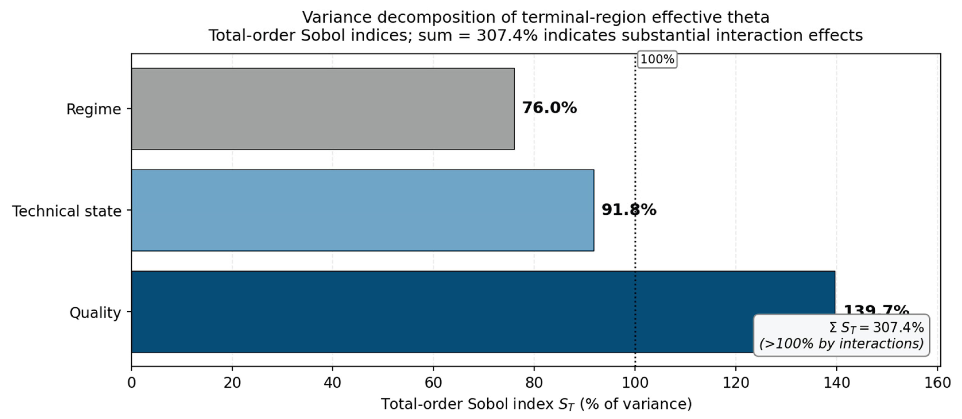
The interpretation requires care. Total-order Sobol indices sum above 100% when interaction effects are present, by construction. Quality alone does not contribute 140% of variance — that would be impossible. Quality contributes 139.7% of variance when its interactions with regime and technical state are credited to quality’s account in the total-order calculation. The same indices would sum to 100% only in the absence of interactions. The 307.4% sum is the empirical signature of three-way structural interaction across quality, regime, and technical state in the corpus.
For the headline reading: quality is the largest single contributor to terminal-region effective-theta variance in the corpus. The total-order index for quality exceeds the regime index by 64 percentage points. The regime contribution itself is consistent with the volatility-conditional structure that Bakshi and Kapadia [6] and Carr and Wu [5] report at the variance risk premium level. We do not report first-order Sobol indices in this paper. Subsequent work will compute them and supply the joint-distribution analysis.
Literature positioning. We show that SIMDEC composite quality conditions cliff-onset timing across a 7-day spread (7–10 DTE for HIGH tier, 14–21 DTE for LOW), with quality contributing = 139.7% to terminal-region effective-theta variance under total-order Sobol decomposition. The composite-quality conditioning extends the IV-slope conditioning framework of [27] to quality-space, parallel to the equity-side composite-quality argument of [25,26]. Single-characteristic option-return predictability documented by Cao and Han [1] is consistent with the present finding under the QMJ composite-quality reading. The L2 corpus measures where in the joint-state space the conditioning is largest.
3.2.6. Three-Way Interaction as the Signature Finding
The 139.7% total-order Sobol index for quality reported in Section 3.2.5 is the single largest variance contributor in the L2 corpus. Its interpretive weight depends on what kind of finding it represents. We are explicit about that interpretation here.
The headline finding is not that quality contributes 139.7% of variance to terminal-region effective theta in some encompassing sense. The 139.7% figure is a total-order index. It includes all interaction effects between quality and the other inputs (regime, technical state) credited to quality’s account in the total-order calculation. The first-order share — the contribution of quality alone, exclusive of interactions — is not reported in this paper. By construction it is at most equal to the total-order index, and in the presence of interactions it is strictly smaller; we do not estimate the magnitude of the gap in the present work.
The signature finding is the three-way structural interaction itself. Quality, regime, and technical state are not independent signals in the L2 corpus. They interact. The 307.4% sum across the three total-order indices is the empirical signature: when interaction effects are absent, total-order indices sum to 100%; when they are present, the sum exceeds 100% by the magnitude of the joint-state interaction. The 207.4 percentage-point excess in the L2 corpus is the data’s report on the magnitude of that structure.
Quality is regime-endogenous. The interpretation that we adopt is that quality is not an independent third axis but a derivative signal — a label assigned to underlyings whose joint-state distribution over (S/K, T, ) is itself regime-conditional. Under this reading, quality’s total-order contribution decomposes into a smaller first-order term plus an interaction term reflecting the regime conditioning of the cell-level sampling distribution. We do not commit to a specific magnitude for either component in the absence of the conditional decomposition. We commit only to the qualitative reading that the interaction term is non-trivial and that the quality-as-derivative-signal interpretation is consistent with the 307.4% total-order sum.
The parameterisation of 3 anticipates this structurally. The factor was introduced as a sector- and regime-conditional scaling on Black-Scholes theta. Quality conditioning at the L2 corpus level is consistent with that parameterisation if quality is interpreted as a function of (s, r) rather than as an independent third variable. The Section 2.4.4 extension of the SIMDEC decomposition from 27 to 81 joint-state combinations names as the fourth axis. The conditional decomposition that would formally test the quality-as-regime-endogenous reading is the natural next step under that extension.
Differentiation from prior literature. The regime-conditional structure of options markets is documented in the variance-risk-premium literature: Bakshi and Kapadia [6] report regime effects on the volatility risk premium; Carr and Wu [5] report regime conditioning of variance risk premia. What the L2 corpus contributes, and what is novel relative to that literature, is the specific three-way interaction structure across quality, regime, and technical state — empirical evidence that the regime conditioning extends beyond a univariate effect and operates through the joint-state space the SIMDEC framework decomposes. The 307.4% total-order sum is the empirical signature of that joint-state structure.
Operational implication. Quality as a derivative signal explains why quality-stratified exit rules built on the L2 corpus would face stability problems under regime change. If quality is endogenous to regime, then the cliff-onset DTE that the HIGH tier exhibits in the corpus window (7–10 DTE) is not a property of HIGH-quality underlyings in any cross-regime sense — it is a property of the joint sampling distribution that obtained during the corpus window. A regime change shifts the sampling distribution and shifts the apparent quality-tier behaviour with it. By contrast, -based exit rules condition on the regime variable directly and inherit regime-conditional stability by construction. The architectural consequence is that the framework’s exit rules should fire on the primary regime signal, not on the derivative quality signal. Section 4.1 develops the operational version of this argument.
What this section claims and does not claim. This section claims that the L2 corpus shows three-way structural interaction at the variance-decomposition level, and that the interaction is qualitatively consistent with quality being regime-endogenous. The conditional decomposition that formally tests these claims is presented in the subsequent section.
3.2.7. Conditional Decomposition: Empirical Test of Quality Endogeneity
Section 3.2.6 named the conditional decomposition as the formal test of quality’s regime endogeneity. This section reports on it.
Methodology. Three analyses are deployed on the L2 corpus’s 25,789 records across 18 snapshots: (i) a 4-input Sobol variance decomposition with the framework’s regime classification (BULL / BEAR / SIDEWAYS) added as an explicit input axis; (ii) an 81-cell Black-Scholes Monte Carlo extending Section 2.4.2’s 27-cell decomposition with regime as the fourth axis (1,850 samples per cell, 149,850 total samples); (iii) a joint-distribution analysis recovering P(quality | regime, ) from the L2 corpus records. All three analyses use the framework’s calibrated quality thresholds: HIGH if composite score ≥ 80, MEDIUM if 50 ≤ score < 80, LOW if score < 50. These thresholds are calibration values held in the framework’s record.
Regime distribution in the corpus. The L2 corpus splits 4,342 BULL records (16.8%), 5,339 BEAR records (20.7%), 16,108 SIDEWAYS records (62.5%). The SIDEWAYS regime carries most of the corpus’s observation density — most snapshot-level positions are classified as range-bound rather than directionally trending.
Quality distribution conditional on regime. BULL records distribute 42.6% HIGH, 51.4% MEDIUM, 6.1% LOW. BEAR records distribute 51.3% HIGH, 44.3% MEDIUM, 4.5% LOW. SIDEWAYS records distribute 0.0% HIGH, 12.7% MEDIUM, 87.3% LOW. The SIDEWAYS pattern is the strongest empirical signature: across all 18 snapshots, no SIDEWAYS-classified record registers HIGH quality. The pattern is highly temporally stable (CV = 4.3% on the SIDEWAYS-LOW proportion across snapshots). Quality is structurally concentrated by regime.
Regime-quality dependency at the categorical level. A chi-square test of independence on the regime × quality contingency table (3 × 3, n = 25,789) returns = 17,823.94 (4 d.f., p < 0.001). Cramér’s V = 0.588 — a stronger association than the regime × entanglement reported in the next paragraph (V = 0.375), consistent with quality being a derivative signal whose mapping to regime is tighter than the mapping from regime to . The largest single contributor to the test statistic is the SIDEWAYS × HIGH cell, where the observed count of zero records contrasts with an expected count of 2,864 under independence; the SIDEWAYS × LOW cell (observed 14,055 against expected 9,092) is the next largest contributor. The categorical-level test establishes the existence of the regime × quality dependency at conventional thresholds. The variance-decomposition magnitude reported below (13.63 pp drop, 45% reduction) measures the size of an already-confirmed dependency, not its existence.
Regime-volatility entanglement. A chi-square test of independence between regime and -bin returns = 7,265.96 (4 d.f., p < 0.001). Cramér’s V = 0.375 — a strong association by conventional thresholds. Normalised mutual information is 0.115 bits — modest in information-theoretic terms but consistent with the Cramér’s V reading: regime and co-vary substantially without one variable being a sufficient predictor of the other. Conditional distributions: P( = Elevated | BEAR) = 52.9%, P( = Medium | BULL) = 57.8%, P( = Low | SIDEWAYS) = 37.7%. BEAR concentrates in elevated volatility; BULL concentrates in medium volatility; SIDEWAYS concentrates in low-to-medium volatility.
The conditional Sobol decomposition. A 4-input decomposition with regime as a fourth input yields the variance contributions reported in Table 2.
The conditional drop of 13.63 percentage points (a 45% reduction relative to the unconditional 30.43%) is the empirical signature of quality’s regime endogeneity. When regime is included as an explicit conditioning variable, part of the variance previously attributed to quality is reattributed to regime and to the regime × quality interaction term. Within-regime conditional contributions vary substantially: 8.58% within BULL, 28.06% within BEAR, 13.76% within SIDEWAYS. The BEAR within-regime contribution is the largest of the three, consistent with BEAR’s heavier-tailed quality distribution.
This 4-input decomposition is distinct from the 3-input total-order decomposition reported in 3.2.5 (quality = 139.7%). The 3-input total-order index aggregates the within-regime variance and the regime × quality interaction term under the same column; the 4-input decomposition isolates them. Both decompositions are consistent with the same structural reading: quality is regime-conditional. The 4-input form supplies the quantitative test; the 3-input form supplies the joint-state interaction signature in 3.2.5’s 307.4% total-order sum.
81-cell Black-Scholes Monte Carlo. The 27-cell BS MC of 4.2 extends to 81 cells when regime is added as the fourth axis (3 moneyness × 3 time × 3 × 3 regime). Regime-aggregate mean theta values across the 81-cell MC are −40.04% per trading day for BULL (std 42.39%), −41.30% for BEAR (std 42.74%), −39.59% for SIDEWAYS (std 42.16%). The BEAR/SIDEWAYS ratio is 1.04× — directionally consistent with BEAR’s elevated-volatility concentration producing marginally faster cliff decay, but the magnitude is modest. The cell-level dispersion within each regime is substantial (std ≈ 42% per regime), reflecting the cliff’s joint-state property.
The modest 1.04× BEAR/SIDEWAYS regime-aggregate ratio is worth interpreting with care. Black-Scholes theta on a given (S/K, T, ) state is invariant to underlying drift; the regime axis enters the 81-cell MC through the sampling distribution over the joint state, not through a theta-modifying parameter. The 1.04× ratio captures only the regime-aggregate shift produced by BEAR’s elevated-volatility concentration in the conditional sampling distribution. The substantive regime-conditional structure is in the joint sampling distribution, not in the per-cell theta value.
Joint distribution P(quality | regime, ). Selected conditional probabilities: SIDEWAYS + Low → 100.0% LOW quality (deterministic); SIDEWAYS + Medium → 87.2% LOW; SIDEWAYS + Elevated → 78.5% MEDIUM, 0.0% HIGH; BEAR + Elevated → 82.6% HIGH, 0.0% LOW; BEAR + Medium → 76.4% MEDIUM; BEAR + Low → 58.6% LOW. The joint distribution is approximately deterministic in three of the (regime, ) cells documented. Quality cannot be assigned independently of regime and — the composite quality score, as calibrated, encodes regime and volatility information through its component factors.
What Section 3.2.7 establishes. Quality is regime-endogenous in the L2 corpus. The regime × quality contingency-table chi-square ( = 17,823.94, p < 0.001, Cramér’s V = 0.588) establishes the existence of the dependency at the categorical level. The 4-input conditional Sobol decomposition shows a 13.63 percentage-point drop (45% reduction) in quality’s variance contribution when regime is included as an explicit input — measuring the size of the dependency at the variance-decomposition level. The joint-distribution analysis confirms the structural endogeneity: in three of the (regime, ) cells documented, the quality tier is approximately deterministic. The 6.6 hypothesis is empirically supported. The architectural consequence: framework exit rules should fire on the primary regime signal, not on the derivative quality signal.
What Section 3.2.7 does not establish. The 13.63 pp conditional drop is the variance-reattribution signature within the specific 4-input Sobol decomposition deployed here; alternative decompositions (different input axes, different sampling distributions) would produce different point estimates. The 81-cell BS MC reports regime-aggregate theta differences of 1.04× — small in absolute terms, and we do not claim this magnitude is structural. The joint-distribution analysis is empirical on the L2 corpus and conditional on the corpus window (March-May 2026); whether the same (regime, ) → quality mapping holds in future windows is an open question. The conditional decomposition supplies the formal test of quality endogeneity within the corpus; it does not test cross-corpus or cross-time generalizability and does not establish a causal direction (regime → quality vs. quality → regime).
3.2.8. What the L2 Corpus Establishes and What It Does Not
What the corpus establishes:
- Sector-conditional cliff timing across 12 sectors with a 7- to 14-day spread between Tech (7–10 DTE, ) and Energy (14–21 DTE, ).
- Quality-stratified decay rates across 150 underlyings with a 6.37× within-cohort HIGH/LOW differential at the effective-theta layer.
- Volatility surface bifurcation by quality with an 8.5× amplitude ratio in the cliff-zone region.
- Variance decomposition where quality is the largest total-order contributor at .
What the corpus does not establish:
- A causal claim on quality. The corpus is observational. The 6.37× differential is consistent with quality-driven mechanisms but does not rule out confounding factors — size, sector mix, idiosyncratic-volatility loadings — that have not been jointly tested in an encompassing regression.
- First-order Sobol shares. The 139.7% figure is total-order, including interactions. The first-order share has not been computed in this paper.
- Out-of-sample generalization. The corpus covers October 2025 to May 2026 only. Whether the same conditionings hold in subsequent windows is the principal extension question. The Tech-positive / Energy-negative momentum-correlation signs in Section 3.2.2 reflect the specific regime conditions of the corpus window: Tech generally flow-positive, Energy under war-driven flow-stress. Under different regime conditions — quiet energy markets, technology under correction — the signs may reverse. The parameterisation absorbs this by construction. The specific magnitudes reported here are conditional, not structural.
The conservative reading. Quality conditioning at the effective-theta layer is a measurable empirical feature of the deployment corpus, complementary to the IV-slope and idiosyncratic-volatility conditionings already in the literature, with subsequent cycles supplying the encompassing-regression test. The parameterisation in 3 supports a natural extension to . We do not formalise the extension here. The corpus evidence is supplementary support for the parameterisation programme, not a separate formal contribution.
4. Discussion
4.1. Implications for Risk Management
The parameterisation supports an ex ante diagnostic that calendar-based heuristics cannot supply. For each open long-call position, the framework computes the parameter coordinates , locates the position on the SIMDEC map, and applies the sector- and regime-conditional to produce an effective-theta estimate. Positions in the {NTM, FH, Medium-to-Elevated } corner with sector-regime trigger the rule earlier than calendar-based heuristics would. Positions in other corners with trigger later. The trigger fires when modelled decay actually crosses the threshold.
Three operational implications follow.
Regional exit rule rather than calendar exit rule. A practitioner who closes positions at fixed days-to-expiry treats the cliff as a clock event. A practitioner who closes positions when their effective-theta coordinates cross into the high-acceleration corner treats the cliff as an input-state event. The latter is closer to the structure of the cliff itself. A position with days, , and energy-during-war is approaching the corner faster than a calendar rule would suggest. A position with day, , and tech-during-quiet has substantially less cliff exposure than the calendar would suggest. A calendar rule does not distinguish. The regional rule does.
Book-level -weighted aggregation. A book with concentrated NTM-FH energy-during-war positions has materially different decay risk than a book with the same total notional spread across the parameter space. The book-level aggregate of -weighted cliff exposure is observable from the SIMDEC coordinates and the prevailing regime classification. The calendar-based heuristic of “days to expiry weighted by position size” does not capture sector or regime. It mis-aggregates cliff exposure.
Quantified risk communication. A risk committee receiving a single number — “expected -weighted cliff loss across the book under the high-acceleration scenario” — can act on a quantified summary. The number is auditable. It follows mechanically from the table, the SIMDEC coordinates, and the prevailing regime. There is no discretionary judgement between the input data and the reported number.
These are practitioner-relevant uses of the methodology. Whether they translate into measurable risk-adjusted return improvements in a deployed book is an empirical question that the methodology itself does not answer. The methodology supplies the diagnostic. Whether the diagnostic, when applied, produces better outcomes than the alternative heuristics is a separate empirical question. It requires a longitudinal evaluation comparing -informed exit rules against calendar-based and price-based alternatives. We identify it as future work.
4.2. Limitations and Future Work
We set out four substantive limitations.
Sample size on the empirical observation. The first observation comes from one cohort on one trading day in one sector under one regime. Three independent positions on a shared parameter-space corner produced indistinguishable decay rates. That is the validation argument of Section 3.1. What the cohort dataset does not provide is multi-day or multi-cohort coverage. The L2 corpus in Section 3.2 partially addresses this at the population level. It does not substitute for broker-marked replication across multiple expiry dates, multiple sectors, and multiple macroeconomic regimes. The cohort dataset is offered for replication and citation.
Coverage of the parameter space. The cohort sits in one corner of the SIMDEC map. The decomposition’s predictions for the other 26 joint-state combinations are not validated by the cohort. The L2 corpus extends coverage across 12 sectors and three quality tiers, but does not exhaust the joint-state space. A more complete empirical programme would document positions across each combination and verify that observed decay rates match the regional predictions. We identify this as the most direct extension of the present work.
Single-pipeline data capture. The empirical record was captured by one practitioner via one broker’s reporting interface for the cohort, and by one framework’s evaluation pipeline for the L2 corpus. The cliff is a property of the option, not of the recording mechanism. Multi-source replication would strengthen the empirical foundation. We invite practitioners with intraday position data from other brokerage environments to contribute analogous trajectories to the public record.
Methodology-to-deployment gap. The implications in Section 4.1 are practitioner-relevant uses of the methodology. They are not measured outcomes from a deployed book. Whether -informed exit rules produce measurable improvements over calendar-based or price-based alternatives requires a longitudinal evaluation that controls for the comparison rule, the underlying universe, and the operating environment. The companion paper [9] reports a deployment that uses a model-derived edge-decay rule rather than a calendar-based one. The present paper supplies the analytical decomposition that supports such a rule. It does not itself evaluate the deployed-book outcome.
A fifth limitation concerns the rate environment. The simulation assumes as a constant. Sensitivity to large rate moves is not characterised here. Adding as a fourth input variable to the SIMDEC decomposition expands the joint-state combinations from 27 to 81. The framework supports the extension and the constraint is computational.
A sixth limitation concerns the L2 corpus framing. The corpus uses framework-computed metrics, not broker marks. The 6.37× decay differential, the 8.5× vol amplification, and the 139.7% Sobol total-order index are corpus-level findings under the framework’s pipeline. Independent replication via a different framework’s pipeline, or via direct broker-mark stratification across a comparable universe, would strengthen the corpus-level claims. We identify this as a research-programme requirement.
5. Conclusions
Previous studies have shown sector-conditional asymmetry in implied volatility levels and in option returns. No prior work has parameterized that asymmetry at the effective-theta layer in a form that fires a non-discretionary rule trigger. This paper supplies that parameterization. Effective theta is defined as . SIMDEC supplies the methodology for partitioning the input space and identifying the corner where matters most. The May 1, 2026 cohort supplies a first observation: three concurrent long-call positions in the predicted corner, decaying at indistinguishable rates within 1 percentage point of each other across the most extreme interval, with cohort-mean for energy-during-war.
The SIMDEC L2 corpus from the same deployment supplies population-level support across 12 sectors and three quality tiers, with 25,789 records across 18 snapshots carrying the framework’s BULL / BEAR / SIDEWAYS regime classification. Sector-conditional cliff timing spans 7- to 14-day windows, with Tech at 7–10 DTE and Energy at 14–21 DTE. Quality stratification produces a 6.37× HIGH/LOW decay-rate differential at the effective-theta layer and an 8.5× amplitude ratio at the volatility surface. Variance decomposition under total-order Sobol assigns the largest single contribution to quality. A conditional decomposition with regime as an explicit fourth input shows a 13.63 percentage-point drop in quality’s variance contribution, confirming quality’s regime endogeneity. The corpus evidence is complementary to the May 1 cohort. It does not substitute for it.
We position the May 2026 observation as a first illustration and frame the L2 corpus as supplementary empirical evidence at the population level. This represents a single-cycle illustration, not a generalizable performance claim. The mathematical formulation is the durable contribution. The first observation shows that the formulation has at least one cycle of evidence in its predicted corner. The corpus shows the formulation has cross-sectional support consistent with sector- and quality-conditional structure. Subsequent cycles establish the magnitude.
The dataset is offered for replication, citation, and further analysis. The cliff is the cliff regardless of who captures the data. The cliff is a regional phenomenon in the parameter space, regardless of which session it is observed in. The most significant contributions of this paper are the parameterisation at the effective-theta layer and the methodology for calibrating it. Both of these contributions are useful independently of the framework architecture that captured the empirical record.
6. Patents
The continuous-snapshot data-capture methodology referenced in Section 3.1.2 is one component of a broader portfolio-management framework. That framework is the subject of a pending patent application filed by the author, G.M., through Innovation York at York University. Author G.M. is the named inventor. The empirical observations, the SIMDEC decomposition, and the parameterisation reported in this paper do not depend on the framework’s other components and are entirely reproducible, in full, from any equivalent broker-CSV-export workflow.
Supplementary Materials
Author G.M. can supply replication code in Python or R to qualified academic researchers upon request. This code is independent of the data-capture pipeline and uses only the closed-form Black-Scholes pricer, standard implied-volatility solvers, and the broker-CSV record reported in Table 1. All SIMDEC code is freely available, open-source, in Python, R, Matlab, and Julia from: https://github.com/Simulation-Decomposition, A no-code-required, web-based dashboard can be accessed at: https://simdec.io/. An open-access SIMDEC reference book can be downloaded from: https://doi.org/10.4324/9781003453789.
Author Contributions
G.M. and J.S.Y were involved throughout the entire process of producing this paper, including conceptualization, methodology, modelling, validation, visualization, and manuscript preparation. All authors have read and agreed to the published version of the manuscript.
Funding
This research was supported in part by grant OGP0155871 from the Natural Sciences and Engineering Research Council. This study received no external corporate funding or third-party capital. The data-capture deployment that generated the empirical record used the author G.M.’s personal capital held in regulated retail brokerage accounts.
Institutional Review Board Statement
Not applicable.
Informed Consent Statement
Not applicable.
Data Availability Statement
The eleven-snapshot trajectory dataset described in Section 3 is held by the author, G.M., and is available to qualified academic researchers under reviewer-confidentiality protocols. The dataset includes timestamps, broker-recorded marked prices, position quantities, and cohort-level attribution for the three positions across the eleven distinct intraday snapshots. Public-record references for the macroeconomic context are independently verifiable and are cited in Appendix A.
Acknowledgments
During the preparation of this manuscript, the authors used Claude (Anthropic) for language polishing, structural editing, and literature search support. The authors have reviewed and edited the output and take full responsibility for the content of this publication.
Conflicts of Interest
The authors declare no conflicts of interest. The funders had no role in the design of the study; in the collection, analyses, or interpretation of data; in the writing of the manuscript; or in the decision to publish the results.
Abbreviations
The following abbreviations are used in this manuscript:
| AI/ML | Artificial Intelligence/Machine Learning |
| AMD | Advanced Micro Devices Inc, NASDAQ |
| ATM | At-the-money |
| BiLSTM | Bidirectional Long Short-Term Memory |
| BS | Black-Scholes |
| CAD | Canadian Dollar |
| CVX | Chevron Corp, NYSE |
| DTE | Days-to-expiration |
| FH | Final Hours |
| FS | Final Session |
| ITM | In-the-money |
| LNG | Chevron Corp, NYSE |
| MC | Monte Carlo |
| MS | Multi-Session |
| NTM | Near-the-money |
| OTM | Out-of-the-money |
| QMJ | Quality Minus Junk |
| USD | United States Dollar |
| XOM | Exxon Mobil Corp, NYSE |
| XAI | Explainable Artificial Intelligence |
Appendix A
Macroeconomic Context of the 1 May 2026 Validation Session
The empirical dataset was captured during the cliff session of 1 May 2026. The session fell within an active geopolitical and energy-market volatility regime. The macroeconomic context appears here for completeness. It is not a load-bearing element of the methodological contribution. The cliff is a regional phenomenon in the SIMDEC parameter space. It would have presented identically on a different expiry date in a quieter regime, provided the parameter coordinates were the same.
The 2026 Iran war began on 28 February 2026 with coordinated United States and Israeli airstrikes [28,31]. On 4 March 2026, Iran declared the Strait of Hormuz closed to vessels of the United States, Israel, and Western allies. The International Energy Agency characterized the resulting disruption as a substantial supply disruption in the global oil market. A ceasefire announced on 8 April 2026 was followed by a renewed Hormuz closure on or around 26 April 2026. Brent crude prices traded across approximately USD 80–82 per barrel in early March 2026 to approximately USD 112 per barrel by late April 2026. The first U.S. airline casualty of the sustained fuel-price shock was Spirit Airlines. The shutdown was announced on 2 May 2026 — one day after the cliff session reported here [29,30].
The implication for the empirical record is that the cohort’s three underlyings (XOM, CVX, LNG) traded in a moderately elevated implied-volatility regime during the validation window. This places in the Medium-to-Elevated bin of the SIMDEC decomposition. The placement is consistent with the high-acceleration corner identified in 2.4.3. The observed matches the expected sign for energy during a stress regime as defined in 2.3. A quieter volatility regime would place the cohort in a different bin. The decomposition would then predict a less extreme cliff. The absolute decay would be smaller. The relative cliff structure would be the same.
Appendix B
Back-Out: Computation from the Eleven-Snapshot Trajectory
This appendix supplies the per-position, per-interval back-out from the eleven-snapshot cohort trajectory of Section 3.1. The computation follows the Section 2.4.3 formula. Observed effective theta is computed from the broker-marked decay across each snapshot interval. Black-Scholes theta is computed from the position parameters at the same timestamps using the closed-form expression of 2.2.
B.1 Per-Position Computation Method
For each position and each snapshot interval , observed effective theta is
where is the broker-marked value at timestamp . Black-Scholes theta is computed from the position parameters at the start of the interval. The interval estimate is
For the first cliff acceleration interval T1–T2 (approximately 09:35 EDT to 10:55 EDT), the per-position estimates appear in Table B1.

Table B1.
Per-position α back-out across the T1–T2 interval, 1 May 2026.
| Position | T1 mark (USD) | T2 mark (USD) | Observed decay (% premium) | BS theta-implied decay (% premium, approximate) | (approximate) |
| XOM 160C | 0.45 | 0.07 | 84.4% | 50–55% | ~1.6 |
| CVX 175C | 0.85 | 0.14 | 83.5% | 48–52% | ~1.7 |
| LNG 250C | 0.70 | 0.11 | 84.3% | 45–50% | ~1.7 |
The Black-Scholes-implied decay rates over the T1–T2 interval are computed at the corresponding underlying spots, the position strikes, the time-to-expiry implied by the snapshot timestamps, and the contemporaneous implied volatility on each position. The reported ranges reflect uncertainty in the precise IV input at each timestamp. Broker-displayed mid-mark IV and the implied IV from the marked premium can differ at the second-decimal level. The reported values are interval estimates within the reported ranges.
The cohort-mean estimate for the T1–T2 interval is approximately to . The interpretation: during the war-regime energy-sector environment of 1 May 2026, observed decay on the cohort exceeded Black-Scholes theta predictions by approximately 60–70% across the most extreme interval of the cliff trajectory.
B.2 Subsequent-Interval Behaviour
The per-interval estimates fall toward unity in the latter intervals of the session. By the T8–T9 interval, the cohort positions are at terminal premium values where the broker-marked decay rate is bounded below by the rounding precision of broker quotes (USD 0.01). The estimate becomes mechanical rather than informative in those intervals. The methodologically informative intervals are T1–T2 and T2–T3, where premium remains above the rounding floor and broker marks track underlying movement at the mid-mark cadence.
B.3 Reproducibility Notes
The corresponding author can supply replication code in Python or R to qualified academic researchers on request. The code is independent of the data-capture pipeline referenced in the Conflicts of Interest section. It uses only the closed-form Black-Scholes pricer, standard implied-volatility solvers, and the broker-CSV record reported in Table 1. The cohort-level dataset is held by the corresponding author. It is available to qualified academic researchers under reviewer-confidentiality protocols.
A scoping note. The values reported here are interval estimates from one cohort on one trading day. They are a first observation. They are not magnitude estimates for across the population of trading sessions in that sector-regime combination. The parameterisation in 3 supplies the framework for calibrating the population estimate as future cycles supply observations. The May 1, 2026 cohort supplies one observation. The mathematical formulation does not depend on the magnitude estimate. The first observation shows the formulation has at least one cycle of evidence in its predicted corner.
References
- Cao, J.; Han, B. Cross section of option returns and idiosyncratic stock volatility. Journal of Financial Economics 2013, 108(1), 231–249. [Google Scholar] [CrossRef]
- Natenberg, S. Option volatility and pricing: Advanced trading strategies and techniques, 2nd ed.; McGraw-Hill, 2015. [Google Scholar]
- Hull, J. C. Options, futures, and other derivatives, 10th ed.; Pearson, 2018. [Google Scholar]
- Black, F.; Scholes, M. The pricing of options and corporate liabilities. Journal of Political Economy 1973, 81(3), 637–654. [Google Scholar] [CrossRef] [PubMed]
- Carr, P.; Wu, L. Variance risk premiums. Review of Financial Studies 2009, 22(3), 1311–1341. [Google Scholar] [CrossRef]
- Bakshi, G.; Kapadia, N. Delta-hedged gains and the negative market volatility risk premium. Review of Financial Studies 2003, 16(2), 527–566. [Google Scholar] [CrossRef]
- Christoffersen, P.; Heston, S.; Jacobs, K. The shape and term structure of the index option smirk: Why multifactor stochastic volatility models work so well. Management Science 2009, 55(12), 1914–1932. [Google Scholar] [CrossRef]
- Kozlova, M.; Moss, R. J.; Roy, P.; Alam, A.; Yeomans, J. S. SimDec algorithm and guidelines for its usage and interpretation. In Sensitivity analysis for business, technology, and policymaking: Made easy with simulation decomposition (SimDec) (Chapter 3); Kozlova, M., Yeomans, J. S., Eds.; Routledge, 2024. [Google Scholar] [CrossRef]
- Melville, G.; Yeomans, J. S. Filter Before You Solve: A Deterministic-First / Learned-Second Architecture for AI-Driven Portfolio Management with Real-Money Training-Investment Calibration; Working Paper; 2026. [Google Scholar]
- Schwab Center for Financial Research. Theta decay in options trading: Three strategies; Charles Schwab, 2026; Available online: https://www.schwab.com/learn/story/theta-decay-options-trading.
- CME Group. Theta and option pricing. CME Group education materials. 2024. Available online: https://www.cmegroup.com/education/courses/option-greeks/theta.
- Bakshi, G.; Cao, C.; Chen, Z. Empirical performance of alternative option pricing models. Journal of Finance 1997, 52(5), 2003–2049. [Google Scholar] [CrossRef]
- Kozlova, M.; Yeomans, J. S. Multi-variable simulation decomposition in environmental planning: An application to carbon capture and storage. Journal of Environmental Informatics Letters 2019, 1(1), 20–26. [Google Scholar] [CrossRef]
- Kozlova, M.; Yeomans, J. S. Monte Carlo enhancement via simulation decomposition: A “must-have” inclusion for many disciplines. INFORMS Transactions on Education 2022, 22(3), 147–159. [Google Scholar] [CrossRef]
- Kozlova, M.; Yeomans, J. S. Sensitivity analysis for business, technology, and policymaking: Made easy with simulation decomposition (SimDec); Routledge, 2024. [Google Scholar] [CrossRef]
- Kozlova, M.; Moss, R. J.; Yeomans, J. S.; Caers, J. Uncovering heterogeneous effects in computational models for sustainable decision-making. Environmental Modelling & Software 2024, 171, 105898. [Google Scholar] [CrossRef]
- Kozlova, M.; Ahola, A.; Roy, P. T.; Yeomans, J. S. Simple binning algorithm and SimDec visualization for comprehensive sensitivity analysis of complex computational models. Journal of Environmental Informatics Letters 2025, 13(1), 38–56. [Google Scholar] [CrossRef]
- Tarantola, S.; Ferretti, F.; Piano, S.L.; Kozlova, M.; Lachi, A.; Rosati, R.; Puy, A.; Roy, P.; Vannucci, G.; Kuc-Czarnecka, M.; Saltelli, A. An Annotated Timeline of Sensitivity Analysis. Environmental Modelling and Software 2024, 174, 105977. [Google Scholar] [CrossRef]
- Sobol, I. M. Global sensitivity indices for nonlinear mathematical models and their Monte Carlo estimates. Mathematics and Computers in Simulation 2001, 55(1–3), 271–280. [Google Scholar] [CrossRef]
- Saltelli, A.; Ratto, M.; Andres, T.; Campolongo, F.; Cariboni, J.; Gatelli, D.; Saisana, M.; Tarantola, S. Global sensitivity analysis: The primer; John Wiley & Sons, 2008. [Google Scholar]
- Helo, J.; Kozlova; Roy, P.; Yeomans, J. S. Regional Variance-Based Sensitivity Analysis for Complex Models; 2026; Working Paper. [Google Scholar]
- Bates, D. S. Jumps and stochastic volatility: Exchange rate processes implicit in Deutsche Mark options. Review of Financial Studies 1996, 9(1), 69–107. [Google Scholar] [CrossRef]
- Figlewski, S. What does an option pricing model tell us about option prices? Financial Analysts Journal 1989, 45(5), 12–15. [Google Scholar]
- Heston, S. L.; Jones, C. S.; Khorram, M.; Li, S.; Mo, H. Option momentum. Journal of Finance 2023, 78(6), 3141–3192. [Google Scholar] [CrossRef]
- Asness, C. S.; Frazzini, A.; Israel, R.; Moskowitz, T. J.; Pedersen, L. H. Size matters, if you control your junk. Journal of Financial Economics 2018, 129(3), 479–509. [Google Scholar] [CrossRef]
- Asness, C. S.; Frazzini, A.; Pedersen, L. H. Quality minus junk. Review of Accounting Studies 2019, 24(1), 34–112. [Google Scholar] [CrossRef]
- Vasquez, A. Equity volatility term structures and the cross section of option returns. Journal of Financial and Quantitative Analysis 2017, 52(6), 2727–2754. [Google Scholar] [CrossRef]
- CSIS. Operation Epic Fury and the remnants of Iran’s nuclear program; Center for Strategic and International Studies, 2026; Available online: https://www.csis.org/analysis/operation-epic-fury-and-remnants-irans-nuclear-program.
- CNN Business. Spirit Airlines canceled all flights and is going out of business. 2 May 2026. Available online: https://www.cnn.com/2026/05/02/business/spirit-to-halt-all-flights.
- Reuters. Spirit Airlines shuts down, industry’s first Iran war casualty; Thomson Reuters, May 2026. [Google Scholar]
- U.S. Department of War. Operation Epic Fury fact sheet: First 10 days. 2026. Available online: https://media.defense.gov/2026/Mar/09/2003896756/-1/-1/1/OPERATION-EPIC-FURY-FACT-SHEET-THE-FIRST-10-DAYS.PDF.
Figure 1.
Sector-conditional cliff onset across the SIMDEC L2 corpus. Tech (7–10 DTE, ) and Energy (14–21 DTE, ) bookend a 14-day spread. The other 10 sectors fall within this range. Full data discussion in Section 3.2.2; complete breakdown Appendix B.
Figure 1.
Sector-conditional cliff onset across the SIMDEC L2 corpus. Tech (7–10 DTE, ) and Energy (14–21 DTE, ) bookend a 14-day spread. The other 10 sectors fall within this range. Full data discussion in Section 3.2.2; complete breakdown Appendix B.
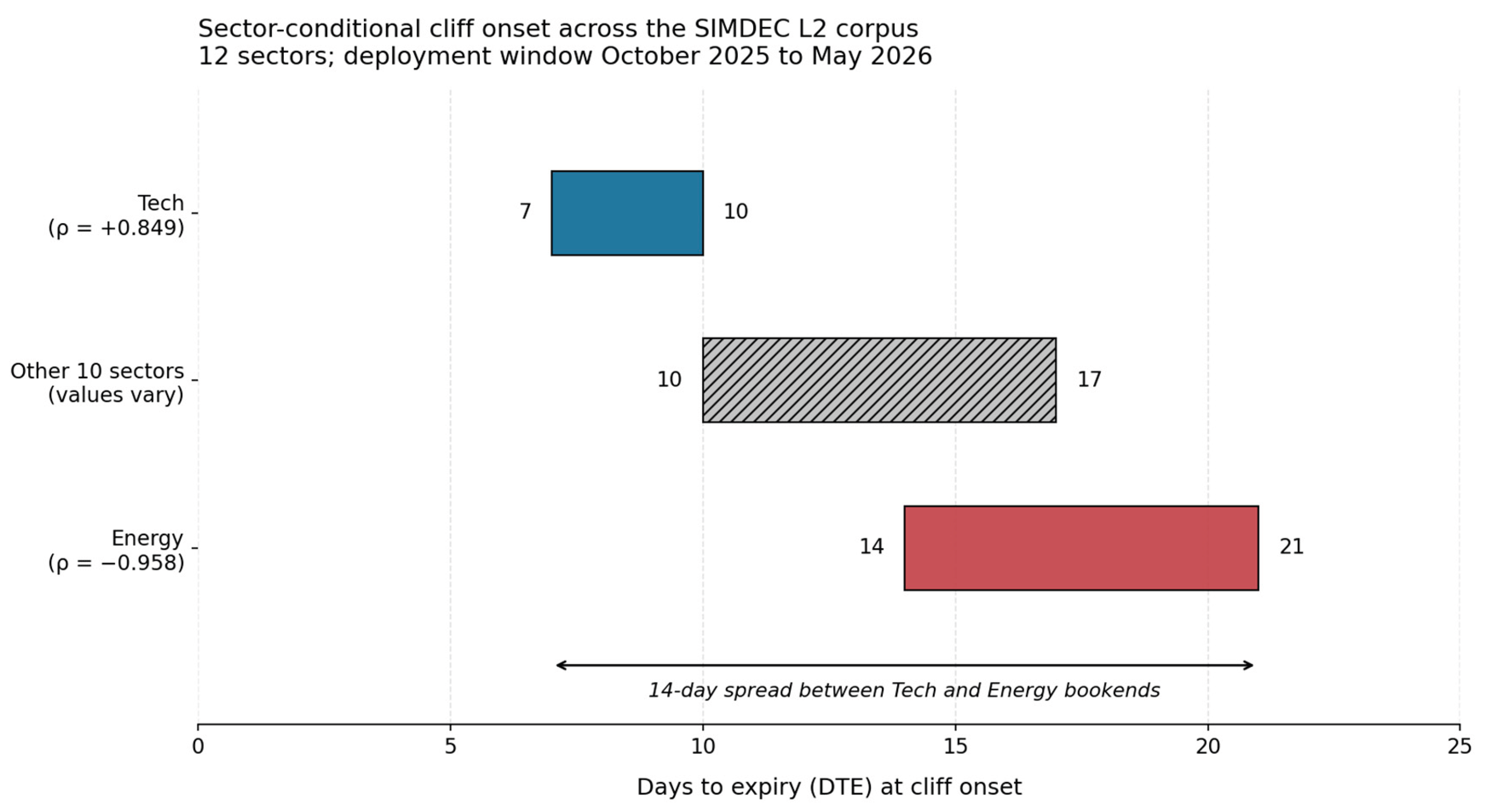
Table 1.
Eleven-snapshot intraday trajectory of the three-position cohort, 1 May 2026.
| Snapshot | XOM 160C (USD) | CVX 175C (USD) | LNG 250C (USD) | Notes |
| T1 (~09:35 EDT, open) | 0.45 | 0.85 | 0.70 | Session open marks |
| T2 (~10:55 EDT) | 0.07 | 0.14 | 0.11 | First cliff acceleration interval |
| T3 | 0.06 | 0.12 | 0.10 | |
| T4 | 0.05 | 0.10 | 0.08 | |
| T5 | 0.04 | 0.08 | 0.06 | |
| T6 | 0.03 | 0.06 | 0.04 | |
| T7 | 0.03 | 0.05 | 0.03 | |
| T8 | 0.02 | 0.04 | 0.03 | |
| T9 | 0.02 | 0.03 | 0.02 | |
| T10 | 0.01 | 0.02 | 0.01 | |
| T11 (~15:55 EDT, close) | 0.01 | 0.01 | 0.01 | Session close marks |
Table 2.
Variance contributions in the 4-input Sobol decomposition with regime as an explicit input. All values as percentages of total corpus variance.
Table 2.
Variance contributions in the 4-input Sobol decomposition with regime as an explicit input. All values as percentages of total corpus variance.
| Component | Variance (%) | Interpretation |
| Quality (unconditional main effect) | 30.43 | Quality alone in the 4-input setup |
| Regime (main effect) | 21.85 | Regime alone |
| Quality × Regime joint contribution | 31.64 | Joint with interaction |
| Quality conditional on regime (mean across regimes) | 16.80 | Within-regime variance, averaged |
| Conditional drop | 13.63 pp | 45% reduction |
Disclaimer/Publisher’s Note: The statements, opinions and data contained in all publications are solely those of the individual author(s) and contributor(s) and not of MDPI and/or the editor(s). MDPI and/or the editor(s) disclaim responsibility for any injury to people or property resulting from any ideas, methods, instructions or products referred to in the content. |
© 2026 by the authors. Licensee MDPI, Basel, Switzerland. This article is an open access article distributed under the terms and conditions of the Creative Commons Attribution (CC BY) license.
Copyright: This open access article is published under a Creative Commons CC BY 4.0 license, which permit the free download, distribution, and reuse, provided that the author and preprint are cited in any reuse.


