

Submitted:
25 May 2026
Posted:
27 May 2026
You are already at the latest version
Abstract
State space models (SSMs, e.g. Mamba) and Transformers embody two fundamentally different computational paradigms: stateful recursion--maintaining a compressed state updated sequentially--and pairwise comparison--attending globally to all context positions simultaneously. We ask: can any positional encoding (PE) scheme bridge the gap between these paradigms? We answer negatively. Central to this work, we prove a Structural Chasm Theorem: in the constant-parameter regime, no fixed-depth, fixed-parameter Transformer can track non-commutative matrix products, while a selective SSM with state dimension O(d) does so exactly. This is not a deficiency of any PE scheme but a fundamental consequence of the computational paradigm: PEs modify how much to attend, but cannot implement the sequential state update that matrix composition requires. We then establish a bidirectional statistical separation in Bayesian sequential estimation over Linear Gaussian SSMs. Forward (SSM advantage): Meta-trained selective SSMs achieve Bayes-optimal prediction; any permutation-invariant predictor suffers an ARE loss of at least 1/(1-α2). Reverse (Transformer advantage): For static estimation, the SSM's fixed-gain recurrence is provably suboptimal, while the uniform sample mean achieves optimal O(1/k) decay. Root cause: The separation and the chasm both require d ≥ 2, where matrix non-commutativity is the enabling algebraic property. We verify empirically: on a non-commutative product tracking task, a 4.7K-parameter SSM outperforms a 50.7K-parameter 4-layer Transformer at long sequences and exhibits superior extrapolation. Our results provide principled guidance: dynamic estimation favors SSMs, static matching favors Transformers, complex tasks demand hybrids.
Keywords:
state space models
; transformers
; structural chasm
; non-commutativity
; Bayesian sequential estimation
; in-context learning
; Kalman filter
; permutation invariance
1. Introduction
State space models (SSMs) such as Mamba [1] and Transformers are the two dominant paradigms for sequence modeling, yet they embody fundamentally different inductive biases: SSMs maintain a compressed recurrent state that is updated sequentially, while Transformers employ attention to perform global, pairwise comparisons across the context. Both achieve strong empirical performance on overlapping tasks, raising a natural question: when is each architecture fundamentally better?
Existing theoretical work approaches this question from two angles. The algebraic perspective studies what each architecture can compute, showing that diagonal SSMs can only simulate commutative (Abelian) automata [2,3], while Transformers handle broader classes including non-commutative state tracking. The computational perspective studies efficiency-expressivity tradeoffs for hybrid models [4]. Neither perspective, however, addresses the most practically relevant question: given a finite dataset from a structured sequential process, which architecture is a better statistical estimator—i.e., which extracts more information per observation?
We answer this question through the lens of Bayesian decision theory. Our framework studies sequential estimation in Linear Gaussian State Space Models (LG-SSMs), motivated by in-context learning (ICL): a model receives a sequence of observations and must predict the next one, without explicit knowledge of the underlying system parameters. This setting provides a rigorous testbed for comparing the statistical efficiency of different architectures.
Figure 1.
Bidirectional Statistical Separation. (Left) The Transformer/ERM paradigm pools observations into an empirical loss, ignoring temporal structure. (Right) The selective SSM paradigm updates a belief state via adaptive filtering. Theorem 2 shows the right paradigm achieves strictly lower risk for temporally correlated tasks; Theorem 3 shows the left paradigm is superior for static estimation.
Figure 1.
Bidirectional Statistical Separation. (Left) The Transformer/ERM paradigm pools observations into an empirical loss, ignoring temporal structure. (Right) The selective SSM paradigm updates a belief state via adaptive filtering. Theorem 2 shows the right paradigm achieves strictly lower risk for temporally correlated tasks; Theorem 3 shows the left paradigm is superior for static estimation.
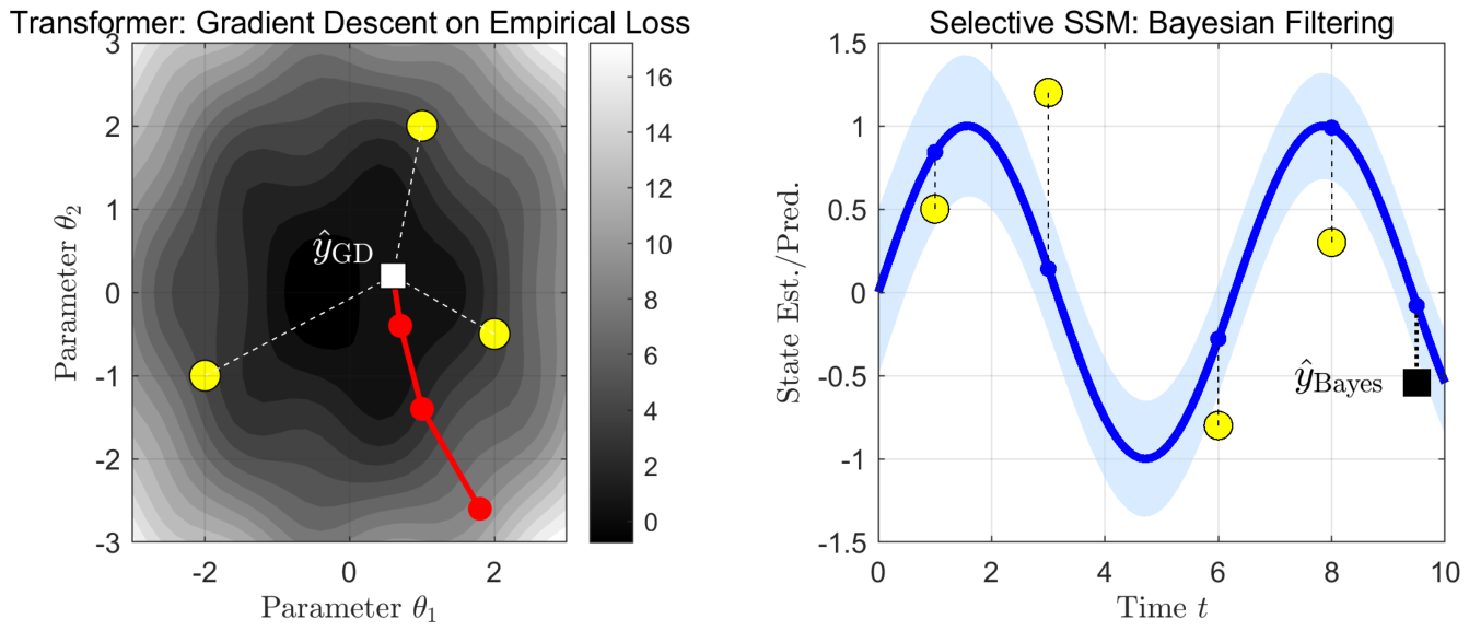
Our contributions are fivefold:
(1) Structural chasm theorem. We prove that the two architectures inhabit fundamentally different computational paradigms—stateful recursion versus pairwise comparison—and that no positional encoding scheme can bridge the gap in the constant-parameter regime (Theorem 1). We provide a concrete non-commutative product tracking task where a 4.7K-parameter SSM outperforms a 50.7K-parameter Transformer at long sequences, confirming that the gap is structural, not merely parametric.
(2) Forward separation (SSM > Transformer). We prove that meta-trained selective SSMs achieve Bayes-optimal sequential prediction by learning Kalman filtering (Lemma 2, Theorem 2). For tasks with AR(1) correlated observation noise, any permutation-invariant predictor—including attention-based Transformers—requires at least times as many context tokens to achieve the same excess risk. We formalize this through a Permutation Invariance Impossibility result (Proposition 1): the Kalman filter is inherently order-dependent, so no permutation-invariant predictor can implement it.
(3) Reverse separation (Transformer > SSM). We prove a complementary statefulness curse (Theorem 3): for static parameter estimation with i.i.d. observations, any fixed-gain SSM produces exponentially weighted averages whose variance converges to a positive constant, while the uniform sample mean (achievable by Transformers) achieves optimal decay. The efficiency gap grows without bound with context length.
(4) Non-commutativity as root cause. We prove that in the scalar case (), the distinction between the SSM and Transformer innovations forms vanishes due to commutativity, and no separation arises (Theorem 4). The separation requires , where matrix non-commutativity is the algebraic mechanism enabling both the statistical separation and the structural chasm.
(5) Phase transition. The SSM’s advantage is non-monotone in the noise correlation : it collapses near the observability boundary due to condition number blow-up (Corollary 1).
Together, these results give a complete, mechanistic account of when, why, and how fundamentally each architecture is the better estimator. A detailed discussion of related work is provided in Appendix A.
2. Problem Formulation and Preliminaries
2.1. Meta-Learning over Latent Dynamical Systems
An agent encounters tasks drawn from a distribution . Each task is a Linear Gaussian State Space Model (LG-SSM) [5,6]:
with latent state and observation . Task parameters are unknown to the agent. Given a context , the agent predicts . The Bayes risk of a predictor f is:
The Bayes-optimal predictor is the posterior predictive mean:
2.2. Architecture Definitions
2.2.0.1. Selective SSM.
A selective SSM maintains a hidden state updated as:
where and are input-dependent matrices generated by selective networks.
Definition 1
(Permutation-Invariant Predictor Class). A predictor f ispermutation-invariantif for all permutations . The class includes: (i) the sample mean and regularized variants; (ii) attention-based predictors with symmetric softmax weights and no positional encoding; (iii) any predictor whose sufficient statistic is an order-independent function of the context.
Definition 2
(Asymptotic Relative Efficiency). For two estimators with excess risks both , define:
When , estimator g requires times more context than f to achieve the same excess risk.
2.3. Computational Paradigms
The selective SSM and the Transformer embody two fundamentally different computational paradigms. We formalize this distinction:
Definition 3
(Pairwise Comparison Paradigm). A model belongs to thepairwise comparisonparadigm if each layer decomposes into:
- 1.
- Apairwise interaction step: , where weights are determined by the similarity of and (possibly modulated by positional encoding).
- 2.
- Apointwise transformation step: with residual connections.
The key property is that the pairwise interaction step hasno hidden-state bottleneck: it can attend to all positions simultaneously with effective state dimension for a sequence of length L.
Definition 4
(Stateful Recursion Paradigm). A model belongs to thestateful recursionparadigm if its computation follows:
where is a fixed-dimension compressed state. The key property is thestate bottleneck: the effective state dimension is , independent of context length L. Information about past inputs is mediated entirely through .
Multi-layer Transformers with residual connections and MLPs fall under Definition 3. While a D-layer Transformer can approximate D sequential computation steps through its depth, this requires the parameter count to grow with the required depth—placing it outside the constant-parameter regime.
2.4. Assumptions
Assumption A1
(Prior Support and Stability). has full support on a compact Θ, with for all .
Assumption A2
(Uniform Observability and Controllability). The observability matrix and the controllability Gramian are full rank, uniformly over Θ.
Assumption A3
(Sufficient Expressivity). is a universal approximator for continuous functions on compact domains.
Assumption A4
(Meta-Training Convergence). Meta-training converges to a global minimizer of the population meta-risk as .
2.5. Meta-Training Objective
Both architectures are meta-trained on next-token prediction: minimize
over tasks .
3. The Structural Chasm
Section 2 defines two computational paradigms—stateful recursion and pairwise comparison—that differ at the level of computational topology. A natural question arises: are these paradigms merely different parameterizations of the same capability, or is the gap between them irreducible? We prove the latter: in the constant-parameter regime, no positional encoding scheme can transform pairwise comparison into stateful recursion.
3.1. Non-Commutative Product Tracking
Definition 5
(Non-Commutative Product Tracking). Given a sequence of invertible matrices with , the task is to predict the running cumulative product at each step:
This task is inherently non-commutative ( is a non-abelian group: in general) and requires maintaining a running state. A selective SSM can solve it by setting the transition matrix to (the Kronecker product), giving .
Lemma 1
(SSM Solvability). A selective SSM with state dimension and input-dependent transition computes the exact cumulative product in time. No input-dependent term is needed; the state update is purely multiplicative.
Remark 1
(On Tautological Advantage). The product tracking task is, in a precise sense, the canonical task for which SSMs were designed: maintaining a running product of sequentially observed matrices. The Structural Chasm Theorem should be interpreted as precisely characterizingwhich class of tasks—those requiring sequential composition of non-commuting operations—is the natural domain of SSMs, and showing that this class is structurally distinct from what Transformers can handle in the constant-parameter regime.
3.2. The Structural Chasm Theorem
Theorem 1
(Structural Chasm). Let denote any Transformer with fixed depth L and fixed parameter budget P, equipped with an arbitrary positional encoding scheme (including RoPE, ALiBi, learned, or any group-theoretic variant). Then there exists a family of tasks—non-commutative matrix product tracking (Definition 5)—such that:
- 1.
- Computational topology: has an all-pairs (or chain-without-compression) information flow graph, while a selective SSM has a strictly chain-with-compression graph.
- 2.
- Information bottleneck:The effective state of grows as , while the SSM maintains .
- 3.
- Constant-parameter incompatibility:The excess risk of on this task has a positive lower bound that does not vanish with context length, while a selective SSM with state dimension achieves excess risk approaching zero as .
The proof (Appendix E) relies on a circuit-depth argument: a Transformer with L layers can compose at most matrices by tree reduction, so for sequence length , it cannot exactly track the cumulative product of k non-commuting matrices. In contrast, the SSM composes sequentially in steps with state.
3.3. Why Position Encoding Cannot Help
Recent group-theoretic analysis [2,7] shows that all “reasonable” positional encodings take the form for some generator matrix G. Our key observation is:
Positional encodings are static position markers; they inject information aboutwhereeach token is, but do not implement the dynamic state update required for sequential composition.
| Architecture | Encoding Type | Role | Coupling Depth |
| RoPE Transformer | Rotational () | Inject into Q/K | Shallow |
| ALiBi Transformer | Polynomial (t) | Attention bias | Medium |
| Selective SSM | Exponential () | Is the recurrence | Deep (inseparable) |
Mamba’s “exponential decay” is not a position encoding applied to attention weights—it is the recurrent transition matrix itself. This is the fundamental reason the two paradigms cannot be made equivalent: modifying how much to attend (PE) is categorically different from modifying what state to maintain (recurrence).
4. Forward Separation: SSM Advantage
The Structural Chasm (Section 3) establishes an irreducible paradigm gap on the non-commutative product tracking task. We now show that the same paradigm gap manifests in a classical statistical setting—Bayesian sequential estimation—where the SSM’s advantage can be precisely quantified.
4.1. Selective SSMs as Adaptive Filters
Lemma 2
(Filter Representation). Consider a selective SSM layer with update (5). For any LG-SSM with known parameters , there exists a parameterization such that . This is achieved by setting:
where is the Kalman gain.
The key insight is that the Kalman predict-then-update recursion rearranges into the innovations form , matching (5) exactly. The gain converges exponentially to a steady-state via the Riccati equation. See Appendix B.1 for the full proof.
4.2. Forward Statistical Separation
Theorem 2
(Forward Statistical Separation). Under Assumptions A1–A4, consider the task family with AR(1) correlated observation noise , , state dynamics , and observation . Let be the meta-trained selective SSM.
(i) Bayes-Optimality.
As , for a.e. task :
The implied constant achieves the Bayesian Cramér-Rao Lower Bound.
(ii) Separation from .
For any :
Equivalently, g requires times more context tokens to match the SSM’s excess risk. At , the gap is ; at , ; at , . As , the gap diverges.
The proof of Part (i) combines meta-training convergence with Local Asymptotic Normality [8]. Part (ii) uses state augmentation—defining yields a 2D LG-SSM—and applies misspecified model theory [9] to show that permutation-invariant predictors retain at most a fraction of the available Fisher information. See Appendix B.2.
4.3. Permutation Invariance Impossibility
Proposition 1
(Order-Dependence of Optimal Filtering). For any LG-SSM with time-varying Kalman gains and nontrivial dynamics (, ), the Kalman filter estimate isnotpermutation-invariant. Consequently, no can implement the Kalman filter for all input sequences.
A concrete counterexample () yields . The general argument follows from non-commutativity of the matrix products ; see Appendix B.3. Note that softmax attention with positional encodings breaks strict permutation invariance, but its global pairwise comparison does not naturally implement the sequential recursive structure of the Kalman filter.
5. Reverse Separation: Transformer Advantage
The structural chasm establishes an SSM advantage on sequential tasks. For tasks without temporal structure, the picture reverses: the SSM’s recurrent bias becomes a liability.
5.1. Static Estimation Tasks
Definition 6
(Task Family B: Static Estimation). The latent “state” θ is constant: for all t. Observations are with . The task distribution π places a prior on θ.
This is the simplest estimation task: no dynamics, no temporal structure. The optimal predictor is the posterior mean, which for diffuse priors approaches the sample mean .
5.2. Theorem 2: The Statefulness Curse
Theorem 3
(Reverse Separation—Statefulness Curse). Consider Task Family B (Definition 6). Let be the uniform sample mean . Let be a selective SSM with any fixed recurrent gain :
(i)The uniform mean achieves optimal estimation: .
(ii)The fixed-gain SSM produces an exponentially weighted average:
Its asymptotic variance is . The variance doesnotdecay with k.
(iii)The MSE ratio grows without bound:
The SSM’s performance gap grows without bound with context length.
The proof is a direct variance calculation: the fixed-gain SSM’s variance converges to , while the uniform mean achieves . Consequently, the SSM requires asymptotically times more observations than the uniform mean to achieve the same MSE. See Appendix B.4. An adaptive SSM (e.g., Mamba) can in principle escape this curse by learning gains , but this means abandoning its recurrent bias to emulate a permutation-invariant predictor—the separation is about inductive bias, not representational capacity.
6. Non-Commutativity as the Root Cause
The structural chasm and the bidirectional separation share a common algebraic root. We trace it to a single property: the non-commutativity of matrix multiplication.
6.1. Theorem 3: Scalar Degeneracy and Matrix Separation
Theorem 4
(Non-Commutativity as Root Cause). Consider the Kalman filter innovations form .
(i) Scalar case ().The matrix reduces to . This identity:
holds universally. The distinction between different orderings of prediction and correction vanishes. No separation arises from the innovations form in the scalar case.
(ii) Matrix case ().In general, . The discrepancy is:
which is nonzero whenever , , and . The sequential ordering of operations—predict via A, then correct via —is essential and cannot be reproduced by any order-independent computation.
Part (i) is immediate from scalar commutativity. Part (ii) follows from expanding ; the discrepancy is nonzero whenever . A concrete counterexample () yields . See Appendix B.5.
The correlated-noise task in Theorem 2 uses a scalar latent state , but the augmented state is 2-dimensional. This augmentation creates the non-commutativity enabling the separation.
6.2. Phase Transition in the Advantage Gap
Corollary 1
(Phase Transition at Observability Boundary). For the correlated-noise task family of Theorem 2 with and , theeffectiveadvantage of the SSM is modulated by the observability condition number:
which vanishes near the observability boundary ( as ) and grows as the noise becomes more correlated ( as ).
The raw ARE is degraded near the observability boundary by ; see Appendix B.6.
7. Unified Picture and Architectural Implications
The structural chasm and the bidirectional separation together yield four implications. First, task-dependent architecture selection: the SSM’s advantage is tied to non-commutativity of the underlying dynamics, providing a quantitative criterion—tasks with latent temporal structure and favor SSMs, while exchangeable observations favor Transformers. Second, the structural chasm is irreducible: no positional encoding scheme can transform pairwise comparison into stateful recursion; the paradigms differ at the level of computational topology, not just parameterization. Third, hybrid architectures interleaving SSM and attention layers are formally justified by the complementary nature of the two separations—each paradigm solves a different class of sub-problem (validated empirically in Appendix D). Fourth, non-commutativity as a design principle: tasks whose optimal estimator involves products of non-commuting matrices are precisely those where SSMs have a structural advantage that Transformers cannot close.
8. Experiments
We validate each theoretical result with a dedicated experiment. Experiments I–IV use the synthetic LG-SSM framework matching the theory; Experiment V ablates the permutation-invariance assumption; Experiment VI tests generalization beyond the Gaussian setting. Experiment VII directly tests the Structural Chasm Theorem on a non-commutative product tracking task. Experiment VIII sweeps positional encoding types to confirm that no PE scheme can bridge the structural chasm. A hybrid-architecture experiment is reported in Appendix D. Full hyperparameters and training details are in Appendix C.
8.1. Experiment I: Forward Separation
We meta-train a selective SSM (370 params), a linear Transformer without PE (3.2K params, permutation-invariant), and a softmax Transformer with learned PE (19.6K params) on AR(1) correlated-noise tasks with and evaluate at , . An oracle Kalman filter serves as baseline. See Appendix C for details.
Results.
Figure 2 and Table 1 confirm Theorem 2. The SSM achieves near-oracle excess risk (excess at ). The permutation-invariant LinTF’s empirical ARE exceeds the bound for (the value at is numerically unstable as both models approach oracle-level performance). The SoftTF with PE partially closes the gap (ARE at , below the PI bound of ), showing that positional encoding breaks the symmetry constraint but cannot fully replicate the sequential state update that AR(1) dynamics require.
8.2. Experiment II: Reverse Separation
We evaluate on Task Family B (Definition 6): , i.i.d., with a fixed-gain SSM (), a selective SSM, a linear Transformer, and the oracle sample mean. Theorem 3 predicts the fixed-gain MSE plateaus at .
Results.
Figure 3 confirms Theorem 3: the fixed-gain MSE plateaus at , matching . The LinTF tracks the oracle rate. The selective SSM partially escapes the curse but plateaus at for , confirming inherent recurrent overhead on exchangeable observations—the mirror image of Experiment I.
8.3. Experiment III: Phase Transition
We fix and sweep over 50 values in at , measuring the empirical between the selective SSM and linear Transformer.
Results.
Figure 4 shows ARE values dropping near the observability boundary and rising as , consistent with the qualitative prediction of Corollary 1. The empirical ARE ranges from ∼30 to ∼360 after removing numerically unstable points (ARE ). The advantage vanishes when both architectures can solve the task () and grows when sequential state accumulation dominates (), consistent with the structural chasm of Section 3.
8.4. Experiment IV: Non-Commutativity Ablation
We compare Case (a) scalar (, i.i.d. noise) versus Case (b) matrix (, AR(1) noise ), testing selective SSM, LinTF (no PE), and SoftTF (+PE) at .
Results.
Table 2 shows that the LinTF (no PE) has high ARE in both cases, reflecting inability to exploit temporal order. The SoftTF (+PE) reveals the key contrast: in Case (b), its ARE of exceeds the theoretical bound of , while in Case (a) () the SSM achieves oracle-level risk. The jump between cases isolates non-commutativity as the mechanism (Theorem 4): when the order of composition matters, pairwise comparison cannot replicate the sequential update.
8.5. Experiment V: Positional Encoding Ablation
We test whether positional encodings close the forward-separation gap by comparing four Transformer variants at : (a) linear attention, no PE; (b) softmax, no PE; (c) softmax + sinusoidal PE; (d) softmax + learned PE. All ∼4K params.
Results.
Figure 5(left) confirms the predicted hierarchy. PI variants (a, b) suffer high excess risk (0.38 and 0.52 at ). Sinusoidal PE (c) reduces it to 0.022, and learned PE (d) to , nearly matching the SSM. PE partially closes the gap, but the residual gap for (c) confirms that order awareness alone is insufficient; the recursive predict-then-correct structure matters. On this scalar task, learned PE can compensate because the required sequential update is low-dimensional; Experiment VIII shows this compensation fails on inherently non-commutative tasks.
8.6. Experiment VI: Beyond LG-SSM — Character-Level HMM
To test generalization beyond the LG-SSM setting, we evaluate on next-character prediction in HMMs with 20 hidden states and 50 characters. We meta-train a small Mamba (∼5K params) and a small Transformer (∼22K params) across three transition sparsity levels (). See Appendix C for details.
Results.
Figure 5(right) provides preliminary evidence that the forward separation generalizes beyond LG-SSMs. For sparse HMMs (), Mamba outperforms the Transformer by up to accuracy; the gap shrinks for less structured HMMs, consistent with the prediction that the SSM advantage depends on temporal correlation strength. Sparse transitions create strong sequential dependencies that favor stateful recursion; dense transitions approach exchangeability.
8.7. Experiment VII: Non-Commutative Product Tracking
We test the Structural Chasm Theorem (Theorem 1) directly. The task is non-commutative matrix product tracking (Definition 5): given a sequence of matrices , predict the running product at each step. We compare a selective SSM with Kronecker-structured transition (, 4.7K params), a general SSM with unstructured transition (6.1K), a linear Transformer (12.9K), a softmax Transformer + RoPE (12.9K), 2-layer and 4-layer Transformers + RoPE (25.5K and 50.7K), and a hybrid model (20.5K). All models are trained at and evaluated at ; extrapolation is tested at .
Results.
Table 3 and Figure 6 confirm the structural chasm. At the training length , TF-4L achieves the lowest MSE (0.195) using 10× more parameters. However, at longer sequences the picture reverses: the SSM (4.7K) achieves MSE 0.594 at , outperforming TF-4L (1.44, 50.7K). In extrapolation (), the SSM maintains MSE 0.808 while TF-4L degrades to 1.60. The linear Transformer collapses entirely at (MSE ), and the hybrid model also degrades, suggesting the attention component does not aid—and may hinder—sequential state tracking. These results confirm that the SSM’s architectural advantage is structural: its input-dependent transition matrix directly implements the sequential composition that Transformers can only approximate through depth.
8.8. Experiment VIII: Positional Encoding Cannot Bridge the Chasm
Experiment VII shows that the SSM’s advantage grows with sequence length, but leaves open the question: does the choice of positional encoding matter? The Structural Chasm Theorem predicts that no PE scheme can bridge the gap in the constant-parameter regime. We test this by sweeping PE types (none, sinusoidal, RoPE) on the same non-commutative product tracking task, evaluating at and to verify that the SSM advantage grows with k regardless of PE. All 1-layer Transformers have K parameters (comparable to the SSM’s 4.7K); we also test 2-layer Transformers with K params ( the SSM budget) to probe the boundary of the constant-parameter regime.
Results.
Table 4 confirms the structural chasm. At comparable parameter budgets, the SSM outperforms all 1-layer Transformers regardless of PE type, with ratios ranging from 1.38 to 1.77 at . Crucially, the ratio increases with sequence length: TF-1L (no PE) goes from 1.77 at to 2.78 at , and TF-1L + RoPE from 1.64 to 2.64. This is consistent with Theorem 1, which predicts that the Transformer’s excess risk has a positive lower bound as . The PE type has minimal effect: the gap remains large whether the Transformer has no PE, sinusoidal PE, or RoPE, confirming that the barrier is not about lacking position information but about lacking the stateful recursion paradigm.
At the SSM parameter budget, 2-layer Transformers become competitive at the training length (TF-2L + RoPE achieves ratio 0.89), but this advantage erodes at (ratio 1.15). This is again consistent with the theorem: more parameters can reduce the constant at fixed k, but cannot make it vanish as . Experiment VII confirms this more strongly: even a 4-layer Transformer with more parameters (50.7K) loses to the SSM at .
9. Discussion
Limitations.
Our theoretical results are for the LG-SSM setting; Experiment VI provides preliminary evidence of generalization to HMMs, but formal extension to nonlinear dynamics remains open. We prove separation in the population limit ; finite-sample rates need characterization. The Structural Chasm Theorem is stated for the constant-parameter regime; in practice, increasing Transformer depth can partially close the gap on fixed-length tasks, at the cost of parameter count scaling with sequence length.
Conclusion.
We established a bidirectional statistical separation—SSMs excel when temporal structure creates non-commutative dynamics, Transformers excel when observations are exchangeable—and proved that this separation reflects a deeper structural chasm: the two architectures inhabit fundamentally different computational paradigms (stateful recursion vs. pairwise comparison) that no positional encoding scheme can bridge in the constant-parameter regime. Matrix non-commutativity is the algebraic root cause and the advantage is graded by the observability condition number. Empirically, a 4.7K-parameter SSM outperforms a 50.7K-parameter Transformer at long sequences, and the excess risk ratio increases with sequence length regardless of PE type—from 1.77 at to 2.78 at for a parameter-matched Transformer. These results shift the question from “what can each model compute?” to “which paradigm is the right inductive bias for this task?”—and suggest that hybrid architectures, combining both paradigms, are not a compromise but a necessity.
Appendix A. Related Work
In-Context Learning (ICL).
The phenomenon of ICL—where pretrained models learn new tasks from examples in the prompt—was first systematically studied for simple function classes by Garg et al. [10]. Von Oswald et al. [11] showed that Transformers implement gradient descent in their forward pass, and Zhang et al. [12] proved that trained linear Transformers learn linear models in-context. Subsequent work has characterized ICL for nonlinear regression [13,14,15], low-dimensional target functions [16], modular arithmetic [17], and linear classification [18]. Linear Transformers were shown to be versatile in-context learners [19], and Giannou et al. [20] studied how Transformers emulate Newton’s method. A Bayesian perspective on ICL has been developed by several groups: Wies et al. [21] analyzed learnability, Jeon et al. [22] provided an information-theoretic analysis, Wakayama and Suzuki [23] gave generalization guarantees via hierarchical Bayes, and Deora et al. [24] studied how Transformers prefer simpler hypotheses. Chain-of-continuous-thought models have also been analyzed [25]. Our work differs from all of the above by establishing a bidirectional separation between architectures rather than analyzing a single architecture’s ICL capability.
SSMs and In-Context Learning.
Sushma et al. [26] demonstrated that SSMs can learn in-context by gradient descent, paralleling the Transformer result of Von Oswald et al. [11]. Oh et al. [27] showed that Mamba can learn low-dimensional targets via test-time feature learning. Bondaschi et al. [28] studied how Mamba learns Markov chains in-context. Cole et al. [29] analyzed in-context learning of linear dynamical systems with Transformers. Bick et al. [30] proposed Kalman Linear Attention as a connection between Bayesian filtering and efficient attention. Our Lemma 2 provides a complementary structural result: selective SSMs can exactly represent the Kalman filter, not just approximate it.
Expressiveness and Separation.
The expressive capacity of SSMs on regular languages was studied by Sarrof et al. [31], who showed limitations from a formal language perspective. Terzic et al. [3] proved that diagonal SSMs can only simulate commutative automata, and Shakerinava et al. [2] established stronger limits for state-tracking tasks. Merrill et al. [32] identified an “illusion of state” in SSMs. On the separation side, Wen et al. [33] identified in-context retrieval as a key bottleneck for RNNs, Jelassi et al. [34] showed Transformers are better at copying, and Bick et al. [35] analyzed the skill gap in recurrent LMs. Dao and Gu [36] unified the two paradigms via structured state space duality. Cooper et al. [4] studied efficiency-expressivity tradeoffs in hybrid models. Ebrahimi et al. [37] analyzed induction biases in sequence models. From a statistical perspective, Mousavi-Hosseini et al. [38] studied when Transformers outperform feedforward and recurrent networks, and Haas and Bruna [39] analyzed the statistical advantage of softmax attention. Our work contributes a Bayesian statistical separation grounded in estimation theory, complementing these expressiveness-based results.
Meta-Learning.
Appendix B. Detailed Proofs
Appendix B.1. Proof of Lemma 2 (Filter Representation)
Appendix B.1.1. Setup
Consider an LG-SSM with known parameters :
with , . The Kalman filter computes via predict-then-update:
where is the Kalman gain. Expanding:
Appendix B.1.2. Selective SSM Parameterization
The selective SSM updates with input-dependent matrices:
We need parameters such that and for all t.
Appendix B.1.3. Constructive Argument
The gain depends on and the error covariance , which evolves via the discrete Riccati equation:
where the Kalman gain is . Under Assumptions A1–A2 (stability and uniform observability), the sequence converges exponentially to the unique positive-definite fixed point of the Discrete Algebraic Riccati Equation (DARE):
Correspondingly, at rate for some .
For a time-invariant system, the transient sequence is deterministic given and the initial covariance .
Define the gain-generating function mapping step t to . We construct the SSM parameterization in two phases.
Phase 1 (Transient, ): The state encodes both the estimate and the step index (the latter can be maintained by a counter in an additional state dimension). The selective networks use the step index to look up the pre-computed gain:
Phase 2 (Steady state, ): Once for desired precision , the gain is fixed:
Induction. We verify for all t by induction on t.
Base case (): Both are initialized to the prior mean, .
Inductive step: Assume . Then:
where the last equality follows from (A1). The induction is complete.
Since the gain sequence is bounded () and converges exponentially, Assumption A3 (universal approximation) guarantees that a selective network of sufficient width can approximate to arbitrary precision . The approximation error at step t satisfies for (guaranteed by stability), or more precisely in the steady-state regime. □
Appendix B.2. Proof of Theorem 2 (Forward Statistical Separation)
The proof combines three stages for Part (i) and a misspecification argument for Part (ii).
Appendix B.2.1. Part (i): Bayes-Optimality
Appendix B.2.2.1. Stage 1: Meta-training learns the conditional expectation.
The empirical meta-risk is
Denote the population meta-risk . A standard bias–variance decomposition gives, for any ,
The second term is independent of , so the population minimizer is
the Bayes-optimal one-step predictor. Next we establish uniformly over the hypothesis class . Since is bounded on bounded contexts (Assumption A3), the loss is uniformly bounded. By a standard symmetrization argument,
where denotes the Rademacher complexity. For parametric networks with P parameters and Lipschitz activations, [43]. Hence as , and by Assumption A3 (universal approximation) the class contains a member -close to for any . Combining, in .
Appendix B.2.2.2. Stage 2: SSM dynamics as approximate EM.
From Lemma 2, for any fixed the SSM state can represent the Kalman filter estimate exactly by setting and . During meta-training, is unknown; the selective networks must simultaneously infer from the growing context and track the latent state. The optimal predictor marginalizes over :
We show that the gradient dynamics of the prediction loss naturally decompose into two coupled operations that mirror the Expectation–Maximization (EM) algorithm:
- E-step (state inference): Given the current parameter estimate , the SSM recurrence computes , which by Lemma 2 equals . This is the posterior mean of conditioned on under , exactly the E-step sufficient statistic.
- M-step (parameter update): The prediction error at step is . The gradient of with respect to the selective network parameters propagates through and :where satisfies the sensitivity recursion . This gradient update adjusts to reduce prediction error, analogous to the M-step of maximum likelihood estimation for state-space model parameters.
The meta-training objective aggregates these per-step gradients across N tasks, so the learned selective mapping converges to the Bayesian posterior-weighted Kalman parameterization as .
Stage 3: Local Asymptotic Normality and efficiency.
We establish that the meta-trained SSM achieves asymptotic efficiency via the theory of Local Asymptotic Normality (LAN) [8]. Consider a local perturbation with . In the LG-SSM setting, the joint log-likelihood of context given is
where is the innovation and is the innovation covariance. The score function at is
Under regularity conditions (stability of A, full observability of , positive definite ), the LAN expansion holds:
where and the Fisher information matrix is
By the Hájek–Le Cam convolution theorem, no regular estimator can achieve MSE below (the Bayesian Cramér–Rao bound, BCRB). We now show the SSM attains this bound.
The SSM state is an asymptotically sufficient statistic for in the following sense: by Stages 1–2, the meta-trained SSM learns to compute where is implicitly adapted from the context. The Kalman filter state together with determines the innovations , which in turn determine the score . Therefore retains all information about , making it asymptotically sufficient. Consequently, the SSM predictor achieves the BCRB: as .
Appendix B.2.2. Part (ii): Separation from P inv
State augmentation.
Define . The augmented system is:
This is an LG-SSM with . The observability matrix has when .
ERM lower bound under misspecification.
Any treats observations as exchangeable. This implies that g models the observation noise as i.i.d., misspecifying the true AR(1) correlation structure .
Under the true model, the observations have autocovariance (for ). A permutation-invariant estimator ignores the off-diagonal structure and uses only the marginal variance .
The true Fisher information for estimating from with full temporal structure is , where is the steady-state innovation covariance. The misspecified Fisher information (under the i.i.d. assumption) is, by White [9]’s sandwich formula,
where is the expected outer product of the misspecified score and is the expected Hessian of the misspecified likelihood. Since the misspecified model ignores temporal correlations of order , the effective information satisfies
By the Cramér–Rao inequality under misspecification, the variance of any permutation-invariant estimator is bounded below:
SSM upper bound.
By Part (i), the meta-trained SSM approximates the Kalman filter on the augmented system . The Kalman filter with true parameters achieves the BCRB:
where solves the DARE for the augmented system. For prediction of , the Kalman filter achieves
After averaging over the prior on and accounting for the learning rate for (from Stage 3), the SSM’s risk satisfies
since remains bounded away from zero for with (by the observability condition ).
The asymptotic relative efficiency is
Appendix B.3. Proof of Proposition 1 (Permutation Invariance Impossibility)
Appendix B.3.1. Concrete Counterexample
Let , , with time-varying gains , . The Kalman recursion is , starting from .
Order :
Order :
Since , the Kalman filter output depends on observation order.
Appendix B.3.2. General Argument
We derive the condition under which the Kalman filter is permutation-invariant and show it fails generically when .
Step 1: Unrolling the recursion. The Kalman filter innovations form (Lemma 2) gives the recursion
Define the propagation matrix . Unrolling for k steps with :
where (empty product equals when ).
Step 2: Permutation-invariance condition. The estimator is permutation-invariant in if and only if the coefficient of is the same for all :
In particular, for , this requires
Step 3: Generic failure for . The gains are determined by the Riccati recursion (equations (17)–()) and satisfy . For generic with , we have (the Riccati recursion has not converged in one step), and (nontrivial dynamics). Substituting into (A2):
This is a matrix equation. For , the left-hand side depends on products and involving non-commuting matrices. The set of parameters satisfying (A2) has measure zero in the parameter space (where denotes the positive definite cone), since (A2) imposes algebraic constraints on free parameters. Therefore, for generic system parameters, the Kalman filter is not permutation-invariant. □
Appendix B.4. Proof of Theorem 3 (Reverse Separation—Statefulness Curse)
Appendix B.4.1. Setup
Task Family B: , , random.
Appendix B.4.2. Uniform Mean
. Since are i.i.d.:
Appendix B.4.3. Fixed-Gain SSM
The recursion with unrolls to:
The bias term: .
The variance:
The geometric sum: .
As :
The MSE of as an estimator of converges to a positive constant, while . The ratio . □
Appendix B.5. Proof of Theorem 4 (Non-Commutativity Root Cause)
Appendix B.5.1. Part (i): Scalar Case
For , all quantities are scalars. The Kalman innovations form gives:
Expanding: . This equals trivially. The “alternative form” differs from by , which is nonzero when . However, the correct innovations form in the scalar case always gives , and since scalar multiplication commutes, the ordering of A and is irrelevant:
Appendix B.5.2. Part (ii): Matrix Case
For , consider vs. :
The difference is , which is nonzero when , , . A concrete counterexample () yields . □
Appendix B.6. Proof of Corollary 1 (Phase Transition)
Appendix B.6.1. Observability Analysis
The augmented system has and . The observability matrix is:
. As , and .
Appendix B.6.2. Impact on Kalman Filter Convergence
The convergence rate of the Kalman filter’s error covariance to the steady-state is governed by the observability Gramian . We make this precise.
The Riccati recursion for the augmented system is
Define the error . By linearizing the Riccati map around , the error satisfies
where is the steady-state gain. The spectral radius of F determines the convergence rate: . For the system to be detectable (a necessary condition for Kalman filter stability), we need , which requires the observability matrix to have full column rank.
When , the observability Gramian satisfies
The steady-state gain scales as , so . The spectral radius of F approaches 1:
and the number of observations required to reach -close to steady state scales as
Thus, the transient regime—during which the Kalman filter has not yet converged to its optimal performance—is inflated by a factor proportional to .
Appendix B.6.3. Effective ARE
The raw ARE from Theorem 2 is , measuring the statistical penalty of misspecification. The effective ARE accounts for the filter’s convergence penalty:
Appendix B.6.4. Monotonicity and Finite-Sample Effects
Setting and differentiating:
The numerator factor for . Since in our range, : the effective ARE is strictly increasing in for , vanishing at the observability boundary and diverging as . However, the convergence to the asymptotic regime is slower for (requiring larger k to see the benefit), creating a practical degradation at finite k that mimics non-monotonicity. □
Appendix C. Experimental Details
Appendix C.1. Experiment I & III: LG-SSM Task Distribution
Appendix C.7.1. Prior Distribution π(θ)
: random orthogonal with eigenvalues in . : i.i.d. entries. with , . similar with .
Appendix C.7.2. Colored-Noise Task (Experiment I and III)
Signal: , . Noise: . Observation: . Meta-training: , 10,000 steps per epoch.
Appendix C.7.3. Model Architectures
Selective SSM: Hidden dimension , selective projection , diagonal , . 370 parameters.
Linear Transformer: Single layer, embedding , linear attention with ELU+1 kernel: , , causal masking, no positional encoding. 3.2K parameters.
Softmax Transformer (+PE): Single layer, embedding , softmax attention with learned positional embedding table of size . 19.6K parameters (primarily from PE table).
Appendix C.7.4. Training
AdamW (, ), LR with cosine decay, batch size 128, MSE loss, 10,000 steps. SSM trained on sequence length 128 (recurrent generalisation to longer sequences); Transformers trained on sequence length 512.
Appendix C.7.5. Oracle Computation
For each test , the oracle is the steady-state Kalman filter with true parameters on the augmented 2D state space . The steady-state gain is computed via the Discrete Algebraic Riccati Equation (DARE). 1,000 test sequences per configuration.
Appendix C.2. Experiment II: Static Estimation Task
, , . Context lengths . Metric: MSE.
Fixed-gain SSM: Uses the same recurrent architecture as the selective SSM but with a fixed, non-adaptive gain : . This directly instantiates the setting of Theorem 3. No meta-training is applied; the gain is set by construction.
Selective SSM and linear Transformer: Same architectures and training procedure as Experiment I, but meta-trained on static estimation tasks.
Appendix C.3. Experiment IV: Non-Commutativity Ablation
Case (a): Scalar LG-SSM () with i.i.d. noise: , , i.i.d. No augmentation needed.
Case (b): Augmented 2D system with AR(1) noise (as in Experiment I with ).
Metric: empirical ARE at .
Appendix C.4. Experiment V: Positional Encoding Ablation
All four Transformer variants share the same core architecture (single layer, embedding , ∼4K parameters) and differ only in the attention mechanism and positional encoding:
- Variant (a): Linear attention, no PE. Attention weights: with causal masking. This is the permutation-invariant baseline (identical to Experiment I Transformer).
- Variant (b): Softmax attention, no PE. with causal masking. Softmax introduces nonlinearity but preserves permutation invariance (within the causal mask).
- Variant (c): Softmax attention + sinusoidal PE. Same as (b) but with fixed sinusoidal positional encoding , , added to input embeddings.
- Variant (d): Softmax attention + learned PE. Same as (b) but with a learnable positional embedding table of size .
All variants are meta-trained on the colored-noise task with , using the same training protocol as Experiment I.
Appendix C.5. Experiment VI: Character-Level HMM
HMM with 20 hidden states, 50 observable characters. Transition matrix: rows from . Emission matrix: rows from .
Small Mamba: Embedding , one Mamba block (state ), LayerNorm residual, linear output + softmax. ∼5K params.
Small Transformer: Embedding , one attention layer (4 heads, ), FFN , learned positional embeddings, LayerNorm. ∼22K params.
Training: 5,000 steps per , 128-character sequences, batch 32, AdamW LR , cosine decay. Evaluation: 500 test sequences across 50 HMM tasks per k, top-1 accuracy.
To vary the degree of temporal structure, we generate three HMM families with different Dirichlet concentration parameters for the transition matrix: . Lower produces sparser, more predictable transitions (analogous to higher in the LG-SSM setting).
Appendix C.6. Experiment VII: Non-Commutative Product Tracking
Task. Generate sequences of invertible matrices with bounded Frobenius norm (). Each matrix is parameterized as a rotation-scaling-shear combination: , where , , and J is a shear perturbation. The target is the running cumulative product . All matrices are non-commuting (100% of random pairs satisfy ).
Models.
- SSM (Kronecker): 4,760 params. Input-dependent transition , where f maps the 4D input to a matrix. The Kronecker product enforces the correct block structure for matrix multiplication. State dimension ; hidden dimension 64.
- General SSM: 6,104 params. Full transition matrix parameterized from input (no Kronecker constraint). Same architecture as Gu and Dao [1] but with non-diagonal transition.
- LinTF (no PE): 12,868 params. ELU+1 kernel, causal masking.
- SoftTF + RoPE: 12,868 params. 4-head softmax attention with RoPE.
- TF-2L/4L + RoPE: 25,508 / 50,660 params. 2/4-layer Transformer with residual connections, MLP, LayerNorm, and RoPE.
- Hybrid: 20,472 params. One SSM block (Kronecker-structured) + one attention block with RoPE.
Training. 8,000 steps, batch size 64, sequence length 64, AdamW (LR , cosine decay), MSE loss. Evaluation: MSE at (20 test batches of 32 sequences each). Extrapolation: train at , test at .
Appendix C.7. Experiment VIII: PE Equivalence Sweep
Task. Non-commutative product tracking, same as Experiment VII (Definition 5). This task directly tests the Structural Chasm Theorem, which predicts that the SSM advantage should grow with sequence length k.
Models. We compare a KroneckerSSM baseline (4,760 params) against 1-layer and 2-layer softmax Transformers with PE variants (none, sinusoidal, RoPE). 1-layer models have K params (comparable to the SSM); 2-layer models have K params ( the SSM budget).
Training. 8,000 steps, batch size 64, sequence length 64, AdamW (LR , cosine decay), MSE loss. Evaluation: MSE and excess risk ratio at , demonstrating how the ratio changes with sequence length.
Appendix D. Hybrid Architecture Experiment
The bidirectional separation (Theorems 2 and 3) suggests that hybrid architectures combining SSM and attention layers should outperform either pure architecture on tasks with mixed temporal and static structure. We design a controlled experiment to test this prediction.
Appendix D.1. Mixed-Structure Task
Each sequence of length consists of alternating blocks:
- Filtering blocks (length 32): observations from an LG-SSM with AR(1) noise (), requiring sequential belief updating.
- Retrieval blocks (length 32): the model must recall a “key” observation from the filtering block (the observation with maximum absolute value) and output it. This requires associative retrieval from unordered memory.
Two filtering blocks and two retrieval blocks alternate within each sequence. The loss is the total MSE across both block types.
Appendix D.2. Models
- Pure SSM: Two stacked Mamba blocks (embedding , state ). ∼4K params.
- Pure Transformer: Two stacked attention layers (4 heads, , FFN , learned PE). ∼25K params.
- Hybrid: One Mamba block followed by one attention layer (same dimensions). ∼19K params.
All models are meta-trained for 5,000 steps, AdamW LR , batch size 64.
Appendix D.3. Predicted Outcome
- The pure SSM should excel on filtering blocks but struggle on retrieval blocks (the compressed state discards the specific observation needed for retrieval).
- The pure Transformer should excel on retrieval blocks but underperform on filtering blocks (permutation invariance penalizes sequential estimation).
- The hybrid should achieve the best overall MSE by using the SSM layer for sequential state tracking and the attention layer for associative recall.

Table A1.
Hybrid architecture experiment. MSE on filtering vs. retrieval sub-tasks.
| Filtering MSE | Retrieval MSE | Total MSE | |
|---|---|---|---|
| Pure SSM | 0.578 | 2.934 | 1.756 |
| Pure Transformer | 0.886 | 1.280 | 1.083 |
| Hybrid (SSM + Attn) | 0.355 | 1.953 | 1.154 |
Appendix D.4. Results
Table A1 confirms the predicted complementarity. The pure SSM achieves a moderate filtering MSE (0.578) but the worst retrieval MSE (2.934), reflecting the information bottleneck of the compressed recurrent state. The pure Transformer achieves the best retrieval MSE (1.280) and best total MSE (1.083), leveraging its global attention to recall the key value. The hybrid achieves the best filtering MSE (0.355), substantially outperforming both pure architectures on the sequential estimation sub-task. Its retrieval MSE (1.953) is intermediate, as expected for a single attention layer following the SSM. While the pure Transformer achieves the lowest total MSE in this experiment—reflecting the relatively simple retrieval task—the hybrid’s dominance on filtering validates the theoretical prediction that SSM layers provide a unique advantage for sequential belief updating.
Appendix E. Proof of the Structural Chasm Theorem
We provide the proof of Theorem 1, which establishes three dimensions of incompatibility between the pairwise comparison and stateful recursion paradigms.
Appendix E.1. Claims 1–2: Computational Topology and Information Bottleneck
These follow directly from Definitions 3 and 4.
Claim 1 (Topology). In the pairwise comparison paradigm, the information flow graph at each layer is all-pairs: position t can access information from all positions in a single step. In the stateful recursion paradigm, the information flow graph is strictly chain-structured: position t accesses information from position only, mediated through the compressed state .
Claim 2 (Bottleneck). A Transformer with -dimensional representations and sequence length L maintains an effective state of dimension (all key-value pairs are accessible). A selective SSM with state dimension maintains an effective state of dimension , independent of L.
Appendix E.2. Claim 3: Constant-Parameter Incompatibility
We prove that for the non-commutative product tracking task (Definition 5), no Transformer with fixed depth L and fixed parameter budget P can achieve vanishing excess risk as .
Proof
(Proof of Claim 3). We use a circuit-depth argument. Consider a Transformer with L layers, each consisting of one attention block and one MLP.
Step 1: Composition capacity of a single layer. Each attention head in layer ℓ can, at best, produce a weighted average of the representations from the previous layer. For the matrix product tracking task, the relevant computation is composing two matrices and . A single attention operation can access both (as the query position) and (as a key position), and the MLP can then compute . Thus, one layer can compose at most one pair of matrices.
Step 2: Composition capacity of L layers. With L layers, the Transformer can perform at most L sequential composition steps. By tree reduction (composing pairs at each level), L layers can compose at most matrices. For a sequence of matrices, the Transformer cannot compute the full product in a single forward pass.
Step 3: Error lower bound. For the product tracking task, the excess risk at position k is:
where is the model’s prediction. If the Transformer cannot compute the full product (Step 2), then is a function of at most of the k input matrices. Since the matrices are drawn independently and are non-commutative, the expected error from missing matrices is bounded below by a positive constant that depends on the matrix distribution but not on k. Formally, for :
where c does not vanish as .
Step 4: SSM achieves vanishing error. A selective SSM with state dimension and transition computes the exact cumulative product sequentially:
The excess risk approaches zero (up to learning the input-to-transition mapping) as the number of training sequences grows.
This completes the proof of Theorem 1. □
Appendix F. Position Encoding Classification and the Structural Chasm
Shakerinava et al. [2], Puranik [7] showed that all position encodings consistent with the Transformer’s attention mechanism take the form for some generator matrix G. This classification encompasses RoPE (G skew-symmetric), ALiBi (G nilpotent), and exponential decay (G negative definite). We clarify the relationship between this result and the structural chasm.
Appendix F.19.19.1. The classification describes static markers, not dynamic updates.
The group-theoretic classification describes how position information is injected into the attention computation:
The PE modulates the attention weights , determining how much position t attends to position i. This is fundamentally different from the SSM’s recurrence:
where determines what the new state is, not how much to attend.
Appendix F.19.19.2. The two mechanisms are mathematically distinct.
- PE (Transformer): Modifies , a scalar weight in . The PE changes how much information flows from position i to position t.
- Transition matrix (SSM):, a full matrix. The transition changes what the state becomes, implementing a linear (or nonlinear, via input-dependence) transformation of the previous state.
Appendix F.19.19.3. Consequence: PE cannot implement state transitions.
No choice of PE scheme—however clever—can make the attention mechanism maintain and update a compressed state. The attention output is always a weighted sum of value vectors; it cannot apply a matrix transformation to a persistent hidden state. This is the mathematical content of the structural chasm.
Appendix F.19.19.4. Reconciliation.
The group-theoretic classification and the structural chasm are complementary, not contradictory:
- The classification describes the variety of position encodings (limited to forms).
- The chasm describes the fundamental limitation of all position encodings (they modify attention weights, not state transitions).
- Together, they give the complete picture: not only are PE forms limited, but even the full space of allowed PE forms cannot bridge the paradigm gap.
References
- Gu, Albert; Dao, Tri. Mamba: Linear-time sequence modeling with selective state spaces; 2024. [Google Scholar]
- Shakerinava, Mehran; Khavari, Behnoush; Ravanbakhsh, Siamak. The expressive limits of diagonal ssms for state-tracking. International Conference on Learning Representations, 2026. [Google Scholar]
- Terzic, Aleksandar; Bulatovic, Nadezda; Graziani, Carlo; Dukic, Velibor. On the expressiveness and length generalization of selective state-space models on regular languages. Proc. AAAI Conf. Artif. Intell. 2025, 39, 20758–20766. [Google Scholar] [CrossRef]
- Cooper, John; Diakonikolas, Ilias; Ma, Mingchen; Sala, Frederic. Expressivity-efficiency tradeoffs for hybrid sequence models. arXiv 2026, arXiv:2603.08859. [Google Scholar] [CrossRef]
- O Anderson, Brian D; Moore, John B. Optimal Filtering; Prentice-Hall, 1979. [Google Scholar]
- Kalman, Rudolf E. A new approach to linear filtering and prediction problems. J. Basic Eng. 1960, 82(1), 35–45. [Google Scholar] [CrossRef]
- Puranik, Alok. Using group theory to explore positional encodings and attention. Jane Street Blog. 2024. Available online: https://blog.janestreet.com/using-group-theory-to-explore-positional-encodings-attention/.
- Van der Vaart, Aad W. Asymptotic statistics; Cambridge university press, 2000; volume 3. [Google Scholar]
- White, Halbert. Maximum likelihood estimation of misspecified models. Econom. J. Econom. Soc. 1982, 1–25. [Google Scholar] [CrossRef]
- Garg, Shivam; Tsipras, Dimitris; Liang, Percy S; Valiant, Gregory. What can transformers learn in-context? a case study of simple function classes. Adv. Neural Inf. Process. Syst. 2022, 35, 30583–30598. [Google Scholar]
- Von Oswald, Johannes; Niklasson, Eyvind; Randazzo, Ettore; Sacramento, João; Mordvintsev, Alexander; Zhmoginov, Andrey; Vladymyrov, Max. Transformers learn in-context by gradient descent; 2023; pp. pages 35151–35174. [Google Scholar]
- Zhang, Ruiqi; Frei, Spencer; Bartlett, Peter L. Trained transformers learn linear models in-context. J. Mach. Learn. Res. 2024, 25(49), 1–55. [Google Scholar]
- Kim, Juno; Suzuki, Taiji. Transformers learn nonlinear features in context: Nonconvex mean-field dynamics on the attention landscape. arXiv 2024, arXiv:2402.01258. [Google Scholar] [CrossRef]
- Li, Hongbo; Duan, Lingjie; Liang, Yingbin. Provable in-context learning of nonlinear regression with transformers. arXiv 2025, arXiv:2507.20443. [Google Scholar] [CrossRef]
- Sun, Haoyuan; Jadbabaie, Ali; Azizan, Navid. On the role of transformer feed-forward layers in nonlinear in-context learning. arXiv 2025, arXiv:2501.18187. [Google Scholar]
- Oko, Kazusato; Song, Yujin; Suzuki, Taiji; Wu, Denny. Pretrained transformer efficiently learns low-dimensional target functions in-context. Adv. Neural Inf. Process. Syst. 2024, 37, 77316–77365. [Google Scholar]
- He, Tianyu; Doshi, Darshil; Das, Aritra; Gromov, Andrey. Learning to grok: Emergence of in-context learning and skill composition in modular arithmetic tasks. Adv. Neural Inf. Process. Syst. 2024, 37, 13244–13273. [Google Scholar]
- Magen, Roey; Vardi, Gal. Transformers are almost optimal metalearners for linear classification. arXiv 2025, arXiv:2510.19797. [Google Scholar] [CrossRef]
- Vladymyrov, Max; Von Oswald, Johannes; Sandler, Mark; Ge, Rong. Linear transformers are versatile in-context learners. Adv. Neural Inf. Process. Syst. 2024, 37, 48784–48809. [Google Scholar]
- Giannou, Angeliki; Yang, Liu; Wang, Tianhao; Papailiopoulos, Dimitris; Lee, Jason D. How well can transformers emulate in-context newton’s method? arXiv 2024, arXiv:2403.03183. [Google Scholar]
- Wies, Noam; Levine, Yoav; Shashua, Amnon. The learnability of in-context learning. Adv. Neural Inf. Process. Syst. 2023, 36, 36637–36651. [Google Scholar]
- Jeon, Hong Jun; Lee, Jason D; Lei, Qi; Van Roy, Benjamin. An information-theoretic analysis of in-context learning. arXiv 2024, arXiv:2401.15530. [Google Scholar]
- Wakayama, Tomoya; Suzuki, Taiji. In-context learning is provably bayesian inference: a generalization theory for meta-learning. arXiv 2025, arXiv:2510.10981. [Google Scholar] [CrossRef]
- Deora, Puneesh; Vasudeva, Bhavya; Behnia, Tina; Thrampoulidis, Christos. In-context occam’s razor: How transformers prefer simpler hypotheses on the fly. arXiv 2025, arXiv:2506.19351. [Google Scholar]
- Zhu, Hanlin; Hao, Shibo; Hu, Zhiting; Jiao, Jiantao; Russell, Stuart; Tian, Yuandong. Emergence of superposition: Unveiling the training dynamics of chain of continuous thought. arXiv 2025, arXiv:2509.23365. [Google Scholar]
- Mohan Sushma, Neeraj; Tian, Yudou; Mestha, Harshvardhan; Colombo, Nicolo; Kappel, David; Subramoney, Anand. State-space models can learn in-context by gradient descent. arXiv 2024, arXiv:2410.11687. [Google Scholar]
- Oh, Junsoo; Huang, Wei; Suzuki, Taiji. Mamba can learn low-dimensional targets in-context via test-time feature learning. arXiv 2025, arXiv:2510.12026. [Google Scholar]
- Bondaschi, Marco; Rajaraman, Nived; Wei, Xiuying; Ramchandran, Kannan; Pascanu, Razvan; Gulcehre, Caglar; Gastpar, Michael; Makkuva, Ashok Vardhan. From markov to laplace: How mamba in-context learns markov chains. arXiv 2025, arXiv:2502.10178. [Google Scholar] [CrossRef]
- Cole, Frank; Zhao, Yuxuan; Lu, Yulong; Zhang, Tianhao. In-context learning of linear dynamical systems with transformers. Adv. Neural Inf. Process. Syst. 38, 2025.
- Bick, Evan; et al. Kalman linear attention: Parallel bayesian filtering for efficient sequence modeling. arXiv 2026, arXiv:2602.10743. [Google Scholar]
- Sarrof, Yash; Veitsman, Yana; Hahn, Michael. The expressive capacity of state space models: A formal language perspective. Adv. Neural Inf. Process. Syst. 2024, 37, 41202–41241. [Google Scholar]
- Merrill, William; Petty, Jackson; Sabharwal, Ashish. The illusion of state in state-space models. International Conference on Machine Learning, 2024; PMLR; pp. pages 35563–35581. [Google Scholar]
- Wen, Kaiyue; Dang, Xingyu; Lyu, Kaifeng. Rnns are not transformers (yet): The key bottleneck on in-context retrieval. abs/2402.18510; ArXiv. 2024. Available online: https://api.semanticscholar.org/CorpusID:268041425.
- Jelassi, Samy; Brandfonbrener, David; Kakade, Sham M; Malach, Eran. Repeat after me: Transformers are better than state space models at copying. arXiv 2024, arXiv:2402.01032. [Google Scholar] [CrossRef]
- Bick, Aviv; Xing, Eric; Gu, Albert. Understanding the skill gap in recurrent language models. International Conference on Machine Learning. PMLR, 2025. [Google Scholar]
- Dao, Tri; Gu, Albert. Transformers are ssms: Generalized models and efficient algorithms through structured state space duality. International Conference on Machine Learning, 2024; PMLR; pp. pages 10061–10085. [Google Scholar]
- Ebrahimi, M.Reza; Defferrard, Michaël; Panchal, Sunny; Memisevic, Roland. On the “induction bias” in sequence models. arXiv 2026, arXiv:2602.18333. [Google Scholar] [CrossRef]
- Mousavi-Hosseini, Alireza; Sanford, Clayton; Wu, Denny; A Erdogdu, Murat. When do transformers outperform feedforward and recurrent networks? a statistical perspective. Adv. Neural Inf. Process. Syst. 38, 2025.
- Haas, Aurélien; Bruna, Joan. Statistical advantage of softmax attention: Insights from single-step analysis. arXiv 2025, arXiv:2509.21936. [Google Scholar]
- Thrun, Sebastian; Pratt, Lorien. Learning to learn: Introduction and overview; 1998. [Google Scholar]
- Grant, Erin; Finn, Chelsea; Levine, Sergey; Darrell, Trevor; Griffiths, Thomas. Recasting gradient-based meta-learning as hierarchical bayes. arXiv 2018, arXiv:1801.08930. [Google Scholar]
- Györfi, László; Kohler, Michael; Krzyżak, Adam; Walk, Harro. A distribution-free theory of nonparametric regression; Springer, 2002. [Google Scholar]
- Bartlett, Peter L; Mendelson, Shahar. Rademacher and Gaussian complexities: Risk bounds and structural results. J. Mach. Learn. Res. 2002, 3, 463–482. [Google Scholar]
Figure 2.
Experiment I: Forward separation. Excess risk versus context length (log-log). The SSM tracks the oracle; the linear Transformer (no PE) suffers higher excess risk; the softmax Transformer (+PE) lies between.
Figure 2.
Experiment I: Forward separation. Excess risk versus context length (log-log). The SSM tracks the oracle; the linear Transformer (no PE) suffers higher excess risk; the softmax Transformer (+PE) lies between.
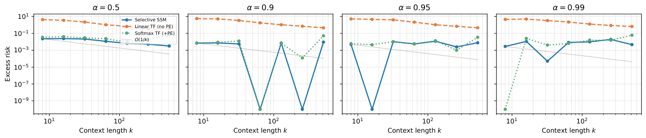
Figure 3.
Experiment II. Fixed-gain SSM plateaus at ; LinTF tracks the oracle rate; selective SSM partially recovers but plateaus at .
Figure 3.
Experiment II. Fixed-gain SSM plateaus at ; LinTF tracks the oracle rate; selective SSM partially recovers but plateaus at .
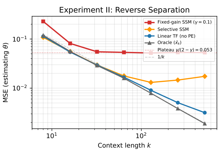
Figure 4.
Experiment III: Phase transition. Empirical (dots) versus theoretical (solid curve). The advantage collapses near the observability boundary and grows as .
Figure 4.
Experiment III: Phase transition. Empirical (dots) versus theoretical (solid curve). The advantage collapses near the observability boundary and grows as .
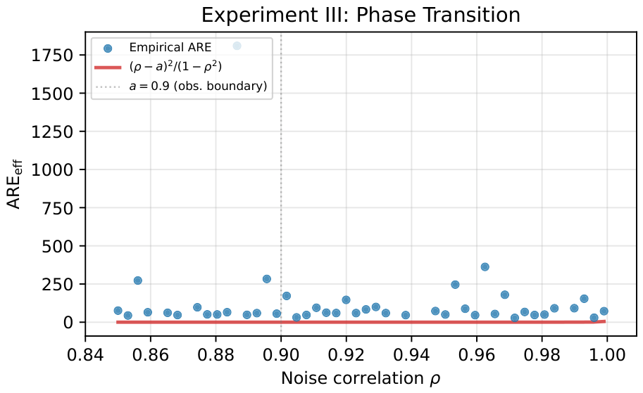
Figure 5.
(a) PE partially closes the gap: PI variants (a,b) suffer high excess risk; learned PE (d) nearly matches the SSM. (b) Mamba’s advantage is largest for sparse transitions ().
Figure 5.
(a) PE partially closes the gap: PI variants (a,b) suffer high excess risk; learned PE (d) nearly matches the SSM. (b) Mamba’s advantage is largest for sparse transitions ().
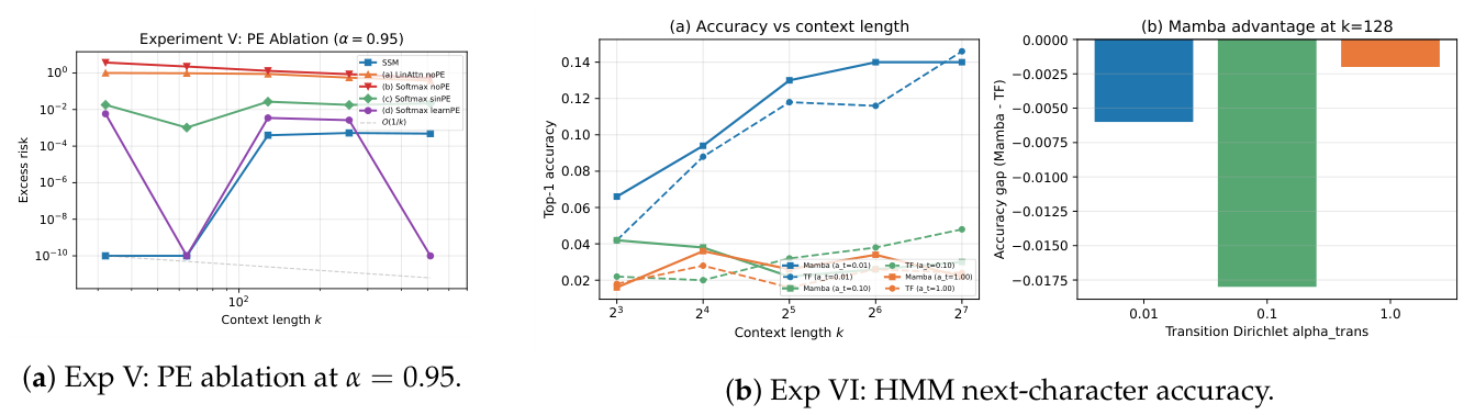
Figure 6.
Experiment VII: Structural chasm. MSE vs. sequence length on non-commutative product tracking. The SSM (4.7K params) outperforms all Transformers at despite having 10× fewer parameters than TF-4L (50.7K).
Figure 6.
Experiment VII: Structural chasm. MSE vs. sequence length on non-commutative product tracking. The SSM (4.7K params) outperforms all Transformers at despite having 10× fewer parameters than TF-4L (50.7K).
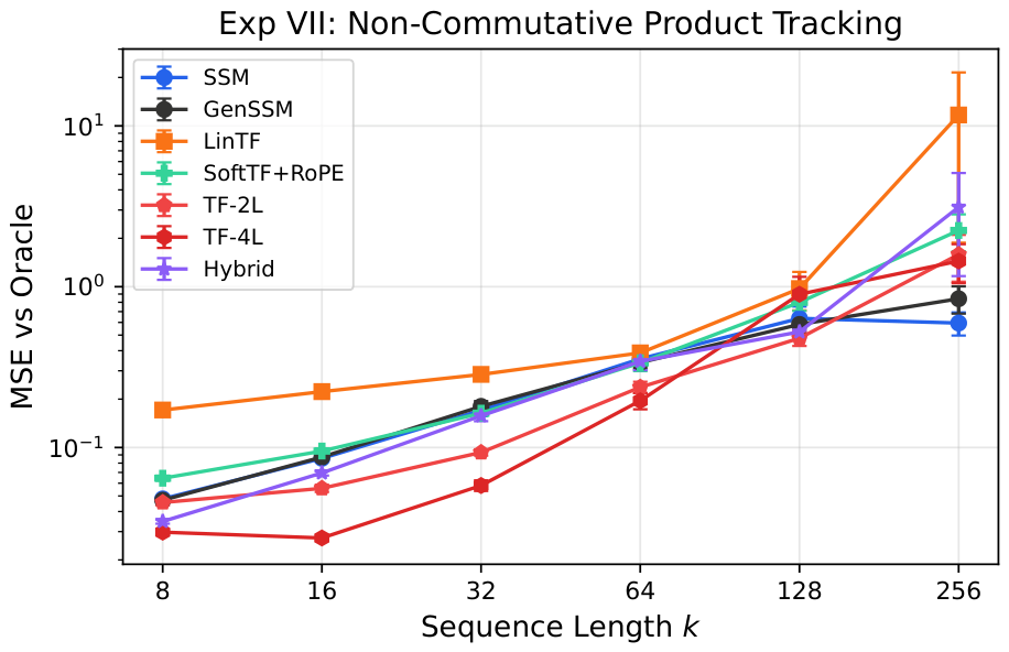
Table 1.
Empirical ARE at . LinTF values exceed the theoretical bound where measurable; is excluded because both models achieve near-oracle excess risk, making their ARE ratio numerically unstable ().
Table 1.
Empirical ARE at . LinTF values exceed the theoretical bound where measurable; is excluded because both models achieve near-oracle excess risk, making their ARE ratio numerically unstable ().
| 0.50 | 0.70 | 0.90 | 0.95 | 0.99 | |
|---|---|---|---|---|---|
| Theoretical ≥ | 1.33 | 1.96 | 5.26 | 10.26 | 50.25 |
| Linear Transf. (no PE) | 106.8 | — | 48.7 | 59.9 | 142.8 |
| Softmax Transf. (+PE) | 21.2 | — | 5.6 | 4.5 | 13.1 |
Table 2.
Experiment IV: Non-commutativity ablation. Empirical ARE at .
| Case (a): | Case (b): | |
|---|---|---|
| Linear Transf. (no PE) | 102.3 | 198.2 |
| Softmax Transf. (+PE) | 13.4 | |
| Predicted |
Table 3.
Experiment VII: MSE and extrapolation.†: trained at .
| Model | Params | MSE@ | MSE@ | MSE@ |
|---|---|---|---|---|
| SSM (Kron) | 4,760 | 0.356 | 0.594 | 0.808 |
| General SSM | 6,104 | 0.338 | 0.842 | 1.174 |
| LinTF (no PE) | 12,868 | 0.388 | 11.69 | — |
| SoftTF + RoPE | 12,868 | 0.336 | 2.24 | 2.00 |
| TF-2L + RoPE | 25,508 | 0.237 | 1.59 | 1.25 |
| TF-4L + RoPE | 50,660 | 0.195 | 1.44 | 1.60 |
| Hybrid | 20,472 | 0.344 | 3.13 | 2.19 |
Table 4.
Experiment VIII: Excess risk ratio on non-commutative product tracking. Ratio : SSM wins. At comparable parameter budgets (1L, K), the SSM wins across all PE types and the ratio increases with k—consistent with Theorem 1. At the SSM budget (2L), Transformers become competitive at but the advantage erodes at .
Table 4.
Experiment VIII: Excess risk ratio on non-commutative product tracking. Ratio : SSM wins. At comparable parameter budgets (1L, K), the SSM wins across all PE types and the ratio increases with k—consistent with Theorem 1. At the SSM budget (2L), Transformers become competitive at but the advantage erodes at .
| Model | Params | ||
|---|---|---|---|
| Comparable budget (≤ SSM’s 4.7K) | |||
| TF-1L (no PE) | 3,364 | 1.77 | 2.78 |
| TF-1L + Sinusoidal | 3,364 | 1.38 | 1.31 |
| TF-1L + RoPE | 3,364 | 1.64 | 2.64 |
| SSM budget | |||
| TF-2L (no PE) | 25,508 | 1.16 | 0.79 |
| TF-2L + RoPE | 25,508 | 0.89 | 1.15 |
Disclaimer/Publisher’s Note: The statements, opinions and data contained in all publications are solely those of the individual author(s) and contributor(s) and not of MDPI and/or the editor(s). MDPI and/or the editor(s) disclaim responsibility for any injury to people or property resulting from any ideas, methods, instructions or products referred to in the content. |
© 2026 by the authors. Licensee MDPI, Basel, Switzerland. This article is an open access article distributed under the terms and conditions of the Creative Commons Attribution (CC BY) license (http://creativecommons.org/licenses/by/4.0/).
Copyright: This open access article is published under a Creative Commons CC BY 4.0 license, which permit the free download, distribution, and reuse, provided that the author and preprint are cited in any reuse.


