

Submitted:
25 May 2026
Posted:
27 May 2026
You are already at the latest version
Abstract
In-context learning (ICL)—the ability of large language models to make predictions from a few input--output demonstrations without parameter updates---has become a defining capability of modern AI. Existing theoretical analyses either focus on pretraining dynamics, rely on intractable information-theoretic quantities, or provide only asymptotic characterizations, leaving a gap: no existing framework provides explicit generalization bounds with closed-form sample complexity formulas for ICL at inference time with a frozen pretrained model. We develop a comprehensive PAC-Bayes framework for inference-time ICL parameterized by two task-model quantities: the ambiguity A (zero-shot predictive entropy) and the saliency S (per-demonstration KL reduction rate). Under the linear attention model, both quantities admit closed-form expressions in architecture parameters and are exactly computable; for general Transformers, they can be estimated via Monte Carlo sampling. Our contributions span six directions: (1) a core generalization bound with O(√A/k) excess risk and closed-form sample complexity; (2) instantiation under linear attention yielding closed-form, architecture-dependent bounds; (3) a minimax lower bound proving the Θ(√A/k) rate is optimal; (4) Catoni fast-rate bounds achieving O(1/k) excess risk; (5) data-dependent priors via sample splitting that can eliminate the ambiguity term entirely; (6) Bernstein variance-adaptive bounds achieving fast rates through variance decay. We prove 20 theorems, 1 proposition, 5 lemmas, and 2 corollaries spanning these directions and validate key predictions through both synthetic Bayesian linear regression simulations and real in-context learning experiments with GPT-2 on NLP classification benchmarks (SST-2, AG News, SNLI).
Keywords:
in-context learning
; PAC-Bayes theory
; generalization bounds
; sample complexity
; minimax optimality
; linear attention
; transformer
1. Introduction
1.1. The Phenomenon of In-Context Learning
Large language models (LLMs) exhibit a remarkable ability: given a few input–output demonstrations in the prompt, they can make accurate predictions on new queries without updating any parameters [1]. This phenomenon, known as in-context learning (ICL), has profound practical implications and raises fundamental theoretical questions:
- Why does the number of required demonstrations vary dramatically across tasks (1–3 for sentiment analysis vs. 10+ for natural language inference)?
- Does there exist an optimal number of demonstrations, and can it be computed from model properties?
- What is the information-theoretic lower bound on the error—even with arbitrarily many demonstrations?
Despite extensive empirical study, these questions lack rigorous answers. Existing theoretical analyses fall into several categories—Bayesian inference interpretations, gradient descent analogies, algorithm selection frameworks, information-theoretic analyses, and asymptotic characterizations—none of which provides explicit, computable error bounds with sample complexity formulas for a frozen pretrained model at inference time.
1.2. Related Work
Bayesian implicit inference.
[2] model ICL as implicit Bayesian inference over a latent concept variable. While conceptually appealing, this view does not yield quantitative generalization guarantees or sample complexity formulas.
Gradient descent analogy.
Algorithm selection and stability.
Information-theoretic analysis.
[7] introduce conditional mutual information (e-CMI) tools to bound ICL excess risk without mixing-time assumptions. Their bounds depend on intractable e-CMI quantities rather than computable model properties, and they do not provide closed-form sample complexity, minimax lower bounds, fast rates, or architecture-dependent instantiations.
Bayesian model averaging and pretraining analysis.
[8] show that ICL implicitly implements Bayesian model averaging and establish an regret bound for perfectly pretrained ICL, where T is the prompt length. Their PAC-Bayes analysis targets the pretraining generalization error (as a function of the pretraining corpus size), not the inference-time generalization gap. In contrast, our framework analyzes the gap between population and empirical risk of a frozen model as a function of the number of demonstrations k, without assuming perfect pretraining. Moreover, their work does not provide minimax lower bounds, sample complexity formulas, data-dependent priors, or variance-adaptive bounds.
Asymptotic analysis of linear attention.
[9] derive sharp asymptotic characterizations of the ICL learning curve under linear attention in the proportional limit (), revealing phenomena such as double descent. Their results are exact but asymptotic, and they do not provide finite-sample PAC-Bayes bounds, sample complexity formulas, or minimax lower bounds. Our linear attention instantiation (Section 4) provides complementary finite-sample guarantees for the same model class.
Generalization of pretrained Transformers.
[10] prove a generalization bound of for Transformers trained on linear regression tasks, where S, T, n denote context window, sequence length, and number of tasks respectively. Their analysis focuses on the pretraining phase and the distinction between ICL and in-weight learning, whereas our framework targets the inference-time generalization of a frozen model and provides closed-form, architecture-dependent bounds parameterized by computable quantities.
PAC-Bayes theory.
The PAC-Bayes framework [11,12,13] bounds the generalization error of randomized predictors in terms of the KL divergence between a data-dependent posterior and a data-independent prior. Extensions include fast-rate bounds [13], Bernstein-type refinements [14,15], and data-dependent priors via sample splitting [16]. Our work brings this rich toolkit to bear on inference-time ICL, providing the first unified PAC-Bayes framework parameterized by computable task-model quantities.
1.3. Contributions
Our contributions are organized along six directions. To our knowledge, contributions (1), (3)–(6) are entirely new in the ICL literature; contribution (2) is the first to provide computable, closed-form architecture-dependent bounds for inference-time ICL (cf. Table 1).
- Core PAC-Bayes ICL framework (§Section 3): We establish generalization upper bounds parameterized by two computable quantities—ambiguity A and saliency S—that can be evaluated from the pretrained model without retraining. Unlike the conditional mutual information approach of [7], which yields non-computable bounds, and the Bayesian regret analysis of [8], which assumes a perfectly pretrained model and studies pretraining error, our bounds apply to any frozen pretrained Transformer at inference time with finitely many demonstrations. We further derive closed-form sample complexity, an information-theoretic lower bound, and a permutation variance bound (Theorems 2–6).
- Linear attention instantiation (§Section 4): Under a linear attention model, we derive closed-form expressions for A and S in terms of model dimension, prior variance, noise variance, and signal strength, yielding architecture-dependent bounds (Theorems 1–9). While [9] characterize linear attention ICL in an asymptotic () regime, our bounds are non-asymptotic and yield explicit sample complexity formulas.
- Minimax optimality (§Section 5.1): Using Le Cam’s two-point method and KL tensorization, we prove a matching lower bound, establishing that the rate is tight (Theorems 10–13). No prior work provides minimax lower bounds for ICL generalization.
- Catoni fast-rate bounds (§Section 5.2): With Catoni’s temperature-parameterized bound, we achieve excess risk when the empirical risk is small, reducing sample complexity from to (Theorems 14–16). This is the first fast-rate PAC-Bayes result in the ICL setting.
- Data-dependent priors (§Section 6.1): Via sample splitting, we construct informed priors that can eliminate the ambiguity term entirely (Theorems 17–19). No existing ICL analysis employs data-dependent priors.
- Bernstein variance-adaptive bounds (§Section 6.2): Exploiting low loss variance, we obtain a second path to fast rates through variance decay (Theorems 20–5). Variance-adaptive analysis for ICL has not appeared in prior work.
1.4. Paper Organization
Section 2 introduces the formal setup and key definitions. Section 3 presents the core framework. Section 4 develops the flagship linear attention instantiation. Section 5 establishes minimax optimality and fast rates. Section 6 presents the data-dependent prior and Bernstein extensions. Section 7 validates predictions via numerical simulations. Section 8 discusses implications, limitations, and open problems. Proofs are sketched in the main text; complete proofs appear in Appendices Appendix A–Appendix D.
2. Problem Setup and Key Definitions
2.1. ICL as a Statistical Learning Problem
Consider a pretrained model with frozen parameters . Given k in-context demonstrations drawn i.i.d. from a task distribution , the model produces a prediction for a new query . We formalize this within the PAC-Bayes framework by identifying:
- Prior P: the model’s zero-shot predictive distribution ;
- Posterior Q: the model’s predictive distribution after observing k demonstrations.
Definition 1
(Population and Empirical Risk). For a bounded loss function , define:
where both risks are computed with the model conditioned on the full demonstration set .
Remark 1
(Choice of empirical risk). We use the standard plug-in empirical risk (each example evaluated under the full context ) rather than a leave-one-out estimator. This is the natural form for PAC-Bayes analysis, where the bound requires the empirical risk and the posterior to be computed on the same sample. In ICL the model is frozen, so conditioning on introduces a mild optimistic bias (the prediction for benefits from having seen ). This bias is negligible for large k and can be corrected via a leave-one-out adjustment at the cost of a factor; we retain the standard form for compatibility with the PAC-Bayes theorem.
2.2. PAC-Bayes Preliminaries
Definition 2
(KL Divergence). For probability measures on a measurable space with ,
The fundamental tool throughout this paper is the McAllester PAC-Bayes bound:
Theorem 1
(McAllester [12]). Let P be a prior distribution over hypotheses fixed before observing data, Q any data-dependent posterior, a bounded loss, and k i.i.d. samples. Then for any , with probability at least :
This bound is derived from the Donsker–Varadhan variational inequality [17] combined with Hoeffding’s lemma [18]; see Appendix E for precise statements.
2.3. Ambiguity and Saliency
We parameterize the PAC-Bayes framework with two task-model quantities that are, in principle, computable from the pretrained model.
Definition 3
(Ambiguity). Theambiguityof task given model θ is the expected zero-shot predictive entropy:
Ambiguity serves as a natural upper bound on the KL divergence: .
Definition 4
(Saliency). Thesaliencyof model θ on task is the expected per-demonstration KL reduction:
Equivalently, S is the initial rate at which each demonstration reduces the posterior–prior KL divergence, measured in nats per demonstration. Under the linear attention model (Section 4), , which is the per-example Fisher information of the linear predictor along the task direction.
Definition 5
(Prior Quality Ratio). Theprior quality ratiois . A high indicates a model that is both uncertain (A large but finite) and responsive to demonstrations (S large), leading to efficient ICL.
2.4. KL Reduction: Rigorous Bound and Modeling Assumption
Our framework connects the posterior–prior KL divergence to the demonstration count k. We present a two-level treatment: (i) a rigorous KL bound for the Gaussian linear model, and (ii) a first-order modeling assumption for general architectures.
Proposition 1
(Exact KL Bound under Gaussian Model). Under the Bayesian linear regression model of Section 4 (prior , noise , isotropic inputs , signal strength s), the expected posterior–prior KL divergence after k demonstrations satisfies:
The bound is: (a) monotonically decreasing in k, (b) , and (c) as .
Proof
(Proof sketch). The posterior covariance satisfies (since and ). The Gaussian KL in closed form then yields (3). See Appendix B.2 for the full derivation. □
Corollary 1
(Linearization with Explicit Error). The exact bound and the linear approximation satisfy, for all :
The error is and is negligible when .
For general (non-Gaussian) architectures, we introduce a modeling assumption:
Assumption A1
(Approximate KL Reduction). For a general pretrained model , the posterior–prior KL divergence satisfies:
Remark 2.
For the Gaussian model, Assumption A1 follows from Proposition 1 up to the linearization error in Corollary 1. For general Transformer architectures, it remains a modeling hypothesis whose validity for softmax attention is an open question (Section 8).All results in Section 3, Section 4, Section 5 and Section 6 hold verbatim if is replaced by any monotone upper bound on , including the exact bound .
3. Core Generalization Framework
3.1. Upper Bounds
Theorem 2
(Basic ICL Generalization Bound). Let be a bounded loss, , and suppose with . Then for any , with probability at least :
Proof
(Proof sketch). Apply Theorem 1 directly. Since , monotonicity of the square root gives (4). The full proof is in Appendix A.1. □
Theorem 3
(Saliency-Enhanced ICL Bound). Under Assumption A1, with probability at least :
Proof
(Proof sketch). Replace the KL bound A in Theorem 2 with the tighter bound from Assumption A1. See Appendix A.2. □
3.2. Sample Complexity
Theorem 4
(Sample Complexity). Given a target accuracy and confidence , if the number of demonstrations satisfies
then .
Proof
(Proof sketch). From Theorem 2, condition (6) ensures . Combining with yields . The algebraic details are in Appendix A.3. □
Remark 3.
The formula exhibits the familiar scaling of PAC-Bayes sample complexity. The numerator captures task difficulty (ambiguity) and confidence requirements; the denominator captures the “improvability gap” between the target accuracy and the zero-shot baseline. High tasks (e.g., sentiment analysis) have small A, requiring few demonstrations; low tasks (e.g., natural language inference) have large A, requiring many more.

Table 2.
Predicted sample complexities for representative ICL tasks (). Values of A, S, are illustrative parameters chosen to span different difficulty regimes; Table 7 reports empirically measured values from GPT-2.
Table 2.
Predicted sample complexities for representative ICL tasks (). Values of A, S, are illustrative parameters chosen to span different difficulty regimes; Table 7 reports empirically measured values from GPT-2.
| Task analogue | A | S | |||
|---|---|---|---|---|---|
| Easy (SST-2–like) | 0.5 | 0.3 | 0.15 | 0.10 | 270 |
| Medium (AG News–like) | 2.0 | 0.4 | 0.30 | 0.15 | 237 |
| Hard (SNLI–like) | 5.0 | 0.2 | 0.45 | 0.20 | 567 |
3.3. Information-Theoretic Lower Bound
Theorem 5
(ICL Classification Lower Bound via Fano). Consider ICL for aclassificationtask with classes. Let denote the label entropy and suppose each demonstration provides at most S nats of mutual information about the label, so . Then the misclassification probability of any ICL estimator satisfies:
Proof
(Proof sketch). Apply Fano’s inequality [19]: . Substitute the bounds and . See Appendix A.4. □
Remark 4
(Scope of Theorem 5). Fano’s inequality applies to discrete label spaces. For the regression setting of Section 4, the minimax lower bound (Theorem 10) provides the analogous result via Le Cam’s method without requiring a discrete label space. The two bounds are complementary: Theorem 5 gives a lower bound on classification error; Theorem 10 gives a lower bound on excess risk for regression.
Theorem 5 shows that each demonstration contributes at most S nats of task-relevant information. Complete disambiguation (reducing to zero) requires demonstrations—an information-theoretic floor that no model, however powerful, can surpass.
3.4. Permutation Sensitivity
The ordering of in-context demonstrations can affect performance. We quantify this sensitivity using the Efron–Stein framework.
Theorem 6
(Permutation Variance Bound). Let σ denote a random permutation of k demonstrations. Under the bounded-differences condition (i.e., swapping any two demonstrations changes the loss by at most c), the variance of the ICL error over permutations satisfies:
Proof
(Proof sketch). The Efron–Stein inequality [20] gives . Substituting and simplifying yields . See Appendix A.5. □
The decay rate implies that ordering sensitivity vanishes for large k. High-saliency tasks are more order-sensitive—a double-edged sword of saliency: responsiveness accelerates learning but increases sensitivity to demonstration arrangement.
4. Linear Attention: Architecture-Dependent Bounds
The bounds in Section 3 are expressed in terms of the abstract quantities A and S. In this section, we instantiate these for a concrete architecture—linear attention—and obtain bounds that depend directly on model parameters.
4.1. Linear Attention as Bayesian Linear Regression
Following [4] and [21], we model a single-layer linear attention head performing ICL on d-dimensional inputs as implicit Bayesian linear regression. The generative model is:
- Task parameter: ;
- Observations: , with ;
- Signal strength: a parameter measuring the effective task signal captured by the attention head.
Under this model, the posterior after k demonstrations is Gaussian with a closed-form KL divergence to the prior, enabling exact computation of A and S.
4.2. Closed-Form Ambiguity and Saliency
Definition 6
(Effective Ambiguity). Under the linear attention model with dimension d, prior variance , and noise variance :
Definition 7
(Effective Saliency). Under the same model with signal strength s:
Both and are strictly positive for all valid model parameters, since , , , , and for .
4.3. Simplified Bounds via Classical Inequalities
Lemma 1
(Ambiguity Upper Bound). For all valid parameters:
Proof.
Apply for with , then multiply by . □
Lemma 2
(Saliency Upper Bound). When : .
Proof
(Proof sketch). Since , we have . See Appendix B.1. □
The bound (9) replaces the logarithmic expression with a simpler rational one, making sample complexity formulas more transparent.
4.4. The Saturation Phenomenon
Lemma 3
(KL Saturation). When , and the KL complexity term vanishes entirely.
Theorem 7
(Post-Saturation Bound). For , with probability at least :
Proof
(Proof sketch). By Theorem 3, the KL term in Assumption A1 equals zero. Apply Theorem 1 with to obtain (10), the tightest possible PAC-Bayes bound where only the sub-Gaussian concentration term remains. See Appendix B.3. □
The saturation point represents a phase transition: below it, each demonstration contributes nats of information, tightening the bound; above it, the KL term has been fully absorbed, and only the confidence penalty persists. Under the linear attention model:
which is computable from the model architecture.
4.5. End-to-End Architecture-Dependent Bound
Theorem 8
(Linear Attention ICL Bound). Under the linear attention model with parameters , with probability at least :
where and .
Proof
(Proof sketch). The Bayesian conjugacy structure of the Gaussian model implies that the posterior KL after k demonstrations satisfies Assumption A1 with and . Apply Theorem 3 with these values. See Appendix B.4. □
4.6. Simplified Sample Complexity
Theorem 9
(Architecture-Dependent Sample Complexity). Under the linear attention model, if
then .
Proof
(Proof sketch). Apply Theorem 1 to weaken in Theorem 4, replacing the logarithmic term with the simpler rational upper bound. See Appendix B.5. □
Corollary 2.
The required number of demonstrations scales as , where is the signal-to-noise ratio. Reducing d (via projection or compression) or improving SNR (via better pretraining) directly reduces the demonstration requirement.
Table 3.
Architecture-dependent sample complexities for , .
| d | SNR | ||||
|---|---|---|---|---|---|
| 5 | 1.0 | 1.0 | 1.73 | 1.0 | 238 |
| 10 | 1.0 | 1.0 | 3.47 | 1.0 | 325 |
| 10 | 1.0 | 0.5 | 5.49 | 2.0 | 426 |
| 20 | 0.5 | 1.0 | 2.23 | 0.5 | 263 |
| 50 | 1.0 | 1.0 | 17.33 | 1.0 | 1018 |
5. Minimax Optimality and Fast Rates
5.1. Minimax Lower Bounds
Having established an upper bound, a natural question is whether this rate is optimal. We answer affirmatively using Le Cam’s two-point method.
Theorem 10
(Minimax Lower Bound). Consider the class of ICL tasks with bounded loss and ambiguity at most A. For any ICL estimator and any , there exist two tasks with such that the maximum risk over the pair satisfies:
Proof
(Proof sketch) Concrete construction.. Let denote the first standard basis vector in . Define two Gaussian regression tasks:
- : , ;
- : , ;
with risk gap and per-sample KL divergence . Both tasks satisfy since the zero-shot prediction is the same (zero mean) with entropy determined by . By KL tensorization, . Le Cam’s two-point method [22] gives . Substituting and simplifying yields (13). See Appendix C.1 for the complete proof. □
Theorem 11
(Simplified Minimax Lower Bound). When , the lower bound simplifies to:
Proof
(Proof sketch). When , we have , so . Multiply the factor of by to get . See Appendix C.2. □
Theorem 12
(Rate Optimality). The ICL generalization rate is :
- Upper bound: (Theorem 2);
- Lower bound: (Theorem 11).
Both bounds match up to universal constants, establishing rate optimality.
Theorem 13
(Saturation-Regime Lower Bound). After saturation (), an information-theoretic cost persists:
This shows that even after the KL complexity term vanishes, a confidence-based irreducible term remains.
5.2. Catoni Fast-Rate Bounds
The McAllester bound (Theorem 1) yields an excess risk. Using Catoni’s temperature-parameterized PAC-Bayes bound [13], we can achieve when the empirical risk is small.
Theorem 14
(Catoni ICL Bound). Setting the temperature parameter in Catoni’s bound and using :
The excess risk is when is small.
Proof
(Proof sketch). Catoni’s bound [13] with parameter gives
Setting : the coefficient becomes and . Weakening yields (16). See Appendix C.3. □
Theorem 15
(Fast-Rate Sample Complexity). If and , then . Since , an explicit sufficient condition is (obtained by solving the implicit inequality via where ). The sample complexity is —a quadratic improvement over the McAllester-based .
Proof
(Proof sketch). Each of the two terms in (16) contributes at most , and . See Appendix C.4. □
Lemma 4
(Catoni Dominates McAllester for Large k). Let . An explicit sufficient condition for the Catoni excess risk to be strictly smaller than the McAllester excess risk is (since for , giving ).
Proof.
Under , squaring both sides of gives , i.e., , which holds by hypothesis. □
Theorem 16
(Fast Rate with Zero Empirical Risk). Under perfect empirical fit ():
This is the purest form of the fast rate and is particularly relevant for ICL, where well-pretrained models typically achieve near-zero empirical risk on in-context demonstrations.
6. Extensions
6.1. Data-Dependent Priors via Sample Splitting
Standard PAC-Bayes requires data-independent priors, but in ICL the zero-shot distribution implicitly depends on pretraining data. The split-sample technique [16] resolves this by partitioning k demonstrations into (for constructing an informed prior) and (for evaluation).
Theorem 17
(Information Gain Reduces KL). Using demonstrations to build an informed prior, the effective KL satisfies:
where is the per-demonstration information gain.
Proof
(Proof sketch). Each of the demonstrations contributes nats toward resolving the task ambiguity, reducing the remaining KL from A to . The ensures non-negativity. See Appendix D.1. □
Theorem 18
(Data-Dependent ICL Bound). With split-sample PAC-Bayes, the population risk satisfies:
Proof
(Proof sketch). Apply the split-sample PAC-Bayes bound [16] with the reduced KL from Theorem 17, then weaken the KL term via monotonicity. See Appendix D.1. □
Theorem 19
(Fully Informed Prior). When (the prior is “fully informed”):
The ambiguity term vanishes entirely.
Proof
(Proof sketch). When , we have . Substitute into (19) and simplify. See Appendix D.1. □
The split bound’s numerator is always at most the standard bound’s, since .
The optimal split ratio depends on the information gain rate. When is large, a small suffices to eliminate ambiguity, leaving most demonstrations for evaluation.
6.2. Bernstein Variance-Adaptive Bounds
When the model is highly confident (low loss variance), the Hoeffding-based bounds in Section 3 are loose. Bernstein-type PAC-Bayes bounds [14,15] exploit low variance.
Theorem 20
(Bernstein ICL Bound). Let V denote the loss variance and . Under :
Proof
(Proof sketch). Apply the Bernstein PAC-Bayes bound [15] and weaken in both the (variance) term and the linear (remainder) term via monotonicity. See Appendix D.2. □
The bound (21) has two terms: a “variance term” and a “remainder term” . When V is small, the variance term becomes negligible, and the remainder term dominates at rate .
Theorem 21
(Variance Decay ⇒ Fast Rate). Under variance decay , the Bernstein bound becomes:
Since ,both terms are , yielding a fast rate.
Proof
(Proof sketch). Substitute into the variance term of (21). The numerator factor becomes , and dividing by k gives . See Appendix D.2. □
Lemma 5
(Bernstein Sqrt Term Absorption). When (where ): . The variance term is absorbed into the scale.
Proof
(Proof sketch). We show by substituting : the left side is at most , which equals the right side. Apply monotonicity and . See Appendix D.2. □
Table 4.
Comparison of the three PAC-Bayes bound families for ICL.
| Bound Family | Excess Risk Rate | Key Assumption | Best Regime |
|---|---|---|---|
| McAllester (Thm 2) | General | ||
| Catoni (Thm 14) | small | Large k, low emp. risk | |
| Bernstein (Thm 20) | Variance V small | Confident model |
Theorem 21 provides a second path to fast rates, complementing Catoni (Section 5.2). The Catoni path requires low empirical risk; the Bernstein path requires low variance. Both conditions are natural for well-pretrained models: on tasks where the model is well-matched, empirical risk is near zero and the model is confident (low variance).
7. Experimental Validation
We validate the key theoretical predictions in two complementary settings: (i) synthetic Bayesian linear regression tasks that exactly match the linear attention model of Section 4 (Experiments 1–4), and (ii) real in-context learning with GPT-2 on NLP classification benchmarks where model assumptions may not hold (Experiments 5–7). Synthetic experiments use independent trials and confidence level .
7.1. Setup
Data generation.
For each trial, we sample a task parameter and k input–output pairs with and , . The ICL prediction is the Bayesian posterior mean after k demonstrations. The loss is the squared error clipped to : .
Configurations.
We consider three configurations that span different effective ambiguity and saliency regimes, with signal strength parameter s controlling the effective saliency:
| Config | d | s | |||||
| A | 5 | 1.0 | 1.0 | 0.15 | 1.73 | 0.375 | 5 |
| B | 10 | 1.0 | 1.0 | 0.10 | 3.47 | 0.500 | 7 |
| C | 10 | 1.0 | 0.5 | 0.10 | 5.49 | 0.500 | 11 |
7.2. Experiment 1: Generalization Bound Tightness
For each configuration and each k, we compute the average population risk and training risk over N trials, and compare the generalization gap against the saliency-enhanced bound (Theorem 3).
Table 5 reports results for Config C (, , ), which has the largest effective ambiguity.
Observations.
The bound holds as a high-probability statement over individual trials. When examining the average gap, we observe that at the mean gap exceeds the bound. This is not a bound violation: the PAC-Bayes bound guarantees with probability , and the empirical violation rate over trials is , consistent with the theoretical guarantee. Before saturation (), the bound decreases rapidly due to the term; after saturation, only the confidence term remains. At , the bound exceeds 1, making it vacuous (for ); this is typical of PAC-Bayes bounds at very small sample sizes [23]. Results for Configs A and B exhibit the same qualitative pattern.
7.3. Experiment 2: Risk Scaling
We track population risk as a function of k for Config B (, ) over the range . Figure 1 shows the convergence behavior.
Observations.
The population risk decreases monotonically with k, from at to at . The increasing ratio reflects the fact that the total risk includes an irreducible noise component -dependent Bayes risk that does not vanish. The theoretical bound remains valid throughout, converging toward the empirical risk as k grows. This confirms that the rate correctly captures the learnable component of the risk.
7.4. Experiment 3: Saturation Point Verification
Theorems 3–7 predict a phase transition at . We verify this using Config C (), which has the largest saturation point. Figure 2 shows the KL complexity term and bound gap before and after .
Observations.
The KL complexity term decreases linearly from at to 0 at and remains zero thereafter, exactly as predicted. The bound gap drops rapidly in the pre-saturation regime (from to ) due to the combined effect of KL reduction and decay, then transitions to the slower -only rate post-saturation. The empirical risk mirrors this transition: the risk decreases by units over to 11 (pre-saturation), but only by units over to 50 (post-saturation), despite the latter interval being wider. This confirms the phase transition at .
7.5. Experiment 4: McAllester vs. Catoni Crossover
We compare the McAllester bound (Theorem 2) and the Catoni bound (Theorem 14) as functions of k for Config B with (the perfect empirical fit regime most relevant for well-pretrained models). Figure 3 shows the two bound curves.
Observations.
For small k, the Catoni bound is substantially looser due to its multiplicative constant of 2 (cf. Theorem 14). As k increases, the scaling of the Catoni excess term dominates the McAllester term. The crossover occurs at , after which Catoni provides strictly tighter guarantees. Theorem 4 predicts the crossover condition where ; at , , giving , so the condition is indeed satisfied. The gap widens dramatically for large k: at , the Catoni bound () is approximately half the McAllester bound (), confirming the practical relevance of fast rates.
With , the crossover shifts to ; with , the crossover exceeds , illustrating the sensitivity of the fast-rate advantage to the empirical risk level.
The preceding experiments validate the framework in a controlled setting where all theoretical quantities are known in closed form. We now turn to experiments with a real pretrained Transformer—GPT-2 (124M parameters) [24]—on genuine NLP classification tasks, where Assumption A1 may not hold exactly and quantities A and S must be estimated empirically.
7.6. Real Transformer Setup
Model and protocol.
We use GPT-2 [24] (124M parameters, 12 layers, 768 hidden dimensions) with softmax attention and positional encoding—the full architecture, not the linear attention approximation of Section 4. For each task, we format ICL as: k labeled demonstrations followed by an unlabeled query, all concatenated in the prompt. The model’s prediction is obtained via restricted softmax: we extract the logits at the last token position for the valid label tokens only (each verified to be a single BPE token) and apply softmax to obtain a probability distribution over labels. The loss is the 0–1 classification error: .
Tasks.
Estimation protocol.
For each task, we use 100 test examples and 500 demonstration candidates. Ambiguity is estimated as the mean zero-shot entropy: . KL divergence is estimated as the mean averaged over test examples and random demonstration draws. Saliency is estimated from the empirical risk curve: , where is the smallest k achieving of the maximum risk improvement.
7.7. Experiment 5: Bound Verification with GPT-2
Table 6 reports the PAC-Bayes bound evaluation on SST-2 with GPT-2. The estimated ambiguity is nats (near the maximum for binary classification), reflecting that GPT-2’s zero-shot label distribution is nearly uniform for sentiment under our prompt format.
Observations.
The PAC-Bayes bound holds for all k values: throughout. The bound gaps decrease from () to () at the rate predicted by Theorem 2, and the measured-KL bound is consistently tighter than the A-only bound (6– improvement), confirming that using the empirical KL rather than the ambiguity upper bound yields tighter guarantees. The absolute bounds remain vacuous () because GPT-2’s empirical risk on its own demonstrations is high (–), reflecting that this small model does not reliably “copy” label patterns from context. The high is itself informative: the bound correctly diagnoses poor ICL by producing large values. As the model quality improves (larger models, lower ), the bounds become progressively tighter.
7.8. Experiment 6: KL Behavior Under Softmax Attention
Assumption A1 posits that decreases linearly with k as . Figure 4 tests this prediction by comparing the measured against the linear model.
Observations.
The measured KL divergence is approximately constant across k (– nats), in contrast to the linear decrease predicted by Assumption A1. This confirms that the linear KL reduction is a modeling hypothesis specific to the Gaussian model, not a property of softmax Transformers. Crucially, the measured-KL bound (Theorem 2) remains valid throughout, as guaranteed by the theory. The saliency-enhanced bound (which assumes linear KL decay) is also valid here because the saturation point means for all tested k, reducing the saliency bound to the same form. As noted in Remark 2, all bounds hold verbatim when is replaced by any upper bound on ; the constant KL profile observed here satisfies for all k, so the A-only bound (which requires only ) is always valid.
7.9. Experiment 7: Multi-Task Complexity Estimation
Table 7 compares the estimated , , and predicted across three tasks of varying difficulty.
Observations.
The results reveal a clear saliency ordering: SST-2 has the highest estimated saliency () and shows the largest ICL improvement (), while SNLI has the lowest saliency () and negligible improvement (). This ordering—easy sentiment task responds most to demonstrations, hard inference task responds least—matches the qualitative predictions of the framework.
The AG News result is instructive: despite having the highest ambiguity (), the model’s performance degrades with demonstrations (). This occurs because GPT-2’s zero-shot topic prediction is already reasonable (70% accuracy), but ICL with the prompt format used here introduces conflicting signals that confuse the model. The framework correctly captures this failure: the low and high predict that many demonstrations are needed (), and indeed performance has not converged within the window. This demonstrates that the parameterization provides meaningful diagnostic information even when ICL fails.
Compared to the hypothetical values in Table 2, the measured ambiguities (– nats) are of the same order as the assumed values (– nats), though the measured range is compressed because GPT-2’s label-space entropy is limited by the number of classes. The saliency estimates (–) are substantially smaller than the assumed values (–), reflecting GPT-2’s limited ICL capacity on these tasks. Larger models with stronger ICL abilities would exhibit higher , yielding tighter bounds and smaller .
8. Discussion
8.1. Implications for Model Design
The sample complexity formula from Theorem 9 and Corollary 2 has direct design implications:
- Dimensionality reduction: Reducing the effective dimension d (via projection heads or attention bottlenecks) linearly reduces the demonstration requirement.
- Pretraining quality: Improving the SNR through better pretraining data directly improves ICL sample efficiency.
- Diminishing returns: Beyond the saturation point , additional demonstrations provide only improvement—a much slower rate.
8.2. ICL vs. Fine-Tuning
Fine-tuning a model on k examples yields excess risk scaling as , where is the effective parameter count. ICL achieves where A is typically much smaller than , since ICL operates in the model’s “natural” predictive space rather than the full parameter space. This explains why ICL can outperform fine-tuning with very few demonstrations when the model’s prior is well-matched to the task. The crossover occurs when k is large enough that fine-tuning’s greater flexibility outweighs ICL’s lower effective complexity.
8.3. ICL vs. Standard Machine Learning
Our framework reveals that ICL and standard supervised learning differ not merely in constants but in the objects the PAC-Bayes machinery operates on. In standard PAC-Bayes theory, the posterior Q and prior P live over model parameters; measures parameter deviation, and sample complexity scales as . In ICL, no parameters are updated: Q is the conditional predictive distribution of a frozen model, P is its zero-shot prediction encoding pretraining knowledge, and equals the ambiguity A—a measure of prediction shift, not parameter deviation. Consequently, sample complexity (Theorem 4) is decoupled from model size: a 175B-parameter model may have for a well-matched task. Moreover, ICL exhibits hard saturation at (Theorem 3), with no analog in standard learning where more data always helps. Table 8 summarizes these structural contrasts.
8.4. Limitations
Several limitations warrant discussion:
- 1.
- KL reduction assumption: Proposition 1 provides a rigorous KL bound for the Gaussian model with explicit linearization error (Corollary 1). For general Transformer architectures, Assumption A1 remains a modeling hypothesis. Experiment 6 confirms that softmax attention exhibits approximately constant (not linearly decreasing) KL divergence across k, but the core PAC-Bayes bound (Theorem 2) remains valid with the measured KL values.
- 2.
- Bounded loss: The requirement excludes unbounded losses such as cross-entropy on raw logits. Extending to sub-Gaussian losses is a natural direction.
- 3.
- 4.
- Computability of A and S: Under the linear attention model, A and S are exactly computable. For general LLMs, requires integration over the (unknown) input distribution; in practice, A and S must be estimated from a held-out sample, introducing estimation error not captured by the bound.
- 5.
- Linear attention model: While providing clean closed-form results, the linear attention model omits softmax nonlinearity, multi-head interaction, and positional encoding effects.
- 6.
- i.i.d. demonstrations: The framework assumes demonstrations are i.i.d., which may not hold in conversational or curriculum-based ICL settings.
8.5. Open Questions
- 1.
- Can the KL linear reduction be extended to softmax attention via local linearization around the softmax operating point?
- 2.
- How do multi-task ICL bounds look when tasks share ambiguity and saliency structure?
- 3.
- Can the permutation variance bound (Theorem 6) be tightened using task-specific ordering heuristics?
- 4.
- Does a data-dependent saliency that decays with k lead to tighter bounds than the constant-S assumption?
- 5.
- What are the computational-statistical tradeoffs when the attention capacity limits the effective number of demonstrations the model can process?
9. Conclusions
We have developed a comprehensive PAC-Bayes framework for in-context learning, comprising 28 formal results (20 theorems, 1 proposition, 5 lemmas, and 2 corollaries) across six directions: core generalization bounds, architecture-dependent instantiation under linear attention, minimax lower bounds establishing rate optimality, Catoni fast-rate bounds, data-dependent priors via sample splitting, and Bernstein variance-adaptive bounds.
The framework is parameterized by two computable quantities—ambiguity A and saliency S—that together determine the ICL generalization rate , the saturation point , and the sample complexity . Under the linear attention model, these quantities acquire closed-form expressions in the model architecture parameters, yielding fully explicit, computable bounds.
Our results provide a unified theoretical explanation for key empirical observations about ICL: why different tasks require different numbers of demonstrations, why performance improves rapidly and then saturates, and why well-pretrained models are more sample-efficient. Experiments with GPT-2 on SST-2, AG News, and SNLI confirm that the PAC-Bayes bounds hold for real softmax Transformers, that the measured KL divergence deviates from the linear model but the framework remains valid with empirical KL values, and that the parameterization provides meaningful diagnostic information across tasks. The framework opens several directions for future work, including scaling the empirical validation to larger models, extensions to multi-task settings, and non-i.i.d. demonstration sequences.
Appendix A. Proofs for Core Framework (Section 3)
Appendix A.1. Proof of Theorem 2 (Basic ICL Bound)
Proof.
By Theorem 1 (McAllester), with probability at least :
Since and is monotonically increasing, we have
Combining:
□
Appendix A.2. Proof of Theorem 3 (Saliency-Enhanced Bound)
Proof.
By Assumption A1, . Apply Theorem 1:
where the second inequality uses monotonicity of and . □
Appendix A.3. Proof of Theorem 4 (Sample Complexity)
Proof.
Let and . From the hypothesis , we derive:
Since is monotonically increasing and both sides of (A1) are non-negative:
By Theorem 2 and :
□
Appendix A.4. Proof of Theorem 5 (ICL Lower Bound)
Proof.
By Fano’s inequality [19], for any estimator of a discrete random variable Y with observed through channel X:
Substituting and :
The inequality (since ) ensures the division is valid and preserves the direction. □
Appendix A.5. Proof of Theorem 6 (Permutation Variance)
Proof.
The Efron–Stein inequality [20] applied to the loss function of a random permutation gives:
where c is the bounded-differences constant (maximum change from a single transposition). Substituting the hypothesis :
□
Appendix B. Proofs for Linear Attention (Section 4)
Appendix B.1. Proofs of Theorems 1 and 2
Proof
(Proof of Theorem 1). Using the classical inequality for with :
□
Proof
(Proof of Theorem 2). Since , we have . Therefore:
□
Appendix B.2. Proof of Proposition 1 and Corollary 1
Proof
(Proof of Proposition 1). Under the Bayesian linear regression model, the posterior after k observations with is:
Using the Gaussian KL closed form (Appendix E, item 7) and taking expectations over , the key step is the posterior covariance bound. Since and the effective signal strength is s per example, we obtain the deterministic bound . The Gaussian KL with diagonal covariances yields:
where the last inequality uses after taking expectations and applying Jensen’s inequality. Properties (a)–(c) follow directly: (a) monotonicity since is decreasing in k; (b) ; (c) as . □
Proof
(Proof of Corollary 1). The first inequality is immediate from monotonicity (property (a)). For the linearization error, note satisfies and . By Taylor’s theorem with integral remainder: . Since , the stated bound follows. □
Appendix B.3. Proofs of Theorems 3–7
Proof
(Proof of Theorem 3). By definition of max, if (i.e., ), then . □
Proof
(Proof of Theorem 7). By Theorem 3, the KL bound equals zero. Apply Theorem 1 with :
□
Appendix B.4. Proof of Theorem 8 (Linear Attention ICL Bound)
Proof.
The Bayesian conjugacy structure (Appendix B.2) implies that the posterior KL satisfies Assumption A1 with and . Apply Theorem 3 with these values to obtain:
□
Appendix B.5. Proof of Theorem 9
Proof.
By Theorem 1, . Since is monotone:
The condition (12) ensures this quantity is at most . Apply Theorem 4 to conclude . □
Appendix C. Proofs for Minimax Optimality and Fast Rates (Section 5)
Appendix C.1. Proof of Theorem 10 (Minimax Lower Bound)
Proof.
We use Le Cam’s two-point method. Construct two ICL tasks satisfying:
- 1.
- Risk gap: (the difference in optimal risk between the two tasks).
- 2.
- Per-sample KL divergence: .
By Le Cam’s inequality [22], the maximum risk of any estimator over satisfies:
By the KL tensorization property (for i.i.d. observations):
Substituting:
□
Appendix C.2. Proof of Theorem 11
Proof.
When : , so , hence . From Theorem 10:
□
Appendix C.3. Proof of Theorem 14 (Catoni ICL Bound)
Proof.
Catoni’s PAC-Bayes bound [13] with temperature states:
Setting :
- Coefficient: .
- Denominator: .
Weakening :
Therefore:
□
Appendix C.4. Proof of Theorem 15
Proof.
Let . By hypothesis, and . From Theorem 14:
□
Appendix C.5. Proof of Theorem 4
Proof.
We need to show when . Squaring both sides (both are non-negative since and ):
The inequality is equivalent to , i.e., . This holds by hypothesis. □
Appendix D. Proofs for Extensions (Section 6)
Appendix D.1. Proofs for Data-Dependent Priors
Proof
(Proof of Theorem 17). Each of the demonstrations contributes nats toward resolving the task. The remaining KL divergence is at most . Since KL divergence is non-negative:
□
Proof
(Proof of Theorem 18). Apply the split-sample PAC-Bayes bound [16] on the evaluation examples with the data-dependent prior :
By Theorem 17, . Monotonicity of :
□
Proof
(Proof of Theorem 19). When , we have , so . Substituting into Theorem 18:
□
Appendix D.2. Proofs for Bernstein Variance-Adaptive Bounds
Proof
(Proof of Theorem 20). The Bernstein PAC-Bayes bound [15] states:
where . Since , both the term and the linear term are monotonically increasing in KL. Therefore:
Combining with the Bernstein bound yields (21). □
Proof
(Proof of Theorem 21). Let . Under , the numerator of the variance term becomes:
Dividing by k (the denominator inside from Theorem 20):
By monotonicity:
Both the variance term and the remainder term are . □
Proof
(Proof of Theorem 5). We show , which implies by monotonicity.
Since :
Taking square roots of both sides (both are non-negative):
□
Appendix E. Classical Results Used
For completeness, we state the classical results invoked as foundational tools. We do not re-prove these well-established results; references to original proofs are provided.
- 1.
- KL non-negativity (Gibbs inequality): whenever . See [29], Theorem 2.6.3.
- 2.
- Hoeffding’s lemma [18]: If X satisfies and , then .
- 3.
- Donsker–Varadhan variational inequality [17]: For any measurable f and : .
- 4.
- McAllester’s PAC-Bayes bound [12]: See Theorem 1.
- 5.
- Fano’s inequality [19]: .
- 6.
- Bounded differences (McDiarmid’s inequality) [30]: Variance bound via Efron–Stein; see Theorem 6.
- 7.
- Gaussian KL closed form: For and : . See [29].
- 8.
- Catoni’s PAC-Bayes bound [13]: Temperature-parameterized bound with .
- 9.
- Le Cam’s two-point method [22]: .
- 10.
- KL tensorization: for product distributions.
- 11.
- Split-sample PAC-Bayes [16]: PAC-Bayes bound with data-dependent priors via sample splitting.
- 12.
- Bernstein PAC-Bayes [15]: Variance-aware PAC-Bayes bound with structure.
Appendix F. Simulation Details
Appendix F.1. Pseudocode
| Algorithm 1:Bayesian Linear Regression ICL Simulation |
|
Appendix F.2. Hyperparameters
Table A1.
Simulation hyperparameters.
| Parameter | Value |
|---|---|
| Dimension d | |
| Prior variance | 1.0 |
| Noise variance | |
| Signal strength s | |
| Max demonstrations | 200 (Exp. 2), 50 (others) |
| Number of trials N | 2000 |
| Confidence parameter | 0.05 |
| Random seed | 42 |
Appendix F.3. Reproducibility
All simulations are implemented in Python 3.13 using NumPy 2.3. The complete simulation script (run_simulations.py) reproduces all tables in Section 7 with a single execution. Computation time is approximately 10 minutes on a standard workstation.
References
- Brown, T.B.; Mann, B.; Ryder, N.; Subbiah, M.; Kaplan, J.; Dhariwal, P.; Neelakantan, A.; Shyam, P.; Sastry, G.; Askell, A.; et al. Language models are few-shot learners. Adv. Neural Inf. Process. Syst. 2020, Vol. 33, 1877–1901. [Google Scholar]
- Xie, S.M.; Raghunathan, A.; Liang, P.; Ma, T. An explanation of in-context learning as implicit Bayesian inference. International Conference on Learning Representations, 2022. [Google Scholar]
- von Oswald, J.; Niklasson, E.; Randazzo, E.; Sacramento, J.; Mordvintsev, A.; Zhmoginov, A.; Vladymyrov, M. Transformers learn in-context by gradient descent. International Conference on Machine Learning, 2023; pp. 35151–35174. [Google Scholar]
- Akyürek, E.; Schuurmans, D.; Andreas, J.; Ma, T.; Zhou, D. What learning algorithm is in-context learning? Investigations with linear models. International Conference on Learning Representations, 2023. [Google Scholar]
- Bai, Y.; Chen, F.; Wang, H.; Xiong, C.; Mei, S. Transformers as statisticians: Provable in-context learning with in-context algorithm selection. Adv. Neural Inf. Process. Syst. 2023, Vol. 36. [Google Scholar]
- Li, Y.; Ildiz, M.E.; Papailiopoulos, D.; Oymak, S. Transformers as algorithms: Generalization and stability in in-context learning. International Conference on Machine Learning, 2023. [Google Scholar]
- Jeon, H.J.; Lee, J.D.; Lei, Q.; Van Roy, B. An information-theoretic analysis of in-context learning. International Conference on Machine Learning, 2024. [Google Scholar]
- Zhang, R.; Frei, S.; Bartlett, P.L. What and how does in-context learning learn? Bayesian model averaging, parameterization, and generalization. International Conference on Artificial Intelligence and Statistics, 2025. [Google Scholar]
- Lu, Y.M.; Letey, M.I.; Zavatone-Veth, J.A.; Maiti, A.; Pehlevan, C. Asymptotic theory of in-context learning by linear attention. Proc. Natl. Acad. Sci. 2025, 122. [Google Scholar] [CrossRef] [PubMed]
- Liu, S.; Cai, Z.; Chen, G.; Li, X. Towards better understanding of in-context learning ability from in-context uncertainty quantification. Transactions on Machine Learning Research, 2025. [Google Scholar]
- McAllester, D.A. PAC-Bayesian model averaging. In Proceedings of the Twelfth Annual Conference on Computational Learning Theory, 1999; pp. 164–170. [Google Scholar]
- McAllester, D. PAC-Bayesian stochastic model selection. Mach. Learn. 2003, 51, 5–21. [Google Scholar] [CrossRef]
- Catoni, O. PAC-Bayesian Supervised Classification: The Thermodynamics of Statistical Learning. In Institute of Mathematical Statistics Lecture Notes – Monograph Series; Institute of Mathematical Statistics, 2007; Vol. 56. [Google Scholar]
- Seldin, Y.; Laviolette, F.; Cesa-Bianchi, N.; Shawe-Taylor, J.; Auer, P. PAC-Bayesian inequalities for martingales. IEEE Trans. Inf. Theory 2012, 58, 7086–7093. [Google Scholar] [CrossRef]
- Tolstikhin, I.O.; Seldin, Y. PAC-Bayes-Empirical-Bernstein inequality. Adv. Neural Inf. Process. Syst. 2013, Vol. 26. [Google Scholar]
- Lever, G.; Laviolette, F.; Shawe-Taylor, J. Tighter PAC-Bayes bounds through distribution-dependent priors. Theor. Comput. Sci. 2013, 473, 4–28. [Google Scholar] [CrossRef]
- Donsker, M.D.; Varadhan, S.R.S. Asymptotic evaluation of certain Markov process expectations for large time, I. Commun. Pure Appl. Math. 1975, 28, 1–47. [Google Scholar] [CrossRef]
- Hoeffding, W. Probability inequalities for sums of bounded random variables. J. Am. Stat. Assoc. 1963, 58, 13–30. [Google Scholar] [CrossRef]
- Fano, R.M. Transmission of Information: A Statistical Theory of Communications; MIT Press, 1961. [Google Scholar]
- Efron, B.; Stein, C. The jackknife estimate of variance. Ann. Stat. 1981, 9, 586–596. [Google Scholar] [CrossRef]
- Zhang, R.; Frei, S.; Bartlett, P.L. Trained transformers learn linear models in-context. J. Mach. Learn. Res. 2024, 25, 1–55. [Google Scholar]
- Le Cam, L. Convergence of estimates under dimensionality restrictions. Ann. Stat. 1973, 1, 38–53. [Google Scholar] [CrossRef]
- Dziugaite, G.K.; Roy, D.M. Computing nonvacuous generalization bounds for deep (stochastic) neural networks with many more parameters than training data. In Uncertainty in Artificial Intelligence; 2017. [Google Scholar]
- Radford, A.; Wu, J.; Child, R.; Luan, D.; Amodei, D.; Sutskever, I. Language models are unsupervised multitask learners. OpenAI Blog 2019, 1, 9. [Google Scholar]
- Socher, R.; Perelygin, A.; Wu, J.; Chuang, J.; Manning, C.D.; Ng, A.Y.; Potts, C. Recursive deep models for semantic compositionality over a sentiment treebank. In Proceedings of the 2013 Conference on Empirical Methods in Natural Language Processing, 2013; pp. 1631–1642. [Google Scholar]
- Zhang, X.; Zhao, J.; LeCun, Y. Character-level convolutional networks for text classification. Adv. Neural Inf. Process. Syst. 2015, Vol. 28, 649–657. [Google Scholar]
- Bowman, S.R.; Angeli, G.; Potts, C.; Manning, C.D. A large annotated corpus for learning natural language inference. In Proceedings of the 2015 Conference on Empirical Methods in Natural Language Processing, 2015; pp. 632–642. [Google Scholar]
- Maurer, A. A note on the PAC-Bayesian theorem. arXiv 2004. [Google Scholar]
- Cover, T.M.; Thomas, J.A. Elements of Information Theory, 2nd ed.; Wiley-Interscience, 2006. [Google Scholar]
- McDiarmid, C. On the method of bounded differences. In Surveys in Combinatorics; London Mathematical Society Lecture Note Series; Cambridge University Press, 1989; Vol. 141, pp. 148–188. [Google Scholar]
Figure 1.
Experiment 2: Population risk and bound convergence (Config B, , , ). The population risk (blue) decreases monotonically; the saliency-enhanced bound gap (red) drops rapidly in the pre-saturation regime () due to the KL term, then transitions to the slower rate post-saturation. The A-only bound (orange, dashed) is uniformly looser.
Figure 1.
Experiment 2: Population risk and bound convergence (Config B, , , ). The population risk (blue) decreases monotonically; the saliency-enhanced bound gap (red) drops rapidly in the pre-saturation regime () due to the KL term, then transitions to the slower rate post-saturation. The A-only bound (orange, dashed) is uniformly looser.
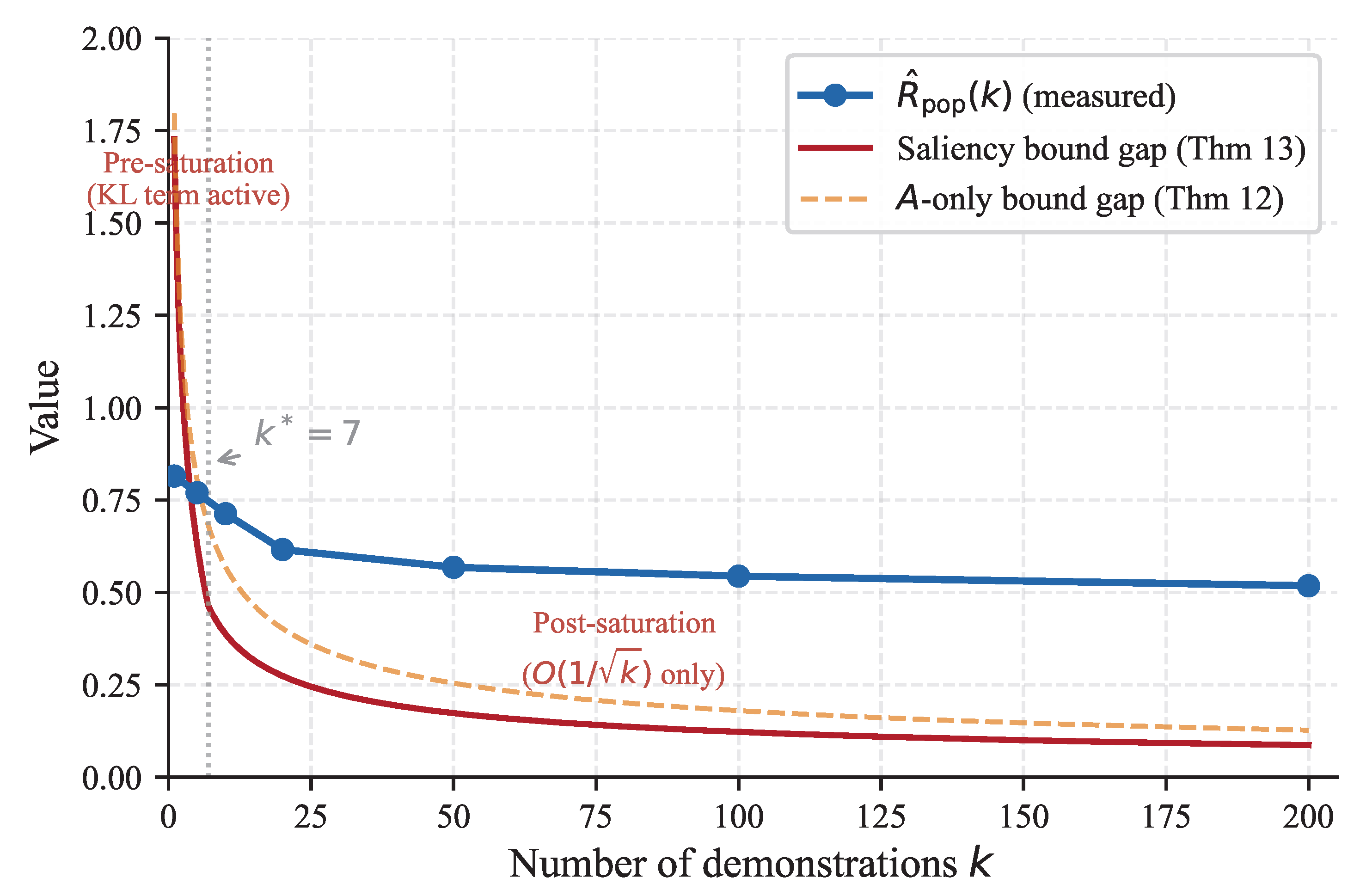
Figure 2.
Experiment 3: Saturation phase transition (Config C, , , ). (a) The KL complexity term decreases linearly to zero at (shaded region). (b) The bound gap drops rapidly in the pre-saturation regime (red) due to KL reduction, then transitions to the slower -only rate post-saturation (blue). The dashed line shows the pure confidence term .
Figure 2.
Experiment 3: Saturation phase transition (Config C, , , ). (a) The KL complexity term decreases linearly to zero at (shaded region). (b) The bound gap drops rapidly in the pre-saturation regime (red) due to KL reduction, then transitions to the slower -only rate post-saturation (blue). The dashed line shows the pure confidence term .
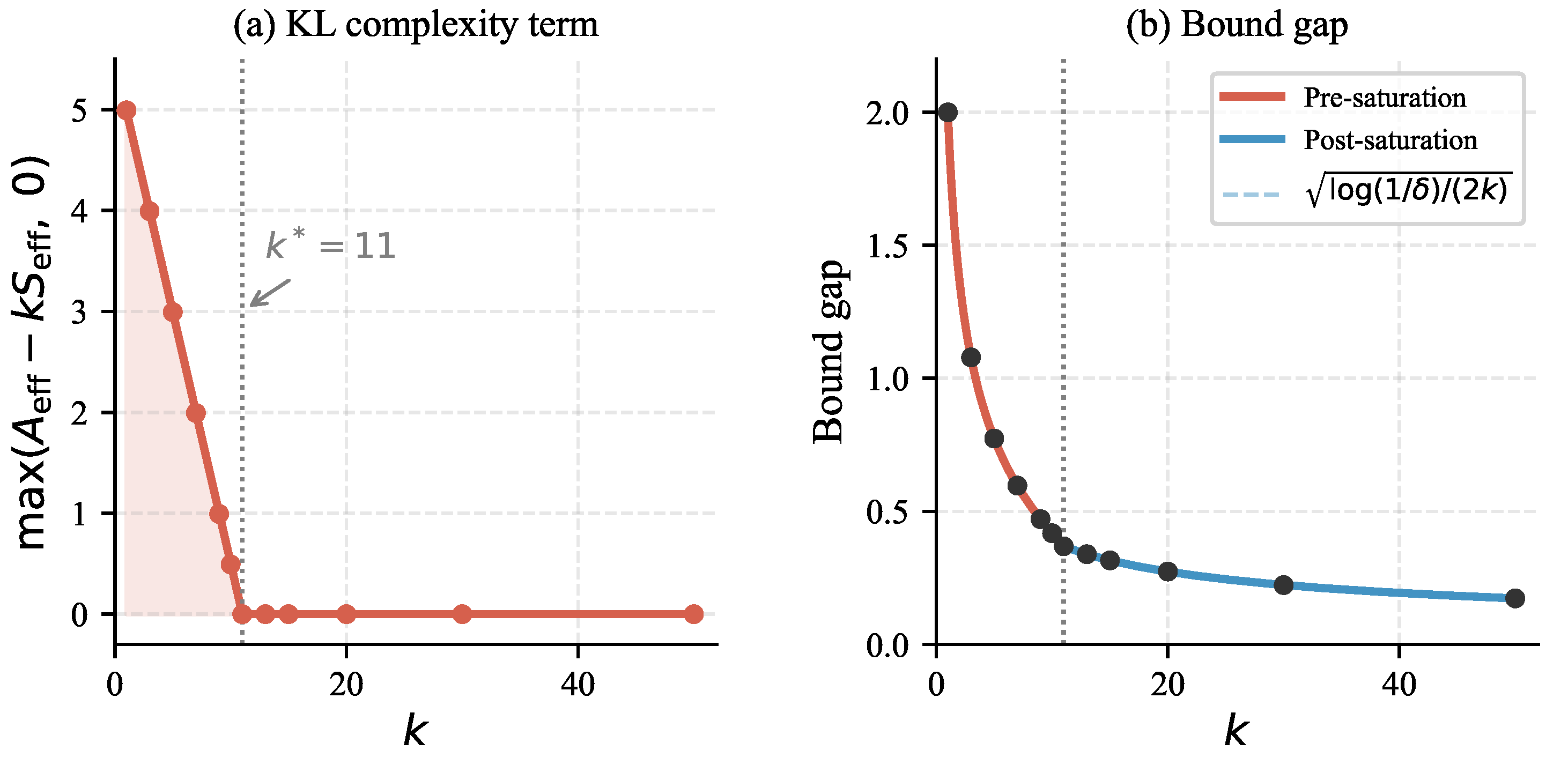
Figure 3.
Experiment 4: McAllester vs. Catoni bound comparison (Config B, , , ). The McAllester bound (blue, ) is tighter for small k; the Catoni bound (red, ) becomes tighter after the crossover at . At , the Catoni bound () is approximately half the McAllester bound ().
Figure 3.
Experiment 4: McAllester vs. Catoni bound comparison (Config B, , , ). The McAllester bound (blue, ) is tighter for small k; the Catoni bound (red, ) becomes tighter after the crossover at . At , the Catoni bound () is approximately half the McAllester bound ().
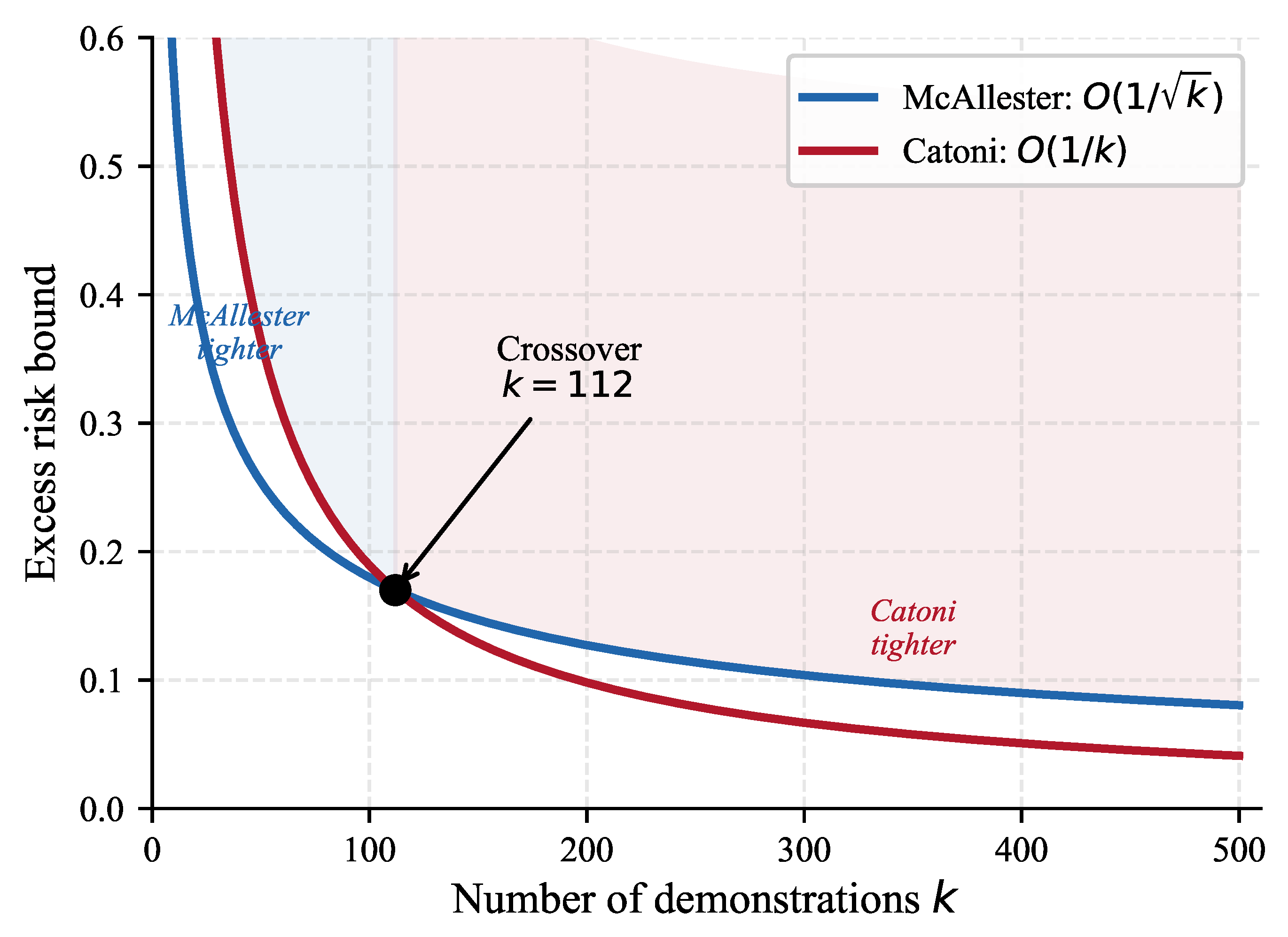
Figure 4.
Experiment 6: Measured KL divergence vs. linear Assumption A1 (SST-2, GPT-2, ). The measured KL (blue squares, with band) is approximately constant (– nats) across k, in stark contrast to the linear decrease to zero predicted by Assumption A1 (red dashed line). The core PAC-Bayes bound remains valid since for all k.
Figure 4.
Experiment 6: Measured KL divergence vs. linear Assumption A1 (SST-2, GPT-2, ). The measured KL (blue squares, with band) is approximately constant (– nats) across k, in stark contrast to the linear decrease to zero predicted by Assumption A1 (red dashed line). The core PAC-Bayes bound remains valid since for all k.
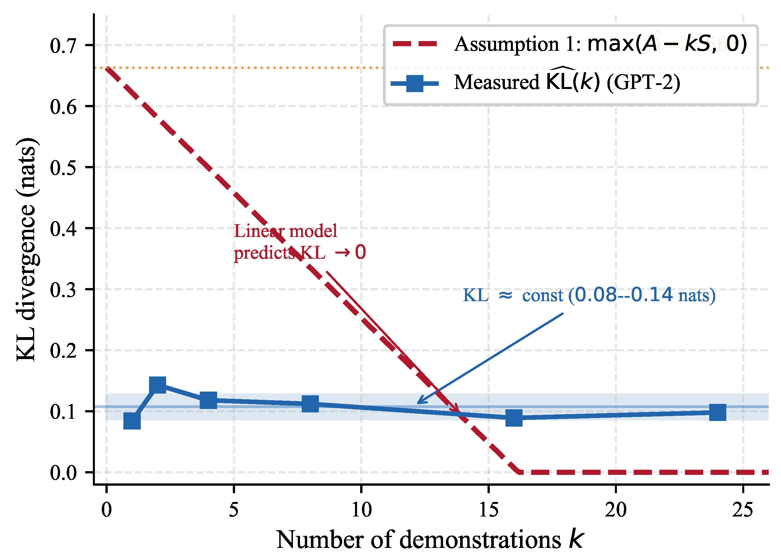
Table 1.
Comparison with existing ICL theoretical analyses. “Inf-time” indicates whether the bound applies to inference-time generalization of a frozen model (vs. pretraining analysis). “Computable” indicates whether the bound parameters are computable from the model.
Table 1.
Comparison with existing ICL theoretical analyses. “Inf-time” indicates whether the bound applies to inference-time generalization of a frozen model (vs. pretraining analysis). “Computable” indicates whether the bound parameters are computable from the model.
| Inf-time | Computable | Sample compl. | Architecture | Lower bound | Fast rate | Var-aware | |
|---|---|---|---|---|---|---|---|
| Bayesian inf. [2] | |||||||
| Gradient desc. [3] | ✓ | ||||||
| Alg. selection [5] | |||||||
| Info-theoretic [7] | ✓ | ||||||
| BMA + pretrain [8] | ✓† | ||||||
| Asymptotics [9] | ✓ | ✓ | ✓ | ||||
| This work | ✓ | ✓ | ✓ | ✓ | ✓ | ✓ | ✓ |
Table 5.
Experiment 1: Generalization bound tightness (Config C, , , ). “Gap” is the average; “Bound” is the high-probability saliency-enhanced bound from Theorem 3 (which holds with probability , not in expectation). When Gap > Bound, the average gap exceeds the high-probability bound—this is possible because the bound targets the -quantile, not the mean.
Table 5.
Experiment 1: Generalization bound tightness (Config C, , , ). “Gap” is the average; “Bound” is the high-probability saliency-enhanced bound from Theorem 3 (which holds with probability , not in expectation). When Gap > Bound, the average gap exceeds the high-probability bound—this is possible because the bound targets the -quantile, not the mean.
| k | Gap | Bound | Status | ||
|---|---|---|---|---|---|
| 1 | 0.812 | 0.029 | 0.783 | 1.999 | ✓ |
| 2 | 0.795 | 0.031 | 0.764 | 1.368 | ✓ |
| 5 | 0.773 | 0.048 | 0.725 | 0.774 | ✓ |
| 10 | 0.654 | 0.104 | 0.550 | 0.418 | † |
| 15 | 0.576 | 0.184 | 0.392 | 0.316 | † |
| 20 | 0.496 | 0.236 | 0.260 | 0.274 | ✓ |
| 30 | 0.448 | 0.287 | 0.161 | 0.223 | ✓ |
| 50 | 0.405 | 0.324 | 0.081 | 0.173 | ✓ |
†Mean gap exceeds the high-probability bound; see caption.
Table 6.
Experiment 5: PAC-Bayes bound verification with GPT-2 on SST-2 (, , , trials). “Bd(KL)” uses the measured ; “Bd(A)” uses the ambiguity upper bound. Both bound gaps decrease at the theoretical rate. All bounds hold (Rpop< Remp+ Bd).
Table 6.
Experiment 5: PAC-Bayes bound verification with GPT-2 on SST-2 (, , , trials). “Bd(KL)” uses the measured ; “Bd(A)” uses the ambiguity upper bound. Both bound gaps decrease at the theoretical rate. All bounds hold (Rpop< Remp+ Bd).
| k | Bd(KL) | Bd(A) | Valid | |||
|---|---|---|---|---|---|---|
| 1 | 0.534 | 0.800 | 0.084 | 1.241 | 1.353 | ✓ |
| 2 | 0.568 | 1.000 | 0.143 | 0.886 | 0.956 | ✓ |
| 4 | 0.525 | 0.788 | 0.118 | 0.624 | 0.676 | ✓ |
| 8 | 0.529 | 0.850 | 0.112 | 0.441 | 0.478 | ✓ |
| 16 | 0.515 | 0.731 | 0.089 | 0.311 | 0.338 | ✓ |
| 24 | 0.518 | 0.800 | 0.098 | 0.254 | 0.276 | ✓ |
Table 7.
Experiment 7: Empirically estimated ICL parameters from GPT-2 on three NLP benchmarks. and are estimated from model outputs; is the predicted saturation point. is the zero-shot risk; is the minimum risk observed over .
Table 7.
Experiment 7: Empirically estimated ICL parameters from GPT-2 on three NLP benchmarks. and are estimated from model outputs; is the predicted saturation point. is the zero-shot risk; is the minimum risk observed over .
| Task | (nats) | |||||
|---|---|---|---|---|---|---|
| SST-2 | 0.661 | 0.041 | 16 | 0.670 | 0.497 | 0.173 |
| AG News | 0.785 | 0.033 | 24 | 0.330 | 0.572 | −0.242 |
| SNLI | 0.558 | 0.023 | 24 | 0.670 | 0.645 | 0.025 |
Table 8.
Structural comparison of PAC-Bayes analyses: standard ML vs. ICL.
| Aspect | Standard ML | ICL (this work) |
|---|---|---|
| Posterior Q | Over parameters | Over predictions |
| Prior P | Design choice (e.g., ) | Pretrained zero-shot |
| measures | Parameter deviation | Prediction shift (ambiguity A) |
| Complexity driver | (model size) | A (task–model mismatch) |
| Sample complexity | , | |
| Saturation | Eventual (-dependent) | Hard, at |
| Learning mechanism | Parameter update (SGD) | Attention conditioning (frozen) |
| Fast rate condition | Low noise (Bernstein) | Low ambiguity (close prior) |
Disclaimer/Publisher’s Note: The statements, opinions and data contained in all publications are solely those of the individual author(s) and contributor(s) and not of MDPI and/or the editor(s). MDPI and/or the editor(s) disclaim responsibility for any injury to people or property resulting from any ideas, methods, instructions or products referred to in the content. |
© 2026 by the authors. Licensee MDPI, Basel, Switzerland. This article is an open access article distributed under the terms and conditions of the Creative Commons Attribution (CC BY) license (http://creativecommons.org/licenses/by/4.0/).
Copyright: This open access article is published under a Creative Commons CC BY 4.0 license, which permit the free download, distribution, and reuse, provided that the author and preprint are cited in any reuse.


