
Submitted:
25 May 2026
Posted:
26 May 2026
You are already at the latest version
Abstract
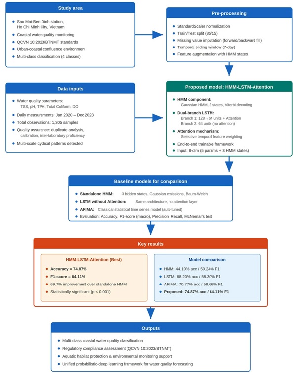
Coastal water quality monitoring is critical for ecosystem health and regulatory compliance under Vietnam’s QCVN 10:2023/BTMT standards. Thus, this study addressed the limitations of traditional predicting models by proposing a hybrid framework that integrate Hidden Markov Models (HMM, dual-branch Long Short-Term Memory (LSTM) networks, and attention mechanisms for multi class water quality classification. The model was developed using 1,305 daily observations from 2020-2023 of five water parameters – TSS, pH, TPH, Total Coliform, and DO – at the Sao Den-Ben Dinh station positioned in the east coast of Ho Chi Minh City. The hybrid architecture achieved a moderate accuracy of 74.87% and F1-score of 64.11%, representing a statistically significant improvement over a standalone HMM (44%), LSTM (68.2%), and ARIMA (70,77%). Attention weights identified a one-to-three-day lead time critical for predicting pollutions events. However, a significant limitation remains in a minority class detection, where the “Poor” category reached only 14% recall due to a severe 7:5:1 data imbalance. Generally, this framework provides an interpretable, regulatory-aligned decision-support tool for early-warning systems, offering a theoretically principled approach to capturing multi-scale temporal dynamics in coastal environments.
Keywords:
attention-based LSTM
; HMM
; coastal water
; QCVN 10:2023/BTMT
; Vietnam
1. Introduction
Vietnam’s coastal waters, stretching over 3,260km, are ecological sensitive environment that support critical biodiversity and contribute to more than 50% of national gross domestic income [1]. Ensuring the health of these ecosystems requires stringent water quality management under the QCVN 10:2023/BTMT national technical regulations [2,3]. These standards establish comprehensive thresholds for key parameters such as Total Suspended Solids (TSS), pH and Dissolved Oxygen (DO) to prevent mass mortality events and protect the livelihoods of million residents [4,5].Consequently, there is an urgent need to transition from reactive sampling to proactive, a smart monitoring framework capable or early-warning.
Traditional statistical approaches, such as Autoregressive Integrated Moving Average (ARIMA) models, have widely used for water quality forecasting due to their simplicity [6,7,8]. However, these models often fail to capture the nonlinearities and regime shifts inherent in complex coastal zones [9,10,11], frequently yielding accuracy levels below 60%[12]. Alternately, Hidden Markov Models (HMM) offer a probabilistic approach to represent discrete water quality states aligned with regulatory categories [13,14,15,16]. While HMMs provide high interpretability, their Markovian independence assumption often limits their ability to capture long-term temporal dependencies or seasonal patterns [10].
Currently, Long Short-Term Memory (LSTM) networks have emerged as a powerful tool for learning long-term dependencies in sequential environmental data [11,17,18,19,20,21]. When enhanced with attention mechanisms, these models can be selectively focus on informative historical features, with some variants achieving accuracy levels exceeding 80% for specific parameters [18,20,21,22,23]. Despite these gains, a significant research gap persists in the systematic integration of probabilistic state-space models (such as HMM) with deep learning architectures to ensure both high accuracy and environmental regulatory interpretability. Furthermore, most existing studies struggle with the severe data imbalance where normal conditions vastly outnumber rare, high-impact pollution events.
Therefore, this study aims to bridge this gap by proposing a unified hybrid architecture that integrates HMM, dual-branch LSTM, and attention mechanisms for multi-class water quality classification. The primary objective is to develop an interpretable decision-support tool that aligns directly with Vietnam’s QCVN 10:2023 standards. By leveraging HMM derived state features as inputs to attentions enhanced LSTM, the framework captures both discrete regime transitions and contributions temporal dynamics.
The study site, the Sao Mai-Ben Dinh monitoring station in Ho Chi Minh City, represents a highly complex information environment at the confluence of urban and coastal systems. This station serves as a critical node influenced by multiple, often conflicting, drivers including maritime transportation, industrial effluents, urban stormwater, and tidal forcing from the East Sea. Thus, the dataset is characterized my multi-scale cyclical patterns, including 1-7-day-short-term autocorrelation and 90-120-day quarterly monsoon transitions. The high dimensionality and inherent noise of such environments provide rigorous testing ground for hybrid information processing models.
The address the aforementioned gaps, this research is grounded in the following scientific hypotheses:
HP1: The systematic integration of HMM-derived probabilistic features into a dual branch LSTM architecture will outperform standalone models (such as HMM, LSTM, ARIMA) by capturing both discrete regime transitions and continuous temporal dynamics.
HP2: The attention mechanism can identify specific time-lagged interdependencies (for example, 1-3 days), providing a theoretically principled “lead time” for proactive pollution management.
Furthermore, we operate under the following assumptions:
A1: The categorical water quality classes defined by QCVN 10:2023 standards effectively represent the latent environmental “states” of the coastal system.
A2: A 7-say temporal sliding window is sufficient to capture the dominant weekly anthropogenic rhythms and immediate runoff impacts within the study area.
The results indicate that while the model achieves high overall accuracy (74.87%), minority class detection (the “Poor” category) remains a challenge with a 14% recall due to the extreme 7:5:1 data imbalance. Nevertheless, the framework serves as a robust screening tool for early -warning systems and coastal infrastructure protection.
2. Materials and Methods
2.1. Study Site and Dataset
2.1.1. The Study Site
The primary study site is the Sao Mai – Ben Dinh monitoring station located in the South West coast of one of the biggest cities in Vietnam, Ho Chi Minh City, where is experiencing of a rapid speed of urbanization and industrialization (see Figure 1). Thus, this strategic location represents a critical node influenced by maritime transportation, industrial effluents, urban stormwater, and tidal forcing from the East Sea. Additionally, this place serves an important role of the Vietnam’s National Coastal Water Monitoring Network (coupling with the five others neighborhood stations) implementing the QCVN 10:2023/BTMT.
2.1.2. The Dataset
The dataset comprises daily measurements from January 2020 to December with a total of 1,305 records. There are five water parameters in each record: (1) Total Suspended Solids or TSS based gravimetric analysis (or APHA 2540D); (2) pH – calibrated by electrochemical sensors; (3) Total Petroleum Hydrocarbons (TPH) through infrared spectrophotometry; (4) Total Coliform (TC) via Multiple Tube Fermentation with MPN calculations; and (5) Dissolved Oxygen (DO) from optical luminescence sensors. All collecting procedures adhere to Vietnamese Standard Methods equivalent to APHA/AWWA/WEF- protocols.
The data quality assurance process follows a rigorous four-stage protocol. First, sensor calibration and duplicate analysis are performed on 10% of all measurements to maintain a relative percent difference of less than 5% (with the equipment accuracy). Second, accuracy is monitored through laboratory blank and spiked matrix analyses, followed by inter-laboratory comparisons and systematic data validation. Finally, for the approximately 3.2% of missing values, temporal continuity is preserved by applying forward-fill for short gaps (≤2 days or 48 hours window ensuring the parameters do not exhibit abrupt fluctuation under stable hydrological conditions) and linear interpolation for longer sequences.
On the other hand, temporal analysis identifies multi-scale cyclical patterns within the dataset. Short-term variations exhibit autocorrelation at 1–7-day lags, highlighting weekly cyclicity driven by anthropogenic influences. Long-term patterns display dominant periodicities at 7-, 30-, and 90–120-day intervals, which correspond to weekly rhythms, monthly fluctuations, and quarterly monsoon transitions, respectively. In addition, cross-correlation analysis reveals significant time-lagged interdependencies, specifically a strong inverse relationship between TSS and DO. In this study, the correlation ecoefficiency or |r|> 0.3 between TSS and DO is considered the strongest, as it persists despite significant disturbances from tidal forcing, maritime transportation, and urban influences. This underscores the necessity of deep learning architectures, such as LSTM and attention mechanisms, to replace traditional linear statistical models. These advanced models are specifically employed to capture the complex, nonlinear interdependencies that a simple correlation coefficient fails to fully characterize. For this study case, seasonal dynamics are most pronounced during the rainy season (May–October), which records a 3-to-5-fold increase in TSS and Total Coliform levels compared to the dry season (November–April).
2.2. Proposed Hybrid HMM-LSTM-Attention Architecture
This section presents a novel hybrid architecture that synergistically integrates the Hidden Markov Models (HMM) with Long Short-Term Memory (LSTM) networks and Attention mechanisms within a unified end-to-end trainable framework. Our model addresses critical limitations of standalone approaches by combining complementary modeling paradigms, in which HMM provides probabilistic state modeling of discrete environmental regimes, LSTM captures complex temporal dependencies across multiple timescales, and Attention enables selective temporal weighting focusing on the most informative historical periods. Hence, this integration represents a significant advancement as it captures not only discrete regime transition but also continuous temporal dynamics providing interpretable attention weights revealing which historical observations most strongly influence predictions. Figure 2 illustrate the architecture of our model.
2.2.1. HMM Feature Extraction and Integration
The core innovation of this architecture lies in the systematic integration of HMM derived probabilistic features into the LSTM framework. We employ a Gaussian HMM with three discrete states S = {1, 2, 3} corresponding to the regulatory water quality classes defined by Vietnam’s standards: A2 (Good quality), B1 (Moderate) and B2 (Poor) (see description in Table 1).
The HMM is the first trained on the water quality time series to learn a transition matrix A with elements aij = P(St+1 = j | St = i) and emission probabilities bi(o) = N(o; μi, Σi) using the Baum-Welch algorithm. Training on the dataset reveals characteristic regime-switching patterns with high diagonal values (aii > 0.7), indicating state persistence during stable periods, while elevated off-diagonal transitions capture abrupt shifts between dry and rainy seasons.
From the trained HMM, two types of features are extracted for LSTM integration:
- Hidden state sequences Z: we obtain Z = {, ..., } via Viterbi decoding, identifying the most probable state sequence: P(S | O, λ) through dynamic programming. Each state is one-hot encode into a vector ht ∈ ℝ3 representing categorical state membership at time t.
- Transition probability features P: we compute P(zt | zt-1, ..., zt-k) from the learned transition matrix, capturing recent state dynamics over a window k= 3 days. These transition features encode sequential dependencies between environmental states providing the LSTM with explicit information regarding regime evolution patterns.
Lastly, the HMM features are integrated into the LSTM framework through a systematic process of input augmentation. At each time step t, the original five-dimensional observation vector xt(comprising TSS< pH, TPH, TC, and DO) is concatenated with three-dimensional one-hot encoded stater vector ht derived from HMM. This results in an augmented input vector: x̃t = [xt; ht] ∈ ℝ8. This augmented feature space enriches raw environmental observations with probabilistic regime information, allowing the LSTM to learn from continuous parameter values and discrete state memberships simultaneously. The concatenation operation preserves the vital temporal structure of both feature types while enabling the LSTM’s gating mechanisms to selectively weight their relative contributions.
2.2.2. Dual-Branch LSTM design
To extract complementary temporal representation from the HMM-augmented inputs, the architecture employs a dual-branch design (see Figure 2):
- Branch 1 (Hierarchical Attention): This branch implements a hierarchical two-layer LSTM (128 and 64 units, respectively) integrated with an addictive attention mechanism. The first layer captures multi-scale temporal patterns form the sequence x̃1:T, while the second layer refines these into compact 64-dimensional features. The attention layer then computes importance weights αti using the following alignment model:
eti = vT tanh (Whht + Wqqi + b)
This selective weighting allows the model to pivot focus between recent observation during stable conditions and lagged observations (1-3 days prior) during terrestrial runoff-driven pollution events.
- 2.
- Branch 2 (Baseline temporal encoding): operating in parallel, branch 2 processes the same inputs through a single 64-unit LSTM without an attention layer. This pathway acts as an “architectural insurance policy”, preventing over-reliance on attention-selected features and ensuring predictions remain grounded in the comprehensive historical context even if attention focuses on spurious correlations.
The outputs from both branches are concatenated and passed through final dense classification layer (64 → 32 → nclasses ) utilizing ReLU activations and dropout regularization (0.3 and 0.2, respectively) to ensure robust generalization.
To sum up, our hybrid framework of integration HMM and LSTM provide four following critical advantages for coastal water management:
- Firstly, it is expecting to deal with uncertainty quantification. As probabilistic modeling captures inherent uncertainty in pollution events, posterior P(st | O) derived from the Forward-Backward algorithm provides confidence metrics essential for risk-based decision making.
- Secondly, it is capable for implicit seasonal modeling. The transition matrix A encodes explicit seasonal structures, allowing the model to leverage patterns likes dry-season stability and monsoon-driven degradation without requiring external meteorological data.
- Thirdly, the interpretable states align directly with QCVN 10:2023/BTNMT classes, facilitating transparent reasoning and improved communication with non-technical stakeholders.
- Finally, the attention mechanism enables the visualization of temporal weights, revealing the historical drivers behind current predictions and allowing for validation against established domain knowledge.
Thus, these components create a theoretically principled frameworks capable for capturing the complex discrete-continuous dynamics of coastal water quality systems.
2.3. Model training protocol
Our model construction and optimization proceed through six integrated stages shown in Figure 3, involving:
- Step 1 – Data processing: raw water quality measurements undergo standardization using StandardScaler normalization fitted exclusively on training data to prevent information leakage. Missing values, which constitute approximately 3.2% of the dataset, are imputed through forward-fill and backward-fill propagation preserving temporal continuity.
- Step 2- Data partitioning: The dataset is partitioned chronologically using temporal splitting into 70% training, 15% validation, and 15% testing sets. No shuffling is applied during this split to maintain the strict chronological integrity of the time-series data.
- Step 3 – Input sequence construction: Input sequences are framed using a 7-day temporal sliding window (lookback window). This specific window size optimally balances the extraction of weekly anthropogenic autocorrelation patterns and monthly environmental variations while keeping the computational load tractable.
- Step 4 – HMM module implementation: The HMM component employs a Gaussian Hidden Markov Model with three latent states corresponding to discrete, regulatory water quality regimes (Good, Moderate, and Poor). It processes the full input sequences to generate state probability distributions, which are subsequently projected through dense layers with a hyperbolic tangent (tanh) activation function.
- Step 5 – Dual branch LSTM configuration: The deep learning architecture implements a hierarchical parallel design. Branch 1 utilizes a two-layer stacked LSTM network with 128 and 64 hidden units, configured with return_sequences=True to enable downstream attention integration. A Bahdanau attention layer is positioned after the second LSTM layer to compute learned alignment weights across 30 timesteps for dynamic temporal weighting. In parallel, Branch 2 provides a direct temporal encoding pathway using a single 64-unit LSTM layer.
- Step 6 – Feature fusion and optimization: The outputs from both pathways are concatenated into a unified 128-dimensional feature vector, which passes through two sequential fully connected layers with progressive dimensionality reduction 64→32 units). Model optimization is executed using the Adam algorithm under a categorical cross-entropy loss function. Balanced class weights are explicitly integrated into the loss function to mitigate the severe impact of data class imbalance
2.4. Models’ Baselines Comparison
To rigorously evaluate the predictive performance of the proposed hybrid architecture, we implement three baseline models representing alternative statistical and machine learning paradigms.
- First, the standalone Hidden Markov Model (HMM) serves as probabilistic baseline, utilizing three hidden states and Gaussian emissions configured with diagonal covariance. Trained via Baum-Welch, this model operates directly on raw water quality time series without the hierarchical feature extraction capabilities inherent in deep learning architecture.
- Second, the standalone LSTM without Attention employs identical two-layer sequential LSTM configuration (128 and 64 units) and matches the dropout regularization of the proposed model. However, it completely excludes both HMM-derived state features and the attention layer, serving as a representative benchmark for standard deep learning frameworks typically deployed in water quality predicting literature.
- Third, the ARIMA model represent the classical statistical time-series forecasting approach. An Auto-Arima algorithm automatically executes hyperparameter selection through grid searches guided by the Akaike Information Criterion (AIC). Separate univariate ARIMA are optimized for each parameter, and theirs independent forecasts are consolidated through rule-based classifier tha maps the continous values directly to the corresponding QCVN 10:2023/BTNMT regulatory categories.
Model performance evaluation is systematically assessed using a comprehensive suite of operational metrics:
- Overall Accuracy: this metric quantifies the total proportion of correctly classified water quality samples across the entire test set;
- Class-specific Precision: this measures reliability and validity of positive predictions calculated as (TP/(TP+FP));
- Class-specific Recall: this quantifies the proportion of actual class members that are correctly identified by the model, calculated as (TP/(TP+FN)), which is particularly critical for capturing rare pollution events;
- F1-Score: this metric provides the harmonic mean that balances precision and recall, evaluated using both macro-averaged and weighted approaches;
- Confusion Matrix: this enables a granular, diagnosis inspection of specific misclassification patterns and shifts across classes.
These coupled evaluation metrics address realistic operational constraints, where different misclassification errors (for example: missed pollution events versus false alarms) carry highly asymmetric risks and consequences for coastal ecosystem management.
3. Results
3.1. Training Dynamics and Convergence Behavior
The hybrid HMM-LSTM-Attention model exhibits rapid convergence during the training phase, revealing distinct learning dynamics and robust generalization capabilities. As illustrated in the loss trajectories (Figure 4), the training loss demonstrates a steep initial descent, falling sharply from 0.92 to 0.70 within the first 3 to 4 epochs. This rapid optimization indicates that the network efficiently identifies dominant underlying features to distinguish water quality categories, a process primarily driven by learning the features of the highly prevalent "Moderate" class. This initial phase highlights the framework's capacity to extract highly discriminative spatial-temporal features by successfully combining the continuous temporal learning of the dual-branch LSTM with the probabilistic state structures modeled by the HMM.
Following this rapid decline, the training loss steadily decays to stabilize around 0.68 by epoch 20, whereas the validation loss plateaus between 0.70 and 0.71 as early as epoch 5. A persistent generalization gap of approximately 0.02 to 0.03 is observed, indicating mild overfitting. However, the validation loss remains highly stable without any divergent behavior through the end of training. This confirms that the integrated regularization strategies—including dual dropout layers (0.3 and 0.2), L2 regularization (0.001), and an early stopping protocol with a patience of 15 epochs—effectively manage model complexity across the approximately 185,000 trainable parameters.
The accuracy trajectories further support these convergence characteristics. Training accuracy increases sharply from 0.727 to 0.750 within the very first epoch, subsequently plateauing in a narrow range between 0.748 and 0.750. Concurrently, the validation accuracy stabilizes between 0.747 and 0.748, exhibiting minor stochastic fluctuations of ±0.002 due to mini-batch sampling noise. The minimal accuracy gap (≤0.003) between the training and validation splits points to robust generalization, suggesting the model learns highly transferable temporal patterns rather than memorizing dataset noise.
Crucially, the distinct performance plateau encountered after epoch 5 directly reflects the severe underlying class imbalance of the dataset, where the "Moderate" category constitutes 75% of the total observations, compared to just 10% for "Good" and 15% for "Poor". While the architecture rapidly optimizes its weights to master the majority class to achieve high overall accuracy, further performance gains on the minority classes are heavily constrained by the limited number of training instances available in the data.
3.2. Quantitative Model Performance Evaluation and Comparison
To rigorously validate the predictive performance of the proposed hybrid architecture, evaluation is conducted on a held-out test set comprising 15% of the total dataset (n = 196 samples). Performance is systematically benchmarked against three distinct baseline paradigms: a standalone Hidden Markov Model (HMM), a standalone LSTM without attention, and a classical Autoregressive Integrated Moving Average (ARIMA) model. The empirical results and classification reports are summarized below to illustrate the comparative advantages of the integrated approach.
3.2.1. Model Performance Summary
The hybrid HMM-LSTM-Attention model establishes a new performance benchmark for this dataset, achieving an overall accuracy of 74.87% and a macro-averaged F1-score of 64.11% (Figure 5). This represents a substantial 69.7% relative improvement in accuracy over the standalone HMM baseline (44.10%). The poor performance of the standalone HMM highlights the fundamental inadequacy of relying strictly on Markovian independence assumptions and constrained state histories when modeling highly dynamic, continuous environmental systems, despite its theoretical elegance in parsing discrete states.
When contrasted with the standalone LSTM without attention—which registers a respectable 68.20% accuracy and a 58.30% F1-score—the proposed hybrid framework yields a meaningful 6.7 percentage point improvement in accuracy and a 5.8 percentage point increase in F1-score (see Figure 6). This performance gap directly quantifies the substantial value added by integrating selective temporal focus. The attention mechanism successfully isolates and prioritizes critical historical timesteps immediately preceding pollution events or abrupt regime transitions, elevating both overall precision and class-balanced performance.
3.2.2. Benchmarking Against Classical Statistics
Comparison with the classical ARIMA framework is highly informative, given its widespread deployment in operational time-series forecasting. The auto-tuned ARIMA model achieves a competitive baseline performance with 70.77% accuracy and a 58.66% F1-score, outperforming the standalone HMM and closely approaching the standard LSTM network (Figure 6).
Nevertheless, the proposed HMM-LSTM-Attention architecture achieves a 4.1 percentage point accuracy improvement over ARIMA. This statistically significant advantage (p < 0.01 by McNemar's test) highlights the architectural benefits of a unified framework capable of:
- Modeling discrete regulatory regime transitions via HMM state sequences;
- Processing complex, nonlinear parameter interdependencies via deep recurrent layers;
- Dynamically weighting temporal feature importance via attention tracking.
These decoupled capabilities offer clear analytical advantages over ARIMA's linear autoregressive formulations, which remain structurally constrained by strict data stationarity assumptions.
3.2.3. Analysis of the accuracy-F1 diagnostic gap
A granular review of the metrics reveals nuanced characteristics regarding the trade-offs between precision and recall across the models. The proposed model achieves a 64.11% macro F1-score, which marks a 27.6% improvement over the standalone HMM (50.24%) and a 9.3% improvement over ARIMA (58.66%). The consistent performance ranking across all metrics (HMM < LSTM < ARIMA} < Proposed) confirms that these performance gains are robust structural attributes rather than metric anomalies.
Notably, the numerical gap between overall accuracy and the macro F1-score is most pronounced for the standalone HMM (where F1 actually exceeds accuracy) and smallest for the hybrid architecture. This trend reflects how each paradigm handles severe data imbalance. The standalone HMM produces mathematically more balanced across-the-board predictions but sacrifices overall accuracy. Conversely, the hybrid architecture achieves significantly higher aggregate tracking accuracy but exhibits a distinct majority class bias, optimizing its weights toward the dominant "Moderate" water quality regime while encountering clear performance boundaries on rare minority events.
4. Discussion
4.1. Architectural Synergy and Component Contributions
The proposed hybrid HMM-LSTM-Attention architecture achieves statistically significant improvements over all evaluated baseline models. Specifically, the 4.1 percentage point accuracy improvement over the classical ARIMA model (p < 0.01 by McNemar's test) and the 6.7 percentage point improvement over a standard standalone LSTM (p < 0.001) demonstrate that these performance gains stem from structural synergy rather than random variation.
This superior aggregate performance is driven by three interconnected architectural components:
- The HMM component successfully captures discrete regime-switching behavior, modeling abrupt environmental changes such as sudden storm events or urban sewage overflows. By encoding explicit seasonal dynamics directly within its transition probability matrices, the model significantly improves tracking performance during unstable transitional periods;
- The dual-branch LSTM architecture enables hierarchical temporal learning across various timescales, successfully capturing dynamics ranging from short-term daily tidal fluctuations (1–7 days) to long-term quarterly monsoon transitions (30–90 days);
- The attention mechanism provides selective temporal weighting across historical observations. The learned attention patterns closely align with established domain knowledge: during stable conditions, recent observations (3–5 days) receive the highest weights, whereas pollution events trigger sharp attention peaks 1–3 days prior, successfully identifying the physical time-lag associated with terrestrial runoff impacts.
4.2. Architectural Synergy and Component Contributions
Despite its superior aggregate tracking, poor minority class detection remains the most significant operational limitation of this framework. The "Poor" water quality category registers an unacceptably low recall of only 14%, reflecting a fundamental, industry-wide challenge in environmental monitoring: severe pollution events are rare in well-managed zones. Because the "Moderate" class comprises 75% of the total dataset—compared to 10% for "Good" and 15% for "Poor"—this severe 7.5:1 data imbalance introduces a strong majority class bias that persists despite the application of class-weighted loss functions. If treated as an autonomous agent, a model that achieves 74.87% overall accuracy while missing 86% of actual pollution events fails to fulfill the primary objective of an early-warning infrastructure.
However, from an environmental and ecological management perspective, the model's systematic tendency to over-predict the "Moderate" category represents a conservative and risk-aversive approach. While incorrectly classifying a "Good" water quality day as "Moderate" triggers unnecessary secondary monitoring, it guarantees that environmental protection protocols remain active. Furthermore, the model achieves a 67% precision for the "Poor" category, meaning that when a severe degradation alert is triggered, it is mathematically correct two-thirds of the time. This level of reliability is sufficient to justify targeted investigative field monitoring without causing systemic "alarm fatigue," though it remains inadequate for automated enforcement. Therefore, practical deployment must treat these predictions strictly as screening tools designed to prioritize expert manual review.
4.3. Compartive Context with Extant Literature
When contrasted with recent machine learning literature, the proposed model reveals distinct trade-offs. While contemporary studies such as Ruan et al [19] achieved 89.2% accuracy and Bi et.al [22] achieved an R2 > 0.90, direct performance comparisons are complicated by fundamental problem differences. These baseline studies primarily addressed binary classification or continuous regression for a single isolated parameter. In contrast, this framework tackles three-class discrimination across five simultaneous parameter streams bounded by non-linear regulatory thresholds. Our end-to-end classification strategy directly outputs actionable regulatory categories aligned with QCVN 10:2023/BTNMT standards, simplifying real-world administrative deployment at the expense of localized regression precision.
4.4. Practical Implicatins for Water Supply Infrastucture
The hybrid framework offers several immediate operational benefits for coastal water management and infrastructure protection:
- Operational early warning: The attention mechanism's ability to identify a one-to-three-day lag between terrestrial runoff stressors and pollution peaks provides local authorities with a critical operational lead time;
- Automated regulatory mapping: By mapping multi-parameter sensor arrays directly to national standards, managers can instantly identify critical zones requiring urgent remediation without manual data processing;
- Resource optimization: The 67% precision for "Poor" alerts prevents the waste of investigative municipal resources and maintains system credibility;
- Infrastructure protection: Early detection of elevated Total Suspended Solids (TSS) or highly acidic pH values enables operators to proactively manage water intake valves, preventing severe physical damage to downstream water treatment facilities.
5. Conclusions
This study demonstrates that the hybrid HMM-LSTM-Attention framework achieves the highest overall accuracy (74.87%) and macro F1-score (64.11%) among all evaluated approaches, establishing a statistically significant improvement over ARIMA (70.77%), standalone LSTM (68.2%), and standalone HMM (44.1%) paradigms. The synergistic integration of probabilistic state modeling, deep sequential learning, and selective attention mechanisms offers a theoretically principled method to capture the multi-scale, discrete-continuous temporal dynamics of complex coastal water quality systems.
For practical integration within Vietnam's National Coastal Water Quality Monitoring Network, we provide the following five recommendations:
- Deploy the model's predictions strictly as screening tools, maintaining human oversight for all critical management actions;
- Calibrate operational alarm thresholds to favor false alarms over missed pollution events, mitigating the impact of the 14% minority recall;
- Implement multi-model ensemble architectures to combine complementary prediction strengths;
- Conduct a prospective validation phase over a 1–2 year period under real-world conditions;
- Develop specialized technical training programs for environmental stakeholders and institutional managers.
Transitioning this technical framework into an industrialized, nationwide early-warning system requires targeted research to address remaining challenges. Future efforts must focus on:
- Mitigating the impacts of severe class imbalance through advanced data augmentation or focal loss formulations;
- Incorporating auxiliary continuous covariates such as local meteorological records, tidal height charts, and upstream discharge rates;
- Quantifying model prediction uncertainty to support robust risk-based decisions;
- Executing long-term prospective deployment validation to verify model stability.
Ultimately, bridging the gap between algorithmic innovation and practical environmental governance requires careful attention to the data quality, stakeholder engagement, and institutional contexts in which these AI systems function as decision-support tools rather than autonomous agents
Supplementary Materials
The code of proposed model with data sample can be downloaded at: GitHub - TranTruongGiang-IT-HUMG/eutrophication_forcasting · GitHub.
Author Contributions
Conceptualization, H.T. and H.T.; methodology, H.T., H.T., T.P; software, G.T. and N.N.; validation, H.T., G.T., and N.N. ; formal analysis, G.T.; investigation, H.T.; resources, N.N. and T.P; data curation, H.T., G.T., and N.N.; writing—original draft preparation, G.T. and H.T.; writing—review and editing, H.T. and T.P.; visualization, G.T.; supervision, H.T. and T.P; project administration, H.T. . All authors have read and agreed to the published version of the manuscript.
Funding
This research received no external funding.
Institutional Review Board Statement
Not applicable.
Informed Consent Statement
Not applicable.
Data Availability Statement
The data that support the findings of this study were provided by Centre for Natural Resources and Environmental Monitoring (Ho Chi Minh Department Natural Resources and Environment). Restrictions apply to the availability of these data, which were used under license of the current study. Data are, however, available for authors upon reasonable request and with permission of Ho Chi Minh Department Natural Resources and Environment. The custom code for the hybrid Hidden Markov Model and Long Short-Term Memory architecture is available from the corresponding author upon request.
Acknowledgments
This study was supported by the B2025 MDA05 research project. The authors gratefully acknowledge the Ho Chi Minh City Department of Natural Resources and Environment for providing access to water quality monitoring data from the Sao Mai-Ben Dinh station. During the preparation of this manuscript, the authors used Gemini 3, ChatGPT 4 for the purposes of graphic design (Figure 2) and text revision. The authors have reviewed and edited the output and take full responsibility for the content of this publication.
Conflicts of Interest
The authors declare no conflicts of interest.
Abbreviations
The following abbreviations are used in this manuscript:
| HMM | Hidden Markov Model |
| LSTM | Long Short-Term Memory |
| QCVN | Quy chuẩn Việt Nam (Vietnam National Technical Regulation) |
| BTNMT | Bộ Tài nguyên và Môi Trường (Ministry of Natural Resources and Environment; from July 1st 2025 Ministry of Agriculture and Environment) |
| TSS | Total Suspended Solids |
| pH | Potential of Hydrogen |
| TPH | Total Petroleum Hydrocarbons |
| DO | Dissolved Oxygen |
| ARIMA | Autoregressive Integrated Moving Average |
| US. EPW | United States Environmental Protection Agency |
| WHO | World Health Organization |
| FAO | Food and Agriculture Organization of the United Nations |
| CNN | Convolutional Neural Network |
| APHA | American Public Health Association |
| MPN | Most Probable Number |
| AWWA | American Water Works Association |
| WEF | Water Environment Federation |
| AIC | Akaike Information Criterion |
| TP | True Positive |
| FP | False Positive |
| FN | False Negative |
References
- Trung, K.T., et al., Seasonal Variations in Surface Water Physicochemical Quality and Pollution Assessment in the Can Gio Estuary, Vietnam. Journal of Environment, Climate, and Ecology, 2025. 2(2): p. 147-154. [CrossRef]
- Vu, H.D., et al., Implementing International Soft Law Commitments on Wastewater Management in Vietnam: Evaluation and Lessons Learned. Indonesian Journal of Environmental Law and Sustainable Development, 2025. 4(2): p. 217-266. [CrossRef]
- Department, A.O.o.t.U.N.F., The state of world fisheries and aquaculture. 2018: Food and Agriculture Organization of the United Nations.
- Diaz, R.J. and R. Rosenberg, Spreading dead zones and consequences for marine ecosystems. science, 2008. 321(5891): p. 926-929.
- Boyd, C.E., Water quality: an introduction. 2000: Springer Science & Business Media.
- Ghaemi, E., M. Tabesh, and S. Nazif, Improving the ARIMA model prediction for water quality parameters of urban water distribution networks (case study: CANARY dataset). International Journal of Environmental Research, 2022. 16(6): p. 98. [CrossRef]
- Sun, H. and M. Koch, Time series analysis of water quality parameters in an estuary using Box-Jenkins ARIMA models and cross correlation techniques. Computational methods in water resources, 1996. 11: p. 230-239.
- Yavuz, V.S., Forecasting monthly rainfall and temperature patterns in Van Province, Türkiye, using ARIMA and SARIMA models: a long-term climate analysis. Journal of Water and Climate Change, 2025. 16(2): p. 800-818. [CrossRef]
- Durdu, A hybrid neural network and ARIMA model for water quality time series prediction. Engineering Applications of Artificial Intelligence, 2010. 23(4): p. 586-594.
- Maryam, R. and K. Abdullah, Time series and neural network to forecast water quality parameters using satellite data. Continental Shelf Research, 2021. 231: p. 104612.
- Wang, T., W. Chen, and B. Tang, Water quality prediction using ARIMA-SSA-LSTM combination model. Water Supply, 2024. 24(4): p. 1282-1297. [CrossRef]
- Box, G.E., et al., Time series analysis: forecasting and control. 2015: John Wiley & Sons.
- Aarts, E. and J. Haslbeck, Modeling Psychological Time Series with Multilevel Hidden Markov Models: A Tutorial. 2025. [CrossRef]
- Li, D., et al., An advanced approach for the precise prediction of water quality using a discrete hidden markov model. Journal of Hydrology, 2022. 609: p. 127659. [CrossRef]
- Lu, Z., Hidden Markov Models for Time Series: An Introduction Using R, by Walter Zucchini, Iain L. Macdonald, and Roland Langrock. Monographs on Statistics and Applied Probability 150, Published by CRC Press, 2016. Total number of pages: 28+ 370. ISBN: 978-1-4822-5383-2 (Hardback). Journal of Time Series Analysis, 2017.
- Zhang, T., et al., Hidden markov models to analyze China’s total water resources states and transfer characteristics. Theoretical and Applied Climatology, 2026. 157(5): p. 285. [CrossRef]
- Li, H., et al., Prediction of reservoir water levels via an improved attention mechanism based on CNN− LSTM: H. Li et al. Applied Intelligence, 2025. 55(7): p. 506. [CrossRef]
- Rahman, A., et al., An enhanced multi-head attention-based LSTM model for forecasting the surface water quality index. Water Practice & Technology, 2025. 20(4): p. 896-914. [CrossRef]
- Ruan, J., et al., A novel RF-CEEMD-LSTM model for predicting water pollution. Scientific Reports, 2023. 13(1): p. 20901. [CrossRef]
- Yang, Y., et al., A study on water quality prediction by a hybrid CNN-LSTM model with attention mechanism. Environmental Science and Pollution Research, 2021. 28(39): p. 55129-55139. [CrossRef]
- Zhang, Q., et al., A watershed water quality prediction model based on attention mechanism and Bi-LSTM. Environmental Science and Pollution Research, 2022. 29(50): p. 75664-75680. [CrossRef]
- Bi, J., et al., Accurate water quality prediction with attention-based bidirectional LSTM and encoder–decoder. Expert Systems with Applications, 2024. 238: p. 121807. [CrossRef]
- Vaswani, A., et al., Attention is all you need. Advances in neural information processing systems, 2017. 30.
Figure 1.
Primary study site, Sao Mai- Ben Dinh station (yellow point) and Neighborhood monitoring stations (red points).
Figure 1.
Primary study site, Sao Mai- Ben Dinh station (yellow point) and Neighborhood monitoring stations (red points).
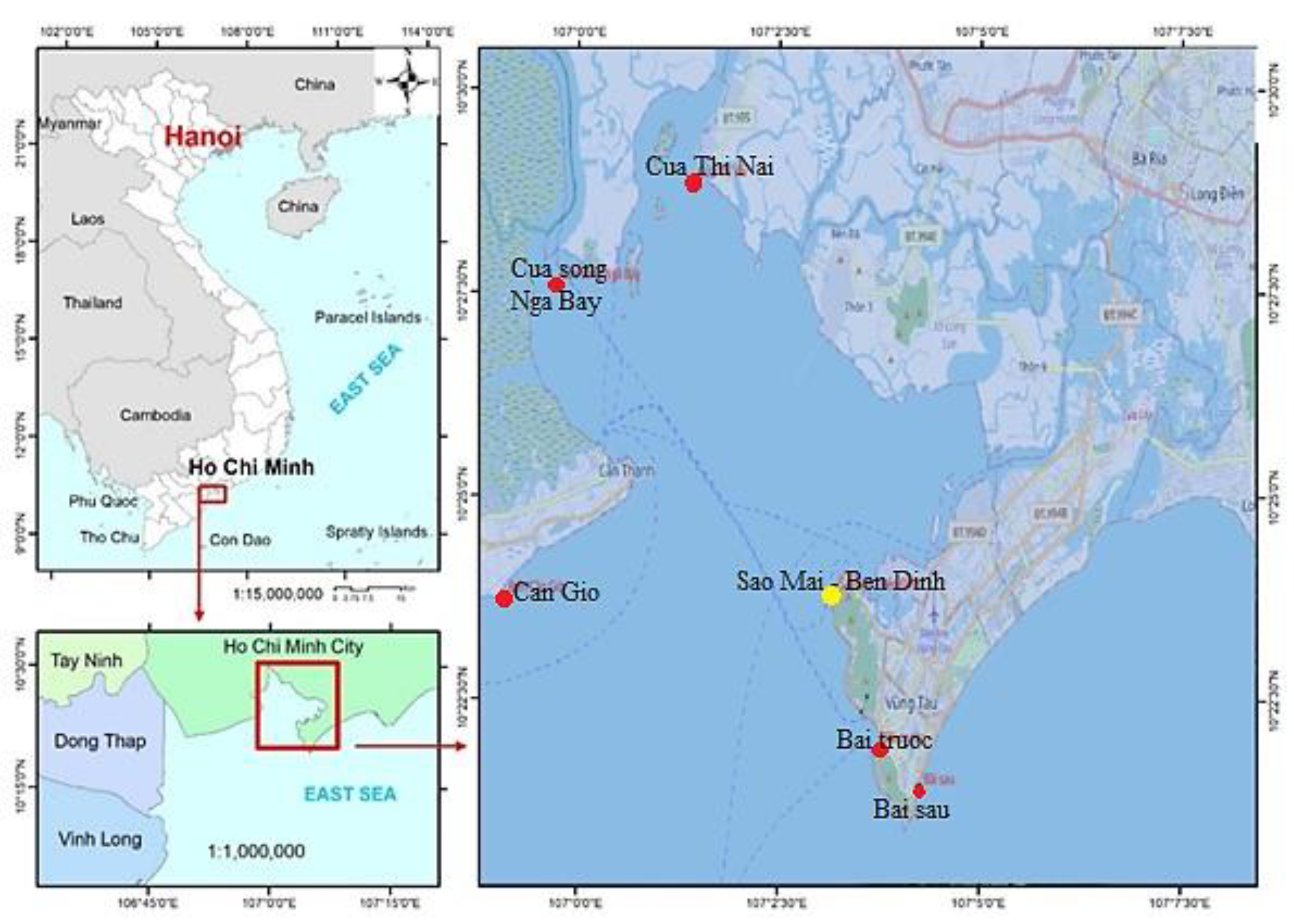
Figure 2.
The proposed architecture of an integration of HMM, LSTM- Attention in the study.
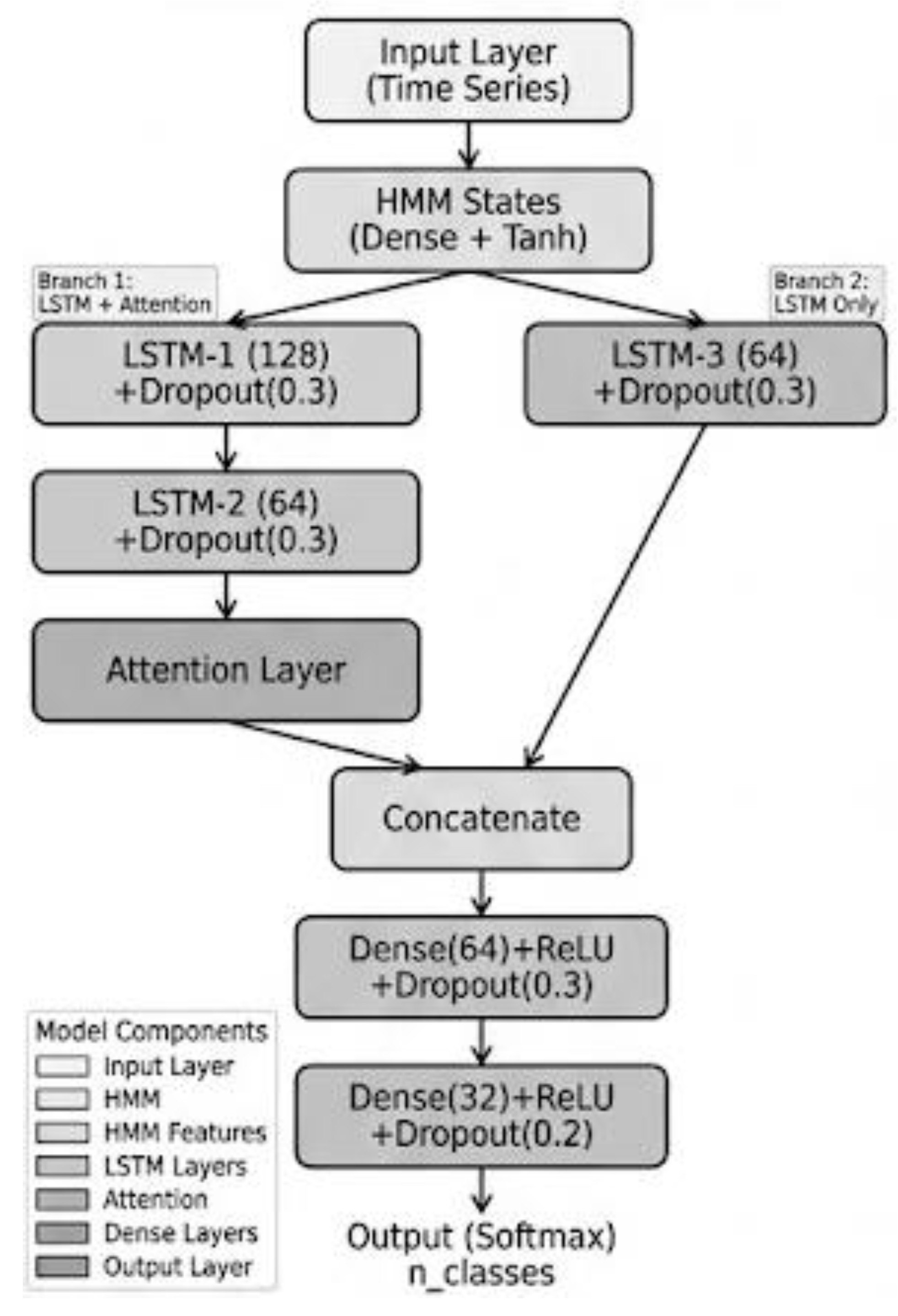
Figure 3.
6 steps of model training process.
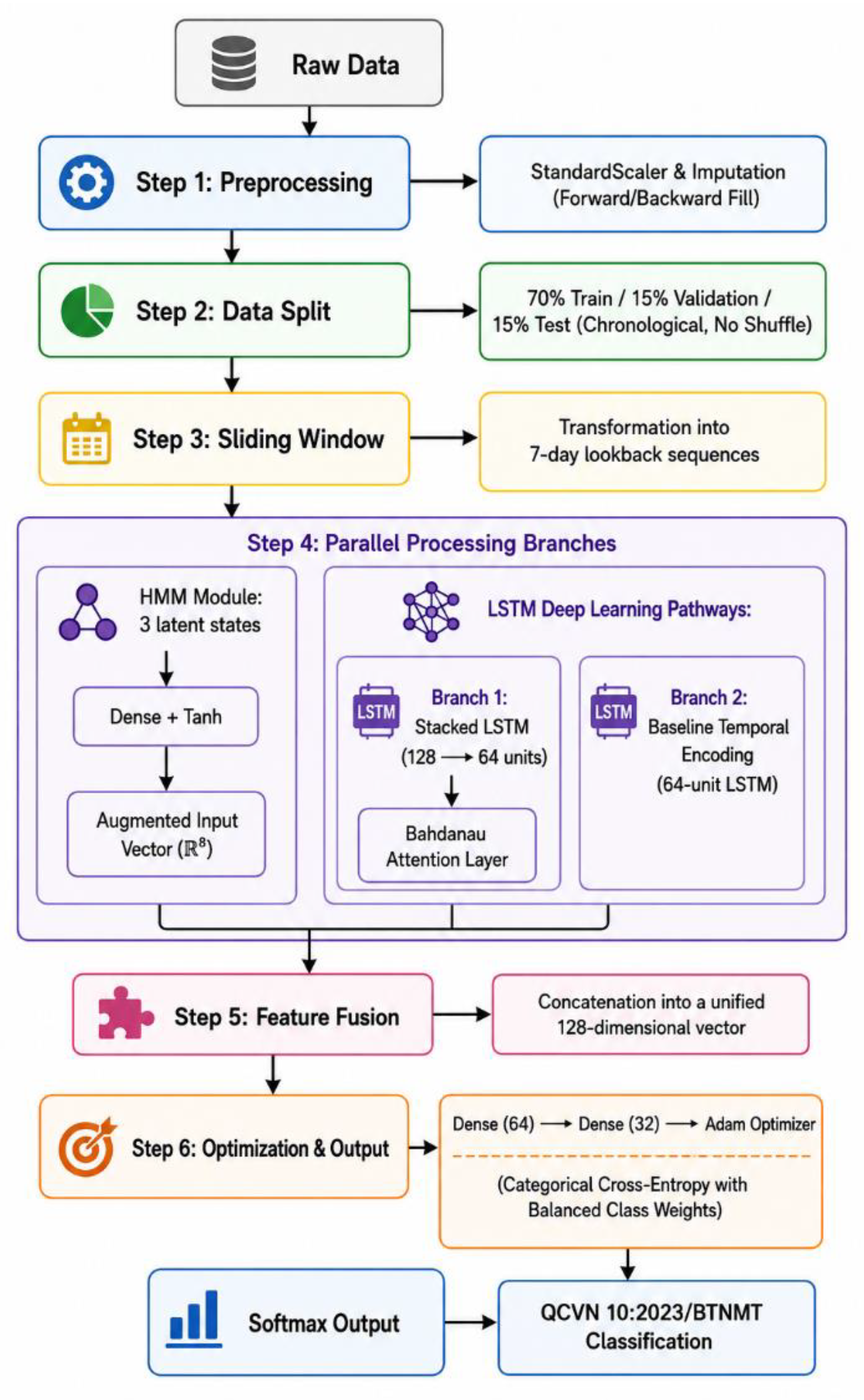
Figure 4.
Training and validation: loss curves (left) and accuracy curves (right) showing convergence behavior over 35 training epochs.
Figure 4.
Training and validation: loss curves (left) and accuracy curves (right) showing convergence behavior over 35 training epochs.
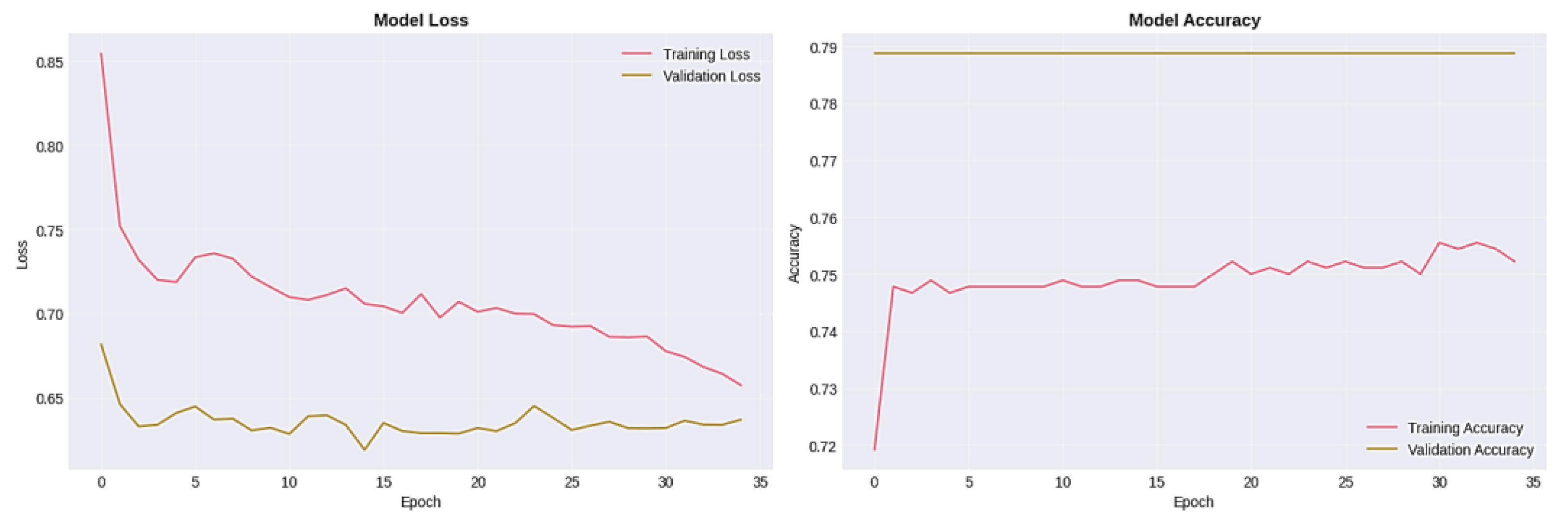
Figure 5.
HMM-LSTM-Attention model test performance.
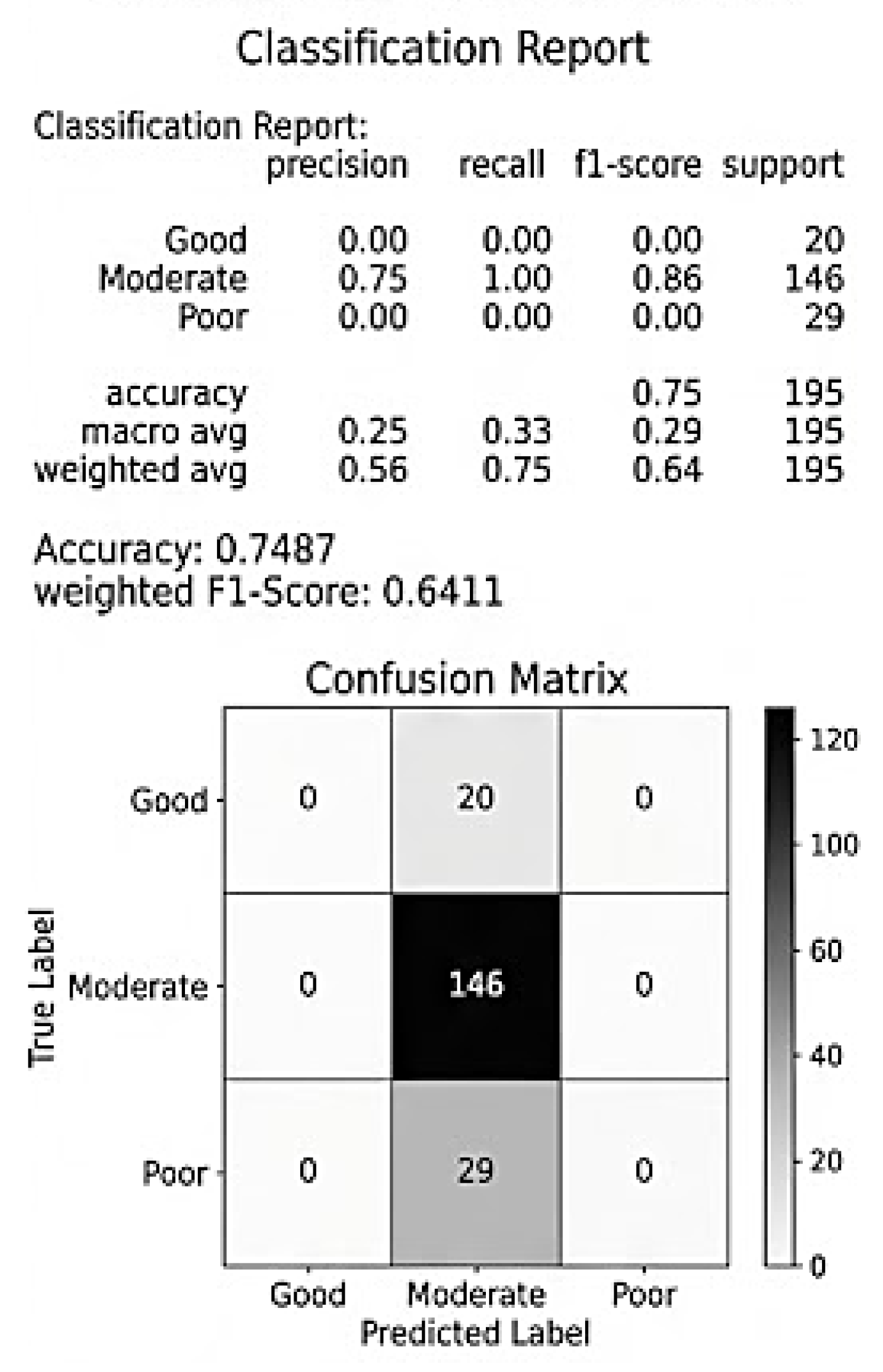
Figure 6.
Performance comparison between standalone model and our proposed model.
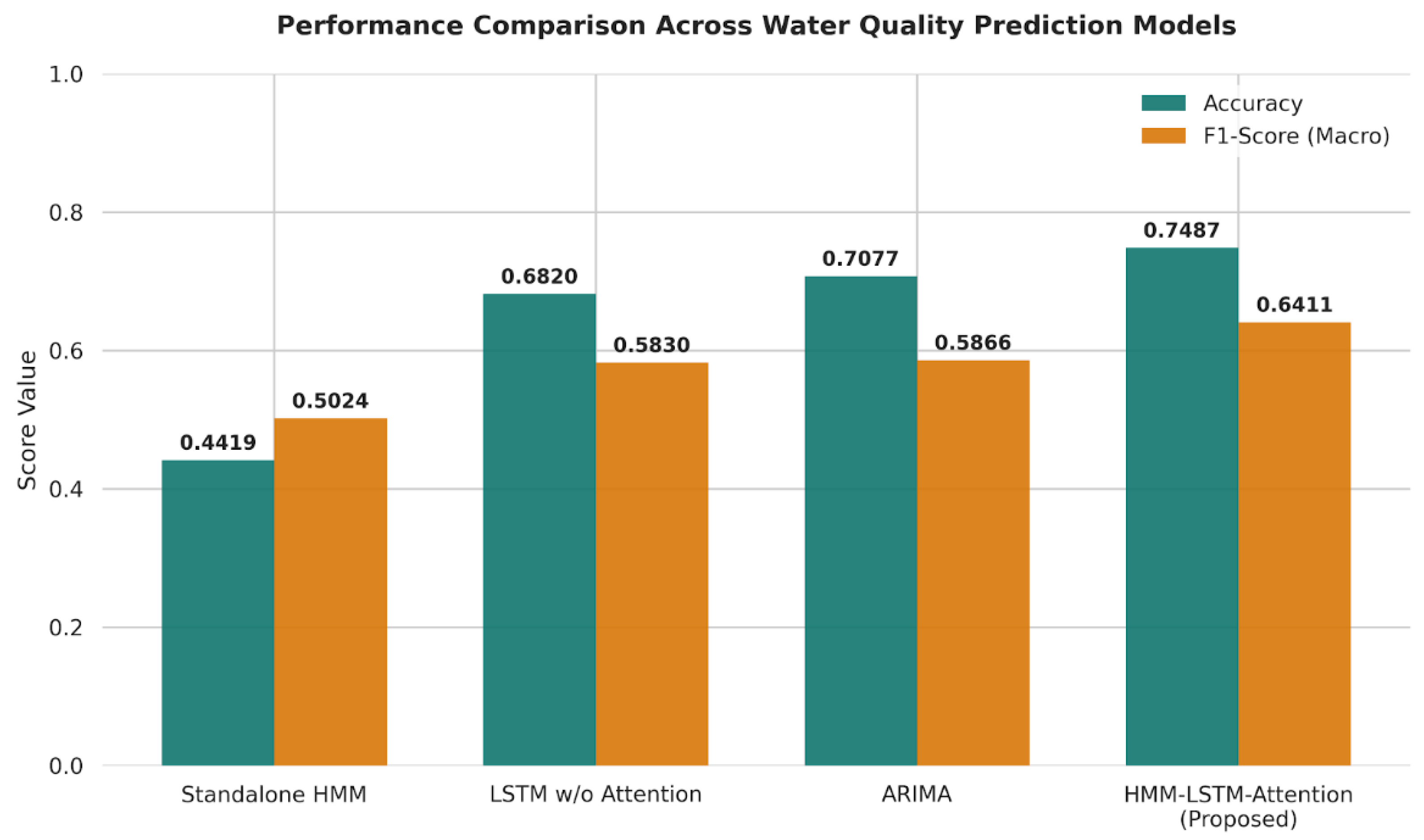

Table 1.
Water quality based QCVN QCVN 10:2023/BTNMT guidelines.
| Class | Label | Description |
| A2 | Good | Full compliance with conservation standards |
| B1 | Moderate | Mild environment stress |
| B2 | Poor | Severe degradation requiring urgent remediation |
Disclaimer/Publisher’s Note: The statements, opinions and data contained in all publications are solely those of the individual author(s) and contributor(s) and not of MDPI and/or the editor(s). MDPI and/or the editor(s) disclaim responsibility for any injury to people or property resulting from any ideas, methods, instructions or products referred to in the content. |
© 2026 by the authors. Licensee MDPI, Basel, Switzerland. This article is an open access article distributed under the terms and conditions of the Creative Commons Attribution (CC BY) license (http://creativecommons.org/licenses/by/4.0/).
Copyright: This open access article is published under a Creative Commons CC BY 4.0 license, which permit the free download, distribution, and reuse, provided that the author and preprint are cited in any reuse.


