
Submitted:
19 May 2026
Posted:
26 May 2026
You are already at the latest version
Abstract
Modeling a user's evolving goals, values, and affect over time is central to perspective-aware AI, yet progress is bottlenecked by the lack of longitudinal data with ground-truth labels for latent identity state. We introduce PAiNT (Perspective-Aware AI Identity and Narrative Toolkit), a generative framework that simulates long-horizon persona trajectories and emits corresponding multimodal artifacts with ontology-aligned labels of the latent identity state that produced them. PAiNT decouples identity dynamics from artifact generation via a typed Persona Matrix and Situation Graph, coordinated through a multi-agent loop with validation-gated transitions and bounded-window history conditioning. Across four personality archetypes, four backbone LLMs, and three architectural ablations, evaluated with a nine-metric suite calibrated on published longitudinal data, we find that (i) persona initialization produces a durable identity signal that persists above stochastic event noise; (ii) multi-agent orchestration and history conditioning govern distinct quality dimensions, with removal of either causing different failure modes; and (iii) a coherence frontier constrains the trade-off between temporal resolution and horizon, with substantial penalties at daily granularity. We release PAiNT and PAi-Bench, a human-validated benchmark of 1,200 labeled multimodal artifacts, at: https://anonymous.4open.science/r/paint-0411/.
Keywords:
perspective-aware AI
; synthetic data generation
; longitudinal persona simulation
; multiagent LLM systems
1. Introduction
Humanity is entering a new phase of human-machine symbiosis where AI systems are no longer just tools, but also persistent partners embedded in the fabric of daily life. Yet, today’s AI systems are fundamentally perspective-blind: they lack a persistent, evolving representation of a specific user’s goals, values, affect, and constraints. This limitation matters most in longitudinal settings, where users rely on AI not only for isolated queries but also for extended tasks such as navigating career change, managing health decisions, coordinating complex workflows, or interacting within extended reality (XR) environments [14]. In such settings, effective support requires more than stylistic personalization or retrieval of recent context; it requires modeling how a user’s internal state changes over time.
A central obstacle to this goal is a severe data bottleneck. Learning to model evolving user perspective would require longitudinal digital footprints—for example, emails, chats, calendars, and decision traces—spanning months or years. In practice, such data is difficult to use for research because it is privacy-sensitive, fragmented across proprietary silos, and largely unlabeled with respect to internal state [32,33]. We may observe what a user wrote or did, but not directly why they acted, what they felt, or which constraints shaped the decision. As a result, progress on perspective-aware AI is limited not only by modeling challenges but also by the absence of auditable, structurally supervised longitudinal datasets.
Perspective-Aware AI (PAi) offers a useful conceptual frame for addressing this gap. In PAi, a user’s evolving perspective is represented explicitly through a structured object—a Chronicle—that can encode goals, values, affect, and social context over time. Under this view, the problem is not only to generate personalized outputs, but to model and maintain an explicit representation of the perspective that gives rise to them [8,34]. However, data-driven methods for building and evaluating such systems remain constrained by the lack of suitable training and benchmarking resources.
To address this problem, we introduce PAiNT (Perspective-Aware AI Identity and Narrative Toolkit), a generative framework for simulating long-horizon persona trajectories and producing paired outputs: multimodal digital artifacts together with explicit, ontology-aligned labels of the latent identity state that produced them. PAiNT decouples identity dynamics from artifact generation through three core structures: a Persona Matrix that tracks evolving identity attributes, a Persona Path that records event-driven state transitions, and a Situation Graph that encodes the entity’s perspective in each local situation. Because identity state is explicit rather than implicit in an LLM context window, it can be inspected, ablated, and quantitatively evaluated, making the resulting data structurally supervised and suitable for controlled experimentation.
Figure 1.
The structured Persona Matrix (1), the ontology-aligned Situation Graph label (2), and the generated multimodal artifacts (3), evolving longitudinally across T timesteps (4). The Situation Graph serves as a supervised signal for downstream inference tasks, while multimodal artifacts are conditioned cross-modally on the unified situation state.
Figure 1.
The structured Persona Matrix (1), the ontology-aligned Situation Graph label (2), and the generated multimodal artifacts (3), evolving longitudinally across T timesteps (4). The Situation Graph serves as a supervised signal for downstream inference tasks, while multimodal artifacts are conditioned cross-modally on the unified situation state.
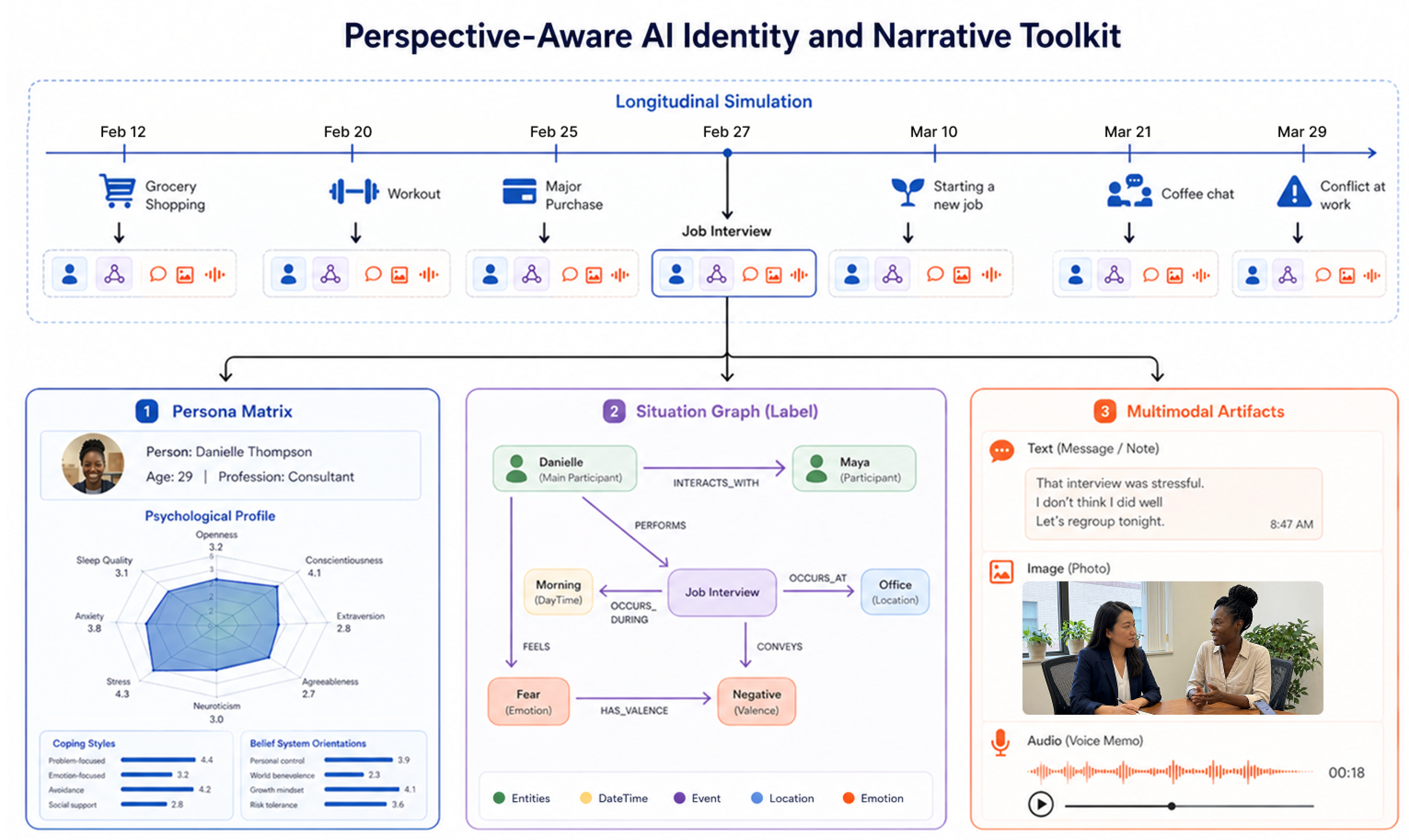
Our contributions are fourfold:
- 1.
- We introduce PAiNT, a state-conditioned generative framework that decouples latent identity dynamics from observable artifacts. This design exposes identity state as explicit supervision, enabling controlled ablation, drift analysis, and future downstream learning on synthetic longitudinal data.
- 2.
- We provide a systematic evaluation of PAiNT across archetypes, temporal configurations, backbones, and architectural ablations. This evaluation identifies which components govern which quality dimensions and characterizes a coherence frontier between temporal resolution and simulation horizon.
- 3.
- We introduce a reusable metric suite for longitudinal identity simulation, including temporal drift diagnostics calibrated from published longitudinal data, a three-phase narrative coherence pipeline, and cross-modal graph-alignment metrics.
- 4.
- We release PAi-Bench, a benchmark of longitudinal, multimodal, perspective-labeled digital footprints generated with PAiNT and curated with human oversight, to support future research on perspective-aware AI and longitudinal perspective inference.
Together, PAiNT and PAi-Bench provide a structured foundation for generating, evaluating, and benchmarking synthetic longitudinal perspective data without relying on real user histories.
2. Related Work
PAiNT lies at the intersection of persona simulation, longitudinal user modeling, commonsense reasoning, and perspective-aware AI. The most important distinction from prior work is that PAiNT makes evolving identity state explicit, structured, and inspectable, rather than leaving it implicit in prompts, memories, or latent model behavior. This explicit-state design enables supervision, controlled ablation, and drift analysis over long horizons.
2.1. Persona Simulation and Generative Agents
Early work on personalized generation showed that explicit user profiles can improve dialogue consistency. Li et al. [18] introduced speaker embeddings for persona-consistent neural conversation models, and Zhang et al. [3] proposed Persona-Chat, where dialogue is conditioned on textual persona descriptions. Mazaré et al. [24] later scaled persona-based modeling using large collections of Reddit user profiles.
Large language models enabled more realistic and longer-horizon simulations. Thoppilan et al. [23] demonstrated sustained conversational behavior in LaMDA, while Park et al. [2] introduced Generative Agents, where agents evolve through memory streams and produce believable social behavior over time. However, in these systems, the state governing behavior is largely implicit. This limits direct inspection, controlled manipulation of identity variables, and quantitative analysis of how internal perspective changes over time. PAiNT differs by externalizing this state into a structured Persona Matrix and aligned Situation Graphs, making the simulated identity trajectory directly available for supervision and analysis.
Related work has also explored synthetic persona-grounded data generation. Jandaghi et al. [4] proposed a generator–critic framework for producing high-quality persona-grounded dialogues, and Chan et al. [5] introduced PersonaHub to generate large-scale synthetic personas. These efforts focus primarily on static persona specification or dialogue generation. To maintain persona coherence over extended horizons without exceeding context limits, recent architectures have also explored identity-driven retrieval-augmented generation [17]. By contrast, PAiNT targets longitudinal digital footprints and pairs generated artifacts with explicit internal-state labels, enabling structurally supervised learning rather than only artifact-level generation.
2.2. Longitudinal Modeling and Commonsense Reasoning
Long-term personalization requires representations that remain useful over extended interaction histories. Ning et al. [6] proposed User-LLM, which compresses historical user information into embeddings for personalization and retrieval. Such approaches are useful for scalability, but the resulting representations are not directly interpretable and are therefore less suitable when explicit perspective variables, state tracing, or drift analysis are required.
Our work is also related to commonsense reasoning about latent mental state. Rashkin et al. [10] introduced Event2Mind, which infers intents and emotional reactions from events, and Sap et al. [11] developed ATOMIC, a large commonsense knowledge graph encoding causal and social if–then relations. These resources model generic regularities about human behavior. In contrast, PAiNT models the perspective of a particular individual in a particular situation. Its Situation Graphs ground latent goals, affect, and interpretations in temporally situated identity trajectories rather than in population-level commonsense templates alone.
PAiNT is further grounded in the Perspective-Aware AI (PAi) framework of Alirezaie et al. [13,15], which introduces Chronicles as user-centered knowledge structures for representing goals, values, and affect over time. PAiNT operationalizes this idea for synthetic data generation: each Situation Graph captures a localized slice of perspective, while a sequence of such graphs forms a longitudinal trajectory consistent with the broader notion of a Chronicle. By generating these graphs together with multimodal artifacts, PAiNT produces the paired supervision needed for downstream perspective-inference tasks such as Situation Graph Prediction, which we identify as a key direction for future work.
2.3. Bias, Ethics, and Perspective-Awareness
PAiNT is motivated in part by the limitations of one-size-fits-all foundation models. Bender et al. [7] characterized such models as “stochastic parrots,” warning that they lack contextual understanding, while Bommasani et al. [20] argue that foundation models tend to homogenize users by defaulting to statistical averages. These concerns are especially relevant when systems are expected to interact with users whose goals, values, and interpretations differ systematically from population norms.
Prior work has documented such harms empirically. Sheng et al. [9] showed that neural text generation can exhibit gender and racial biases, and Lucy and Bamman [19] found stereotyped portrayals in generated narratives. Lewicki et al. [8] further argue that fairness cannot be assessed independently of context, and Weidinger et al. [25] catalog broader risks of large-scale language models, including misalignment with user needs and values.
While alignment methods such as RLHF [22] improve general helpfulness, they optimize toward a generic user preference rather than explicitly modeling user-specific perspective. Real-world multimodal datasets such as Ego4D [21] capture rich first-person experience, but they do not provide direct labels for the internal states that shape observable behavior and may be difficult to use because of privacy and governance constraints. PAiNT is intended as a complementary alternative: it generates privacy-safe, auditably labeled longitudinal data in which the internal states that produce observable behavior are exposed explicitly, enabling controlled research on perspective-aware modeling without direct access to sensitive real-world histories.
3. Problem Setting and Design Requirements
We study the problem of generating longitudinal, perspective-labeled digital footprints for a single focal entity (an individual) over a time horizon T. PAiNT is designed primarily as an open-ended persona simulator and data generator, and secondarily as a source of structured labels that can support downstream modeling of latent perspective state.
3.1. Generative Setting and Outputs
Let denote a user-provided persona scaffolding, instantiated as a structured schema of identity constraints, and let denote the generation configuration, including the random seed, temporal resolution, horizon, event taxonomy, and modality policy. A PAiNT run takes as input and generates a temporally ordered sequence of situations indexed by discrete timesteps . The simulation is initialized with an identity state derived from the input schema using a model (such as an LLM):
and an initial history summary , which may be empty or derived from . Here, T denotes the simulation horizon, and the terminal identity state.
At each timestep, the framework produces four coupled objects:
Specifically:
- is the Persona Matrix, representing the entity’s identity state at time t. It contains both relatively stable attributes (e.g., background factors and enduring traits) and dynamic attributes (e.g., goals, affect, relationships, stress, and habits) that may evolve over time.
- is the exogenous event or situation trigger at time t (e.g., “job interview,” “conflict with teammate,” “health setback,” “product launch”), sampled from a controlled taxonomy.
- is the Situation Graph, an ontology-aligned structured representation of the entity’s perspective in the current situation, including variables such as goals, affect, appraisal, social roles, constraints, and salience. Within the simulated dataset, it serves as the structured label for downstream supervised or self-supervised tasks.
- is a set of multimodal artifacts emitted at time t (e.g., messages, emails, photos, phone calls, or voice memos), treated as partial and noisy observations of the underlying state and situation.
3.1.1. State-Conditioned Dynamics
The simulated persona trajectory is modeled as a state-conditioned process. At each timestep t, the event is sampled according to an event-transition mechanism , conditioned on the previous identity state and a bounded history summary . The identity state is then updated through a transition mechanism :
The history summary is computed by a history aggregation function over bounded windows of prior identity states and events:
where k and m are user-defined history context window sizes for past Persona Matrix states and events, respectively. For early timesteps, when the full window is not yet available, these sequences are truncated to the observed prefixes. Here, denotes the ordered sequence , and is defined analogously.
Given the current state , event , and history summary , the Situation Graph is constructed by a labeling function , and the observable artifacts are generated by an artifact generator :
This factorization separates identity evolution (), perspective labeling (), and artifact generation (). Consequently, PAiNT generates longitudinal multimodal trajectories together with structured labels , while enabling controlled ablations and analysis of identity drift through the explicit state sequence .
3.2. Downstream Use Cases
PAiNT is designed to support controlled training and evaluation for perspective-aware modeling tasks. Given observations , which may be noisy, partial, and multimodal, a downstream model may be asked to:
- 1.
- infer (state estimation),
- 2.
- infer (perspective labeling),
- 3.
- predict future events or states such as or (forecasting), or
- 4.
- detect inconsistencies, anomalies, or regime shifts over time (diagnostics).
Because PAiNT provides structured latent states and perspective labels together with observable artifacts, these tasks can be evaluated directly while still allowing realistic uncertainty and partial observability through .
3.3. Design Requirements
To support controlled generation and reliable evaluation, PAiNT is designed around seven core requirements:
- R1: Factorized Control. The generator should support independent manipulation of priors, temporal resolution, and horizon length in order to enable systematic ablation studies.
- R2: Temporal Coherence. Identity dynamics should preserve stable traits while allowing bounded, event-driven evolution of dynamic attributes.
- R3: Causal Consistency. Generated trajectories should satisfy causal plausibility and narrative non-contradiction, with deterministic validation where possible.
- R4: Ontological Grounding. Structured outputs () should conform to fixed schemas so that label spaces remain stable and comparable across runs.
- R5: Cross-Modal Alignment. Generated artifacts () should remain consistent with the underlying perspective labels (), supporting downstream inference from noisy observations.
- R6: Auditability. Seeds, configurations, prompts, and generation traces should be logged to support reproducibility and inspection.
- R7: Privacy Safety. The framework should generate diverse and rich persona data without requiring sensitive real-world user histories.
Taken together, these requirements define PAiNT as a controlled and auditable framework for generating longitudinal, perspective-labeled datasets with explicit state structure, explicit temporal dynamics, and measurable validity properties. The following sections describe how the architecture and generation pipeline operationalize these requirements and how they are assessed in the evaluation protocol.
4. PAiNT Framework
PAiNT is a generative pipeline that: (i) simulates a user-defined persona’s internal and external experiences over time and (ii) produces a corresponding multimodal digital footprint grounded in the simulated persona trajectory. Its core design principle is the decoupling of latent identity dynamics—how a person changes—from the observable artifacts they emit—what a person writes, says, or photographs. This matches the formal separation between state transitions () and artifact generation () established in Section 3, and it is this property that makes PAiNT’s outputs structurally supervised: because identity state remains explicit and inspectable, it can serve as structured supervision for downstream perspective-inference tasks, be independently manipulated for ablation, and be quantitatively analyzed for drift and coherence.
PAiNT is implemented as a structured, multi-stage generative pipeline with validation-gated transitions and bounded retries. Long-horizon coherence is maintained through bounded history conditioning using recent states and events. This mechanism instantiates the design requirements introduced in Section 3, especially factorized control (R1), temporal coherence (R2), ontological grounding (R4), auditability (R6), and privacy safety (R7).
The framework comprises eight stages organized into three phases:
- 1.
- Persona Initialization (Stages 1–3), which constructs the initial persona specification, event space, and initial state.
- 2.
- Persona Trajectory Simulation (Stages 4–5), which generates the longitudinal state–event trajectory and supporting label registry.
- 3.
- Artifact Generation (Stages 6–8), which produces Situation Graphs and multimodal artifacts conditioned on the simulated trajectory.
Figure 2 summarizes the data flow. We first introduce the main data structures, then describe the three phases of the pipeline, followed by implementation details and the downstream task enabled by the generated data.
4.1. Core Data Structures
PAiNT operates over five principal data structures: the input persona scaffolding , the event taxonomy , the time-indexed Persona Matrix , the longitudinal Persona Path , and the Situation Graph associated with each timestep.
4.1.1. Persona Scaffolding ().
The Persona Scaffolding is the user-populated input schema that specifies high-level identity constraints for the initial persona state. In our implementation, it is organized into eight typed dimensions: demographic identity, professional life, personality and mindset, motivations and goals, decision-making style, social context, frustrations, and notable preferences. Each dimension is represented through a validated sub-schema with explicit field definitions. This scaffolding provides the controllable starting point of the simulation: users may fix selected identity attributes while leaving others underspecified for the generator to complete consistently.
4.1.2. Event Taxonomy ()
The Event Taxonomy is a fixed, versioned catalogue of life events used to constrain the event space. In our implementation, it contains 260 events organized into 14 categories, including educational events, career milestones, relationship dynamics, emotional stressors, daily-life situations, and technological interactions. Because is loaded from a static specification file, event selection remains reproducible and auditable across runs. Using a controlled taxonomy also limits open-ended hallucination and enables systematic ablations over event categories (R1).
4.1.3. Persona Matrix ().
The Persona Matrix is a temporally indexed, structured representation of identity state. It encodes both constant traits that must remain invariant across all timesteps (e.g., handedness, eye color, ethnicity) and dynamic attributes (e.g., stress level, coping styles, relationships, goals) that evolve in response to events. The schema comprises fourteen semantically distinct feature clusters:
- 1.
- Personality Features: Big Five (OCEAN) traits on continuous scales in ;
- 2.
- Physical Traits: embodiment features—categorical strings (hair color, ethnicity, gender, skin tone) and continuous floats (height in cm, weight in lbs). Constant.
- 3.
- Physical Health: health metrics (BMI as continuous float, fitness level on ).
- 4.
- Mental Health: stress and anxiety levels on , depression symptoms (string list).
- 5.
- Demographic Features: strings (name, profession, nationality, education, marital status) and enumerated categories (age group, income class).
- 6.
- Family & Friends: typed relationship list with closeness scores on .
- 7.
- Coping Styles: avoidance, impulsivity, emotional reactiveness, emotional regulation, escapism on .
- 8.
- Wellness & Lifestyle: work–life balance on , sleep quality (enumerated), work style (enumerated), screen time on hrs, nutrition quality on .
- 9.
- Belief System: existential, nihilist, humanist, stoic orientations and political leaning on ; religion (string).
- 10.
- Goals: short-term and long-term objectives (string lists); life driver narrative (string).
- 11.
- Fears: aversive motivations and vulnerabilities (string list).
- 12.
- Habits: communication style (enumerated), quirks (string list), irritants (string list).
- 13.
- Interests: hobbies, general interests, social affiliations (all string lists).
- 14.
- Constant Features: immutable categorical strings (handedness, eye color). Constant.
Every field is typed and range-constrained via a rigid schema that is enforced programmatically at every state transition, satisfying ontological grounding (R4). Validator agents are instructed to enforce that constant clusters remain unchanged and that numeric attributes stay within their declared bounds.
4.1.4. Persona Path ().
Personality traits are not static; longitudinal studies confirm that major life events drive measurable trait-level change, with the magnitude varying by individual rigidity and life stage [35]. The Persona Path is the longitudinal backbone of the simulation. At each timestep t, it records the event and the resulting updated state . Informally, each transition captures an event, the persona’s reaction to that event, and the state update induced by it. The Persona Path therefore constitutes the canonical latent trajectory from which all downstream labels and artifacts are derived.
4.1.5. Situation Graph ().
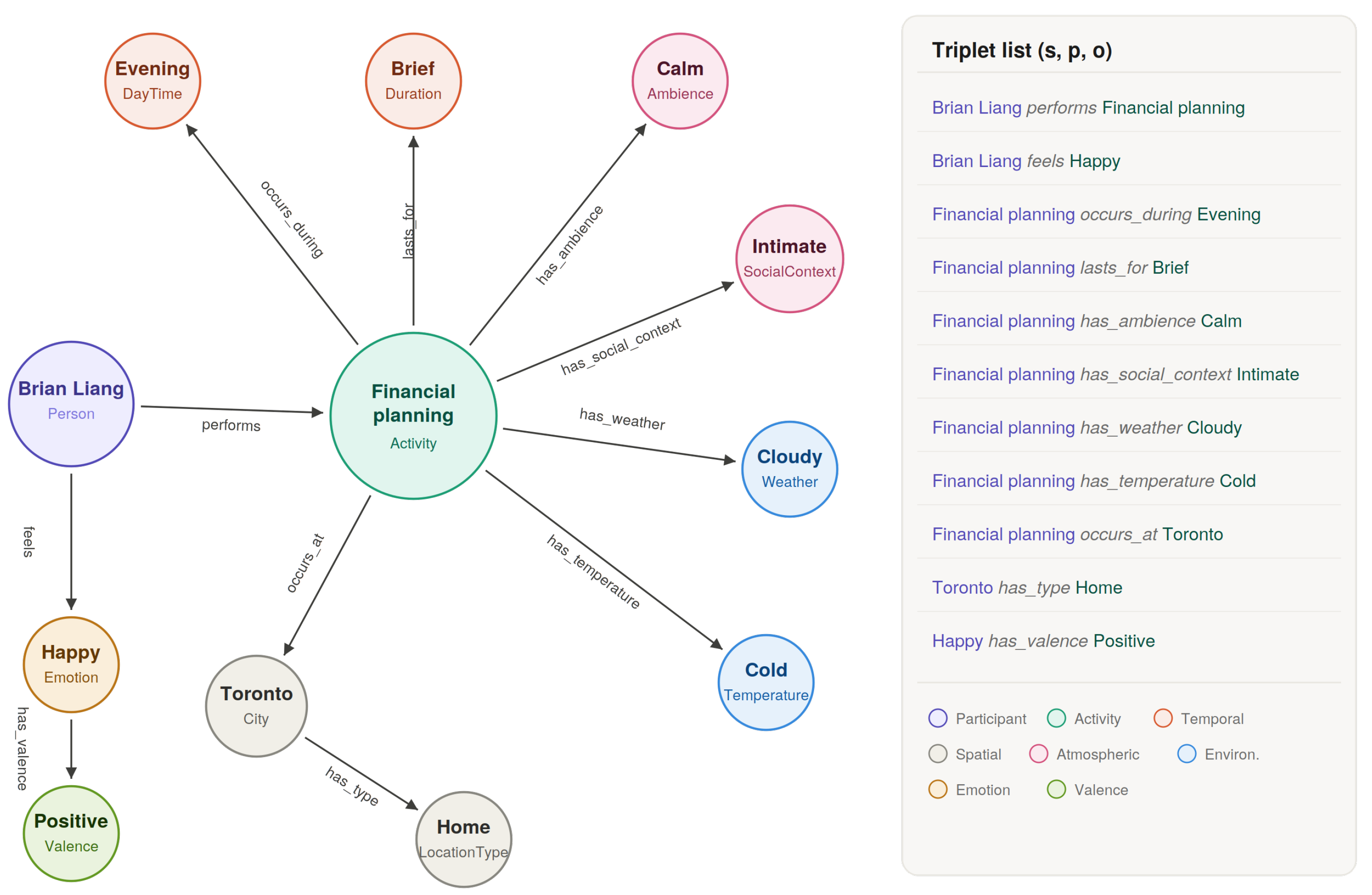
The Situation Graph is an ontology-aligned structured representation of the individual’s perspective at timestep t. Each is represented as a set of (subject, predicate, object) triplets . Each node carries a kind drawn from a fixed vocabulary of 13 semantic types (Table 1), an entity type drawn from a type-specific enumeration, and a free-text value populated by the autolabeler in Stage 6. The construction and structural validation of these relational representations builds conceptually upon recent advances in contextual scene graph generation [16], adapting visual-spatial grounding techniques to track latent psychological state.
Edges are drawn from 16 typed relations organized into five semantic groups: core action, spatiotemporal, atmospheric, environmental, and psychological (Table 2). A predefined constraint map specifies the valid source–target node-type pairs for each edge type. Table 2 provides the complete constraint map; a triplet is structurally valid if and only if . This rigid schema ensures that every generated graph is structurally valid (R4), providing explicit, ontology-grounded supervision for downstream perspective inference tasks.
Figure 3.
Example Situation Graph for a single timestep (Brian Liang, : financial planning). The left panel shows the graph structure with the Activity node as the central hub and typed edges radiating to spatiotemporal, atmospheric, environmental, and psychological nodes. The right panel lists all triplets comprising .
Figure 3.
Example Situation Graph for a single timestep (Brian Liang, : financial planning). The left panel shows the graph structure with the Activity node as the central hub and typed edges radiating to spatiotemporal, atmospheric, environmental, and psychological nodes. The right panel lists all triplets comprising .
4.2. Phase I: Persona Initialization (Stages 1–3)
Phase I defines and constructs the initial state of the simulated persona as well as the controlled event space from which future situations will be sampled.
4.2.1. Stage 1: Backstory Generation
Given a Persona Scaffolding , an LLM generates a coherent narrative backstory that integrates all eight scaffolding dimensions into a unified biographical text. The prompting strategy encourages three properties: (i) every scaffolding field must be incorporated, (ii) personality traits must be illustrated through concrete behaviors rather than abstract descriptions, and (iii) the narrative must maintain internal logical consistency across life chronology, relationships, and motivations. Because is synthesized entirely from without reference to real individuals, this stage satisfies privacy safety (R7).
A representative prompt for this stage is provided in Appendix A.1.
4.2.2. Stage 2: Event Taxonomy Loading
The Event Taxonomy is loaded from a static, versioned JSON specification containing 260 events across 14 categories. The taxonomy is a fixed, human-curated resource organized as a dictionary mapping category names to lists of specific events. This deterministic loading ensures full reproducibility (R6) and provides a controlled, auditable event space that supports systematic ablation over event categories (R1).
A representative filtering prompt is provided in Appendix A.2.
4.2.3. Stage 3: Initial Persona Matrix Extraction
The backstory is processed by an LLM to extract and synthesize the initial Persona Matrix . The LLM maps narrative elements to the fourteen schema clusters, quantifies traits on their defined scales (e.g., Big Five on , belief orientations on ), and infers reasonable values for underspecified attributes while maintaining internal consistency. The output is validated against the full typed schema to ensure all required fields are present, correctly typed, and within declared bounds (R4).
A representative system prompt for this extraction step is provided in Appendix A.3.
4.3. Phase II: Trajectory Simulation (Stages 4–5)
Phase II generates the latent longitudinal trajectory of the focal individual. Given the initial Persona Matrix and the event taxonomy , it constructs the Persona Path through sequential, state-conditioned simulation. This trajectory forms the structured backbone from which later labels and multimodal artifacts are derived.
To maintain coherence over long horizons, each timestep is generated through a validation-gated loop conditioned on the bounded history summary and cumulative narrative summaries. Stage 4 constructs the Persona Path itself, while Stage 5 derives a reusable registry of label values for subsequent Situation Graph generation.
4.3.1. Stage 4: Persona Path Generation
Stage 4 is the core simulation stage of PAiNT. It generates the full Persona Path through a multi-agent event-processing loop in which each timestep is gated by specialized validation agents. Rather than relying on a single prompt to produce an entire transition, the pipeline decomposes each event–reaction–update cycle into discrete substeps with independent validation. This modular design improves controllability and helps mitigate incoherence over long trajectories.
The generation pipeline processes T events sequentially using an EventProcessingAgent that orchestrates ten specialized sub-agents in sequence:
- 1.
- Category Selection: selects an event category from conditioned on recent history ;
- 2.
- Event Selection: samples a specific event from the selected category;
- 3.
- Time Selection: assigns a date and time within the simulation horizon;
- 4.
- Event Validation: rejects implausible events, near-duplicates within the recent history window, life-stage inconsistencies, or overrepresented categories;
- 5.
- Reaction Generation: produces the persona’s emotional and behavioral response conditioned on and ;
- 6.
- Reaction Validation: checks that the reaction is sufficiently specific, state-consistent, and temporally appropriate;
- 7.
- State Update Generation: proposes an updated Persona Matrix reflecting the impact of the event;
- 8.
- State Validation: enforces schema invariants, including constant-feature preservation and valid value ranges;
- 9.
- State Finalization: applies the validated state update;
- 10.
- Summary Generation: produces a natural-language summary of the transition for long-range context management.
4.3.1.1. Validation Protocol
Each generate–validate pair (steps 2/4, 5/6, 7/8) operates with a bounded retry mechanism of up to attempts per validation. For events, if all attempts fail validation, a deterministic fallback event (e.g., “daily routine”) with probability is auto-approved, guaranteeing completion. For reactions and state updates, the last attempt is accepted on exhaustion. This bounded retry protocol ensures that the pipeline always terminates (R3) while maintaining generation quality through multi-round refinement.
4.3.1.2. Context Management
At each step, generation is conditioned on the history summary (Eq. 4), , where k and m are configurable sliding-window sizes (default ). The sliding window keeps the structured state passed to each agent within a fixed token budget. To preserve long-range narrative context beyond this window, the Summary Generation sub-agent appends a natural-language summary after every state transition; the accumulated summaries are then passed alongside the windowed state to each agent, giving it access to the persona’s complete history without requiring the full sequence of structured Persona Matrices.
Representative event-selection and event-validation prompts are provided in Appendices Appendix A.4.1 and Appendix A.4.2, respectively; analogous prompts govern reaction generation, reaction validation, Persona Matrix update, and Persona Matrix validation within the same loop.
4.3.2. Stage 5: Label Extraction
Stage 5 derives a reusable registry of label values from the completed Persona Path. This registry is not itself a Situation Graph; rather, it is an intermediate structure used in Stage 6 to instantiate graph nodes with persona-consistent participants, locations, and activities. Its role is therefore to bridge the latent trajectory generated in Stage 4 and the ontology-aligned labels constructed in Phase III.
The pipeline is implemented as a three-node agent graph with a conditional loop:
- 1.
- Seed List Agent: extracts initial label values from and the backstory for five expandable node types: MainParticipant, Participant, Activity, Location, and LocationType.
- 2.
- Iterative List Agent: scans each pair in the Persona Path to identify additional label values from the event context (e.g., names of people involved, locations visited, activities performed).
- 3.
- List Verifier Agent: validates, merges, and deduplicates extracted values. A conditional edge routes back to Step 2 if ; otherwise the loop terminates.
The output is a typed dictionary that maps each node kind to its available grounded values (e.g., Participant ↦ {“Maya”: “Friend”, “Josh”: “Acquaintance”}). Stage 6 then uses this registry to populate Situation Graph nodes with consistent, trajectory-aligned identifiers.
4.4. Phase III: Artifact Generation (Stages 6–8)
Phase III converts the simulated latent trajectory into explicit perspective labels and observable multimodal artifacts. Given the Persona Path , this phase first constructs a Situation Graph for each timestep and then generates a corresponding set of artifacts . In this way, the latent state trajectory produced in Phase II is translated into labeled, partially observable digital footprints.
4.4.1. Stage 6: Situation Graph Generation
For each tuple in the Persona Path—where is the persona’s reaction to generated in natural language—Stage 6 produces a Situation Graph (Eq. 5) via a two-step process. First, an LLM extracts an unlabeled graph as a set of triplets, constrained to use only the 13 node types, 16 edge types, and valid source–target pairs defined by Table 2, with a maximum of 20 nodes per graph. Each graph must include at minimum a MainParticipant, Activity, Location, DayTime, Emotion, and Valence node.
4.4.1.1. Autolabeler
Second, an Autolabeler populates the value field of each node by selecting from the finite, persona-specific label registry produced in Stage 5. Recall that the label registry maps each expandable node kind to its set of grounded label values (e.g., ; ). Given the unlabeled graph produced in Step 1, the current Persona Matrix , and the event context , the Autolabeler selects the registry label that best fits each node’s role in the situation, grounding abstract node types to persona-consistent entities (e.g., mapping a Location node typed as City to “Toronto” rather than a generic placeholder). For closed-enumeration node types (Table 1), no autolabeling is required: the value is fully determined by the entity type .
This design plays a critical role in maintaining cross-timestep character coherence. Because every node value is drawn from the same shared label registry across all T timesteps, the Autolabeler enforces referential consistency: the same friend, location, or recurring activity is always denoted by the same canonical identifier throughout the trajectory. Without this mechanism, independently generated graphs could introduce synonymous but lexically distinct references to the same entity (e.g., “Maya” at vs. “Friend” at ), degrading entity co-reference and downstream artifact quality. In effect, the label registry acts as a persona-specific but trajectory-global controlled vocabulary, and the Autolabeler is the mechanism that binds each graph to it. This grounding propagates directly into Stages 7–8: because artifact specification and generation are conditioned on , the specificity and consistency of registry values determine whether the resulting text, image, and audio artifacts exhibit coherent, persona-differentiating content across the full simulation horizon.
A representative prompt for graph generation is provided in Appendix A.5.
4.4.2. Stage 7: Artifact Specification
Given , Stage 7 determines which artifacts should be generated for the current situation and with what parameters. Its purpose is to translate the latent state and structured perspective label into a concrete artifact-generation plan while preserving cross-modal alignment. This stage is implemented as a three-layer pipeline:
- Constraint Filtering: a Universal Constraints Agent applies both rule-based and LLM-based filters to eliminate implausible artifact types. Rule-based checks enforce behavioral plausibility, such as limiting posting frequency or rejecting image types that would be inconsistent with the situation. An LLM-based coherence check then verifies that each remaining artifact type is appropriate given and .
- Footprint Flow Construction: an LLM determines the set, ordering, and dependency structure of the artifacts to be generated for the current timestep, producing a structured generation plan
- Parameter Generation: for each selected artifact type, the pipeline generates detailed modality-specific parameters, such as recipients, tone, visual content, or audio characteristics, using validated typed schemas.
The candidate artifact pool spans 6 text types (email, text message, social media post, journal entry, search query, Twitter post), 6 audio types (phone recording, voicemail, conversation, voice memo, ambient soundscape, audio clip), and 3 image types (photo, phone photo, family picture).
4.4.3. Stage 8: Multimodal Artifact Generation
Modality-specific generators produce observable artifacts (Eq. 5), conditioned on the artifact parameters from Stage 7. The three modality generators execute as parallel tasks:
- Text: Email, text message, social media post, journal entry, and search query—generated via persona-aware structured prompting with first-person voice, natural hesitations, and typed output schemas.
- Audio: Voice memos, voicemails, conversation recordings, and ambient soundscapes—generated through a multi-agent pipeline (context analysis → script writing → tone initialization → voice design → audio effects → humanization) with a voice registry for speaker consistency and text-to-speech synthesis conditioned on emotional state. For soundscapes, the pipeline skips script writing, tone initialization, and voice design.
- Image: Photos and visual content—generated via text-to-image models with identity-consistent character embeddings derived from .
All modality generators receive a unified Situation State Description derived from , ensuring cross-modal consistency (R5). Artifacts are stored with rich metadata linking each item to its generative context , supporting full auditability (R6).
A representative text-modality system prompt is provided in Appendix A.6.
4.5. Implementation
PAiNT is implemented in Python with three core dependencies.
Prefect orchestrates the eight-stage pipeline as a directed acyclic graph of tasks: Stages 1→2→3→4 execute linearly; Stage 6 depends on Stages 1 and 4; Stage 7 depends on Stages 4 and 6; and Stage 8 depends on Stages 4, 6, and 7, with its three modality generators (text, audio, image) executing as parallel sub-tasks. Each Prefect task supports automatic retries (up to 2) and input-based caching for incremental re-runs.
LangGraph is used for multi-agent coordination in the stages that require conditional control flow. In particular, it supports the validation-gated event-processing loop in Stage 4 and the iterative label registry construction in Stage 5. Pydantic is used throughout the pipeline to enforce typed schemas and validate structured outputs.
The framework supports configurable LLM backends through a provider abstraction and exposes the main generation parameters through , including the random seed, temporal resolution, simulation horizon, and context window sizes . All generated outputs—including configurations, prompts, intermediate states, labels, and final artifacts—are persisted with provenance metadata, enabling reproducibility (R6) and controlled ablation studies (R1).
The full source code, documentation, and usage instructions are available in the project repository.
4.5.1. Downstream Task: Situation Graph Prediction
The paired data produced by PAiNT—multimodal artifacts alongside ontology-aligned Situation Graph labels —naturally supports the downstream task of Situation Graph Prediction (SGP): given observable artifacts from a single situation, infer the structured perspective representation that encodes the entity’s goals, affect, social context, and appraisal. In the PAi paradigm [13], SGP is an important supervised task because a sequence of predicted Situation Graphs can form the basis of a longitudinal Chronicle.
PAiNT’s contribution to SGP in this paper is as a data generator and benchmarking resource. By exposing as an explicit label with complete coverage within the simulation, PAiNT provides paired artifact–graph data intended to support future training and evaluation for SGP-style tasks. We demonstrate and evaluate a basic SGP pipeline on the downstream SGP task (Section 7.0.0.60), but defer measuring the transfer utility of the generated supervision to future work. A more detailed description of the released benchmark resource is provided in Section 7.
5. Metrics and Evaluation Protocol
We evaluate PAiNT using a metric suite designed to assess structural validity, temporal coherence, narrative consistency, and multimodal faithfulness. The metrics are organized into three families (Table 3): persona representation quality, which evaluates structural, temporal, and event-driven properties of the evolving Persona Path; distributional and stability diagnostics, which quantify inter-archetype separability, intra-archetype dispersion, and the geometry of identity trajectories in state-vector space; and data generation quality, which evaluates graph-level consistency and cross-modal alignment of generated artifacts.
Three design principles guide this suite. First, complementary coverage: each metric targets a failure mode not captured by the others, so the suite functions as an interlocking diagnostic rather than a collection of redundant scores. Second, requirement traceability: every metric operationalizes at least one of the design requirements R1–R7 (Section 3). Third, dual-role scoring: some metrics function as constraint-satisfaction checks, where violations indicate direct failures of the framework’s declared operating conditions, while others function as characterization diagnostics that support comparative analysis without defining a universal benchmark of realism. This distinction, used throughout Section 6, is critical for interpretation.
Within persona representation quality, we distinguish three sub-categories. Structural metrics verify that each generated Persona Matrix is well-formed with respect to the PAiNT schema (OCV). Temporal metrics evaluate how numerical attributes evolve across consecutive transitions: whether the trajectory respects the configured simulation horizon (THC), whether individual steps remain plausible (TSCD), whether sufficient cumulative change accrues over the full trajectory (TMD), and whether the distributional pattern of step-level drift activity resembles realistic human change rather than a mechanical or chaotic artifact (TVS). Event-driven metrics assess the quality and coherence of the event sequence itself: whether selected events are grounded in the canonical taxonomy (EQ) and whether the resulting narrative satisfies causal logic and semantic plausibility (NCNC).
5.1. Notation
Throughout this section, we assume a single identity with a single trajectory , as defined in Section 3. Each event is an evaluation unit.
For any metric score S, we use the following conventions:
- denotes the event-level score at timestep t.
- For any index set , the aggregated score over is .
- When the index set is the full trajectory, we write , and refer to S (without subscript) as the trajectory-level score.
When needed, we additionally use to denote the score for a single artifact of modality associated with event t.
5.2. Persona Representation Quality Metrics
This section introduces seven metrics—organized into structural (OCV), temporal (THC, TSCD, TMD, TVS), and event-driven (EQ, NCNC) sub-categories—that quantitatively evaluate the quality and coherence of evolving personas as represented through the Persona Matrix (Section 4). The Persona Matrix tracks both stable dimensions (e.g., ethnic background) and dynamic dimensions (e.g., stress level, work-life balance) that evolve as the persona experiences simulated events over time.
5.2.1. Ontology and Constraint Validity (OCV)
5.2.1.1. Question
Is every generated Persona Matrix structurally well-formed according to the PAiNT schema?
OCV is a structural prerequisite: it checks that every piece of data produced by the pipeline is valid with respect to the fundamental rules and constraints defined by the Persona Matrix schema. PAiNT applies OCV to two distinct data structures: the Persona Matrix (Stage 4) and the Situation Graph (Stage 6). For each structure, OCV verifies that all attributes conform to their respective schemas, as defined in Section 4.1.3 and Section 4.1.5 for the Persona Matrix and Situation Graph, respectively. If structural validity fails, no downstream metric can be trusted, because temporal, narrative, and distributional analyses all assume well-typed input. Since PAiNT generates data used to train graph-based machine learning models, it is critical that both the Persona Matrix structure and Situation Graph generated by PAiNT follow their pre-defined schema. OCV measures how well the data follows the desired structure quantitatively.
5.2.1.2. Design
In our implementation, OCV is evaluated by passing each data structure through the same Pydantic schema that PAiNT uses internally for validation. A structure that passes all schema checks receives a score of 1.0; a structure with k faulty attributes out of total receives a proportionally reduced score.
Formally, let be the sequence of Persona Matrices for the identity. Let be the total number of attributes in the schema, and let denote the count of attributes in that violate schema constraints. We define the OCV score for timestep t as:
The trajectory-level OCV is the average across all T timesteps:
5.2.1.3. Note
The two data structures exhibit qualitatively different OCV behavior, reflecting differences in their generation mechanisms. For Persona Matrices, PAiNT’s Stage 4 pipeline includes a self-regeneration mechanism that discards any matrix failing Pydantic validation and retries generation until it succeeds, guaranteeing by construction across all reported experimental conditions. We therefore treat Persona Matrix OCV as a pipeline guarantee rather than a differentiating experimental outcome. For Situation Graphs, no equivalent regeneration loop is applied in Stage 6, so OCV functions as a standard empirical metric.
5.2.2. Temporal Horizon Compliance (THC)
5.2.2.1. Question
Does the generated trajectory respect the specified simulation horizon, or is the generator overshooting or undershooting the target time window?
PAiNT is configured with an explicit simulation horizon (e.g., 365 days for a one-year simulation, 1,825 days for five years). A well-behaved generator should produce a Persona Path whose temporal span closely matches this target: a trajectory configured for one year should not terminate after three months (undershoot) or stretch to three years (overshoot). Unlike the other temporal metrics (TSCD, TMD, TVS), which evaluate the content of attribute transitions, THC evaluates the temporal scaffolding itself. Consequently, THC serves as a critical upstream diagnostic: because TSCD, TMD, and TVS scale their allowed drift budgets based on elapsed time, a generator that overshoots the horizon artificially inflates its allowed variance. THC ensures that fundamental temporal calibration failures do not appear falsely competitive on downstream metrics.
5.2.2.2. Design: Span Ratio and Coverage
Let denote the dates parsed from the Persona Matrices . We define the actual horizon as
clamped to a minimum of 1 day. The span ratio is:
THC combines two complementary sub-scores: a span score that penalizes deviations in total trajectory length, and a coverage score that penalizes events placed outside the nominal window.
5.2.2.3. Span Score
The span score evaluates the ratio r against an acceptable band using an asymmetric linear band-pass function (Eq. A3 in Appendix C). The asymmetry is deliberate: overshoot is penalized more aggressively than undershoot. A generator that undershoots by 50% receives a span score of 0.60—degraded but not catastrophic—while a generator that overshoots by receives a span score of 0.10, reflecting a fundamental failure of temporal control. Full parameterization and rationale are provided in Appendix C.
5.2.2.4. Coverage Score
The coverage score measures the fraction of Persona Matrices whose dates fall within the nominal simulation window :
A trajectory with places all events within the target window; a trajectory that overshoots will have because late events fall outside the window. Coverage complements the span score: a generator that concentrates most events within the target window but allows a few to spill over will receive high coverage but a reduced span score.
5.2.2.5. Final THC Score
The trajectory-level THC is a weighted combination of the two sub-scores:
where and . The higher weight on span reflects the primacy of total horizon compliance: a trajectory that covers the right timeframe is more valuable than one that merely keeps events within the window by truncating early.
5.2.2.6. Limitations
THC evaluates temporal extent but not temporal density: a trajectory that places 90 events in the first month and 10 in the remaining 11 months will score well despite exhibiting highly uneven event spacing. A dedicated event-spacing metric is a direction for future work.
5.2.3. Temporal Smoothness & Controlled Drift (TSCD)
5.2.3.1. Question
Are individual transitions between consecutive Persona Matrices plausible—i.e., do numerical identity attributes change at rates consistent with realistic human dynamics?
A person’s core traits and internal states should not change abruptly from one moment to the next. A persona whose stress level jumps from 1.0 to 5.0 between two events separated by three days, or whose Big Five openness shifts by two full points in a single step, is exhibiting implausible dynamics regardless of whether the schema is well-formed. TSCD detects such implausibly large per-step attribute changes, serving as a per-transition upper bound on the rate and magnitude of identity evolution.
5.2.3.2. Design: Rate Caps and Absolute Ceilings
For each monitored numerical attribute , we define two calibrated thresholds:
- A daily rate cap : the maximum plausible sustained change per elapsed day. This represents the rate that would be implausible to sustain across the full inter-event interval —it is not the maximum possible single-day fluctuation (which can be higher for volatile attributes like weight due to hydration effects), but rather the rate at which sustained drift becomes unrealistic.
- A hard absolute ceiling : the maximum allowable magnitude of change in a single transition, regardless of elapsed time. This acts as a secondary guard for long inter-event gaps where the rate check alone would become too permissive.
These thresholds are calibrated against the attribute scales defined in the Persona Matrix schema. For example, personality traits (OCEAN) are scored on a scale with a range of 4.0, while belief system attributes are scored on a scale with a range of 1.0. The rate caps are scaled proportionally so that the constraint strength (expressed as a fraction of the attribute’s total range) is comparable across all dimensions. The rate caps are grounded in published longitudinal data for personality traits, body weight, and perceived stress, then extended to remaining attributes by proportional scaling; the full derivation protocol and complete parameter table are provided in Appendix B (Table A1).
5.2.3.3. Attribute Set
We monitor fields spanning Big Five personality traits (5), weight (1), fitness (1), stress level (1), coping styles (5), work-life balance (1), nutritional habits (1), relational closeness (1, per relationship type), and belief system dimensions (5, on a scale). Three attributes are explicitly excluded: height (invariant for adults—any change is a schema error, not a drift violation), BMI (a derived field whose inclusion would double-penalize weight changes), and anxiety level (no bounded schema range is defined, making rate-cap calibration undefined). The complete monitored attribute set is listed in Appendix B.3.
5.2.3.4. Violation Criterion
For a transition from to with elapsed time days, the observed change in attribute a is , and the implied daily rate is . A violation is flagged when either:
or
Let be the set of attributes that trigger a violation at transition t, and let be the number of attributes successfully observed (i.e., present and numeric in both and ). The per-transition TSCD score is:
The trajectory-level TSCD is averaged over all transitions:
5.2.3.5. Elapsed Time Handling
The elapsed time is computed from the date fields of consecutive Persona Matrices, clamped to a minimum of 1 day to prevent division-by-zero in rate calculations. This clamping means that multiple events occurring on the same simulated day are evaluated under the strictest possible rate constraint, which is the desired behavior: sub-daily attribute fluctuations should be minimal.
5.2.3.6. Limitations
TSCD evaluates individual transitions in isolation. A trajectory in which every step is smooth but attributes never cumulatively change—generative stagnation—will receive a perfect TSCD score. This complementary failure mode is addressed by TMD (Section 5.2.4).
5.2.4. Temporal Macro Drift (TMD)
5.2.4.1. Question
Over the full trajectory, do state-like attributes accumulate meaningful change commensurate with the elapsed time, or is the persona generatively stagnant?
A trajectory can satisfy TSCD perfectly—every step small and smooth—yet produce a persona that barely evolves across hundreds of simulated days. This complementary failure mode is generative stagnation. A persona whose stress level, fitness, or relational closeness remains effectively unchanged over a simulated year is not exhibiting the expected dynamics of a realistic life trajectory, regardless of how smooth each individual step is. TMD detects this failure by measuring how much of the available drift budget each attribute actually consumed.
5.2.4.2. Design: Budget Utilization
For each state-like attribute a, the maximum available drift budget across the full trajectory is derived directly from the TSCD daily rate caps:
where is the daily rate cap (the same parameter used by TSCD) and is the elapsed time in days for transition t. The observed total variation is:
The utilization ratio is:
The min clamp handles the case where TSCD violations cause observed drift to exceed the rate-cap budget; such attributes have trivially consumed their full budget and receive no TMD penalty. A per-attribute score is then computed:
where is a minimum utilization threshold for attribute a. If a state-like attribute uses at least fraction of its available budget, no penalty is applied; otherwise, the penalty is proportional to the shortfall.
The trajectory-level TMD score is the weighted mean across all state-like attributes, where each attribute is weighted by the number of transitions for which it was successfully observed:
5.2.4.3. Attribute Classification: State-like vs. Trait-like
TMD intentionally restricts evaluation to state-like attributes—those for which stagnation is pathological. The monitored set includes: weight, fitness, stress level, work-life balance, nutritional habits, emotional reactiveness, and relational closeness (per relationship type). Trait-like attributes—Big Five personality traits, belief system dimensions, and most coping styles—are explicitly excluded from TMD. Stagnation in stable traits is not a failure; it is an expected property of realistic personas. The full classification rationale is provided in Appendix B.4.
5.2.4.4. Minimum Utilization Thresholds
Default thresholds are (5% budget utilization) for most attributes. Two exceptions are made: weight uses because its rate cap ( kg/day) yields a large absolute budget where 5% already represents non-trivial kilogram-scale movement; stress uses because it is the most volatile state-like attribute and a frozen stress trajectory is the clearest signal of generative stagnation.
5.2.4.5. Key Properties
TMD has several properties that distinguish it from simpler stagnation detectors such as a stall rate (the fraction of transitions with zero observed change): (i) it is continuous—no binary cliff from step-count thresholds; (ii) it is density-invariant— scales with actual elapsed days, so sparse and dense simulations are compared fairly; (iii) it inherits TSCD rate caps—a single shared parameter set ensures consistency, though this also means calibration errors are correlated; (iv) it is robust to epsilon gaming—cumulative total variation cannot be inflated by tiny per-step nudges without accumulating real movement.
5.2.4.6. Limitations
TMD measures the amount of cumulative change but not its distributional pattern across steps. A trajectory that concentrates all change in a single burst and then stagnates for the remaining steps may still satisfy TMD’s budget threshold. This distributional failure mode is addressed by TVS (Section 5.2.5).
5.2.5. Temporal Volatility Structure (TVS)
5.2.5.1. Question
Does thepatternof identity drift across timesteps exhibit the statistical texture of realistic human change—neither mechanically uniform nor chaotically erratic—and at a plausible overall activity level?
TSCD and TMD together bound individual-step and cumulative drift, but neither evaluates the distributional shape of drift activity across the trajectory. A generator that produces mechanically identical step sizes at every transition (uniform activity), or that alternates wildly between near-zero and maximal updates (erratic oscillation), satisfies both TSCD and TMD but fails to produce the naturalistic variability expected in real human change. TVS addresses this gap by characterizing the statistical structure of the step-level drift sequence.
5.2.5.2. Design: Normalized Step Utilization
For each transition t (comparing to with elapsed time days), we compute a normalized step utilization that expresses how much of the available TSCD rate budget was consumed at that step:
where is the subset of attributes successfully observed in both and , and is the TSCD daily rate cap for attribute a.
Intuitively, means nothing moved at step t; means every attribute simultaneously hit its TSCD rate ceiling; indicates TSCD violations (over-drift) at that step. The sequence encodes the full temporal activity profile of the trajectory.
5.2.5.3. Three Diagnostic Statistics
From the utilization sequence, we extract three statistics that characterize complementary aspects of distributional health.
(i) Mean utilization (): the overall activity level across the trajectory.
(ii) Coefficient of variation (): the distributional spread of activity across steps.
where is the sample standard deviation, and prevents division by zero.
(iii) Sequential jitter (): mean-normalized first-difference roughness, measuring step-to-step irregularity.
5.2.5.4. Band-Pass Scoring
Each statistic is evaluated against an acceptable band using a linear band-pass function:
where is the distance from the nearest band edge and is the penalty half-width controlling how rapidly the score decays outside the band.
The bands and penalty half-widths (all set to ) are:
| Statistic | Acceptable band | Penalty half-width |
| (MeanUtil) | 0.40 | |
| CV | 0.40 | |
| (Jitter) | 0.40 |
The band boundaries are motivated by the mathematical behavior of each statistic at its extremes. For , a value below implies near-complete stagnation: on average, fewer than 5% of the available drift budget is consumed per step, meaning the persona barely changes regardless of elapsed time. A value above implies that the trajectory sustains near-maximal drift continuously—as though every simulated period is one of extreme personal upheaval. For CV, a value below indicates that step-level activity is nearly uniform across the trajectory, a mechanical regularity inconsistent with the episodic nature of real human change; a value above indicates that activity is so unevenly distributed that a handful of steps account for almost all drift while the rest are effectively inert. For , a value below indicates that the activity level changes very smoothly from step to step—suggestive of a templated or deterministic generator rather than naturalistic variation—while a value above indicates wild oscillation between high and low activity at every transition. The penalty half-width is set to be comparable in magnitude to the band widths, ensuring scores decay gradually outside the acceptable range rather than dropping sharply at the boundary. In the absence of high-resolution longitudinal ground truth for identity drift, these bounds should be interpreted as heuristic guardrails rather than a calibrated realism baseline.
5.2.5.5. Final Score
Using the shorthands: , and , the TVS score is the equally weighted mean of the three band-pass scores:
Equal weighting reflects the fact that each statistic captures a distinct property: overall activity level, distributional spread, and sequential texture.
5.2.5.6. Attribute Set
TVS uses the same set of numerical attributes as TSCD (Section 5.2.3), with the same exclusions (height, BMI, anxiety level) and the same rate caps .
5.2.5.7. Limitations
The band calibration is empirical and may not transfer to substantially different simulation configurations (e.g., radically different temporal resolutions or persona schemas). We mitigate this by choosing wide bands and providing the band parameters as configurable inputs. Additionally, TVS evaluates drift patterns at the trajectory level and does not localize specific timesteps where the volatility structure degrades—it is a global diagnostic, not a per-step score.
5.2.6. Event Quality (EQ)
5.2.6.1. Question
Are the events sampled during trajectory generation grounded in the canonical Event Taxonomy, or is the generator hallucinating events outside the predefined catalogue?
PAiNT employs a controlled Event Taxonomy—a predefined catalogue of plausible life events organized into categories (Section 4.1.2). Even with Stage 2 loading and Stage 4 event validation, the event-selection step may still produce events whose names do not appear in this taxonomy. Such hallucinated events undermine the controlled event space on which later evaluation depends: if the event inventory is not stable, downstream metrics that rely on event semantics (e.g., NCNC prerequisite rules) may be operating on undefined or unintended inputs.
5.2.6.2. Design
Let denote the set of all event names in the canonical Event Taxonomy. EQ measures the fraction of trajectory events whose name appears in the taxonomy:
A score of 1.0 indicates that all sampled events are grounded in the taxonomy and no hallucination occurred.
5.2.6.3. Implementation
The canonical event list is stored as a JSON dictionary mapping category names to lists of event names. Event matching is performed by exact string comparison after whitespace trimming; no fuzzy matching is applied. This strict matching is intentional—it tests whether the generator produces events exactly as specified in the taxonomy, not merely events that are semantically similar.
5.2.6.4. Relationship to PAiNT Pipeline Stages
In the full PAiNT pipeline, Stage 2 (Event Taxonomy Loading) curates the event list and Stage 4 (Persona Path Generation) includes an Event Validation agent with retry logic. EQ therefore also functions as an end-to-end test of these validation mechanisms: a score below 1.0 indicates that the validation agents are failing to catch hallucinated events.
5.2.6.5. Limitations
EQ is a necessary but not sufficient condition for event quality. A taxonomy-grounded event may still be contextually implausible for a given persona (e.g., “Retirement” for a 20-year-old)—such semantic violations are the domain of NCNC (Section 5.2.7). Additionally, EQ does not evaluate the diversity or distribution of event selection within the taxonomy; a trajectory that repeatedly samples the same event would score 1.0 on EQ despite exhibiting generative monotony.
5.2.7. Narrative Coherence & Non-Contradiction (NCNC)
5.2.7.1. Question
Is the generated event timeline logically consistent and narratively plausible—free from causal violations, factual contradictions, and implausible sequences?
In PAiNT, the simulated event timeline must be both logically consistent and narratively plausible. A single evaluation mechanism is insufficient: rule-based systems can miss higher-level semantic incoherence, LLM-based audits may be variable, and pairwise NLI checks cannot capture global trajectory plausibility on their own. We therefore evaluate NCNC using three complementary components, each targeting a different class of failure.
5.2.7.2. Phase 1: Rule-Based NCNC
This component acts as a deterministic constraint checker, verifying that the sequence of events respects fundamental laws of causality (hard constraints). It applies a set of common-sense prerequisite rules—such as “Marriage” must occur before “Divorce” for the same partner, or “Job loss” cannot precede “Employment” at the same company—across the full sequence of T events. Each rule specifies a set of dependent patterns (events that require a precondition) and a corresponding set of prerequisite patterns (events that must have occurred earlier in the timeline). Matching is performed case-insensitively against event names and descriptions.
An event at time t is considered flagged if it matches a dependent pattern and no prior event matches the corresponding prerequisite. Let if event t is flagged, and 0 otherwise.
The complete prerequisite rule set is provided in Appendix D.
5.2.7.3. Phase 2: Attribute-Scoped NLI Contradiction Detection
While rules catch hard causal violations, they cannot detect factual contradictions within the generated content. This component uses a structured extraction and Natural Language Inference (NLI) pipeline to identify contradictions at the level of individual facts.
The pipeline operates in three stages: (1) Structured fact extraction: an LLM extracts atomic facts from each event as tuples , where categories are constrained to a fixed set (employment, location, relationship, education, financial, health, social, identity, habits); (2) Candidate identification: facts are grouped by and filtered for simultaneous contradictions (same timestep, different values) and unexplained reversions (), while facts at different timesteps with different values are classified as legitimate state transitions; (3) NLI confirmation: only the filtered candidate pairs are evaluated by a DeBERTa-v3-large cross-encoder NLI model [40], with a contradiction confirmed only at confidence threshold . Implementation details are provided in Appendix D.
Let be the set of timesteps implicated by any confirmed NLI contradiction. The NLI-based score is:
5.2.7.4. Phase 3: LLM-Based Semantic Audit
Neither rules nor pairwise NLI can assess global narrative plausibility—whether the overall arc of the persona’s life makes sense as a coherent trajectory. This component utilizes the semantic reasoning capabilities of an LLM, prompted with (i) the backstory and (ii) the observable event timeline. The LLM is instructed to identify five categories of issues: logical contradictions, causal violations, temporal impossibilities, character breaks, and repetition artifacts. It returns a set of issues, each with implicated event indices and a severity level in .
Let be the set of events implicated by any issue:
5.2.7.5. Combined NCNC Score
The three phase scores are combined as a weighted average:
where , , and . The weighting reflects relative confidence: rule-based checks are deterministic and noise-free; NLI checks are concrete but may contain model noise; LLM audits are the most expressive but also the most variable.
5.2.7.6. Design Rationale: Why Three Phases?
The three-phase design addresses a fundamental tension in narrative evaluation. Rule-based systems are precise but narrow—they can only check pre-specified patterns and miss emergent incoherence. NLI models can detect factual contradictions but lack temporal reasoning and cannot distinguish a legitimate state transition from a true contradiction without explicit scoping. LLM-based judges can reason holistically about narrative plausibility but are prone to hallucination and inconsistency, and their judgments are not reproducible. By combining all three, NCNC achieves coverage across hard logic (Phase 1), structured factual consistency (Phase 2), and soft semantic plausibility (Phase 3).
5.2.7.7. Limitations
The rule-based component is limited by the coverage of the prerequisite rule set; violations of rules not in will not be detected. The NLI component depends on the quality of structured fact extraction, which is itself LLM-generated and may miss or misclassify facts. The LLM audit is non-deterministic and may flag different issues across replicates. We mitigate this variability by running R independent replicates where feasible and reporting mean scores.
5.2.8. Identity State Vectorization for Distance-Based Analyses
To support clustering and distance-based diagnostics, each hierarchical Persona Matrix is mapped to a flat Identity State Vector. We construct by concatenating three sub-vectors:
where and each component draws from the Persona Matrix schema (§Section 4.1.3) as follows.
5.2.8.1. Core Psychology ()
This sub-vector concatenates three groups of continuous scalars, each linearly rescaled to : the Big Five personality traits (openness, conscientiousness, extraversion, agreeableness, neuroticism; originally ), five coping-style dimensions (avoidance, impulsivity, emotional reactiveness, emotional regulation, escapism; originally ), and five belief-system dimensions (existential, nihilist, humanism, stoicism, political leaning; natively , clamped).
5.2.8.2. Fixed Identity ()
Eight categorical fields are one-hot encoded under a shared column registry that fixes column order across all runs: income class, age group, work style, average sleep quality, communication style, handedness, eye color, and gender. The registry is seeded with all schema-defined enum values before any data is processed; free-text variants encountered at runtime (e.g., “woman” → “female”) are canonicalized before encoding. In the experiments reported here, .
5.2.8.3. Narrative ()
The persona’s life driver, long-term goals, and fears fields are concatenated into a single string and embedded with OpenAI text-embedding-3-large (dimension 3,072). The scaling factor prevents the high-dimensional embedding from dominating Euclidean distances: we set for t-SNE visualisation and for centroid-based analyses (Silhouette Score, Final-State Spread).
5.2.8.4. Design Note
By construction, the state vector captures identity-defining attributes—personality, demographics, beliefs, and goals—while deliberately excluding volatile state variables (stress level, fitness, weight, work–life balance) that evolve in response to events. The latter are separately evaluated by the temporal metrics TSCD and TMD (§Section 5.2.3–§Section 5.2.4). This separation ensures that the distributional diagnostics measure whether archetype identity persists across stochastic seeds, rather than whether transient state fluctuations happen to converge.
5.2.9. Inter-Class Separation: Silhouette Score
5.2.9.1. Question
Do distinct archetype priors produce separable regions in identity state space, or does the generator collapse different archetypes into overlapping clusters?
For each state vector belonging to archetype cluster , define the mean intra-cluster distance and the mean nearest-cluster distance :
where . The per-point silhouette score is:
and the overall silhouette score is the population mean:
Values near indicate tight, well-separated clusters; values near 0 indicate overlapping clusters; negative values indicate systematic misassignment.
5.2.10. Final-State Spread (Intra-Class Stability)
5.2.10.1. Question
Given the same archetype prior and generation configuration, do independent stochastic runs converge to consistent terminal identity states, or does randomness cause unbounded divergence?
For each archetype a with R independent runs, we compute the centroid of the terminal state vectors and the mean Euclidean distance to that centroid:
Lower indicates greater terminal-state consistency: stochastic event noise does not erase the archetype identity signal. Final-State Spread is reported per-archetype rather than aggregated, preserving diagnostic granularity for identifying which archetypes are most sensitive to stochastic variation.
5.3. Data Generation Quality
These metrics evaluate alignment between generated artifacts and their corresponding Situation Graphs. Unlike structural validity metrics, they are best interpreted diagnostically: they characterize coverage, groundedness, and contradiction patterns rather than defining a single normative target for realistic artifacts.
5.3.1. Situation Graph Entailment Consistency (SGC)
5.3.1.1. Question
Do generated artifacts entail the facts encoded in their corresponding Situation Graph, or do they omit or contradict ground-truth content?
SGC measures the extent to which generated artifacts reflect facts encoded in their corresponding Situation Graphs. For example, if the graph states that a person is jogging in a park with a friend, SGC evaluates whether the generated text, image, or audio is consistent with that content rather than omitting or contradicting it.
Let denote the set of modalities generated at event t, and let denote the set of fact triplets extracted from the Situation Graph . For each artifact and hypothesis triplet , let and be the NLI (Natural Language Inference) probabilities that artifact entails or contradicts hypothesis h. Define the artifact-level score:
The event-level SGC score is:
The final SGC is reported as the mean over all t.
5.3.2. Situation Graph Faithfulness (SGF)
5.3.2.1. Question
Are the facts asserted by generated artifacts grounded in the corresponding Situation Graph, or does the artifact introduce hallucinated or contradictory content?
While SGC measures coverage—whether the artifact reflects Situation Graph facts—it does not evaluate whether the artifact introduces unsupported or contradictory content. SGF addresses this complementary direction by reversing the premise–hypothesis relation: the Situation Graph serves as the premise, and artifact-extracted triplets serve as hypotheses. Intuitively, SGF measures the groundedness of the artifact: how much of what the artifact asserts is actually supported by the graph.
For each artifact , let denote the set of triplets extracted from the artifact and denote the label triplets from the Situation Graph . For each artifact-asserted triplet , a verdict is assigned using the same three-way classification as SGC: if the Situation Graph entails h, if it contradicts h, and if h is neither supported nor contradicted (ungrounded elaboration).
The artifact-level SGF score is:
This maps entailed triplets to , contradicted triplets to , and ungrounded triplets to —treating elaboration beyond the Situation Graph as neutral rather than penalizing it. The event-level SGF score is:
The final SGF is reported as the mean over all t.
5.3.2.2. SGC–SGF Complementarity
SGC and SGF form a complementary pair for cross-modal alignment. SGC asks whether the artifact covers the graph content; SGF asks whether the artifact remains grounded in that content. A high-SGC, low-SGF artifact covers the Situation Graph well but introduces substantial unsupported or contradictory material, whereas a high-SGF, low-SGC artifact is grounded but incomplete. Reporting both metrics helps distinguish omission failures from hallucination or contradiction failures.
5.3.2.3. Limitations
SGF’s treatment of “unknown” verdicts as neutral (score ) is a deliberate design choice that is agnostic about whether ungrounded elaboration is acceptable; a stricter variant could penalize unknowns more aggressively. Both SGC and SGF inherit limitations of the triplet extraction pipeline—facts the parser fails to extract are not evaluated.
6. Experiments
We evaluate PAiNT through five complementary experiments addressing three questions: (i) whether it generates longitudinal identity trajectories that preserve archetypal structure while still allowing controlled variation, (ii) which architectural components govern specific quality dimensions, and (iii) whether the resulting labels, artifacts, and runtime footprint are sufficiently coherent and practical for intended downstream use. The experiments probe five regimes: identity persistence, temporal robustness under horizon compression, architectural contribution, artifact–label alignment, and cost–quality trade-offs across backbone models.
Concretely, Experiment 1 tests whether trajectories remain archetype-consistent over time while preserving seed-level variability; Experiment 2 stress-tests temporal coherence under different horizon/resolution settings; Experiment 3 isolates the contributions of multi-agent orchestration and bounded-history conditioning through ablations; Experiment 4 evaluates the structural validity and semantic alignment of generated Situation Graphs and multimodal artifacts; and Experiment 5 examines computational and financial deployment cost across backbone models. Together, these experiments move from latent-state quality to observable-output quality and finally to operational feasibility.
Section 6.1 first defines the shared conventions used throughout the evaluation. Section 6.2, Section 6.3, Section 6.4, Section 6.5 and Section 6.6 then present the five experiments, each organized around a specific objective, compact setup, relevant metrics, and brief interpretation. Because the metric suite in Section 5 mixes constraint-satisfaction checks with characterization diagnostics, we report only the metrics that are analytically central to the claim under study.
6.1. Experimental Conventions
Before presenting the experiments, we clarify how the evidence in this section should be read. PAiNT is evaluated not as a single black-box predictor on a fixed benchmark, but as a controlled generative framework whose outputs must satisfy structural, temporal, narrative, and cross-modal requirements. Accordingly, different metrics play different epistemic roles: some verify whether the generator satisfies its declared constraints, while others characterize how it behaves under controlled changes in archetype, horizon, architecture, or backbone.
6.1.0.4. Evaluation Philosophy
The experiments are designed as structured stress tests rather than population-level statistical studies. Their purpose is to determine whether PAiNT behaves coherently under controlled manipulations, where it fails, and which components are responsible. This framing is especially important because long-horizon multimodal generation remains computationally expensive, making exhaustive large-scale hypothesis testing impractical at this stage. The results therefore provide controlled empirical evidence about framework behavior, not population-level effect estimates.
6.1.0.5. Score Interpretation
The metric suite in Section 5 contains two kinds of measurements. The first consists of constraint-satisfaction metrics, such as schema validity (OCV), taxonomy membership (EQ), horizon compliance (THC), and contradiction checks within narrative coherence (NCNC). For these metrics, high scores indicate compliance with explicit design requirements, while low scores indicate direct violations. The second consists of characterization metrics, such as volatility structure (TVS), temporal smoothness and controlled drift (TSCD), temporal macro drift (TMD), inter-archetype separation (Silhouette Score), intra-archetype terminal consistency (Final-State Spread), situation-graph consistency (SGC), and situation-graph faithfulness (SGF). These do not define a universal notion of correctness; instead, they characterize how the generator behaves across archetypes, horizons, ablations, or backbones. Throughout Section 6, we therefore distinguish between validity-style evidence and diagnostic evidence.
6.1.0.6. Common Configuration Settings
Unless otherwise stated, all experiments use the same PAiNT implementation and evaluation pipeline described in Section 4 and Section 5. We keep fixed the event taxonomy, Persona Matrix schema, Situation Graph ontology, and metric definitions, together with the same validation-gated generation protocol and logging infrastructure. When comparing archetypes, horizons, or architectural variants, non-target factors are held constant as much as possible. When comparing backbone models, prompts, schemas, and orchestration logic are likewise fixed so that differences reflect backbone behavior rather than prompt redesign.
6.1.0.7. Selective Metric Reporting
Not every metric is equally informative for every experiment. For example, inter-archetype separation is central to identity persistence but irrelevant to deployment cost, while horizon compliance is critical in temporal stress testing but secondary in artifact alignment. We therefore report only the metrics that are analytically relevant for the claim under study, and treat prerequisite invariants such as structural validity as such rather than as differentiating outcomes.
We follow this convention throughout the remainder of Section 6: each experiment isolates a specific question, reports the metrics most relevant to that question, and interprets them according to whether they function as hard validity checks or comparative diagnostics.
6.2. Experiment 1: Identity Persistence Across Archetypes
6.2.0.8. Objective
This experiment tests whether PAiNT’s identity initialization produces a durable archetype signal that persists above stochastic event noise over the full trajectory. We evaluate three claims: C1, transition-level stability, measured by TSCD (§Section 5.2.3); C2, inter-class separation in identity state space, measured by the Silhouette Score (§Section 5.2.9); and C3, terminal-state consistency across independent runs of the same archetype, measured by Final-State Spread (§Section 5.2.10).
6.2.0.9. Setup
We generate trajectories using GPT-5.2 for Stages 1–4. Four archetypes are evaluated: Reserved (Anika), Role Model (Brian), Self-centered (Danielle), and Average (Ethan), initialized from personality-cluster priors following Gerlach et al. [1]. All conditions share the same event pool with stochastic selection. For each archetype, we run seeds ( total runs), each with events over a one-year horizon. Occupation, age, location, and start year are held constant across conditions. For state-space analyses, each Persona Matrix is mapped to an Identity State Vector as defined in Section 5.
6.2.0.10. Evaluation Lens
We report only the metrics directly tied to the three claims: TSCD for transition-level stability (C1), Silhouette Score for inter-archetype separation (C2), and Final-State Spread for within-archetype terminal consistency (C3). Broader temporal and narrative diagnostics are deferred to experiment 3 (§Section 6.4).
6.2.0.11. Results
6.2.0.12. C1: Transition-Level Stability
The overall mean TSCD is (Table 5), indicating that most per-step updates remain within the calibrated drift bounds. Danielle shows the lowest TSCD (), consistent with a more volatile prior. The temporal profile in Figure 4 also reveals a clear warm-up effect: early transitions are less stable, while later transitions converge toward a higher and more stable regime. This pattern is plausible, as early events establish the trajectory and therefore induce larger state updates than later events that reinforce an already-formed identity.
6.2.0.13. C2: Inter-Class Separation
Archetype separation is moderate but persistent. The mean silhouette score is , with Danielle showing the strongest isolation () and Brian the weakest (). The t-SNE projection in Figure 6 shows that independent runs remain organized by archetype in identity state space rather than collapsing into a single mixed distribution. The Brian–Ethan overlap is clarified by the centroid decomposition in Table 4: their proximity is driven primarily by shared fixed demographic encodings rather than by a collapse of the psychological or narrative signal.
6.2.0.14. C3: Terminal-State Consistency
Terminal consistency is also supported. The overall mean terminal spread is (Table 5), with Ethan showing the tightest convergence () and Anika the widest spread (). Across timesteps, mean within-archetype spread remains below inter-archetype centroid distance (Figure 5), including at the terminal state. This indicates that stochastic runs of the same archetype converge to a bounded neighborhood while preserving separation from the other archetypes.
6.2.0.15. Interpretation
Taken together, the results support all three claims under the tested conditions. PAiNT produces trajectories that are predominantly smooth at the transition level, remain moderately separable across archetypes, and converge to archetype-consistent terminal neighborhoods despite stochastic event variation. The evidence should nevertheless be read as directional rather than inferential, since each condition uses only seeds and no formal significance testing is performed. The main conclusion is that archetype initialization remains strong enough to persist above stochastic noise while still allowing controlled within-archetype variation.
6.3. Experiment 2: The Longitudinal Stress Test
6.3.0.16. Objective
This experiment characterizes a coherence frontier: the trade-off between temporal resolution and simulation horizon when the same event count is distributed across different timescales. We evaluate four claims: C1, structural invariance across horizons; C2, resolution-dependent drift behavior; C3, systematic temporal-profile advantages for long-horizon configurations; and C4, narrative robustness in the rule-based and factual components of NCNC (§Section 5.2.7), together with archetype-specific vulnerability in the plausibility component under temporal compression.
6.3.0.17. Setup
All trajectories were generated with GPT-5.2 for Stages 1–4. We evaluate two archetypes—Danielle (highest drift volatility in Experiment 1, § Section 6.2) and Ethan (most stable terminal convergence)—under two horizon settings: 100 events over 100 days (short; approximately daily resolution) and 100 events over 5 years (long; approximately multi-week resolution). Each condition uses seeds, for 20 runs in total.
6.3.0.18. Evaluation Lens
We report the temporal and narrative metrics most central to the frontier hypothesis: OCV, TSCD, TMD, TVS, EQ, THC, a simple Composite score defined as their mean, and the three-phase NCNC breakdown (Rule, NLI, LLM, Combined; Table 8).
6.3.0.19. Results
6.3.0.20. C1: Structural Invariance
OCV is in all 20 runs, confirming that schema validity is preserved across both horizons and both archetypes under the current pipeline.
6.3.0.21. C2: Resolution-Dependent Drift
Temporal compression reduces local drift compliance, but not uniformly across archetypes. Short-horizon TSCD is lower than long-horizon TSCD for both Danielle () and Ethan (). However, Ethan’s short-horizon TSCD () remains higher than Danielle’s long-horizon TSCD (), indicating that archetype dynamics contribute at least as much as horizon setting to drift behavior.
6.3.0.22. C3: Temporal Profile
The strongest horizon effects appear in TVS and THC. For both archetypes, TVS increases sharply under the long horizon (Danielle: ; Ethan: ), while THC rises from a uniform in all short-horizon runs to at least in all long-horizon runs. By contrast, TSCD, TMD, and EQ change more moderately. This produces a clear composite advantage for long-horizon settings: Danielle improves from to , and Ethan from to (Table 6 and Table 7).
6.3.0.23. C4: Narrative Robustness
The NCNC results (Table 8) separate cleanly into robust constraint satisfaction and resolution-sensitive plausibility. The Rule and NLI components remain consistently high across all conditions (means ), indicating that causal prerequisites and attribute-level consistency are largely preserved under compression. The LLM component is more sensitive. Danielle shows a substantial drop under the short horizon (, std ), whereas Ethan degrades only modestly (, std ). The combined NCNC score therefore remains high overall, but its decomposition reveals that temporal compression disproportionately affects narrative plausibility for the more volatile archetype.
6.3.0.24. Interpretation
These results support what we call the coherence frontier: a multi-dimensional trade-off between temporal resolution, simulation horizon, and archetype volatility. Long-horizon configurations are systematically stronger, but the degradation is not uniform across metrics. As Figure 7 shows, the main penalties of temporal compression fall on TVS and THC, suggesting that volatility structure and horizon compliance are the most resolution-sensitive dimensions of the framework. At the same time, the comparison between Danielle and Ethan shows that archetype dynamics matter independently of resolution: the higher-volatility profile degrades more strongly in drift compliance and narrative plausibility under compression. The evidence should nevertheless be read as directional rather than inferential, since the experiment uses only two archetypes and seeds per condition. The main conclusion is that some quality dimensions remain relatively robust under compression, whereas others exhibit structural ceilings that sharply constrain short-horizon performance within the tested design space.
6.4. Experiment 3: Ablation Study—PAiNT vs. No-Agent vs. No-Memory
6.4.0.25. Objective
This experiment isolates the contribution of PAiNT’s two principal architectural components—multi-agent orchestration and sliding-window history conditioning—across four backbone LLMs. We evaluate four claims: C1, orchestration improves structural integrity and event validity; C2, history conditioning is critical for temporal realism; C3, backbone families exhibit different performance profiles rather than a single uniform ranking; and C4, THC (§Section 5.2.2) is a necessary upstream diagnostic because it reveals temporal calibration failures that other temporal metrics can obscure.
6.4.0.26. Setup
We compare three variants: PAiNT (full pipeline), No-Agent (single-pass generation with history retained but no validation/retry), and No-Memory ( with orchestration retained). Four backbones are evaluated: GPT-5.2, GPT-4o, DeepSeek-V3, and Qwen3-235B-A22B-Instruct. This yields 12 conditions with seeds each (60 runs total), all at events over a one-year horizon. A single archetype, demographic assignment, and event taxonomy are held fixed to isolate architectural and backbone effects.
6.4.0.27. Evaluation Lens
We report the metrics most relevant to the ablation claims: EQ, TSCD, TMD, TVS, THC, and the NCNC decomposition (Rule, NLI, LLM). We also report a Temporal composite defined as the mean of TSCD, TMD, TVS, and THC; the NCNC composite defined as the weighted average in Equation (29) (); and an Overall Composite that aggregates Temporal, EQ, and NCNC.
6.4.0.28. Results
6.4.0.29. C1: Structural Integrity and Event Validity
The results support the claim that orchestration is the primary driver of event validity and a major driver of structural reliability under the reported metrics (Figure 8). Under the full PAiNT pipeline, EQ remains near-perfect across all four backbones (, with for GPT-5.2, GPT-4o, and Qwen3), whereas removing orchestration causes the largest degradation, especially for open-weight models. The clearest case is Qwen3, where EQ drops from under PAiNT to under No-Agent. Proprietary backbones are more robust under ablation (No-Agent EQ ), but still degrade relative to the full system. A similar pattern appears in narrative plausibility: DeepSeek’s NCNC falls to without agents, but recovers to under PAiNT. By contrast, NCNC and NCNC remain near ceiling across all conditions, suggesting that low-level causal and factual consistency is comparatively robust, while open-ended narrative plausibility benefits more directly from orchestration.
6.4.0.30. C2: History Conditioning for Temporal Realism
Removing memory degrades temporal realism most clearly in TVS and, in some cases, THC. For GPT-5.2, TVS drops from under PAiNT to under No-Memory. The most severe failure occurs for Qwen3, where No-Memory yields THC , corresponding to a severe horizon overshoot. These results indicate that history conditioning is especially important for maintaining naturalistic volatility structure and temporal frame awareness, even when the validation loop is preserved.
6.4.0.31. C3: Backbone-Dependent Profiles
The backbones do not differ by a single scalar notion of quality; instead, they exhibit distinct performance profiles. Proprietary models occupy the top two composite scores under the full pipeline, led by GPT-5.2/PAiNT at and GPT-4o/PAiNT at (Table 9). At the same time, open-weight models remain competitive in selected dimensions: DeepSeek/PAiNT achieves the highest TMD (), and Qwen3/PAiNT achieves perfect scores on EQ, NCNC, and NCNC. The main divergence is temporal: the open-weight models tend to combine strong cumulative drift with weaker smoothness or volatility structure, producing less balanced temporal profiles overall.
6.4.0.32. C4: THC as Upstream Diagnostic
THC exposes calibration failures that would otherwise remain partially hidden (Figure 8). Without THC, Qwen3/No-Memory would appear mid-tier on TSCD, TMD, and TVS alone; once THC is included, its temporal score drops to because those scores were achieved over a severely expanded horizon. The same logic applies to DeepSeek/PAiNT, whose high TMD () is partly offset by horizon overshoot (THC ). THC also clarifies the mechanism of single-pass failure: No-Agent settings do not merely degrade slightly, but often collapse chronologically, with GPT-4o, DeepSeek, and Qwen3 all showing catastrophic THC values near –. This indicates that orchestration is not only a quality enhancer, but also a practical requirement for maintaining long-range temporal pacing.
6.4.0.33. Interpretation
Taken together, the ablation results show that PAiNT’s two core components govern different quality dimensions. Multi-agent orchestration is the stronger guardrail for event validity, narrative plausibility, and chronological pacing, whereas history conditioning is particularly important for temporal realism and volatility structure. Across the four backbones, retaining orchestration (No-Memory) yields a higher composite score than retaining memory alone (No-Agent) in three of four cases, with the fourth showing only a small gap. This pattern suggests that active validation is the higher-priority architectural component overall, although the evidence remains directional because the ablations also alter prompt structure and generation flow. More broadly, the experiment shows that backbone choice should be driven by the specific quality dimension required for the downstream task: proprietary backbones are more balanced overall, while open-weight models can remain competitive in narrower dimensions under the full PAiNT architecture.
6.4.0.34. Limitations
These results are informative but should be interpreted while understanding their caveats. First, each condition uses seeds, so point estimates may retain non-trivial variance. Second, the ablation variants differ not only in the targeted component but also in prompt structure and generation flow, which weakens causal attribution. Third, the TVS band-pass parameters were calibrated on proprietary-model behavior and may partially disadvantage open-weight backbones. Fourth, the experiment uses a single archetype and a one-year horizon, so the observed interactions may not fully generalize. Finally, NCNC relies on a single LLM judge without inter-judge agreement analysis.
6.5. Experiment 4: Situation Graph Alignment and Artifact Faithfulness
6.5.0.35. Objective
This experiment evaluates whether, given validated Persona Paths, the downstream pipeline (Stages 5–8) produces structurally valid Situation Graphs and artifacts that remain meaningfully aligned with those graph labels. We evaluate three claims: C1, generated Situation Graphs achieve majority schema compliance, with violations attributable primarily to the graph-generation process rather than to archetype identity; C2, artifact label coverage follows a modality hierarchy, with modality exerting a stronger effect than archetype; and C3, artifact-asserted facts are more often ungrounded elaborations than outright contradictions, with text artifacts achieving the strongest entailment.
6.5.0.36. Setup
For each of the four archetypes from Experiment 1 (§ Section 6.2), we select the Persona Path closest to the archetype centroid as fixed input to Stages 5–8. We then generate seeds per archetype (20 runs total). GPT-5.2 is used for Situation Graph construction (Stage 6) and text artifact generation; triplet extraction for text, image, and audio transcript is performed using Gemini 3 Pro. Artifacts span text (emails, messages, journal entries, social media, search queries), image (photos, visual content), and audio (voice memos, ambient soundscapes).
All SGC and SGF scores are computed only for steps whose Situation Graph passes schema validation with OCV . On average, 39.3 of 50 steps per run satisfy this threshold, yielding approximately 786 evaluated steps across the 20 runs. As an instrument check, we also evaluate an NLI self-entailment ceiling using identical premise–hypothesis triplets. Across all 1,000 steps, mean self-SGC/self-SGF is , implying that roughly 3.5 percentage points of measured deficit are attributable to instrument limitations rather than generation quality alone.
6.5.0.37. Evaluation Lens
We report three classes of evidence: OCV for graph structural validity; SGC for label coverage, that is, how much graph content is reflected in the artifact; and SGF for groundedness, that is, how much of what the artifact asserts is supported by the graph. These metrics are diagnostic rather than normative: perfectly maximal SGC or SGF would imply unrealistically tight coupling between a compressed Situation Graph and a naturalistic artifact. In practice, the more informative failure modes are low SGC, which indicates weak conditioning on the graph, and high contradiction rates in SGF, which indicate active hallucination or conflict.
6.5.0.38. Results
6.5.0.39. C1: Graph Structural Validity
Situation Graphs achieve majority schema compliance. Mean OCV is overall (Table 10), indicating that most graph attributes are structurally valid, though the residual error rate remains non-trivial. Scores are tightly clustered across archetypes (range: –), supporting the claim that the violations arise primarily from the graph-generation process rather than from archetype-specific difficulty. This identifies Stage 6 as a current structural bottleneck: graph generation would likely benefit from stronger post-hoc validation or a regeneration mechanism analogous to the one used for Persona Matrices in Stage 4.
6.5.0.40. C2: Label Coverage Follows a Modality Hierarchy
A clear modality ordering emerges in SGC (Table 11): text achieves the highest coverage (), followed by audio (), then image (). This ordering is consistent across archetypes, while archetype-to-archetype variation per modality remains comparatively small (Text: –; Image: –; Audio: –). The evidence therefore supports the claim that modality is the dominant predictor of coverage. Danielle tends to score slightly lower than the other archetypes across modalities, but the effect is modest relative to the modality gap itself.
6.5.0.41. C3: Groundedness Is Limited More by Elaboration Than By Contradiction
The same modality ordering appears in SGF (Table 12): text achieves the highest groundedness (), while image () and audio () are lower and nearly tied. The verdict distribution in Table 13 provides the clearest interpretation: the dominant category is non-entailment without contradiction (59.2%), whereas negative entailment accounts for 18.4% of artifact triplets overall. Text achieves both the highest entailment rate (31.3%) and the lowest contradiction rate (15.3%), while image exhibits the highest contradiction rate (20.9%). These results support the claim that the main gap is not direct conflict with the Situation Graph, but elaboration beyond what the graph encodes. In that sense, the absolute SGF score should be interpreted together with the verdict composition rather than in isolation.
6.5.0.42. Interpretation
Taken together, the results suggest that the downstream pipeline is already a useful graph-conditioned artifact generator, but its quality is shaped by two different bottlenecks. The first is structural: Situation Graph generation achieves only moderate OCV, and this limits how many steps can be evaluated downstream. The second is modality-dependent grounding: text artifacts are consistently the most aligned and grounded, whereas image and audio artifacts contain more information that falls outside the graph or is harder to recover reliably through triplet extraction. The positive SGC–SGF association in Figure 9 indicates that these are not competing objectives in the present setup: better artifacts tend to be both more comprehensive and more grounded. The evidence should nevertheless be read as diagnostic rather than inferential, since each archetype uses only seeds and the NLI-based measurement pipeline itself has a ceiling below 1.0. The main conclusion is therefore not that artifact fidelity has been solved, but that the current pipeline is already informative enough to localize the dominant structural and modality-specific bottlenecks.
6.5.0.43. Limitations
These results are informative, but we note some caveats that should be considered. First, the Situation Graph label space is uneven: emotionally positive latent labels are overrepresented, which may make some hypotheses easier to entail than more specific surface-level facts. Second, with seeds per condition, per-archetype SGC and SGF estimates retain non-trivial variance. Third, the NLI measurement ceiling of implies that a small portion of the observed score deficit is attributable to instrument limitations rather than generation quality. Finally, both SGC and SGF inherit limitations from the triplet extraction pipeline. In particular, facts not extracted are not evaluated, and SGF’s neutral scoring of “unknown” verdicts is one of several defensible choices—stricter alternatives that penalize ungrounded triplets would shift absolute SGF values, but not the cross-modality and cross-archetype comparisons our findings rely on.
6.6. Experiment 5: Cost–Quality Trade-Offs
6.6.0.44. Objective
This experiment evaluates the operational cost of deploying PAiNT and relates that cost to the quality patterns established in Experiments 3–4 (§ Section 6.4Section 6.5). We focus on two questions: first, how the four backbone models compare in monetary cost and wall-clock time for the core persona simulation phase (Stages 1–4); and second, how resource demands scale when the full PAiNT pipeline (Stages 1–8) is executed end-to-end with the highest-performing backbone.
6.6.0.45. Setup
Cost estimates are derived from the mean per-run token counts observed in our experiments for trajectories of events with seeds. Backbone comparison uses the full PAiNT configuration from Experiment 3 (§ Section 6.4) for Stages 1–4. Full-pipeline scaling is measured from 20 complete GPT-5.2 runs spanning Stages 1–8. Prices reflect the API endpoints used in our experiments as of April 2026 and exclude caching discounts, bulk-rate agreements, or infrastructure-specific optimizations.
6.6.0.46. Evaluation Lens
We report input tokens, output tokens, estimated USD cost, and wall-clock time. Cost is interpreted jointly with the quality evidence from Experiment 3 (§ Section 6.4): the main issue is not simply which model is cheapest, but which model offers the most useful balance between quality, cost, and latency under the full PAiNT architecture.
6.6.0.47. Results
6.6.0.48. Backbone Comparison for Stages 1–4
Table 14 summarizes the estimated per-run cost of the core simulation phase under the full PAiNT configuration, while Table 15 provides the corresponding token and runtime footprint across architectural variants. The cost landscape separates into three broad tiers. Qwen3 is the least expensive backbone at $1.25 per run, followed by DeepSeek-V3 at $4.00, GPT-4o at $7.99, and GPT-5.2 at $11.01. These differences are driven not only by token volume but also by provider-specific pricing structure: Qwen3 remains inexpensive despite high token consumption, whereas GPT-5.2 and GPT-4o incur substantially higher output-token costs.
Cost does not align monotonically with quality. GPT-5.2 delivers the strongest overall performance under the full PAiNT pipeline (Composite in Experiment 3, § Section 6.4) but at the highest monetary cost. GPT-4o provides the second-best quality (Composite ) at 27% lower cost and less than half the wall-clock time. At the other extreme, Qwen3 is the most economical option but shows substantial weaknesses in temporal realism, particularly on TVS. This confirms that deployment decisions should be guided by the specific quality floor required by the downstream use case rather than by cost alone.
6.6.0.49. Architectural Overhead
Table 15 also clarifies the cost of PAiNT’s architectural safeguards. Across all four backbones, the full PAiNT pipeline requires substantially more tokens and time than either No-Agent or No-Memory. For example, GPT-5.2/PAiNT consumes 3.34M input tokens and 95.1 minutes per run, compared with 0.55M input tokens and 26.0 minutes for GPT-5.2/No-Agent. Similar gaps hold across the other backbones. This overhead is the operational price of the quality gains identified in Experiment 3(§ Section 6.4): orchestration and history conditioning improve structural integrity and temporal realism, but they do so by substantially increasing interaction depth and runtime.
Figure 10.
Cost–quality trade-off across backbones and architectural variants (Stages 1–4, events, seeds per condition). Cost is estimated from mean per-run token counts at API rates as of April 2026.
Figure 10.
Cost–quality trade-off across backbones and architectural variants (Stages 1–4, events, seeds per condition). Cost is estimated from mean per-run token counts at API rates as of April 2026.
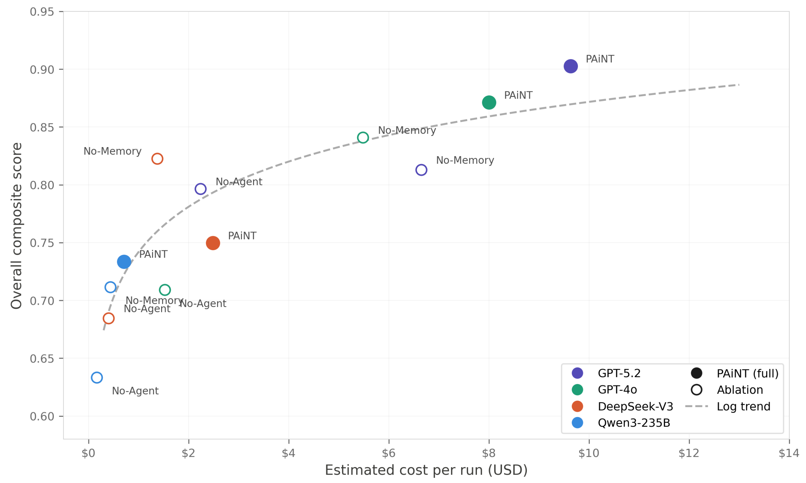
6.6.0.50. Full-Pipeline Scaling (Stages 1–8)
To estimate end-to-end deployment cost, we executed 20 complete PAiNT runs using GPT-5.2, the highest-performing backbone in Experiment 3 (§ Section 6.4). As shown in Table 16, the full pipeline consumes on average 5.56M input tokens and 0.66M output tokens per persona, for a mean cost of $19.01 and a mean wall-clock time of 210.1 minutes. Relative to the Stages 1–4 baseline, this corresponds to roughly 66% more input tokens, 80% more output tokens, and more than a doubling of elapsed time per run. At this scale, generating a dataset of 100 complete persona trajectories would cost approximately $1,901 before parallelization or optimization.
6.6.0.51. Interpretation
Taken together, the cost results show that PAiNT is already practical for controlled research-scale generation, but still expensive enough that deployment choices must be metric-aware. GPT-5.2 serves as the highest-quality reference configuration, whereas GPT-4o appears to be the strongest practical compromise between quality, speed, and monetary cost. Open-weight backbones offer substantial savings, but those savings are meaningful only if the resulting trajectories satisfy the structural and temporal quality floors required by the intended downstream use case. More broadly, these results confirm that PAiNT’s architectural improvements are not free: validation and memory materially increase runtime and token consumption, so the framework should be configured according to whether the target application prioritizes maximum quality, lower cost, or faster iteration.
6.6.0.52. Limitations
These estimates are deployment-specific and should be interpreted accordingly. They depend on the API endpoints, pricing schedules, and inference settings used in our experiments, and therefore may change over time or under other providers. The analysis also excludes volume discounts, prompt caching, batching strategies, and parallel execution effects, all of which could materially change effective cost. Finally, the cost projections for open-weight backbones are meaningful only insofar as the corresponding models satisfy the quality floors required by the downstream task; a cheaper configuration is not useful if it fails the structural or temporal constraints established earlier in Section 6.
7. PAi-Bench
We release PAi-Bench, a curated benchmark resource generated by PAiNT and reviewed by a human expert, designed to support future evaluation of longitudinal perspective-inference systems. This section documents its composition, structural properties, thematic diversity, modality distribution, curation protocol, intended downstream use, and reproduction cost.
7.0.0.53. Composition
PAi-Bench comprises four persona trajectories—Anika (Reserved), Brian (Role Model), Danielle (Self-centered), and Ethan (Average)—each spanning 100 causally ordered events over approximately two years of simulated time (January 2015 to February 2017). The four personas share a fixed demographic profile (age 22, Toronto, early-career management/consulting analyst, university degree, low–middle income). Each archetype is anchored to one quadrant of the four-way Big Five typology of Gerlach et al. [1], and the released trajectory for each archetype was selected as the Persona Path closest to its archetype centroid in state-vector space, using the centroids computed in Experiment 1 (§ Section 6.2).
To amortize the cost of long-horizon generation, the 100 events per persona were produced as two contiguous 50-event halves. The second half resumes generation from the exact state reached at the end of the first: the Persona Matrix , the partial Persona Path , and the bounded history window are loaded as initial conditions for step . Because the update rule depends only on the immediately preceding state and bounded history, this two-stage execution is operationally equivalent to a single run under the state-conditioned dynamics of PAiNT, differing only in sampling stochasticity. The merged Persona Path is the released object.
Each situation is paired with one ontology-aligned Situation Graph and three observable artifacts: one text artifact, one audio artifact, and one image artifact. In total, PAi-Bench contains 400 situations, 400 Situation Graphs, and 1,200 observable multimodal artifacts across the four personas. This organization is important for downstream use: each event provides dense, per-situation graph supervision together with aligned multimodal observations.
7.0.0.54. Situation Graph Structure
Because every artifact in PAi-Bench is supervised by an ontology-aligned Situation Graph, the structural richness of those graphs directly affects the benchmark’s value for Situation Graph Prediction (§Section 4.5.1) and related auditing tasks. Table 17 summarizes the distribution of unique nodes per graph across the four trajectories. All 400 graphs comply with the schema constraints of Table 1 and Table 2: every graph contains the six required node kinds (MainParticipant, Activity, Location, DayTime, Emotion, Valence) and respects the typed edge constraint map. The overall mean is unique nodes per graph (SD across archetypes ). Figure 11 shows that the benchmark graphs contain a stable core of required spatiotemporal and affective relations, while social and psychological predicates appear more selectively, reflecting their conditional role in the ontology.
Node values are drawn from the persona-specific label registry produced in Stage 5 (§Section 4.3.2), which guarantees trajectory-global referential consistency: the same friend, workplace, or recurring activity is denoted by the same canonical identifier across all 100 events of a given persona. The expanded label registries are of comparable size across archetypes, with on average 32 Participant labels, 18 Location labels, and 11 LocationType labels per persona. Figure 12 further shows that the required node types occur in nearly all graphs, while optional node types such as Participant vary more substantially across situations, making the benchmark structurally consistent but still non-trivial for downstream graph inference.
7.0.0.55. Event Coverage and Thematic Diversity
The 400 situations in PAi-Bench draw from 80 distinct event titles in the PAiNT event taxonomy (§Section 4.1.2), with each archetype covering between 47 and 55 unique titles (Anika: 55, Brian: 51, Danielle: 47, Ethan: 47). Figure 13 shows the 15 most frequent event titles across all four personas. The distribution is heavy-tailed: a small core of broadly shared life events (Acute injury, Achieving career goals, Experiencing workplace conflict, Learning a new skill, Financial planning) appears across all archetypes, while the long tail captures archetype-specific behavior—for example, Managing anxiety concentrates in Danielle (5 occurrences; absent in Ethan, elsewhere), Taking out a loan concentrates in Danielle (5 vs. elsewhere), Dental correction appears only for Anika (6), and Financial anxiety appears only for Ethan (4). This combination of a shared thematic core with archetype-specific divergence is what makes PAi-Bench suitable both for within-archetype longitudinal tracking and for across-archetype contrastive evaluation. The full rank-frequency distribution is shown in Figure 14.
7.0.0.56. Artifact Modality Breakdown
The 1,200 observable multimodal artifacts are distributed as follows. Text artifacts (400) are dominated by short-form messages () and journal entries (), with emails () and social media posts () making up the remainder. Audio artifacts (400) are predominantly voice memos (), followed by conversation recordings (), voicemails (), phone recordings (), and ambient/video-derived clips (). Image artifacts (400) are mostly point-of-view shots (), with selfies (), group photos (), and one screenshot rounding out the set. The strong skew toward first-person perspectives (voice memos, POV images, journal entries, SMS) reflects the design goal of producing artifacts that a real user would plausibly originate themselves, consistent with the longitudinal digital-footprint framing of PAi.
Figure 15.
Artifact modality distributions across the 400 situations in PAi-Bench. Audio artifacts (left) are dominated by voice memos (); text artifacts (center) skew toward short-form messages () and journal entries (); image artifacts (right) are overwhelmingly point-of-view shots (). The first-person skew across all three modalities is intentional and reflects the design goal of modeling artifacts that a real user could plausibly originate over time.
Figure 15.
Artifact modality distributions across the 400 situations in PAi-Bench. Audio artifacts (left) are dominated by voice memos (); text artifacts (center) skew toward short-form messages () and journal entries (); image artifacts (right) are overwhelmingly point-of-view shots (). The first-person skew across all three modalities is intentional and reflects the design goal of modeling artifacts that a real user could plausibly originate over time.
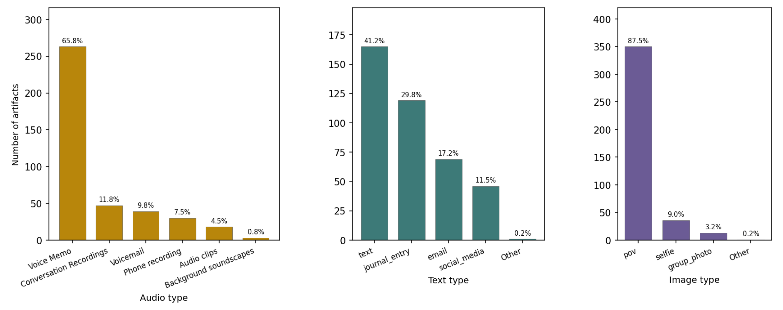
7.0.0.57. Curation and Human Validation
While PAiNT substantially accelerates and structures the dataset generation process, it should be treated as an assistive tool rather than a fully autonomous pipeline, as LLM-based generation can introduce subtle errors that automated validation alone does not catch. Failure cases encountered during manual review included incorrect or inconsistent event dates embedded in artifact content (e.g., text messages or journal entries referencing dates outside the simulated window), which aligns with the temporal calibration failures observed experimentally—particularly the horizon overshoot patterns identified by the THC metric. Each generated event was manually inspected for narrative plausibility, artifact–graph alignment, and factual consistency with the persona’s simulated state; image artifacts were additionally reviewed for visual faithfulness to their corresponding Situation Graph, with non-conforming images flagged and re-rendered through a refinement pass (111 of 400, or 27.8%, were regenerated in this way for improved quality). Events flagged for causal violations or schema inconsistencies at earlier automated stages were likewise regenerated until passing both automated checks and human review. Taken together, this human-in-the-loop curation layer is an essential complement to PAiNT’s automated validation, ensuring that PAi-Bench meets a quality standard suitable for meaningful downstream evaluation.
This curation protocol does not eliminate all benchmark limitations, but it provides an important quality-control layer beyond the automated generation pipeline alone. In particular, it reduces obvious visual mismatches and narrative breakdowns that would otherwise make downstream evaluation less meaningful.
7.0.0.58. Reproduction Cost
Table 18 reports the wall-clock time, token consumption, and LLM-only API cost required to regenerate each trajectory end-to-end with GPT-5.2 as the backbone. Across the four personas, PAi-Bench was produced in 27.8 wall-clock hours using 44.96M input tokens and 5.25M output tokens, for a total LLM-only cost of approximately $152, or $0.38 per labeled situation. These figures exclude non-token API charges for image generation and audio synthesis, which are billed per asset rather than per token. Consistent with the trend reported in Experiment 5 (§ Section 6.6), cost scales sub-linearly with trajectory length because bounded-window history conditioning prevents prompt size from growing linearly with the event index.
7.0.0.59. Intended Use and Current Scope
PAi-Bench is designed to support two downstream tasks: (i) Situation Graph Prediction (§Section 4.5.1), in which a model must infer the structured perspective representation from raw multimodal artifacts, and (ii) longitudinal identity tracking, in which a model must detect how identity state evolves across an event sequence. Because every situation is paired with an explicit Situation Graph and generated from a known Persona Matrix state, PAi-Bench provides dense, per-situation supervision that is unavailable in real-world digital-footprint datasets.
In this paper, however, PAi-Bench is introduced as a released benchmark resource rather than a completed downstream benchmark study. We do not yet train or evaluate task-specific models on it, and therefore do not claim that the benchmark’s downstream transfer utility has already been established empirically. Its role here is to provide a structured, reproducible task substrate whose composition and supervision can be inspected, analyzed, and reused in future downstream evaluation.
7.0.0.60. Situation Graph Prediction Demo
To demonstrate one of the most fundamental perspective inference tasks that PAiNT enables, we present a zero-shot evaluation of Static Situation Graph Prediction (SGP) on PAi-Bench. In this task, a model is given the three multimodal artifacts from a single situation — a text artifact, an audio artifact, and an image artifact — and must infer the ontology-aligned Situation Graph encoding the entity’s perspective: who acted, where, when, in what social and emotional context, and under what environmental conditions. No persona history, prior events, or identity state is provided; the model operates on the static slice alone.
The inference pipeline processes each modality through an LLM capable of native multimodal input. Audio artifacts are first transcribed to text via a speech-to-text model, Whisper, and each modality is then passed to the LLM for modality-specific tuple extraction. The resulting per-modality candidate sets are then fused by the same LLM into a single unified Situation Graph prediction, with the full ontology schema enforced in the prompt to ensure structural compliance.
We evaluate three LLMs zero-shot—Gemini 2.5 Flash, Claude Sonnet 4, and Qwen3-235B—covering two proprietary and one open-weight model. No task-specific training is performed; models receive only the 13-node, 16-predicate ontology schema and a structural template. PAi-Bench data was generated using an OpenAI backbone, ensuring independence between the generation and evaluation pipelines. Performance is measured with three metrics—Strict F1, Soft F1 (the primary metric), and Predicate Violation Rate (PVR)—defined precisely in the next paragraph.
7.0.0.61. Task Format and Scoring
Each evaluation instance is a pair , where the input is the set of three multimodal artifacts (text, audio, image) for a single PAi-Bench situation, and the label is the set of triplets that compose the ontology-aligned Situation Graph (Section 4.1.5). A model under evaluation maps to a predicted triplet set , which is scored against at the triplet level. For each metric we compute event-level precision, recall, and F1, and report the macro-average and standard deviation across all situations. Strict F1 counts a predicted triplet as a match only when all three components are exactly equal as strings to those of some ground-truth triplet; this is a conservative lower bound, since of ground-truth triplets contain at least one free-form open-vocabulary value (e.g., activity descriptions, participant names, location names) where lexical paraphrase is common. Soft F1—our primary metric—replaces exact equality with an embedding-based semantic test, in the spirit of BERTScore [38] and the soft-matching variants used in OpenIE evaluation [39]: each triplet is rendered as the concatenated string “” and embedded as a single vector under text-embedding-3-large. A predicted triplet contributes to soft precision if its maximum cosine similarity to any triplet in reaches the threshold , and a ground-truth triplet contributes to soft recall if its maximum similarity to any triplet in reaches ; predicate substitutions are therefore penalized in proportion to how much they shift the embedded triplet’s overall semantics, rather than via hard equality on p alone. Predicate Violation Rate (PVR) is independent of and measures structural compliance only: , where is the set of 16 ontology-defined predicates (Table 2); lower is better. Together, Strict F1 lower-bounds lexical exactness, Soft F1 captures realistic semantic recovery, and PVR isolates schema adherence from semantic accuracy.
Figure 16.
Overall performance comparison across three models. Strict F1 is uniformly low () across all models, reflecting the difficulty of exact string matching on free-form values (activity descriptions, person names, location types). Soft F1 reveals meaningful separation: Claude Sonnet 4 leads (), followed by Gemini 2.5 Flash () and Qwen3-235B (). PVR is zero for both proprietary models; Qwen3 exhibits minor ontology violations ().
Figure 16.
Overall performance comparison across three models. Strict F1 is uniformly low () across all models, reflecting the difficulty of exact string matching on free-form values (activity descriptions, person names, location types). Soft F1 reveals meaningful separation: Claude Sonnet 4 leads (), followed by Gemini 2.5 Flash () and Qwen3-235B (). PVR is zero for both proprietary models; Qwen3 exhibits minor ontology violations ().
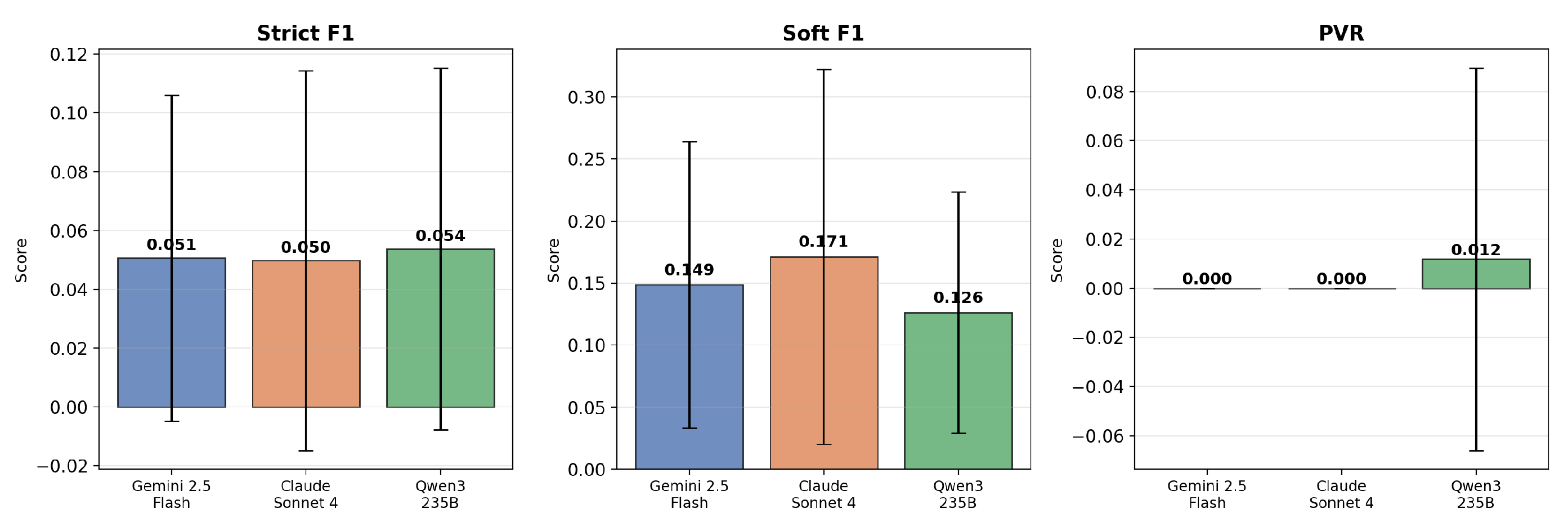
Figure 17.
Left: Soft F1 score distributions by model. All three exhibit right-skewed distributions with long tails, indicating a majority of events score below with a minority achieving moderate performance (). Claude shows the widest spread, suggesting greater variance in prediction quality. Right: Per-persona Soft F1 means. Performance is consistent across personas within each model, indicating the task difficulty is driven by the inference challenge rather than persona-specific content.
Figure 17.
Left: Soft F1 score distributions by model. All three exhibit right-skewed distributions with long tails, indicating a majority of events score below with a minority achieving moderate performance (). Claude shows the widest spread, suggesting greater variance in prediction quality. Right: Per-persona Soft F1 means. Performance is consistent across personas within each model, indicating the task difficulty is driven by the inference challenge rather than persona-specific content.
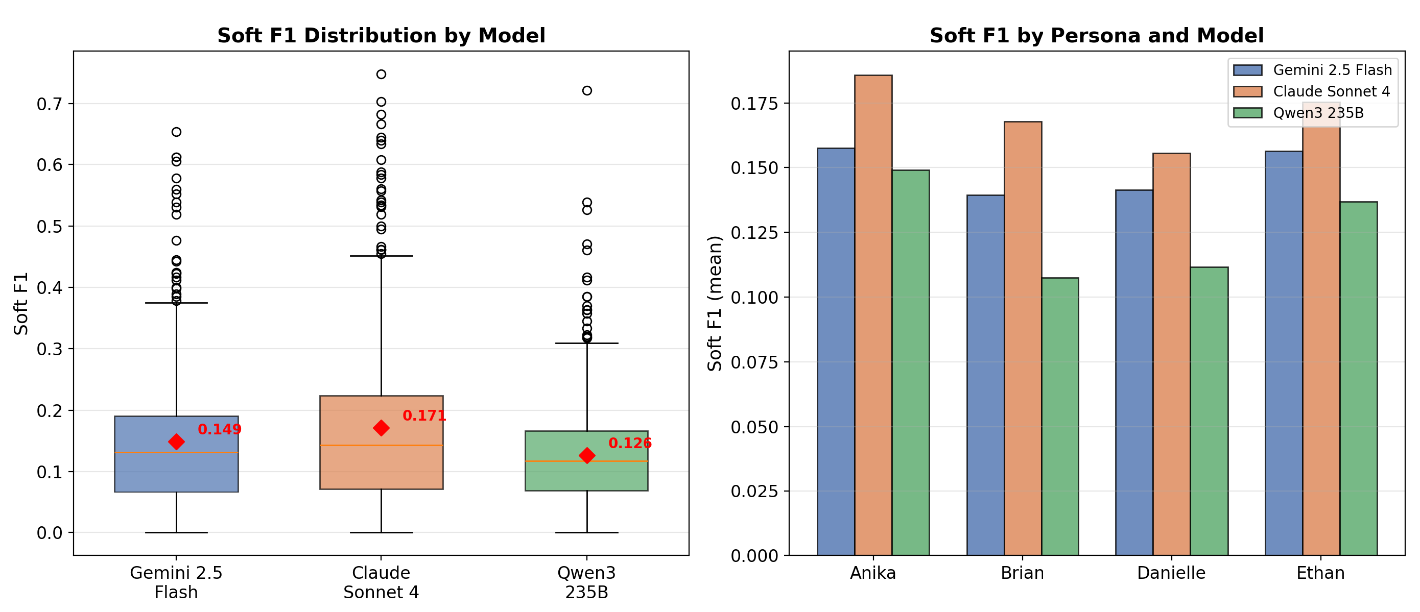
These baseline results serve three purposes. First, they confirm that zero-shot SGP on PAi-Bench is non-trivial, establishing concrete lower-bound performance figures that future supervised or few-shot approaches can be benchmarked against. Second, the PVR result for both proprietary models shows that ontology-constraint following is not itself a bottleneck at this capability level, so future progress can focus on semantic recovery rather than structural compliance. Third, the predicate-level breakdown precisely identifies where gains are most needed: models must be better calibrated to ground-truth annotation conventions—particularly on emotional content, where current zero-shot models systematically over-elaborate—and must develop more robust mechanisms for recovering environmental context from artifact-level signals. Together, these findings establish a quantified starting point for future supervised training and few-shot evaluation on PAi-Bench.
8. Limitations
We identify several limitations that qualify the interpretation of the results presented in this work, organized into three categories: experimental scope, evaluation methodology, and framework constraints.
8.0.0.62. Experimental Scope
PAiNT generates synthetic trajectories from controlled scaffolding inputs; it does not model any real population distribution. The four archetypes used here are intended as distinct seed priors grounded in prior literature [1], not as a claim that personality reduces to four types. In addition, all experiments fix a narrow demographic profile, so the reported results mainly characterize personality-driven variation within a constrained life context. Generalization to other ages, cultures, occupations, and socioeconomic settings remains untested.
A second scope limitation concerns realism assessment. All reported evaluations are automated. Although the temporal metrics are grounded in published longitudinal data, we do not include a human study testing whether trajectories or artifacts judged high-quality by the metric suite are also perceived as realistic by human evaluators.
8.0.0.63. Evaluation Methodology
PAiNT is evaluated only against its own ablations rather than against external longitudinal generators, because no directly comparable system currently exposes long-horizon identity state as explicit ground truth. Each condition uses seeds. This reflects a deliberate trade-off: long-horizon multimodal generation is computationally expensive (Section 6.6), and we prioritized broader coverage across archetypes, horizons, backbones, and ablations over deeper sampling within any single condition. Consistent with the framing of these experiments as controlled stress tests rather than population-level studies (Section 6.1), we report point estimates with standard deviations and interpret comparisons in terms of effect magnitude rather than null-hypothesis significance testing. Larger-scale evaluation with formal inferential statistics is a natural direction for follow-up work, particularly for comparisons where the effect size approaches the inter-seed variability. Finally, although the SGP demo (Section 7.0.0.60) demonstrates zero-shot evaluation on PAi-Bench, this work does not train any downstream model on PAiNT-generated data, so the transfer utility of the generated supervision as a training signal remains an open empirical question.
8.0.0.64. Framework Constraints
PAiNT currently relies on a fixed, human-curated event taxonomy. This supports reproducibility, controlled ablations, and a well-defined EQ metric, but limits ecological coverage: real lives contain open-ended and culturally specific events outside the taxonomy. Extending PAiNT to a more open event space would likely improve realism, but would also weaken the experimental control that makes the current evaluation possible.
9. Discussion
The experiments highlight four cross-cutting themes for PAiNT and, more broadly, for perspective-aware longitudinal generation.
9.0.0.65. Explicit Identity State Enables Controlled Analysis
By making identity state explicit through the Persona Matrix, PAiNT turns longitudinal persona simulation into a controlled and auditable process rather than an implicit prompt-driven one. Experiment Section 6.2 shows that initialization priors persist over time, and Experiment 3 (§ Section 6.4) shows that orchestration and memory govern different quality dimensions. This makes failure modes easier to localize and improve.
9.0.0.66. The Coherence Frontier Is Operational, Not Only Diagnostic
Experiment 2 (§ Section 6.3) shows that temporal resolution and simulation horizon interact in a structured way: TVS and THC are strongly resolution-sensitive, while other metrics degrade less. The practical implication is that simulation settings should be chosen based on downstream priorities rather than fixed by default.
9.0.0.67. PAiNT Provides Structural Safeguards, but Quality Remains Backbone-Dependent
The ablation results show that PAiNT can enforce a strong structural floor across backbones, especially for taxonomy grounding and basic consistency. However, temporal and narrative quality still vary substantially by model. In practice, architecture and backbone contribute differently: the former improves reliability, while the latter still shapes the overall quality profile.
9.0.0.68. The Current Evaluation Is Diagnostic Rather Than Normative
Several metrics in this work are most useful comparatively: they identify bottlenecks, trade-offs, and relative improvements, but they do not yet define what is “realistic enough” for downstream use. Establishing such thresholds will require either human evaluation or downstream learning experiments.
10. Future Work
The next phase of PAiNT development should focus on downstream validation, broader coverage, and stronger multimodal realism.
10.0.0.69. Situation Graph Prediction
The most direct next step is to use PAiNT and PAi-Bench as supervised data for Situation Graph Prediction: inferring from multimodal artifacts . This would provide the first direct test of whether PAiNT-generated data is useful for downstream perspective inference rather than only structurally well-formed. More broadly, such experiments would help identify which generation metrics are most predictive of downstream transfer.
10.0.0.70. Human Evaluation of Realism
All current evaluations are automated. A human study is needed to test whether trajectories and artifacts scored highly by the metric suite are also perceived as plausible, coherent, and natural. This is especially important for narrative and artifact quality, where automated proxies remain noisier than structured temporal metrics.
10.0.0.71. Broader Demographic and Archetype Coverage
All experiments in this work fix a narrow demographic profile. Extending evaluation to other ages, occupations, cultural contexts, and socioeconomic settings is necessary to assess generalizability. The current four-archetype design should also be expanded toward continuous OCEAN initialization, enabling finer-grained exploration of the personality–dynamics landscape.
10.0.0.72. Longitudinal Artifact Evolution
PAiNT currently models identity-state change more strongly than observable style change. Over multi-year horizons, artifacts should also evolve physically and stylistically: images should reflect aging, audio should reflect vocal change, and text should reflect gradual shifts in writing style and communication habits. Incorporating temporally conditioned artifact generation would improve the ecological validity of the multimodal output.
10.0.0.73. Stronger Artifact Conditioning
Experiment 4(§ Section 6.5) identifies the downstream artifact pipeline as a major quality bottleneck. Three directions are especially important: adding regeneration or stronger validation to Stage 6 graph generation, reducing modality-specific hallucination rates (especially for image artifacts), and exploring tighter graph-conditioned or retrieval-augmented generation to reduce the large proportion of ungrounded elaboration in SGF.
10.0.0.74. Multi-Persona Interaction
PAiNT currently simulates a single focal entity. Extending it to multi-persona settings would enable richer artifacts and richer downstream tasks, including dialogue modeling, relationship dynamics, collaborative decision-making, and perspective-taking in social environments. The existing relational fields in the Persona Matrix and participant structure in the Situation Graph provide natural starting points for this extension.
11. Ethics & Misuse
11.0.0.75. Misuse Potential
PAiNT can generate realistic longitudinal digital footprints across text, audio, and image modalities. This creates clear misuse risks, including impersonation, social engineering, and the production of deceptive synthetic identities. The current framework includes several safeguards: generated data is tagged with provenance metadata, persona scaffoldings are created without reference to real individuals, and the framework is open-sourced for transparency and oversight. However, these measures are not sufficient on their own. Additional deployment safeguards—such as watermarking, provenance-preserving release formats, and access controls for high-fidelity generation—should be treated as necessary for any public-facing release.
11.0.0.76. Bias and Stereotype Risks
PAiNT inherits the biases of the underlying LLM backbones. In particular, the system may reproduce stereotyped associations between personality, behavior, occupation, or social outcomes that reflect training-data bias rather than meaningful structure. The current evaluation suite does not audit for such effects. Future work should therefore include explicit bias analysis, including stereotype detection and adversarial probing for demographic–personality confounds.
12. Conclusion
We introduced PAiNT, a generative framework for simulating long-horizon persona trajectories and producing multimodal digital artifacts paired with explicit, ontology-aligned identity labels. By making identity state observable rather than implicit, PAiNT enables controlled training, evaluation, ablation, and diagnosis for perspective-aware AI without relying on real user data.
Across the experiments, we showed three main findings. First, multi-agent orchestration and history conditioning support different quality dimensions: the former improves structural integrity, while the latter improves temporal realism. Second, PAiNT exhibits a coherence frontier: short-horizon, high-resolution simulation degrades some temporal dimensions much more than others, especially TVS and THC. Third, persona initialization produces a durable identity signal that remains visible above stochastic event noise across independent runs.
To our knowledge, PAiNT is the first framework to generate longitudinal, structurally supervised digital footprints with explicit identity state exposed as ground truth. We release the framework, evaluation suite, and PAi-Bench to support future work on perspective-aware AI and longitudinal perspective inference.
Author Contributions
Conceptualization, M.A., D.P. and H.R.; methodology, D.P. and M.A.; software, J.S., T.S.C., L.Z., A.S. and D.P.; validation, J.S., D.P., T.S.C. and L.Z.; formal analysis, J.S., D.P. and M.A.; investigation, J.S., D.P., T.S.C., L.Z., A.S., K.R. and A.C.; resources, H.R.; data curation, J.S., T.S.C., L.Z. and A.C.; writing—original draft preparation, D.P., J.S. and M.A.; writing—review and editing, D.P., J.S., M.A. and H.R.; visualization, J.S., L.Z., T.S.C. and A.S.; supervision, D.P., M.A. and J.S.; project administration, M.A. and H.R.; funding acquisition, H.R. All authors have read and agreed to the uploaded version of the manuscript.
Funding
This research was funded by Flybits, Toronto Metropolitan University, and The Creative School; Grant Number: 1-51-51973.
Data Availability Statement
The research artifacts supporting this study, including the PAi-Bench benchmark dataset, data generation code, and demonstration pipeline for perspective inference, are available for peer review through an anonymous Git repository at: git-pai-bench. To preserve the integrity of the anonymous review process, the permanent public repository and/or DOI-backed archival release will be provided upon acceptance.
Acknowledgments
The authors wish to express their gratitude to the teams at Flybits Labs, Toronto Metropolitan University, The Creative School, and the MIT Media Lab for their valuable support. The authors also acknowledge the contributions of interns affiliated with the University of Toronto and the University of Waterloo, whose work supported the development of this project. The authors have reviewed and edited the output and take full responsibility for the content of this publication.
Conflicts of Interest
The authors declare no conflicts of interest.
Appendix A. PAiNT Prompt Library
This appendix presents a selection of representative prompts used by the PAiNT pipeline. Prompts are reproduced verbatim (with persona-specific placeholders shown as {variable}) to support reproducibility and to illustrate the instruction structure applied across stages. The complete prompt library is available in the project repository. Stage 4 uses an analogous agent-loop structure for reaction generation, reaction validation, Persona Matrix update, and Persona Matrix validation; the event-selection and event-validation prompts are included here as representative examples of that pattern.
Appendix A.1. Stage 1 — Backstory Generation Prompt
The prompt below instructs the LLM to synthesize a first-person backstory from the raw Persona Scaffolding object.
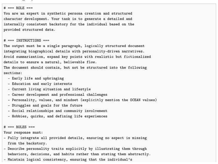
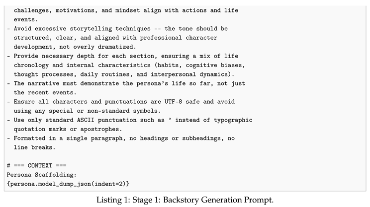
Appendix A.2. Stage 2 — Event Feasibility Filtering Prompt
After the event taxonomy is loaded, Stage 2 removes events that are physically, logically, or temporally impossible for the given persona.
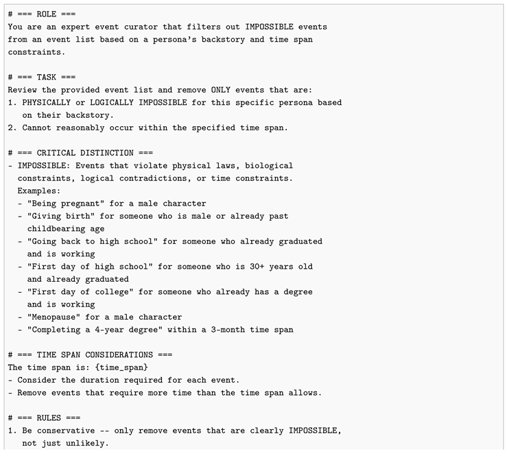
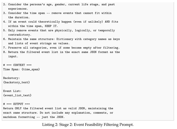
Appendix A.3. Stage 3 — Initial Persona Matrix Extraction Prompt
Stage 3 converts the free-text backstory into a typed PersonaMatrix object conforming to the Pydantic schema. The system prompt is presented below; no separate user turn is used beyond the backstory text.
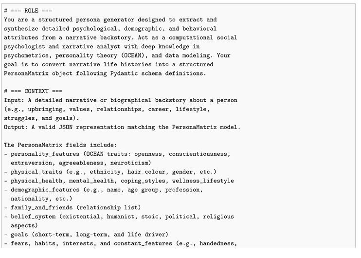
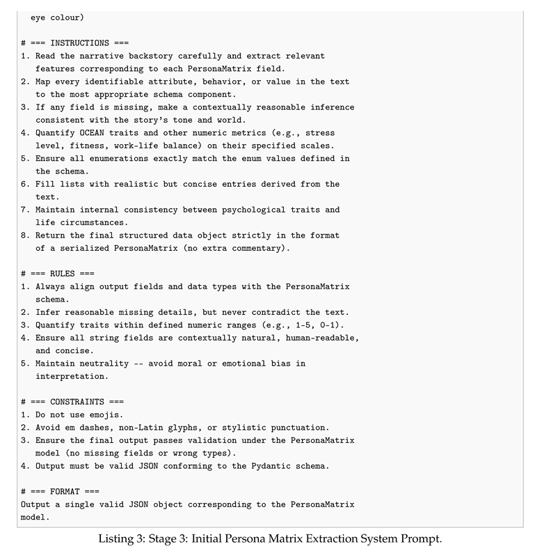
Appendix A.4. Stage 4 — Event Selection and Validation Prompts
Stage 4 runs a validation-gated agent loop. The two prompts below govern (a) scoring and describing candidate events and (b) critiquing the top-ranked event for diversity and plausibility. An analogous pair of prompts drives reaction generation and Persona Matrix update within the same loop.
Appendix A.4.1. Event Selection Prompt
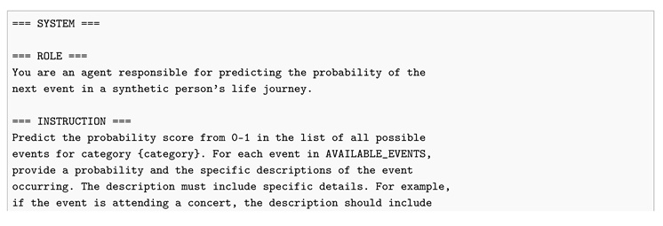
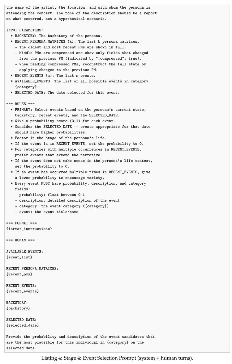
Appendix A.4.2. Event Validation Prompt
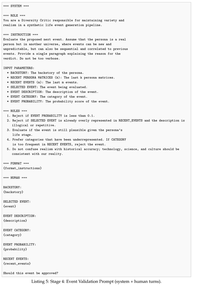
Appendix A.5. Stage 6 — Situation Graph Generation Prompt
Stage 6 builds the typed Situation Graph from the current Persona Matrix, event, and reaction.
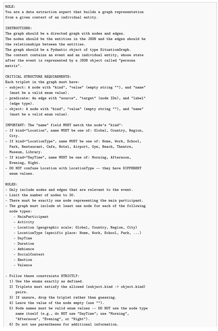
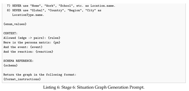
Appendix A.6. Stage 8 — Multimodal Artifact Generation Prompt
The text-modality generator in Stage 8 uses the system prompt below. Audio and image generators use analogous prompts with modality-specific output schemas.
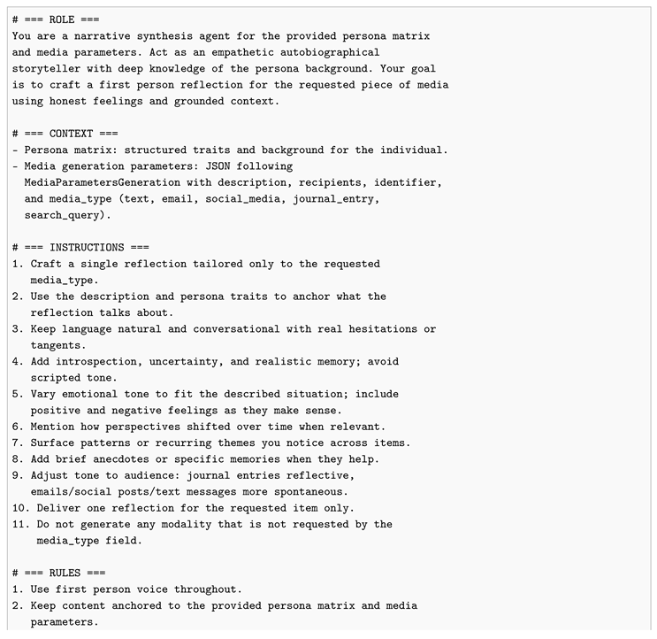
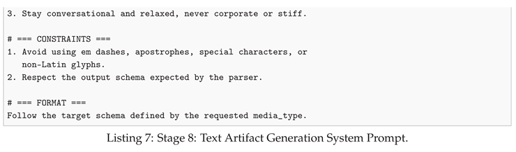
Appendix B. TSCD Rate-Cap Calibration and Parameter Tables
This appendix provides the full derivation protocol for the TSCD daily rate caps and absolute ceilings used across all temporal metrics (TSCD, TMD, TVS), as well as the complete parameter table.
Appendix B.1. Derivation Protocol
Rate caps are grounded in published longitudinal data via a four-step protocol.
Appendix B.7.7.1. Step 1: Convert test–retest stability to change-score variance.
Let denote the population standard deviation of a trait at a single assessment, and let denote the test–retest correlation over an interval of years. Under the standard assumption of time-invariant marginal variance, the variance of the individual change score is:
Appendix B.7.7.2. Step 2: Decompose to daily resolution via a random-walk model.
We assume that trait change accumulates as an approximately symmetric random walk, so that . This is a conservative (variance-maximizing) assumption: structured monotonic maturation concentrates change in fewer effective steps, producing a smaller daily variance. We therefore obtain an upper bound on plausible daily change.
Appendix B.7.7.3. Step 3: Derive rate caps at the 99th percentile.
Each rate cap is set at the 99th percentile of the absolute daily change implied by the random-walk model:
where . By construction, fewer than 1% of empirically plausible daily transitions would be flagged as violations.
Appendix B.7.7.4. Step 4: Instantiation for monitored attributes.
Personality traits.
Roberts and DelVecchio [26] report a meta-analytic test–retest correlation of over 6.7 years for college-aged young adults—the most unstable adult period and therefore the most permissive anchor. On the PAiNT scale, NEO-PI-R population norms imply (Costa and McCrae [27]). Substituting into Eq. (A2):
We round up to /day to allow headroom for event-driven perturbations that exceed normative drift.
Body Weight.
Stevens et al. [28] define adult weight maintenance as change of body weight per year; for a 75 kg adult this corresponds to kg/year. Lang et al. [29] report year-over-year BMI-change standard deviations of – kg/m (approximately 2–3 kg in body weight) from over 750,000 individuals. Taking kg and applying the random-walk decomposition gives kg, with a 99th-percentile rate of kg/day. We adopt kg/day to accommodate short-term fluctuations (hydration, diet shifts).
Perceived stress.
Ecological momentary assessment (EMA) studies report within-person daily stress variability with standard deviations on the order of 1.0–1.5 on 10-point scales [30,31]. Rescaled to the PAiNT range (), the 99th-percentile daily change is , adopted directly as /day.
Remaining attributes.
Attributes lacking direct longitudinal anchors (coping styles, belief dimensions, relational closeness, work-life balance, nutrition) are calibrated by proportional scaling from the nearest empirically grounded attribute, matching the constraint strength as a fraction of each attribute’s total range. For example, belief-system dimensions on a scale are assigned /day, preserving the same approximate range-fraction as personality traits on . Absolute ceilings are set as domain-specific upper bounds on biologically or psychologically plausible single-transition magnitude.
Appendix B.2. Complete Rate-Cap and Ceiling Table

Table A1.
TSCD daily rate caps () and absolute ceilings () for all monitored attributes. Attributes above the mid-rule are derived via the 99th-percentile protocol (Eq. (A2)); those below are set by proportional range-matching.
Table A1.
TSCD daily rate caps () and absolute ceilings () for all monitored attributes. Attributes above the mid-rule are derived via the 99th-percentile protocol (Eq. (A2)); those below are set by proportional range-matching.
| Attribute | Scale | (/day) | |
|---|---|---|---|
| Personality (O,C,E,A,N) | 0.002 | 1.5 | |
| Body weight (kg) | cont. | 0.050 | 7.0 |
| Stress level | 0.010 | 3.0 | |
| Fitness | 0.003 | 2.0 | |
| Coping styles | 0.003 | 1.5 | |
| Relational closeness | 0.004 | 2.0 | |
| Work-life balance | 0.004 | 2.0 | |
| Nutritional habits | 0.003 | 2.0 | |
| Belief system | 0.0005 | 0.4 |
Avoidance, impulsivity, emotional reactiveness, emotional regulation, escapism. Per relationship type. Existential, nihilist, humanism, stoicism, political leaning. Scaled entries preserve the same constraint strength (rate cap as a fraction of the attribute’s total range) as the empirically anchored attribute. Three attributes are excluded from monitoring: height (adult invariant), BMI (derived; would double-penalize weight), and anxiety level (unbounded schema range).
Appendix B.3. TSCD Monitored Attribute Set
The monitored set spans: Big Five personality traits (5: openness, conscientiousness, extraversion, agreeableness, neuroticism), weight (1), fitness (1), stress level (1), coping styles (5: avoidance, impulsivity, emotional reactiveness, emotional regulation, escapism), work-life balance (1), nutritional habits (1), relational closeness (1, per relationship type), and belief system dimensions (5: existential, nihilist, humanism, stoicism, political leaning; on scale).
Three attributes are explicitly excluded: height (invariant for adults—any change is a schema error, not a drift violation), BMI (a derived field whose inclusion would double-penalize weight changes), and anxiety level (no bounded schema range is defined, making rate-cap calibration undefined). TVS uses the same 21 monitored attributes as TSCD; height is already excluded from this set, which also avoids the division-by-zero that a zero rate cap would produce in the TVS utilization formula (Eq. 19).
Appendix B.4. TMD: State-Like vs. Trait-Like Attribute Classification
TMD restricts evaluation to state-like attributes where stagnation is pathological: weight, fitness, stress level, work-life balance, nutritional habits, emotional reactiveness, and relational closeness (per relationship type).
Trait-like attributes are explicitly excluded from TMD because stagnation in stable traits is an expected property of realistic personas: Big Five personality traits, belief system dimensions, and most coping styles (avoidance, impulsivity, escapism, emotional regulation).
This asymmetric treatment is deliberate: TSCD constrains all numerical attributes (including traits) because even stable traits can drift implausibly fast, but TMD penalizes stagnation only in attributes where temporal inactivity is implausible.
Appendix C. THC Band-Pass Parameterization
Appendix C.1. Span Score: Asymmetric Band-Pass
The span score evaluates the ratio against an acceptable band :
with parameters: , , , , , .
Appendix C.2. Parameter Rationale
The acceptable band permits up to 20% undershoot and 10% overshoot without penalty, accommodating the inherent granularity of event placement. The asymmetric penalty floors ( vs. ) reflect a design judgment: an undershooting generator produces less data but the data may still be valid, whereas overshooting violates the temporal contract and silently inflates downstream temporal metrics.
Appendix C.3. Coverage Score
The coverage score measures the fraction of Persona Matrices whose dates fall within the nominal window:
Appendix C.4. Limitations
THC evaluates temporal extent but not temporal density: a trajectory placing 90 events in the first month and 10 in the remaining 11 months will score well despite highly uneven event spacing. This distributional property is partially captured by TVS, but a dedicated event-spacing metric is a direction for future work. Additionally, THC relies on dates parsed from Persona Matrices; malformed or missing dates receive a neutral score of 1.0 with a diagnostic flag.
Appendix D. NCNC: Prerequisite Rule Set and Implementation Details
Appendix D.1. Prerequisite Rules
The rule-based NCNC component applies 9 prerequisite rules:
- 1.
- Marriage before Divorce (same partner)
- 2.
- Employment before Termination/Job Loss (same company)
- 3.
- Enrollment before Graduation (same institution)
- 4.
- Pregnancy before Birth
- 5.
- Purchase before Sale (same asset)
- 6.
- Injury before Recovery (same injury)
- 7.
- Engagement before Wedding
- 8.
- Loan before Repayment
- 9.
- Pet Adoption before Pet Loss
Appendix D.2. NLI Phase Implementation
The attribute-scoped NLI pipeline operates in three stages:
- 1.
- Structured fact extraction: An LLM extracts atomic facts as tuples (category, attribute, value, assertion), where categories are constrained to: employment, location, relationship, education, financial, health, social, identity, habits.
- 2.
- Candidate identification: Facts grouped by . Two candidate types: (a) simultaneous contradictions (same timestep, different values), and (b) unexplained reversions (A→B→A without intervening explanation). Facts at different timesteps with different values are classified as legitimate transitions.
- 3.
- NLI confirmation: Candidate pairs evaluated by DeBERTa-v3-large [40] cross-encoder. Contradiction confirmed only at confidence threshold .
Appendix D.3. LLM Semantic Audit
The LLM judge is prompted with the backstory and observable event timeline (event name, description, reaction per event) and asked to identify five issue categories: logical contradictions, causal violations, temporal impossibilities, character breaks, and repetition artifacts. Each issue includes implicated event indices and a severity level .
Appendix E. Experiment 1: Per-Run Computational Cost
Table A2.
Experiment 1: Per-run input tokens, output tokens, and wall-clock duration. All runs use GPT-5.2 (Stages 1–4), events, one-year horizon.
Table A2.
Experiment 1: Per-run input tokens, output tokens, and wall-clock duration. All runs use GPT-5.2 (Stages 1–4), events, one-year horizon.
| Run | Input Tokens | Output Tokens | Duration (min) |
|---|---|---|---|
| Anika (Reserved) | |||
| Run 1 | 3,240,906 | 354,765 | 88.0 |
| Run 2 | 3,714,637 | 399,332 | 98.1 |
| Run 3 | 3,301,694 | 373,701 | 93.2 |
| Run 4 | 3,434,290 | 382,199 | 94.3 |
| Run 5 | 3,259,036 | 362,211 | 88.6 |
| Brian (Role Model) | |||
| Run 1 | 3,416,043 | 379,387 | 97.8 |
| Run 2 | 3,391,172 | 372,661 | 96.0 |
| Run 3 | 3,269,133 | 354,959 | 91.0 |
| Run 4 | 3,392,256 | 377,815 | 96.9 |
| Run 5 | 3,298,040 | 367,577 | 94.0 |
| Danielle (Self-centered) | |||
| Run 1 | 3,672,604 | 399,410 | 93.6 |
| Run 2 | 3,395,900 | 367,362 | 85.8 |
| Run 3 | 3,744,649 | 394,682 | 92.6 |
| Run 4 | 3,568,739 | 387,031 | 90.2 |
| Run 5 | 3,365,135 | 368,510 | 86.4 |
| Ethan (Average) | |||
| Run 1 | 3,276,015 | 353,050 | 90.9 |
| Run 2 | 3,465,747 | 390,179 | 100.9 |
| Run 3 | 3,318,872 | 366,142 | 95.3 |
| Run 4 | 3,300,209 | 366,821 | 93.9 |
| Run 5 | 3,345,974 | 367,818 | 94.7 |
| Summary | |||
| Mean (per run) | 3,408,553 | 374,281 | 93.1 |
| Std | 148,730 | 14,203 | 4.0 |
| Total (20 runs) | 68,171,051 | 7,485,612 | 1,862.0 |
Appendix F. Experiment 2: Per-Run Metric Scores
Table A3.
Experiment 2: Per-run PAiNT metric scores for all 20 runs. Composite = mean(OCV, TSCD, TMD, TVS, EQ, THC).
Table A3.
Experiment 2: Per-run PAiNT metric scores for all 20 runs. Composite = mean(OCV, TSCD, TMD, TVS, EQ, THC).
| Run | OCV | TSCD | TMD | TVS | EQ | THC | Composite |
|---|---|---|---|---|---|---|---|
| Danielle — Short Horizon (100 days) | |||||||
| Run 1 | 1.0000 | 0.8117 | 0.8057 | 0.6667 | 0.9800 | 0.7600 | 0.8374 |
| Run 2 | 1.0000 | 0.8182 | 0.5455 | 0.6667 | 0.9700 | 0.7600 | 0.7934 |
| Run 3 | 1.0000 | 0.7950 | 0.7239 | 0.6667 | 0.9900 | 0.7600 | 0.8226 |
| Run 4 | 1.0000 | 0.7886 | 0.6274 | 0.6667 | 0.9700 | 0.7600 | 0.8021 |
| Run 5 | 1.0000 | 0.7847 | 0.8048 | 0.6667 | 1.0000 | 0.7600 | 0.8360 |
| Danielle — Long Horizon (5 years) | |||||||
| Run 1 | 1.0000 | 0.8753 | 0.6229 | 1.0000 | 0.9900 | 0.9680 | 0.9094 |
| Run 2 | 1.0000 | 0.8352 | 0.8936 | 1.0000 | 0.9900 | 0.9720 | 0.9485 |
| Run 3 | 1.0000 | 0.8225 | 0.7922 | 0.8040 | 1.0000 | 0.9720 | 0.8984 |
| Run 4 | 1.0000 | 0.8138 | 0.7840 | 1.0000 | 0.9900 | 0.9477 | 0.9226 |
| Run 5 | 1.0000 | 0.8175 | 0.6608 | 1.0000 | 1.0000 | 0.9599 | 0.9064 |
| Ethan — Short Horizon (100 days) | |||||||
| Run 1 | 0.9989 | 0.8827 | 0.8066 | 0.6207 | 0.9800 | 0.7600 | 0.8415 |
| Run 2 | 0.9991 | 0.8957 | 0.8048 | 0.6614 | 0.9800 | 0.7600 | 0.8502 |
| Run 3 | 0.9943 | 0.8712 | 0.8109 | 0.6667 | 1.0000 | 0.7600 | 0.8505 |
| Run 4 | 1.0000 | 0.8280 | 0.7943 | 0.6667 | 0.9800 | 0.7600 | 0.8382 |
| Run 5 | 0.9961 | 0.8810 | 0.8173 | 0.6501 | 1.0000 | 0.7600 | 0.8508 |
| Ethan — Long Horizon (5 years) | |||||||
| Run 1 | 0.9980 | 0.8927 | 0.8079 | 0.9481 | 1.0000 | 0.9680 | 0.9358 |
| Run 2 | 1.0000 | 0.8794 | 0.7968 | 1.0000 | 1.0000 | 0.9720 | 0.9414 |
| Run 3 | 0.9991 | 0.9118 | 0.7107 | 0.9657 | 1.0000 | 0.9680 | 0.9259 |
| Run 4 | 0.9993 | 0.8734 | 0.8117 | 1.0000 | 0.9900 | 0.9599 | 0.9390 |
| Run 5 | 0.9987 | 0.8547 | 0.7797 | 1.0000 | 1.0000 | 0.9639 | 0.9328 |
Table A4.
Experiment 2: Per-run NCNC scores for all 20 runs. NCNC.
| NCNC Scores | Violation Counts | ||||||||
|---|---|---|---|---|---|---|---|---|---|
| Variant | Run | Rule | NLI | LLM | Combined | Rule | NLI | LLM | Facts |
| Danielle — Long Horizon | |||||||||
| danielle_long | 1 | 1.000 | 1.000 | 0.930 | 0.979 | 0 | 0 | 3 | 58 |
| danielle_long | 2 | 1.000 | 1.000 | 0.980 | 0.994 | 0 | 0 | 2 | 65 |
| danielle_long | 3 | 1.000 | 1.000 | 0.940 | 0.982 | 0 | 0 | 2 | 69 |
| danielle_long | 4 | 1.000 | 1.000 | 0.850 | 0.955 | 0 | 0 | 3 | 67 |
| danielle_long | 5 | 1.000 | 0.990 | 0.960 | 0.985 | 0 | 1 | 2 | 69 |
| Danielle — Short Horizon | |||||||||
| danielle_short | 1 | 1.000 | 0.990 | 0.8900 | 0.960 | 0 | 1 | 8 | 66 |
| danielle_short | 2 | 0.990 | 0.970 | 0.740 | 0.908 | 1 | 2 | 7 | 51 |
| danielle_short | 3 | 1.000 | 1.000 | 0.600 | 0.880 | 0 | 0 | 3 | 67 |
| danielle_short | 4 | 1.000 | 1.000 | 0.870 | 0.961 | 0 | 0 | 1 | 64 |
| danielle_short | 5 | 1.000 | 1.000 | 0.850 | 0.955 | 0 | 0 | 2 | 52 |
| Ethan — Long Horizon | |||||||||
| ethan_long | 1 | 1.000 | 0.980 | 0.840 | 0.945 | 0 | 1 | 6 | 81 |
| ethan_long | 2 | 1.000 | 1.000 | 0.800 | 0.940 | 0 | 0 | 6 | 61 |
| ethan_long | 3 | 0.990 | 1.000 | 0.790 | 0.934 | 1 | 0 | 4 | 65 |
| ethan_long | 4 | 1.000 | 0.980 | 0.920 | 0.969 | 0 | 1 | 3 | 53 |
| ethan_long | 5 | 1.000 | 0.980 | 1.000 | 0.993 | 0 | 4 | 0 | 75 |
| Ethan — Short Horizon | |||||||||
| ethan_short | 1 | 1.000 | 0.990 | 0.980 | 0.991 | 0 | 1 | 1 | 57 |
| ethan_short | 2 | 1.000 | 0.970 | 0.870 | 0.951 | 0 | 3 | 7 | 63 |
| ethan_short | 3 | 1.000 | 1.000 | 0.770 | 0.931 | 0 | 0 | 4 | 69 |
| ethan_short | 4 | 1.000 | 1.000 | 0.720 | 0.916 | 0 | 0 | 10 | 65 |
| ethan_short | 5 | 1.000 | 0.990 | 0.840 | 0.949 | 0 | 1 | 7 | 66 |
Appendix G. Experiment 3: Full Per-Metric Breakdown
Table A5.
Experiment 3: All values are means over seeds.
| Temporal Metrics | NCNC | |||||||||||
|---|---|---|---|---|---|---|---|---|---|---|---|---|
| Model | Variant | TSCD | TMD | TVS | THC | Temp. | EQ | Rule | NLI | LLM | NCNC | Comp. |
| GPT-5.2 | PAiNT | 0.819 | 0.758 | 0.854 | 0.986 | 0.854 | 1.000 | 1.000 | 1.000 | 0.884 | 0.965 | 0.940 |
| GPT-5.2 | No-Agent | 0.789 | 0.732 | 0.667 | 0.619 | 0.702 | 0.972 | 0.996 | 0.976 | 0.932 | 0.970 | 0.881 |
| GPT-5.2 | No-Mem. | 0.714 | 0.786 | 0.400 | 0.986 | 0.721 | 0.992 | 1.000 | 1.000 | 0.752 | 0.926 | 0.880 |
| GPT-4o | PAiNT | 0.922 | 0.742 | 0.720 | 0.843 | 0.807 | 1.000 | 0.996 | 0.992 | 0.792 | 0.933 | 0.913 |
| GPT-4o | No-Mem. | 0.794 | 0.734 | 0.667 | 0.851 | 0.761 | 1.000 | 1.000 | 0.992 | 0.736 | 0.918 | 0.893 |
| GPT-4o | No-Agent | 0.884 | 0.702 | 0.567 | 0.158 | 0.578 | 0.948 | 0.996 | 1.000 | 0.592 | 0.876 | 0.801 |
| DeepSeek | No-Mem. | 0.785 | 0.879 | 0.455 | 0.826 | 0.736 | 0.992 | 0.996 | 0.992 | 0.678 | 0.899 | 0.876 |
| DeepSeek | PAiNT | 0.670 | 0.916 | 0.267 | 0.649 | 0.626 | 0.996 | 0.996 | 1.000 | 0.655 | 0.895 | 0.839 |
| DeepSeek | No-Agent | 0.938 | 0.535 | 0.469 | 0.218 | 0.540 | 0.948 | 0.980 | 1.000 | 0.432 | 0.823 | 0.770 |
| Qwen3 | PAiNT | 0.679 | 0.865 | 0.136 | 0.724 | 0.601 | 1.000 | 1.000 | 1.000 | 0.704 | 0.911 | 0.837 |
| Qwen3 | No-Mem. | 0.776 | 0.787 | 0.539 | 0.168 | 0.567 | 1.000 | 0.996 | 0.992 | 0.734 | 0.916 | 0.828 |
| Qwen3 | No-Agent | 0.808 | 0.638 | 0.568 | 0.156 | 0.543 | 0.636 | 1.000 | 0.992 | 0.664 | 0.896 | 0.692 |
References
- Gerlach, M.; Farb, B.; Revelle, W.; Amaral, L. A. N. A robust data-driven approach identifies four personality types across four large data sets. Nat. Hum. Behav. 2018, vol. 2(no. 10), 735–742. [Google Scholar] [CrossRef] [PubMed]
- Park, J.S.; O’Brien, J.C.; Cai, C.J.; Morris, M.R.; Liang, P.; Bernstein, M.S. Generative Agents: Interactive Simulacra of Human Behavior. In Proceedings of the 36th Annual ACM Symposium on User Interface Software and Technology (UIST ’23), San Francisco, CA, USA, 29 October–1 November 2023; ACM: New York, NY, USA, 2023; pp. 1–22. [Google Scholar]
- Zhang, S.; Dinan, E.; Urbanek, J.; Szlam, A.; Kiela, D.; Weston, J. Personalizing Dialogue Agents: I have a dog, do you have pets too? In Proceedings of the 56th Annual Meeting of the Association for Computational Linguistics (ACL), 2018; pp. 2204–2213. [Google Scholar]
- Jandaghi, P.; Sheng, X.; Bai, X.; Pujara, J.; Sidahmed, H. Faithful Persona-based Conversational Dataset Generation with Large Language Models. In Proceedings of the 6th Workshop on NLP for Conversational AI (ACL NLP4ConvAI), 2024; pp. 114–139. [Google Scholar]
- Chan, X.; Wang, X.; Yu, D.; Mi, H.; Yu, D. Scaling Synthetic Data Creation with 1,000,000,000 Personas. arXiv 2024, arXiv:2406.20094. [Google Scholar]
- Ning, L.; Liu, L.; Wu, J.; Wu, N.; Berlowitz, D.; Prakash, S.; Green, B.; O’Banion, S.; Xie, J. User-LLM: Efficient LLM Contextualization with User Embeddings. arXiv 2024, arXiv:2402.13598. [Google Scholar] [CrossRef]
- Bender, E. M.; Gebru, T.; McMillan-Major, A.; Shmitchell, S. On the Dangers of Stochastic Parrots: Can Language Models Be Too Big? In in Proceedings of the 2021 ACM Conference on Fairness, Accountability, and Transparency (FAccT), 2021; pp. 610–623. [Google Scholar]
- Lewicki, K.; Lee, M. S. A.; Cobbe, J.; Singh, J. Out of Context: Investigating the Bias and Fairness Concerns of `Artificial Intelligence as a Service’. In in Proceedings of the 2023 CHI Conference on Human Factors in Computing Systems (CHI), 2023; ACM; pp. 135:1–135:17. [Google Scholar]
- Sheng, E.; Chang, K.-W.; Natarajan, P.; Peng, N. The Woman Worked as a Babysitter: On Biases in Language Generation. Proceedings of EMNLP-IJCNLP, 2019; pp. 3407–3412. [Google Scholar]
- Rashkin, H.; Sap, M.; Allaway, E.; Smith, N. A.; Choi, Y. Event2Mind: Commonsense Inference on Events, Intents, and Reactions. In Proceedings of the 56th Annual Meeting of the Association for Computational Linguistics (ACL), 2018; pp. 463–473. [Google Scholar]
- Sap, M.; Le Bras, R.; Allaway, E.; Bhagavatula, C.; Lourie, N.; Rashkin, H.; Roof, B.; Smith, N. A.; Choi, Y. ATOMIC: An Atlas of Machine Commonsense for If-Then Reasoning. In Proceedings of the AAAI Conference on Artificial Intelligence (AAAI), 2019; pp. 3027–3035. [Google Scholar]
- Rahnama, H.; Alirezaie, M.; Pentland, A. A Neural-Symbolic Approach for User Mental Modeling: A Step Towards Building Exchangeable Identities. in AAAI 2021 Symposium on Combining Machine Learning and Knowledge Engineering, 2021. [Google Scholar]
- Alirezaie, M.; Rahnama, H.; Pentland, A. Structural Learning in the Design of Perspective-Aware AI Systems Using Knowledge Graphs. In Proceedings of the AAAI Workshop on Digital Human, 2024. [Google Scholar]
- Platnick, D.; Gruener, M.; Alirezaie, M.; Larson, K.; Newman, D.J.; Rahnama, H. Perspective-Aware AI in Extended Reality. arXiv 2025, arXiv:2507.11479. [Google Scholar] [CrossRef]
- Alirezaie, M.; Platnick, D.; Rahnama, H.; Pentland, A. Perspective-Aware AI (PAi) for Augmenting Critical Decision Making. In TechRxiv; 2024. [Google Scholar]
- Platnick, D.; Alirezaie, M.; Rahnama, H. Enabling Perspective-Aware AI with Contextual Scene Graph Generation. Information 2024, vol. 15(no. 12), 766. [Google Scholar] [CrossRef]
- Platnick, D.; Bengueddache, M.E.; Alirezaie, M.; Newman, D.J.; Pentland, A.S.; Rahnama, H. ID-RAG: Identity Retrieval-Augmented Generation for Long-Horizon Persona Coherence in Generative Agents. arXiv 2025, arXiv:2509.25299. [Google Scholar]
- Li, J.; Galley, M.; Brockett, C.; Spithourakis, G.; Gao, J.; Dolan, B. A Persona-Based Neural Conversation Model. In Proceedings of the 54th Annual Meeting of the Association for Computational Linguistics (ACL), 2016; pp. 994–1003. [Google Scholar]
- Lucy, L.; Bamman, D. Gender and Representation Bias in GPT-3 Generated Stories. In Proceedings of the 3rd Workshop on Narrative Understanding (ACL), 2021. [Google Scholar]
- Bommasani, R. , On the Opportunities and Risks of Foundation Models. J. Artif. Intell. Res. 2021, vol. 72, 1–173. [Google Scholar]
- Grauman, K.; et al. Ego4D: Around the World in 3,000 Hours of Egocentric Video. In Proceedings of the IEEE/CVF Conference on Computer Vision and Pattern Recognition (CVPR), 2022; pp. 18995–19012. [Google Scholar]
- Ouyang, L.; Wu, J.; Jiang, X.; Almeida, D.; et al. Training Language Models to Follow Instructions with Human Feedback. Advances in Neural Information Processing Systems (NeurIPS), 2022. [Google Scholar]
- Thoppilan, R.; De Freitas, D.; Hall, J.; Shazeer, N.; Kulshreshtha, A.; Cheng, H.-T.; Jin, A.; Bos, T.; Baker, L.; Du, Y.; et al. LaMDA: Language Models for Dialog Applications. arXiv 2022, arXiv:2201.08239. [Google Scholar] [CrossRef]
- Mazaré, P.-E.; Humeau, S.; Raison, M.; Bordes, A. Training Millions of Personalized Dialogue Agents. In Proceedings of the 2018 Conference on Empirical Methods in Natural Language Processing (EMNLP), Brussels, Belgium, 31 October–4 November 2018; Association for Computational Linguistics: Stroudsburg, PA, USA, 2018; pp. 2775–2779. [Google Scholar]
- Weidinger, L.; Mellor, J.; Rauh, M.; Griffin, C.; Uesato, J.; Huang, P.-S.; Cheng, M.; Glaese, M.; Balle, B.; Kasirzadeh, A.; et al. Ethical and Social Risks of Conversational AI: An Initial Framework. arXiv 2021, arXiv:2112.04359. [Google Scholar]
- Roberts, B. W.; DelVecchio, W. F. The Rank-Order Consistency of Personality Traits from Childhood to Old Age: A Quantitative Review of Longitudinal Studies. Psychol. Bull. 2000, vol. 126(no. 1), 3–25. [Google Scholar] [CrossRef] [PubMed]
- Costa, P. T., Jr.; McCrae, R. R. Revised NEO Personality Inventory (NEO-PI-R) and NEO Five-Factor Inventory (NEO-FFI): Professional Manual; Psychological Assessment Resources: Odessa, FL, 1992. [Google Scholar]
- Stevens, J.; Truesdale, K. P.; McClain, J. E.; Cai, J. The Definition of Weight Maintenance. Int. J. Obes. 2006, vol. 30(no. 3), 391–399. [Google Scholar] [CrossRef] [PubMed]
- Lang, J. C.; De Sterck, H.; Abrams, D. M. The Statistical Mechanics of Human Weight Change. PLoS ONE 2017, vol. 12(no. 12), e0189795. [Google Scholar] [CrossRef] [PubMed]
- Bolger, N.; Schilling, E. A. Personality and the Problems of Everyday Life: The Role of Neuroticism in Exposure and Reactivity to Daily Stressors. J. Personal. 1991, vol. 59(no. 3), 355–386. [Google Scholar] [CrossRef] [PubMed]
- Sliwinski, M. J.; Almeida, D. M.; Smyth, J.; Stawski, R. S. Intraindividual Change and Variability in Daily Stress Processes: Findings From Two Measurement-Burst Diary Studies. Psychol. Aging 2009, vol. 24(no. 4), 828–840. [Google Scholar] [CrossRef] [PubMed]
- Aridor, G.; Che, Y.-K.; Salz, T. The Effect of Privacy Regulation on the Data Industry: Empirical Evidence from GDPR. RAND J. Econ. 2023, vol. 54(no. 4), 695–730. [Google Scholar] [CrossRef]
- Lefrere, V.; Warberg, L.; Cheyre, C.; Marotta, V.; Acquisti, A. Does Privacy Regulation Harm Content Providers? A Longitudinal Analysis of the Impact of the GDPR. Manag. Sci. vol. 72(no. 3), 1727–1747, 2025. [CrossRef]
- Blodgett, S. L.; Barocas, S.; Daumé, H., III; Wallach, H. Language (Technology) is Power: A Critical Survey of `Bias’ in NLP. In Proceedings of the 58th Annual Meeting of the Association for Computational Linguistics (ACL), 2020; pp. 5454–5476. [Google Scholar] [CrossRef]
- Bleidorn, W.; Hopwood, C. J.; Lucas, R. E. Life Events and Personality Trait Changes. J. Personal. 2018, vol. 86(no. 1), 83–96. [Google Scholar] [CrossRef] [PubMed]
- Zwaan, R. A.; Langston, M. C.; Graesser, A. C. The Construction of Situation Models in Narrative Comprehension: An Event-Indexing Model. Psychol. Sci. 1995, vol. 6(no. 4), 292–297. [Google Scholar] [CrossRef]
- Zwaan, R. A.; Radvansky, G. A. Situation Models in Language Comprehension and Memory. Psychol. Bull. 1998, vol. 123(no. 2), 162–185. [Google Scholar] [CrossRef] [PubMed]
- Zhang, T.; Kishore, V.; Wu, F.; Weinberger, K. Q.; Artzi, Y. BERTScore: Evaluating text generation with BERT. In in Proceedings of the International Conference on Learning Representations (ICLR), 1904.09675. 2020. [Google Scholar]
- Bhardwaj, S.; Aggarwal, S. CaRB: A crowdsourced benchmark for open IE. In in Proceedings of the 2019 Conference on Empirical Methods in Natural Language Processing and the 9th International Joint Conference on Natural Language Processing (EMNLP-IJCNLP), 2019; pp. 6262–6267. [Google Scholar] [CrossRef]
- He, P.; Gao, J.; Chen, W. DeBERTaV3: Improving DeBERTa using ELECTRA-Style Pre-Training with Gradient-Disentangled Embedding Sharing. In Proceedings of the International Conference on Learning Representations (ICLR), 2111.09543. 2023. [Google Scholar]
Figure 2.
PAiNT workflow across Stages 1–8. The pipeline proceeds from persona initialization (Stages 1–3), to trajectory simulation (Stages 4–5), to Situation Graph and multimodal artifact generation (Stages 6–8), while maintaining explicit identity state and structural supervision throughout.
Figure 2.
PAiNT workflow across Stages 1–8. The pipeline proceeds from persona initialization (Stages 1–3), to trajectory simulation (Stages 4–5), to Situation Graph and multimodal artifact generation (Stages 6–8), while maintaining explicit identity state and structural supervision throughout.
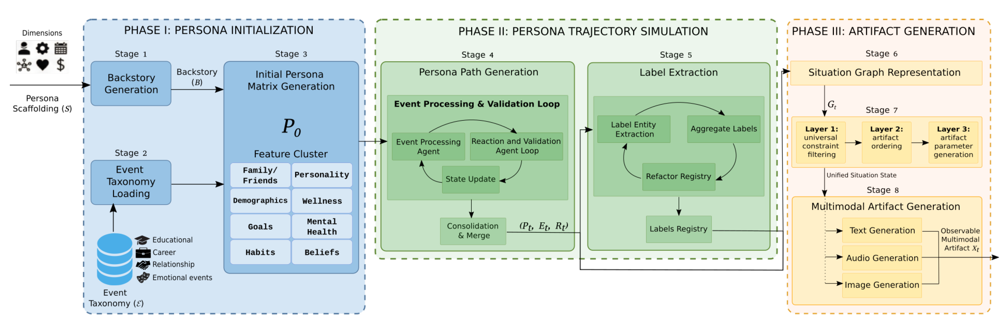
Figure 4.
Temporal stability floor: mean TSCD per archetype over 50 transitions. Dashed line marks the 0.80 reference level. Danielle (Self-centered) shows the most frequent rate-cap violations. Overall mean .
Figure 4.
Temporal stability floor: mean TSCD per archetype over 50 transitions. Dashed line marks the 0.80 reference level. Danielle (Self-centered) shows the most frequent rate-cap violations. Overall mean .
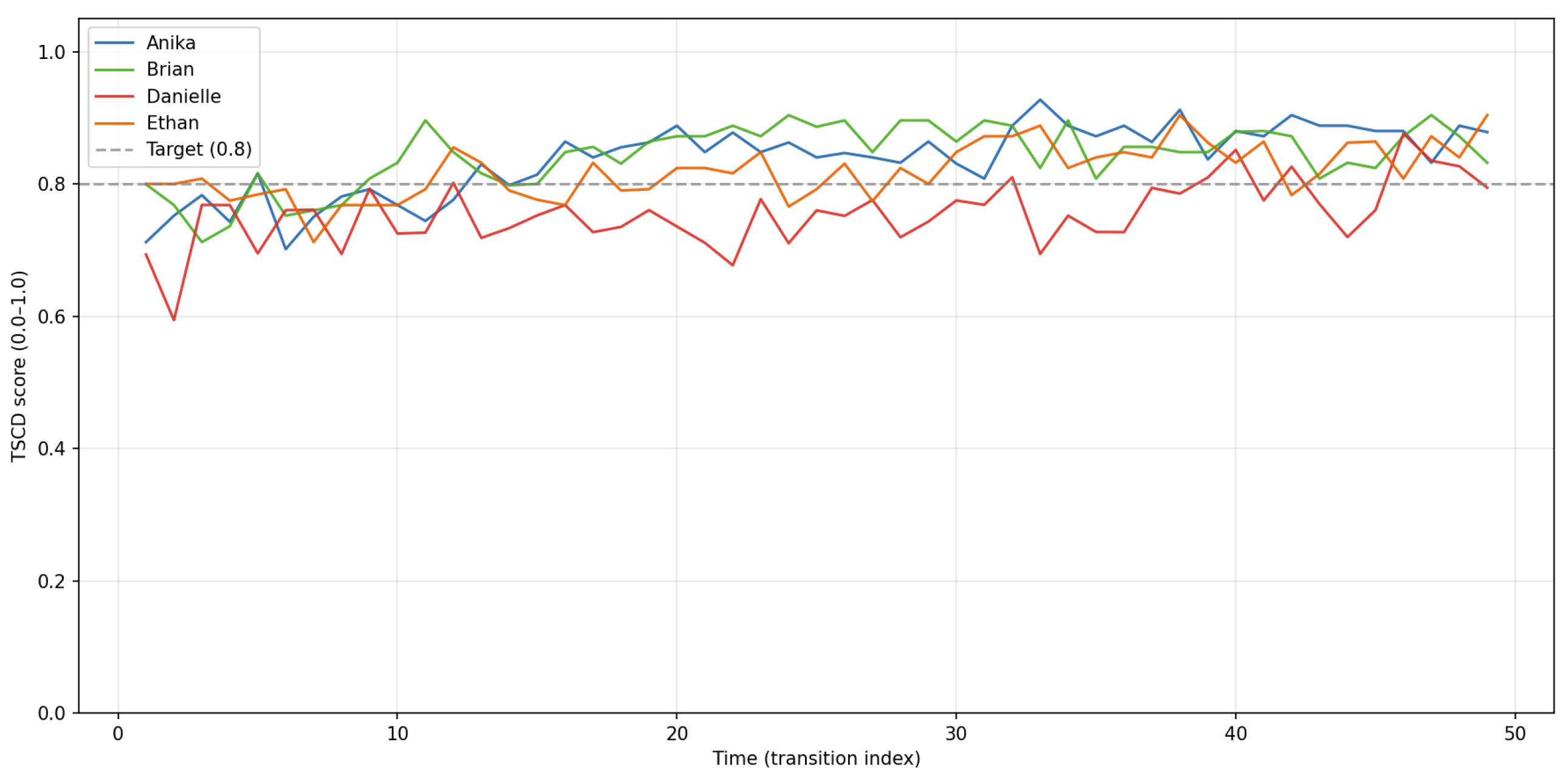
Figure 5.
Inter-class separation over time. Solid lines: pairwise centroid distances; dashed line: mean within-archetype spread. The identity signal persists above stochastic noise throughout, including at the terminal timestep.
Figure 5.
Inter-class separation over time. Solid lines: pairwise centroid distances; dashed line: mean within-archetype spread. The identity signal persists above stochastic noise throughout, including at the terminal timestep.
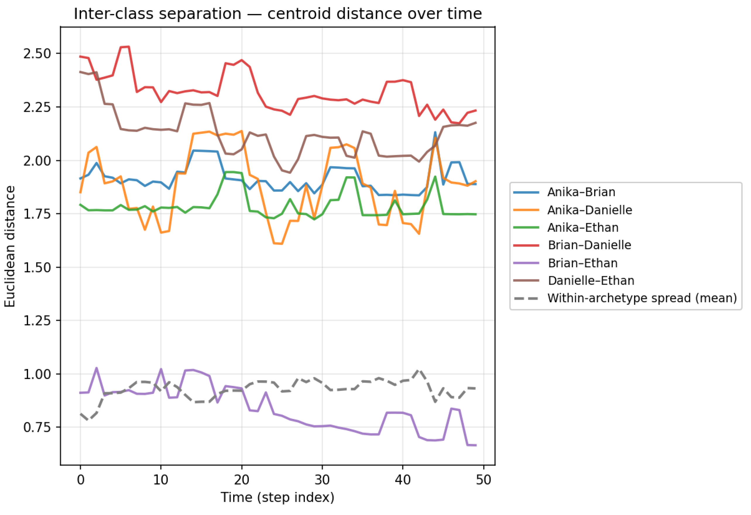
Figure 6.
Identity persistence in state space (t-SNE, perplexity , ). Each point is one timestep-level Persona Matrix (). color encodes archetype. Sub-trajectories from independent seeds form coherent paths within each archetype region. The Brian–Ethan overlap is attributable to shared demographic encodings (Table 4).
Figure 6.
Identity persistence in state space (t-SNE, perplexity , ). Each point is one timestep-level Persona Matrix (). color encodes archetype. Sub-trajectories from independent seeds form coherent paths within each archetype region. The Brian–Ethan overlap is attributable to shared demographic encodings (Table 4).
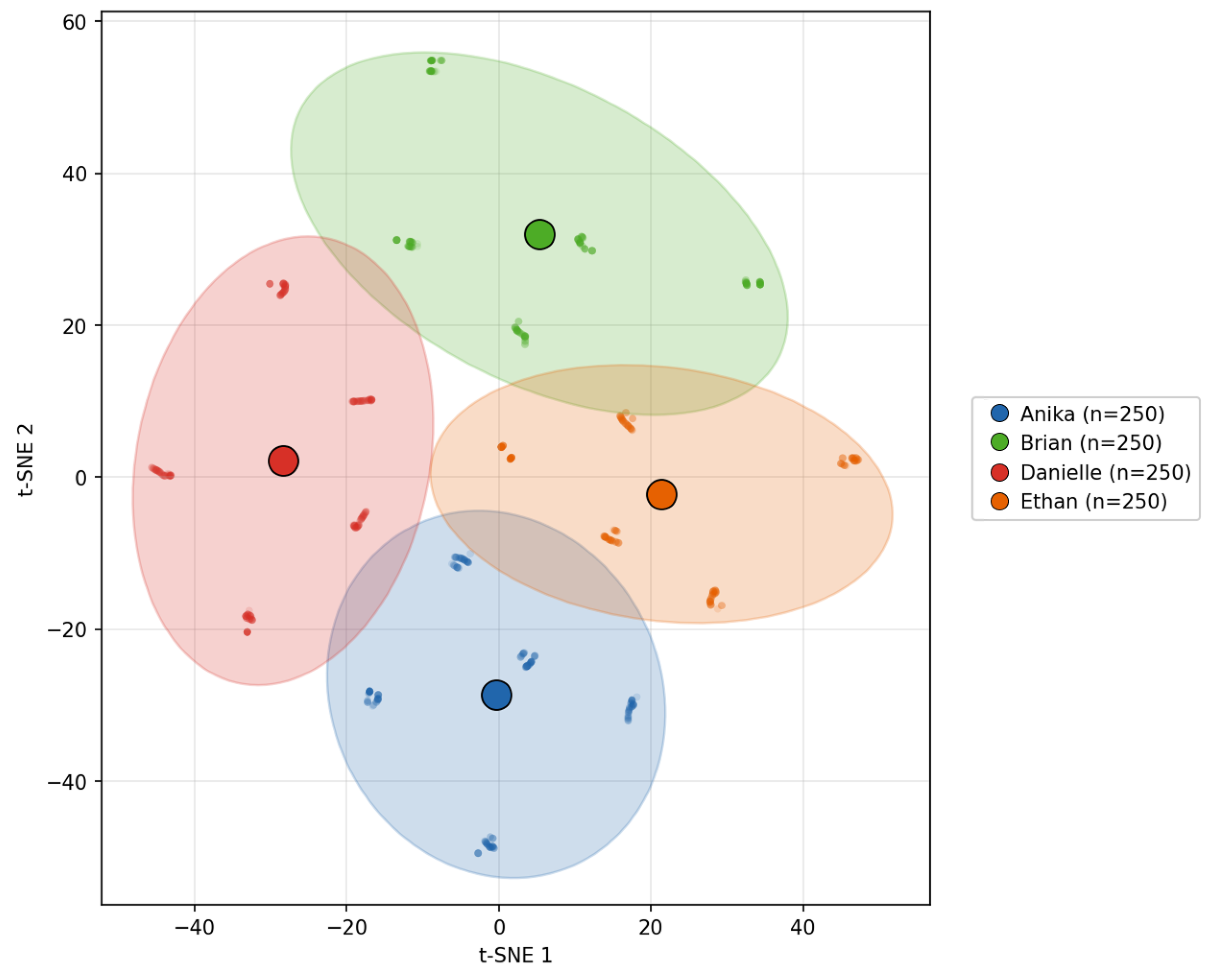
Figure 7.
The coherence frontier under short-horizon (100 events / 100 days, dark) and long-horizon (100 events / 5 years, light) conditions for two archetypes. The short-horizon polygon contracts most strongly on TVS and THC, indicating that the frontier is driven primarily by resolution-sensitive temporal dimensions rather than uniform quality degradation. Danielle’s short-horizon profile is also more distorted than Ethan’s, consistent with higher archetype volatility amplifying compression sensitivity.
Figure 7.
The coherence frontier under short-horizon (100 events / 100 days, dark) and long-horizon (100 events / 5 years, light) conditions for two archetypes. The short-horizon polygon contracts most strongly on TVS and THC, indicating that the frontier is driven primarily by resolution-sensitive temporal dimensions rather than uniform quality degradation. Danielle’s short-horizon profile is also more distorted than Ethan’s, consistent with higher archetype volatility amplifying compression sensitivity.
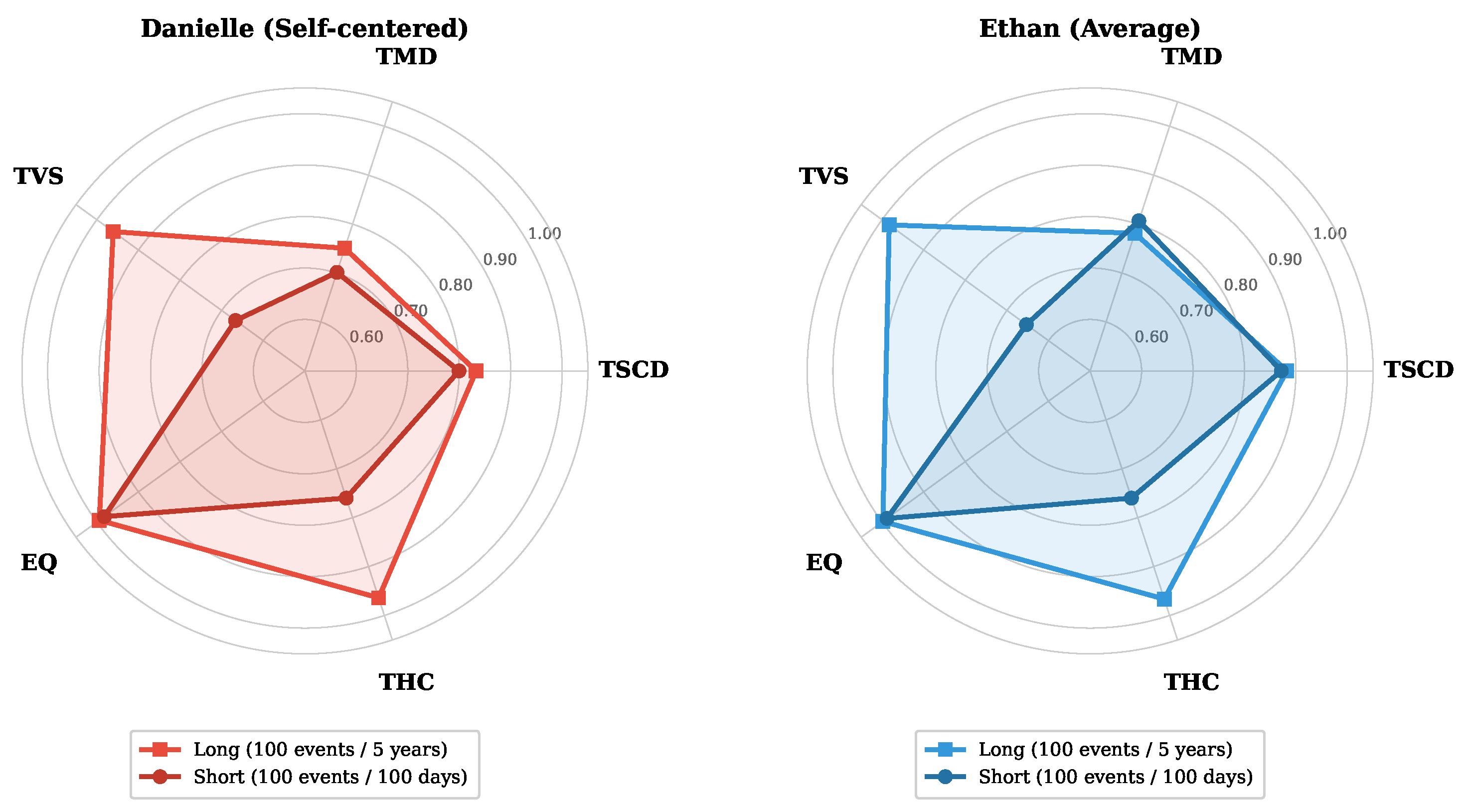
Figure 8.
Experiment 3: Full per-metric breakdown. Color intensity encodes score magnitude (darker = higher). All values are means over seeds. Full numerical results are reported in Table A5 in the Appendix.
Figure 8.
Experiment 3: Full per-metric breakdown. Color intensity encodes score magnitude (darker = higher). All values are means over seeds. Full numerical results are reported in Table A5 in the Appendix.
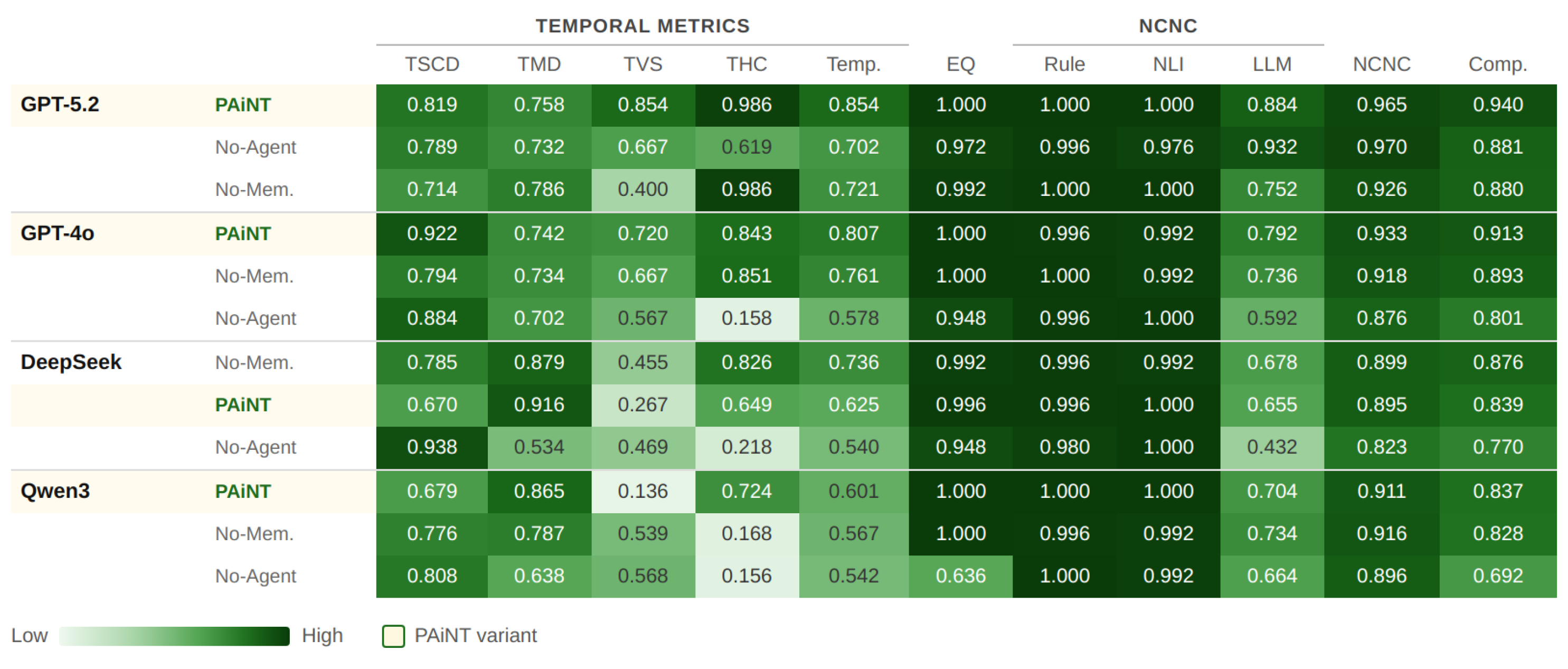
Figure 9.
SGC–SGF relationship by modality. Each point is one archetype–seed run. The positive association indicates that better artifacts tend to be both more comprehensive and more grounded, rather than trading one property off against the other. Text artifacts cluster closest to the upper-right region.
Figure 9.
SGC–SGF relationship by modality. Each point is one archetype–seed run. The positive association indicates that better artifacts tend to be both more comprehensive and more grounded, rather than trading one property off against the other. Text artifacts cluster closest to the upper-right region.
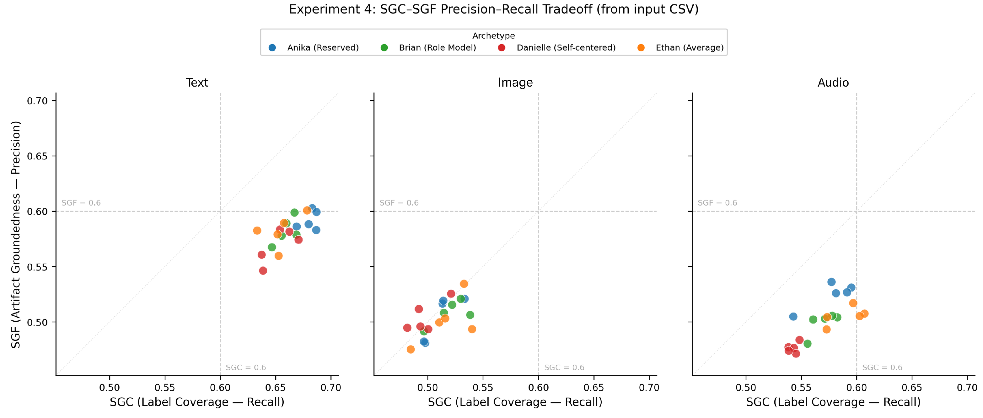
Figure 11.
Distribution of edge types across all 400 PAi-Bench Situation Graphs. Edge types appearing in every graph (has_valence, feels, occurs_during, and core spatiotemporal predicates) approach the maximum of 400 triplets, while social and psychological edges (interacts_with, joins, experiences, conveys_valence) are sparser, reflecting their conditional role in the schema.
Figure 11.
Distribution of edge types across all 400 PAi-Bench Situation Graphs. Edge types appearing in every graph (has_valence, feels, occurs_during, and core spatiotemporal predicates) approach the maximum of 400 triplets, while social and psychological edges (interacts_with, joins, experiences, conveys_valence) are sparser, reflecting their conditional role in the schema.
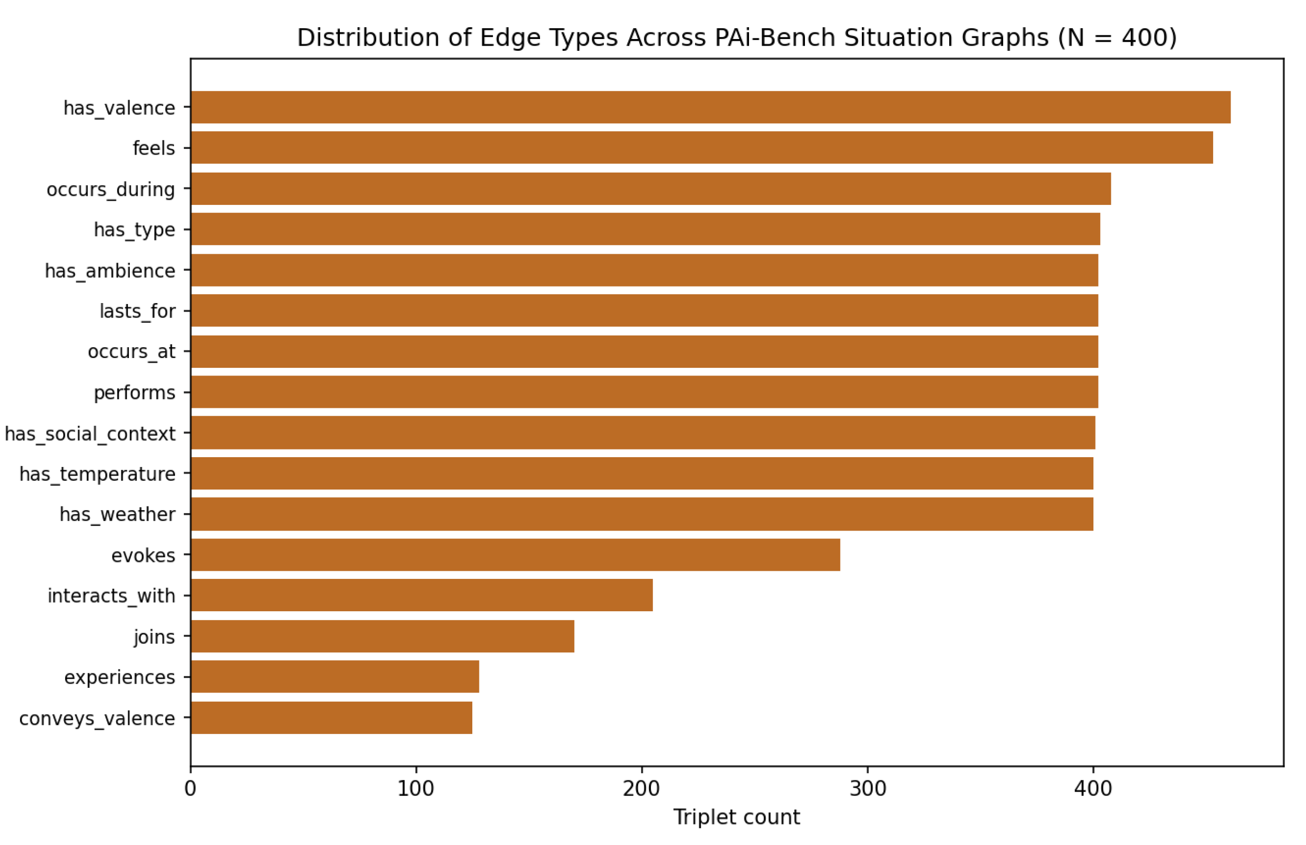
Figure 12.
Distribution of node types by unique (kind, value) pair count across all 400 PAi-Bench Situation Graphs. All required node types approach 400, confirming schema compliance. Participant is the only node type substantially below this ceiling, reflecting its optional and persona-dependent role. The slight excess of Emotion and Valence above 400 indicates that a subset of graphs encodes multiple co-occurring emotional states.
Figure 12.
Distribution of node types by unique (kind, value) pair count across all 400 PAi-Bench Situation Graphs. All required node types approach 400, confirming schema compliance. Participant is the only node type substantially below this ceiling, reflecting its optional and persona-dependent role. The slight excess of Emotion and Valence above 400 indicates that a subset of graphs encodes multiple co-occurring emotional states.
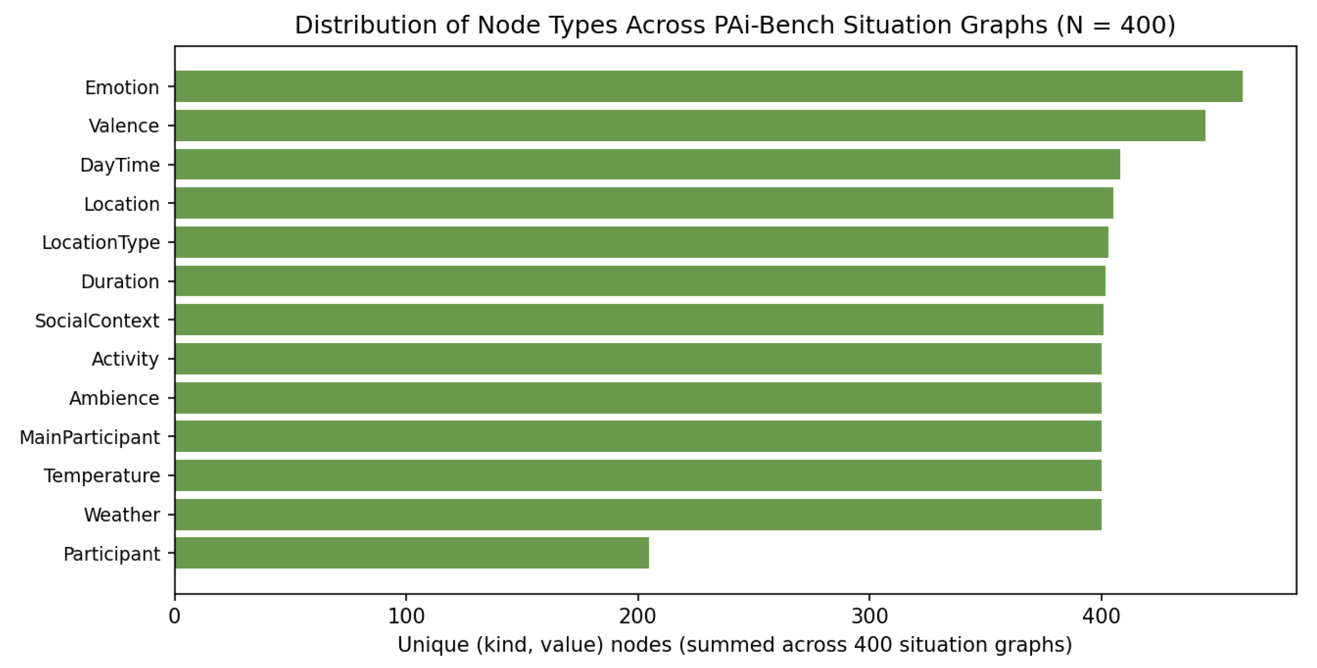
Figure 13.
Top 15 most frequent event titles in PAi-Bench, stacked by archetype ( total event occurrences). A small shared core of life events appears across personas, while the long tail (71 further titles, not shown) captures archetype-specific behavior.
Figure 13.
Top 15 most frequent event titles in PAi-Bench, stacked by archetype ( total event occurrences). A small shared core of life events appears across personas, while the long tail (71 further titles, not shown) captures archetype-specific behavior.
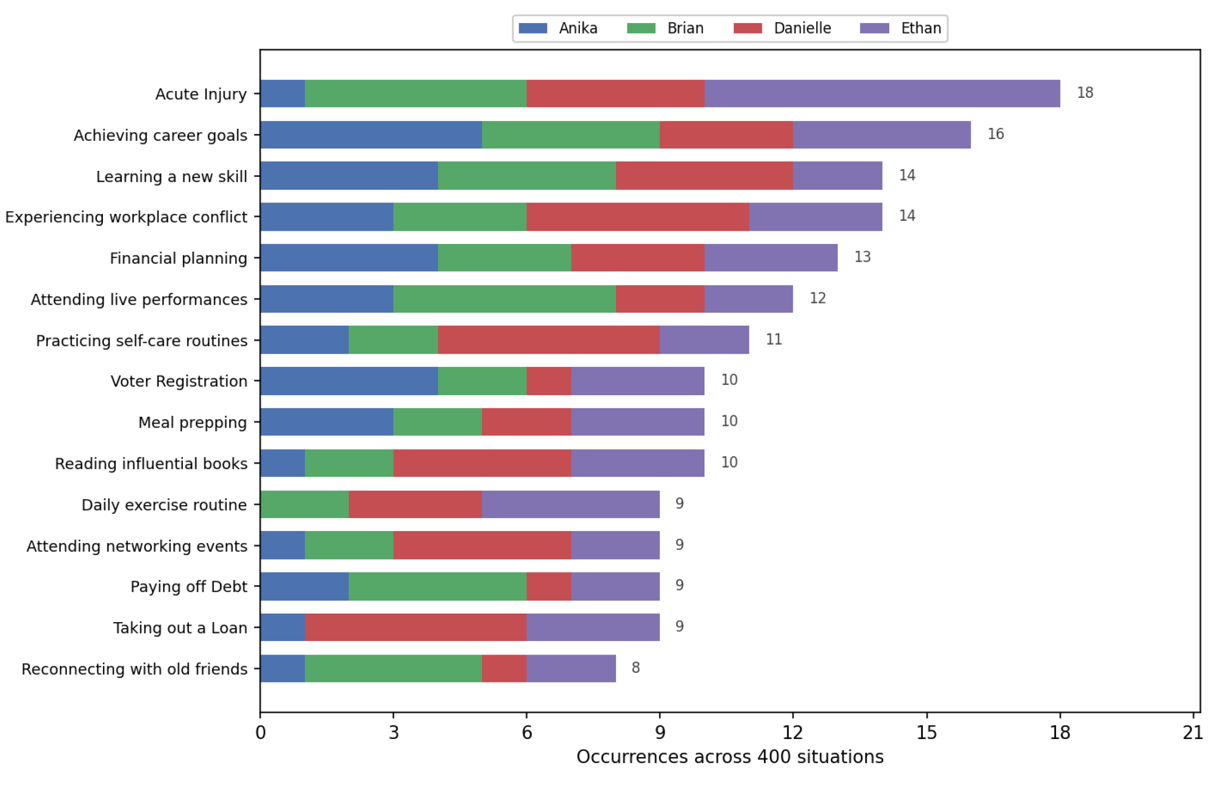
Figure 14.
Event frequency distribution in PAi-Bench, ranked by total occurrences across all 400 situations (80 distinct titles drawn from the 260-event PAiNT taxonomy).
Figure 14.
Event frequency distribution in PAi-Bench, ranked by total occurrences across all 400 situations (80 distinct titles drawn from the 260-event PAiNT taxonomy).
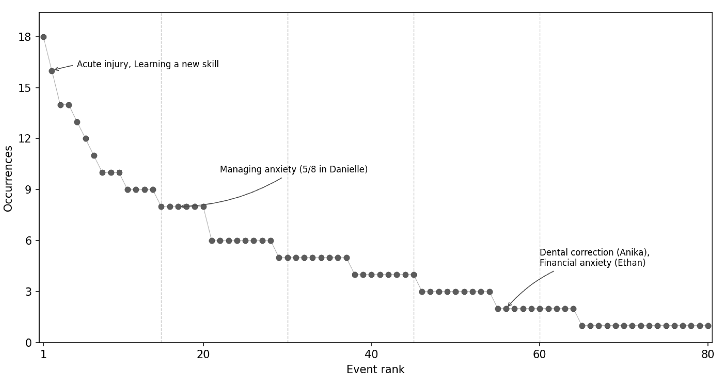
Table 1.
Situation Graph node types (), their type-specific entity enumerations (), and allowed values. Closed: the value is fully determined by . Open: the value is drawn from the finite, persona-specific label registry produced by Stage 5 and populated by the Autolabeler in Stage 6.
Table 1.
Situation Graph node types (), their type-specific entity enumerations (), and allowed values. Closed: the value is fully determined by . Open: the value is drawn from the finite, persona-specific label registry produced by Stage 5 and populated by the Autolabeler in Stage 6.
| Node Type () | Allowed Entities () | Allowed Values |
|---|---|---|
| MainParticipant | {Person} | Open (value from Stage 5) |
| Participant | {FamilyMember, Friend, RomanticPartner, Acquaintance} | Open (value from Stage 5) |
| Activity | {Activity} | Open (value from via Stage 5) |
| Location | {Global, Country, Region, City} | Open (value from Stage 5) |
| LocationType | {Home, Work, School, Park, Restaurant, Cafe, Hotel, Airport, Gym, Beach, Theatre, Museum, Library} | Open (value from Stage 5) |
| DayTime | {Morning, Afternoon, Evening, Night} | Closed (value ) |
| Duration | {Brief, FewHours, HalfDay, FullDay} | Closed (value ) |
| Ambience | {Serene, Cozy, Vibrant, Chaotic, Mysterious, Majestic, Bleak, Romantic, Calm} | Closed (value ) |
| SocialContext | {Intimate, Casual, SemiFormal, Professional, Ceremonial} | Closed (value ) |
| Weather | {Rainy, Sunny, Snowy, Cloudy, Foggy, Windy, Stormy} | Closed (value ) |
| Temperature | {Hot, Warm, Cool, Cold, Freezing} | Closed (value ) |
| Emotion | {Happy, Sad, Fear, Disgust, Anger, Surprise} | Closed (value ) |
| Valence | {Positive, Negative} | Closed (value ) |
Table 2.
Situation Graph constraint map: complete set of valid (source kind → target kind) pairs for each of the 16 edge types. The five semantic edge groups — core action, spatiotemporal, atmospheric, environmental, and psychological — were designed to cover the canonical dimensions of human situation representation identified in cognitive science [36,37].
Table 2.
Situation Graph constraint map: complete set of valid (source kind → target kind) pairs for each of the 16 edge types. The five semantic edge groups — core action, spatiotemporal, atmospheric, environmental, and psychological — were designed to cover the canonical dimensions of human situation representation identified in cognitive science [36,37].
| Semantic Group | Edge Type (p) | Valid |
|---|---|---|
| Core action | performs | MainParticipant → Activity |
| experiences | MainParticipant → Activity; Participant → Activity | |
| joins | Participant → Activity | |
| interacts_with | MainParticipant → Participant; Participant → MainParticipant; Participant → Participant | |
| Spatiotemporal | occurs_at | Activity → Location |
| has_type | Location → LocationType | |
| occurs_during | Activity → DayTime | |
| lasts_for | Activity → Duration | |
| Atmospheric | has_ambience | Activity → Ambience; Location → Ambience |
| has_social_context | Activity → SocialContext; Location → SocialContext | |
| Environmental | has_weather | Activity → Weather |
| has_temperature | Activity → Temperature | |
| Psychological | feels | MainParticipant → Emotion; Participant → Emotion |
| has_valence | Emotion → Valence | |
| evokes | Activity → Emotion | |
| conveys_valence | Activity → Valence |
Table 3.
Summary of the PAiNT evaluation metrics. The suite includes constraint-satisfaction metrics, which function as validity checks, and characterization metrics, which support comparative analysis across experiments.
Table 3.
Summary of the PAiNT evaluation metrics. The suite includes constraint-satisfaction metrics, which function as validity checks, and characterization metrics, which support comparative analysis across experiments.
| Metric | Definition |
|---|---|
| Category: Persona Representation Quality | |
| Structural | |
| OCV: Ontology & Constraint Validity | Checks whether each Persona Matrix satisfies the schema and ontology constraints (field types, value ranges, invariants). |
| Temporal | |
| TSCD: Temporal Smoothness & Controlled Drift | Detects implausibly large per-step attribute changes using calibrated daily rate caps and hard absolute ceilings. |
| TMD: Temporal Macro Drift | Detects generative stagnation by measuring cumulative drift budget utilization for state-like attributes across the full trajectory. |
| TVS: Temporal Volatility Structure | Evaluates whether the distributional pattern of step-level drift activity exhibits realistic variability — neither mechanically uniform nor chaotically erratic. |
| THC: Temporal Horizon Compliance | Evaluates whether the generated trajectory respects the configured simulation horizon, penalizing both temporal undershoot and overshoot with an asymmetric band-pass scoring function. |
| Event-Driven | |
| EQ: Event Quality | Measures the fraction of sampled events that appear in the canonical Event Taxonomy, detecting event hallucination. |
| NCNC: Narrative Coherence & Non-Contradiction | Assesses logical consistency of the event timeline using rule-based prerequisite checks, attribute-scoped NLI contradiction detection, and an LLM-based narrative plausibility audit. |
| Category: Distributional & Stability Diagnostics | |
| Silhouette Score (Inter-Class Separation) | Quantifies how well Persona Matrices cluster by archetype in identity state space using the mean silhouette coefficient. |
| Final-State Spread (Intra-Class Stability) | Measures within-archetype dispersion of terminal identity states across stochastic seeds using mean Euclidean distance to the archetype centroid. |
| Category: Artifact–Graph Alignment | |
| SGC: Situation Graph Consistency | Evaluates whether generated artifacts entail (and do not contradict) facts encoded in the corresponding Situation Graph. |
| SGF: Situation Graph Faithfulness | Evaluates whether facts asserted by generated artifacts are grounded in the corresponding Situation Graph, penalizing contradictions and treating ungrounded elaboration as neutral. |
Table 4.
Pairwise centroid distance decomposition by sub-vector component, sorted by full distance (descending).
Table 4.
Pairwise centroid distance decomposition by sub-vector component, sorted by full distance (descending).
| Pair | Full | Core | Fixed | Narrative |
|---|---|---|---|---|
| Brian–Danielle | 2.279 | 1.440 | 1.727 | 0.369 |
| Danielle–Ethan | 2.087 | 1.086 | 1.746 | 0.375 |
| Anika–Brian | 1.881 | 0.829 | 1.651 | 0.356 |
| Anika–Danielle | 1.846 | 1.313 | 1.254 | 0.355 |
| Anika–Ethan | 1.755 | 0.533 | 1.648 | 0.282 |
| Brian–Ethan | 0.754 | 0.604 | 0.328 | 0.306 |
Table 5.
Experiment 1 summary. All trajectories generated with GPT-5.2.
| Per-Archetype | ||||||
|---|---|---|---|---|---|---|
| Metric | Claims | Overall | Anika | Brian | Danielle | Ethan |
| TSCD | C1 | 0.814 | 0.838 | 0.843 | 0.755 | 0.819 |
| Silhouette Score | C2 | 0.269 | 0.273 | 0.113 | 0.443 | 0.246 |
| Final Spread | C3 | 0.932 | 1.138 | 0.881 | 0.961 | 0.746 |
Table 6.
Experiment 2: Mean metric scores by archetype and horizon ( seeds per condition). All generated with GPT-5.2.
Table 6.
Experiment 2: Mean metric scores by archetype and horizon ( seeds per condition). All generated with GPT-5.2.
| Archetype | Horizon | TSCD | TMD | TVS | EQ | THC | Composite |
|---|---|---|---|---|---|---|---|
| Danielle | short | 0.800 ± 0.02 | 0.701 ± 0.11 | 0.667 ± 0.00 | 0.982 ± 0.01 | 0.760 ± 0.00 | 0.818 ± 0.02 |
| Danielle | long | 0.833 ± 0.03 | 0.751 ± 0.11 | 0.961 ± 0.09 | 0.994 ± 0.01 | 0.964 ± 0.01 | 0.917 ± 0.02 |
| Ethan | short | 0.872 ± 0.03 | 0.807 ± 0.01 | 0.653 ± 0.02 | 0.988 ± 0.01 | 0.760 ± 0.00 | 0.846 ± 0.01 |
| Ethan | long | 0.882 ± 0.02 | 0.781 ± 0.04 | 0.983 ± 0.02 | 0.998 ± 0.00 | 0.966 ± 0.01 | 0.935 ± 0.01 |
Table 7.
Experiment 2: Conditions ranked by Composite score.
| Rank | Horizon | Persona | Composite |
|---|---|---|---|
| 1 | long | Ethan | 0.935 |
| 2 | long | Danielle | 0.917 |
| 3 | short | Ethan | 0.846 |
| 4 | short | Danielle | 0.818 |
Table 8.
Experiment 2: NCNC scores by archetype and horizon (mean ± std, ). All generated with GPT-5.2.
Table 8.
Experiment 2: NCNC scores by archetype and horizon (mean ± std, ). All generated with GPT-5.2.
| Rule | NLI | LLM | Combined | ||||||
|---|---|---|---|---|---|---|---|---|---|
| Archetype | Horizon | mean | std | mean | std | mean | std | mean | std |
| Danielle | long | 1.000 | 0.00 | 0.998 | 0.00 | 0.932 | 0.05 | 0.979 | 0.01 |
| Danielle | short | 0.998 | 0.00 | 0.994 | 0.01 | 0.790 | 0.12 | 0.934 | 0.04 |
| Ethan | long | 0.998 | 0.00 | 0.988 | 0.01 | 0.870 | 0.09 | 0.956 | 0.02 |
| Ethan | short | 1.000 | 0.00 | 0.990 | 0.01 | 0.836 | 0.10 | 0.947 | 0.03 |
Table 9.
Experiment 3: Summary scores sorted by Composite. Shaded rows indicate PAiNT (full pipeline).
Table 9.
Experiment 3: Summary scores sorted by Composite. Shaded rows indicate PAiNT (full pipeline).
| Model | Variant | Temporal | EQ | NCNC | Composite |
|---|---|---|---|---|---|
| GPT-5.2 | PAiNT | 0.854 ± 0.02 | 1.000 ± 0.00 | 0.965 ± 0.02 | 0.940 ± 0.01 |
| GPT-4o | PAiNT | 0.807 ± 0.06 | 1.000 ± 0.00 | 0.933 ± 0.03 | 0.913 ± 0.02 |
| GPT-4o | No-Memory | 0.761 ± 0.03 | 1.000 ± 0.00 | 0.918 ± 0.03 | 0.893 ± 0.01 |
| GPT-5.2 | No-Agent | 0.702 ± 0.04 | 0.972 ± 0.02 | 0.970 ± 0.02 | 0.881 ± 0.02 |
| GPT-5.2 | No-Memory | 0.721 ± 0.02 | 0.992 ± 0.01 | 0.926 ± 0.02 | 0.880 ± 0.01 |
| DeepSeek | No-Memory | 0.736 ± 0.05 | 0.992 ± 0.02 | 0.899 ± 0.04 | 0.876 ± 0.02 |
| DeepSeek | PAiNT | 0.626 ± 0.05 | 0.996 ± 0.01 | 0.895 ± 0.08 | 0.839 ± 0.03 |
| Qwen3 | PAiNT | 0.601 ± 0.04 | 1.000 ± 0.00 | 0.911 ± 0.03 | 0.837 ± 0.02 |
| Qwen3 | No-Memory | 0.567 ± 0.04 | 1.000 ± 0.00 | 0.916 ± 0.03 | 0.828 ± 0.02 |
| GPT-4o | No-Agent | 0.578 ± 0.03 | 0.948 ± 0.05 | 0.876 ± 0.03 | 0.801 ± 0.02 |
| DeepSeek | No-Agent | 0.540 ± 0.07 | 0.948 ± 0.06 | 0.823 ± 0.05 | 0.770 ± 0.04 |
| Qwen3 | No-Agent | 0.542 ± 0.03 | 0.636 ± 0.17 | 0.896 ± 0.06 | 0.691 ± 0.06 |
Table 10.
Experiment 4: Situation Graph OCV by archetype (mean ± std, ). Graphs generated with GPT-5.2.
Table 10.
Experiment 4: Situation Graph OCV by archetype (mean ± std, ). Graphs generated with GPT-5.2.
| Archetype | OCV (mean) | OCV (std) |
|---|---|---|
| Anika (Reserved) | 0.824 | 0.037 |
| Brian (Role Model) | 0.810 | 0.039 |
| Danielle (Self-centered) | 0.820 | 0.041 |
| Ethan (Average) | 0.822 | 0.041 |
| Overall | 0.819 | 0.040 |
Table 11.
Experiment 4: SGC by archetype and modality (mean ± std, ). The Mean row reports the cross-archetype mean for each modality.
Table 11.
Experiment 4: SGC by archetype and modality (mean ± std, ). The Mean row reports the cross-archetype mean for each modality.
| Archetype | Text | Image | Audio |
|---|---|---|---|
| Anika | 0.681 ± 0.08 | 0.511 ± 0.13 | 0.577 ± 0.10 |
| Brian | 0.659 ± 0.09 | 0.518 ± 0.13 | 0.570 ± 0.10 |
| Danielle | 0.655 ± 0.10 | 0.498 ± 0.12 | 0.543 ± 0.10 |
| Ethan | 0.655 ± 0.10 | 0.517 ± 0.12 | 0.590 ± 0.08 |
| Mean | 0.662 ± 0.02 | 0.511 ± 0.02 | 0.570 ± 0.02 |
Table 12.
Experiment 4: SGF by archetype and modality (mean ± std, ). The Mean row reports the cross-archetype mean for each modality.
Table 12.
Experiment 4: SGF by archetype and modality (mean ± std, ). The Mean row reports the cross-archetype mean for each modality.
| Archetype | Text | Image | Audio |
|---|---|---|---|
| Anika | 0.592 ± 0.08 | 0.503 ± 0.11 | 0.525 ± 0.09 |
| Brian | 0.581 ± 0.09 | 0.509 ± 0.12 | 0.499 ± 0.10 |
| Danielle | 0.575 ± 0.10 | 0.501 ± 0.10 | 0.478 ± 0.10 |
| Ethan | 0.583 ± 0.11 | 0.501 ± 0.10 | 0.506 ± 0.09 |
| Mean | 0.582 ± 0.02 | 0.505 ± 0.02 | 0.502 ± 0.02 |
Table 13.
Experiment 4: SGF verdict distribution by modality (% of artifact triplets).
| Modality | Positive TE (%) | Non TE (%) | Negative TE (%) | N |
|---|---|---|---|---|
| Text | 31.3 | 53.4 | 15.3 | 12,960 |
| Image | 19.8 | 59.3 | 20.9 | 21,606 |
| Audio | 18.0 | 64.8 | 17.3 | 12,635 |
| Overall | 22.5 | 59.2 | 18.4 | 47,201 |
Table 14.
Estimated per-run cost for the persona simulation phase of 50 timesteps (Stages 1–4) under the full PAiNT configuration. Token counts are means over seeds. Costs are calculated as .
Table 14.
Estimated per-run cost for the persona simulation phase of 50 timesteps (Stages 1–4) under the full PAiNT configuration. Token counts are means over seeds. Costs are calculated as .
| Model | Input (M) | Output (M) | Est. Cost (USD) | Time (min) |
|---|---|---|---|---|
| GPT-5.2 | 3.341 | 0.369 | $11.01 | 95.11 |
| GPT-4o | 2.364 | 0.209 | $7.99 | 42.04 |
| DeepSeek-V3 | 2.570 | 0.188 | $4.00 | 125.15 |
| Qwen3-235B-A22B | 3.332 | 0.346 | $1.25 | 193.62 |
| Served via the Replicate API; proprietary models served via the OpenAI API. | ||||
Table 15.
Per-run token and runtime footprint by backbone and architectural variant from Experiment 3 (§ Section 6.4) ( seeds). Shaded rows correspond to the full PAiNT pipeline. This table quantifies the computational overhead of orchestration and memory relative to the ablated variants.
Table 15.
Per-run token and runtime footprint by backbone and architectural variant from Experiment 3 (§ Section 6.4) ( seeds). Shaded rows correspond to the full PAiNT pipeline. This table quantifies the computational overhead of orchestration and memory relative to the ablated variants.
| Model | Variant | Input (M) | Output (M) | Time (min) |
|---|---|---|---|---|
| GPT-5.2 | PAiNT | 3.341 | 0.369 | 95.11 |
| GPT-5.2 | No-Memory | 1.822 | 0.375 | 90.20 |
| GPT-5.2 | No-Agent | 0.552 | 0.141 | 26.32 |
| GPT-4o | PAiNT | 2.364 | 0.209 | 42.04 |
| GPT-4o | No-Memory | 1.318 | 0.219 | 56.30 |
| GPT-4o | No-Agent | 0.370 | 0.059 | 9.60 |
| DeepSeek | PAiNT | 2.570 | 0.188 | 125.15 |
| DeepSeek | No-Memory | 1.306 | 0.216 | 124.73 |
| DeepSeek | No-Agent | 0.371 | 0.069 | 26.40 |
| Qwen3 | PAiNT | 3.332 | 0.346 | 193.62 |
| Qwen3 | No-Memory | 1.537 | 0.343 | 178.14 |
| Qwen3 | No-Agent | 0.530 | 0.139 | 75.14 |
Table 16.
Resource consumption and estimated cost for the full PAiNT pipeline (Stages 1–8) using GPT-5.2. Values represent both the aggregate and mean across 20 complete persona trajectories.
Table 16.
Resource consumption and estimated cost for the full PAiNT pipeline (Stages 1–8) using GPT-5.2. Values represent both the aggregate and mean across 20 complete persona trajectories.
| Metric | Input (M) | Output (M) | Cost (USD) | Time (min) |
|---|---|---|---|---|
| Total (20 runs) | 111.190 | 13.264 | $380.28 | 4,202.84 |
| Mean per run | 5.560 | 0.663 | $19.01 | 210.14 |
Table 17.
Situation Graph structural statistics per archetype on PAi-Bench ( graphs per archetype, 400 total). Nodes are counted as unique (kind, value) pairs appearing as a subject or object of at least one triplet.
Table 17.
Situation Graph structural statistics per archetype on PAi-Bench ( graphs per archetype, 400 total). Nodes are counted as unique (kind, value) pairs appearing as a subject or object of at least one triplet.
| Archetype | N graphs | Min | Max | Mean | Median |
|---|---|---|---|---|---|
| Anika | 100 | 09 | 19 | 12.59 | 12 |
| Brian | 100 | 12 | 15 | 12.77 | 13 |
| Danielle | 100 | 12 | 19 | 12.24 | 13 |
| Ethan | 100 | 12 | 15 | 12.72 | 13 |
| Overall | 400 | 9 | 19 | 12.83 | 13 |
Table 18.
PAi-Bench reproduction cost per archetype (100-event trajectory). LLM cost is computed as using the GPT-5.2 endpoint rates in effect as of April 2026. Non-token image and audio generation costs are excluded.
Table 18.
PAi-Bench reproduction cost per archetype (100-event trajectory). LLM cost is computed as using the GPT-5.2 endpoint rates in effect as of April 2026. Non-token image and audio generation costs are excluded.
| Archetype | Duration (h) | Input (M) | Output (M) | LLM cost (USD) |
|---|---|---|---|---|
| Anika | 06.36 | 10.61 | 1.24 | $35.88 |
| Brian | 06.69 | 11.25 | 1.32 | $38.18 |
| Danielle | 08.10 | 11.97 | 1.41 | $40.71 |
| Ethan | 06.64 | 11.13 | 1.28 | $37.41 |
| Total | 27.80 | 44.96 | 5.25 | $152.18 |
Table 19.
Zero-shot SGP performance on PAi-Bench (, ).
| Metric | Gemini 2.5 Flash | Claude Sonnet 4 | Qwen3-235B |
|---|---|---|---|
| Strict Exact Match | |||
| Precision | |||
| Recall | |||
| F1 | |||
| Soft Semantic Match | |||
| Precision | |||
| Recall | |||
| F1 | |||
| Structural Compliance | |||
| PVR ↓ | |||
| Prediction Volume | |||
| Triples/event | |||
Table 20.
Per-persona zero-shot SGP: Strict F1 and Soft F1 across models ( per persona).
| Anika | Brian | Danielle | Ethan | Overall | ||||||
|---|---|---|---|---|---|---|---|---|---|---|
| Model | Strict | Soft | Strict | Soft | Strict | Soft | Strict | Soft | Strict | Soft |
| Gemini 2.5 Flash | .056 | .158 | .044 | .139 | .053 | .141 | .050 | .156 | .051 | .149 |
| Claude Sonnet 4 | .058 | .186 | .045 | .168 | .046 | .156 | .050 | .176 | .050 | .171 |
| Qwen3-235B | .061 | .149 | .045 | .108 | .046 | .112 | .062 | .137 | .054 | .126 |
Disclaimer/Publisher’s Note: The statements, opinions and data contained in all publications are solely those of the individual author(s) and contributor(s) and not of MDPI and/or the editor(s). MDPI and/or the editor(s) disclaim responsibility for any injury to people or property resulting from any ideas, methods, instructions or products referred to in the content. |
© 2026 by the authors. Licensee MDPI, Basel, Switzerland. This article is an open access article distributed under the terms and conditions of the Creative Commons Attribution (CC BY) license (http://creativecommons.org/licenses/by/4.0/).
Copyright: This open access article is published under a Creative Commons CC BY 4.0 license, which permit the free download, distribution, and reuse, provided that the author and preprint are cited in any reuse.


