

Submitted:
24 May 2026
Posted:
25 May 2026
You are already at the latest version
Abstract
Electric vehicle routing problems (EVRPs) have become increasingly important in sustainable logistics, where routing decisions must account for limited battery capacity, charging constraints, and time windows. In such settings, fast and adaptive decision-making is critical. Nature-inspired genetic programming (GP)-based hyper-heuristics, particularly those based on routing policies, offer a promising approach by evolving decision rules through mechanisms analogous to biological evolution, enabling adaptive behavior in dynamic environments. However, existing GP-based approaches have been developed for deterministic routing settings, limiting their applicability in real-world environments characterized by uncertainty. This work extends a GP-based route generation scheme (RGS) framework to a stochastic electric vehicle routing problem with time windows (EVRPTW) setting by incorporating variability in customer demand, service time, and travel time through controlled stochastic perturbations. The priority function representation is extended with additional terminals capturing stochastic effects and global system information, and new variants of existing routing strategies are introduced to improve robustness through capacity-aware vehicle selection. The proposed method is evaluated across a range of stochastic scenarios and objectives, including fleet size, energy consumption, and total tardiness. The results demonstrate that different routing strategies are best suited to different optimization objectives, with each approach consistently exhibiting strengths aligned with specific performance criteria, while stochasticity primarily amplifies these structural differences rather than altering their relative behavior. These findings further support the suitability of evolutionary, nature-inspired approaches for constructing adaptive decision policies in stochastic routing environments.
Keywords:
electric vehicle routing problem
; stochastic vehicle routing
; routing policies
; genetic programming
; hyper-heuristics
; evolutionary computation
; nature-inspired optimization
1. Introduction
The vehicle routing problem (VRP) is a fundamental combinatorial optimization problem that has been extensively studied in the operations research literature [1]. Its practical relevance arises from a wide range of applications in transportation, logistics, and production systems [2]. Over time, numerous variants have been developed to better reflect operational constraints, including the vehicle routing problem with time windows (VRPTW) and pickup-and-delivery settings [3,4].
In the context of sustainable transportation, electric vehicle routing problems (EVRPs) have received increasing attention [5,6,7]. In these problems, routing decisions must consider not only customer service requirements, but also battery capacity, charging time, and charging infrastructure constraints. In particular, logistics systems using electric vehicles must explicitly address limited driving ranges and the need for recharging along routes, which is especially critical in mid- and long-haul operations [8].
An important development in EVRP research is the electric vehicle routing problem with time windows (EVRPTW) introduced i n [9], which extends the classical Solomon benchmark framework [10] and has become the standard reference model. Despite substantial progress in EVRPTW, most existing approaches rely on deterministic assumptions, where customer demand, travel times, and service durations are known in advance [11,12,13].
In practice, routing systems are inherently stochastic, with uncertainty in demand, travel time, and service duration, all of which can significantly affect routing decisions. Such sources of uncertainty have been recognized in the stochastic VRP literature [14,15], yet their integration into EV routing remains limited, with existing approaches typically relying on stochastic programming, simulation, or reinforcement learning frameworks [16,17,18]. Although expressive, these methods are computationally demanding and less suitable for fast or real-time decision-making. Recent work continues to explore how uncertainty can be modeled and incorporated into EV routing, highlighting that this remains an open and actively researched problem [19].
A complementary direction is provided by recent GP-based hyper-heuristic approaches for EVRPTW [20], which generate routing policies via a route generation scheme (RGS) instead of relying on iterative solution improvement, enabling fast and adaptive decision-making. However, such approaches have so far been developed only under deterministic assumptions, leaving a gap between stochastic modeling and policy-based routing.
Genetic programming, as a form of evolutionary computation, is directly inspired by biological evolution, where populations of candidate solutions evolve through selection, variation, and inheritance [21]. These mechanisms enable the emergence of adaptive behaviors without explicit design, reflecting how natural systems respond to changing environments. In the context of routing under uncertainty, this perspective is particularly relevant, as effective solutions must continuously adapt to evolving conditions rather than rely on fixed plans.
This paper addresses this gap by extending the GP-based RGS framework to stochastic EVRPTW, incorporating uncertainty in customer demand, travel time, and service duration while retaining the standard Schneider-based problem structure. The proposed approach introduces stochastic variants of the route generation scheme and extends the GP representation to support decision-making under uncertainty.
The main contributions of this work are as follows:
- Two extensions of the route generation scheme (RGS), namely Semi-parallel-B and Parallel-B, are introduced. These variants incorporate candidate-based vehicle selection to improve robustness under stochastic demand conditions.
- The GP-based priority function representation is extended with stochastic and global-state descriptors, as well as objective-specific terminals such as and .
- A stochastic adaptation of the Schneider EVRPTW benchmark instances is developed, incorporating controlled variability in demand, service time, and travel time while preserving the original problem structure.
- A systematic experimental evaluation is conducted across multiple stochastic scenarios and objectives, analyzing the impact of uncertainty on routing performance and comparing different RGS variants.
The remainder of this paper is organized as follows. Section 2 reviews related work on electric vehicle routing and GP-based hyper-heuristics. Section 3 presents the proposed methodology, including the stochastic problem setting, the routing policy framework, and the GP-based approach for evolving priority functions. Section 4 describes the experimental setup and reports the computational results across different objectives and stochastic scenarios. Section 5 discusses the observed behavior of the routing strategies and their interaction with uncertainty. Finally, Section 6 concludes the paper and outlines directions for future research.
2. Related Work
The electric vehicle routing problem with time windows was introduced by [9] as an extension of the classical VRPTW benchmark from [10], incorporating electric vehicle constraints such as limited battery capacity and charging requirements, and has since become the standard reference in the field.b
Most existing work in this domain assumes deterministic problem parameters and relies on metaheuristic optimization methods, particularly adaptive large neighborhood search (ALNS) [11,22,23], iterative local search (ILS) [12], and variable neighborhood search (VNS) [13]. In addition, exact and hybrid methods have also been proposed, including column generation and branch-and-price-based approaches [24,25,26,27,28,29].
In contrast to deterministic formulations, stochastic vehicle routing problems explicitly model uncertainty in key parameters. Early work [30] established fundamental properties of routing with stochastic demands, including the distinction between full and split delivery and different modes of information revelation. A comprehensive overview of stochastic routing variants, including stochastic customers, stochastic demands, and stochastic travel times, is provided in [14]. Similarly, stochastic VRP is classified into three main classes: stochastic customers, stochastic demands, and stochastic times [15]. The authors also discuss solution approaches such as chance-constrained programming and stochastic programming with recourse. These frameworks typically follow a two-stage structure, where an initial solution is constructed before uncertainty is realized, followed by corrective actions once stochastic information becomes available.
Several works have addressed specific stochastic VRP variants. In [31] routing problems with stochastic travel and service times were studied, while in [32] the authors investigated stochastic travel times using branch-and-cut approaches combined with sampling. For stochastic demands, exact and decomposition-based methods were proposed in [33,34], and reinforcement learning approaches were explored in [35]. Although these studies provide important theoretical insights, they are generally based on exact optimization, decomposition, or scenario-based modeling, which limits their applicability in large-scale or real-time settings.
Compared to the classical VRP, stochastic extensions of EVRP and EVRPTW are relatively limited and typically focus on specific sources of uncertainty. For example, stochastic waiting times at charging stations were introduced [16], which modelled waiting time as a random variable revealed upon arrival. Other works consider stochastic customer demand and dynamic routing decisions. In [17] the authors studied EVRP with stochastic demands and dynamic remedial measures using a mixed-integer programming framework, while in [18] the authors addressed a dynamic stochastic EVRP using reinforcement learning. More recent contributions extend stochastic modeling to additional EV-specific factors: in [19] a stochastic electric vehicle location–routing problem incorporating demand uncertainty and environmental effects such as ambient temperature was considered, while in [36] stochastic energy consumption using a two-stage stochastic programming approach with recourse policies was modeled. Despite capturing important real-world aspects, these approaches rely on scenario-based optimization and computationally intensive methods, which limits their applicability in fast or real-time decision-making settings.
Overall, both deterministic metaheuristics and stochastic optimization approaches typically rely on computationally demanding procedures and fixed or scenario-based solution structures, making them less suitable for dynamic environments that require fast and adaptive decision-making. This limitation motivates the exploration of alternative solution paradigms.
Constructive heuristics represent an alternative class of methods that build solutions incrementally rather than improving an existing one. They are commonly used to generate initial solutions or to repair partial solutions within hybrid frameworks. Due to their relatively low computational cost, constructive methods are particularly suitable for dynamic and real-time environments. However, designing effective constructive heuristics is non-trivial, and such approaches are often less explored compared to improvement-based metaheuristics [37].
Genetic programming (GP) [21] has been increasingly used for automatic design of heuristics, particularly in scheduling [38,39] and graph-based optimization problems [40,41]. In the context of vehicle routing, however, its application remains limited. In [42] GP was for the first time used to generate heuristics for VRP. More specifically, the authors considered a dynamic variant of the problem in which customers arrive over time and can be accepted or rejected. The experimental results demonstrate that GP evolved heuristics achieve significantly better results compared to manually designed ones. A similar problem was also considered in [43], in which problems with different levels of dynamic customer arrivals were considered. The results again demonstrated that GP evolved heuristics performed better compared to the manually designed nearest neighbor heuristic. In [41] the authors considered a completely different problem variant, namely VRP with zone-based pricing. This variant models the situation in which profit needs to be maximized by determining which customers should be served. The results demonstrated that GP evolved heuristics achieved better results compared to a genetic algorithm, and were even competitive to a branch & price algorithm, thus outlining the suitability of GP for evolving heuristics for different problem variants.
One of the first notable applications of a GP-based hyper-heuristic framework for EVRPTW was done in [20]. This approach combines GP with a route generation scheme (RGS) to evolve routing policies instead of directly optimizing complete solutions. This shifts the focus from solution search to heuristic generation, enabling faster decision-making and improved adaptability in dynamic settings. This methodology has been further extended by using surrogate models to improve the performance of GP, as well as its convergence [44].
Overall, GP-based approaches provide an efficient and adaptive alternative to traditional EVRPTW solution methods, as they learn routing policies that can be applied quickly in dynamic settings. However, all the previous applications of GP on VRP or EVRP have been done on deterministic problem settings, completely disregarding the uncertainty that can be present in such problems. This highlights the need for extending this methodology further to also cover stochastic variants of the EVRP problem. This adaptive capability reflects the underlying evolutionary principles from which GP originates, making it particularly suitable for decision-making in dynamic and uncertain environments.
3. Materials and Methods
3.1. Electric Vehicle Routing Problem with Time Windows
EVRPTW extends the classical VRP by considering electric vehicles and time-constrained service at customers. The formulation introduced by [9] has become the standard reference model, and most existing EVRPTW studies are based on this framework. Each customer must be serviced within a predefined time window, while routing decisions are constrained by limited battery capacity, energy consumption, and recharging requirements. In contrast to conventional vehicles, battery recharging is significantly slower than refueling, which introduces additional temporal constraints and complicates route planning. As a result, routing decisions involve not only customer assignment and sequencing, but also battery feasibility, charging scheduling, and strict adherence to customer time windows.
The problem is defined on a fully connected symmetric graph , where nodes represent the depot, customers, and charging stations. A single depot is assumed, serving as both the start and end location for all routes. Each link is associated with a distance , which determines the corresponding travel time, while energy consumption is assumed proportional to traveled distance.
To formally define the EVRPTW setting considered in this work, the following notation is used:
: set of customer nodes;
: set of charging-station nodes;
0: depot node;
: set of all nodes;
: distance between nodes i and j;
: nominal demand of customer i;
: nominal service time of customer i;
: service time window associated with customer i;
C: vehicle cargo capacity;
Q: vehicle battery capacity;
v: nominal vehicle speed;
r: energy-consumption rate;
g: charging rate;
: arrival time at customer i;
: completion time of service at customer i;
: tardiness at customer i, defined as .
Each customer must be serviced exactly once by a single vehicle, prohibiting split deliveries. Service at customer requires service duration and must be performed within the associated time window , where denotes the earliest allowable service start time and denotes the due time. Vehicles arriving before must wait until service can begin. Depending on the formulation, time windows may be treated as either hard, where late arrivals are infeasible, or soft, where late service is permitted but penalized.
A homogeneous fleet of vehicles is available at the depot. Each vehicle has cargo capacity C, battery capacity Q, and travels at nominal speed v. Vehicles depart from the depot fully loaded and fully charged. Cargo capacity decreases as customers are served and cannot be replenished during route execution, while battery consumption is assumed proportional to traveled distance.
Charging stations allow vehicles to recharge their batteries during route execution. A full recharging strategy is assumed, meaning that each charging visit restores the battery to full capacity. Charging time is modeled linearly using charging rate g, such that recharging duration is proportional to the replenished energy amount. Charging stations are assumed to have unlimited capacity, allowing simultaneous charging of multiple vehicles.
Three optimization objectives are considered independently: minimization of fleet size, total energy consumption, and total tardiness, subject to customer-service, cargo-capacity, battery, charging, and time-window constraints.
The total tardiness objective is defined as
Total energy consumption is computed as
where denotes the set of traversed route links and r is the energy-consumption rate.
The fleet-size objective is defined as
where denotes the set of vehicles used to service all customers.
3.2. Stochastic Extension
In this work, a stochastic extension of the EVRPTW with soft time windows is considered. Uncertainty is introduced through multiplicative random factors applied independently to customer demand, service time, and vehicle speed, denoted by , , and , respectively. These sources of uncertainty follow established stochastic VRP formulations [14,15,31], where variability in demand, service duration, and travel time forms the standard modeling basis. Travel-time uncertainty is implemented indirectly via stochastic vehicle speed, preserving the network structure while inducing variability in traversal times.
The variability of each stochastic factor is controlled through a normalized variability parameter denoted by , while preserving the deterministic parameter as the expected value of the corresponding stochastic variable. Consequently, the deterministic instance represents the mean-case scenario, whereas increasing introduces progressively stronger stochastic perturbations around the nominal values. In this study, values between and are used to represent moderate to pronounced uncertainty levels while maintaining stable and interpretable routing behavior.
Two distributions are considered in order to model qualitatively different uncertainty regimes. The first is a bounded symmetric uncertainty model implemented using a uniform distribution,
which represents controlled fluctuations around the nominal value. The second is a positively skewed uncertainty model implemented using a lognormal distribution,
allowing strictly positive and asymmetric deviations with occasional larger realizations, better reflecting rare but substantial operational disruptions. Such parametric uncertainty models are commonly adopted in stochastic VRP and EVRP literature, where variability is typically represented through analytically defined probability distributions rather than real-world observational data [14,15,17].
The stochastic parameters are defined as
where , , and are independently sampled random variables representing demand, service-time, and speed variability, respectively. Correlated stochastic processes are not considered in this work, as the objective is to isolate the individual and combined effects of the principal uncertainty sources while maintaining a controlled and computationally tractable experimental setting.
Vehicle travel times are computed using the realized speed as
A new realization of is independently sampled for each vehicle movement, inducing stochastic travel times throughout route execution. In contrast, the realized customer demand and service time become known only upon arrival at customer i, reflecting the standard assumption of online information revelation in stochastic VRP models [33,34,35].
3.3. Routing Policy
Since this study considers a stochastic variant of the EVRPTW, a static precomputed routing plan is not an appropriate solution paradigm. In deterministic settings, routes can be constructed offline under the assumption that all input parameters are known in advance. In contrast, in the stochastic environment considered here, key parameters such as customer demand, service time, and vehicle speed are revealed only during route execution. Consequently, routes that appear feasible or near-optimal under nominal values may become suboptimal or infeasible once uncertainty is realized.
Instead of searching for a fixed routing solution, the objective is to develop a dynamically adaptive routing policy that makes sequential decisions online based on the current system state and realized stochastic information. This approach builds upon the routing policy framework introduced for the deterministic EVRPTW in [20], and extends it to the stochastic setting considered in this work. This perspective is consistent with evolutionary systems in nature, where adaptive behavior emerges from local decision rules interacting with a changing environment.
The proposed methodology consists of two components:
- 1.
- Route Generation Scheme (RGS), which defines how routes are incrementally constructed;
- 2.
- Priority Function (PF), which determines which customer should be selected next at each decision point.
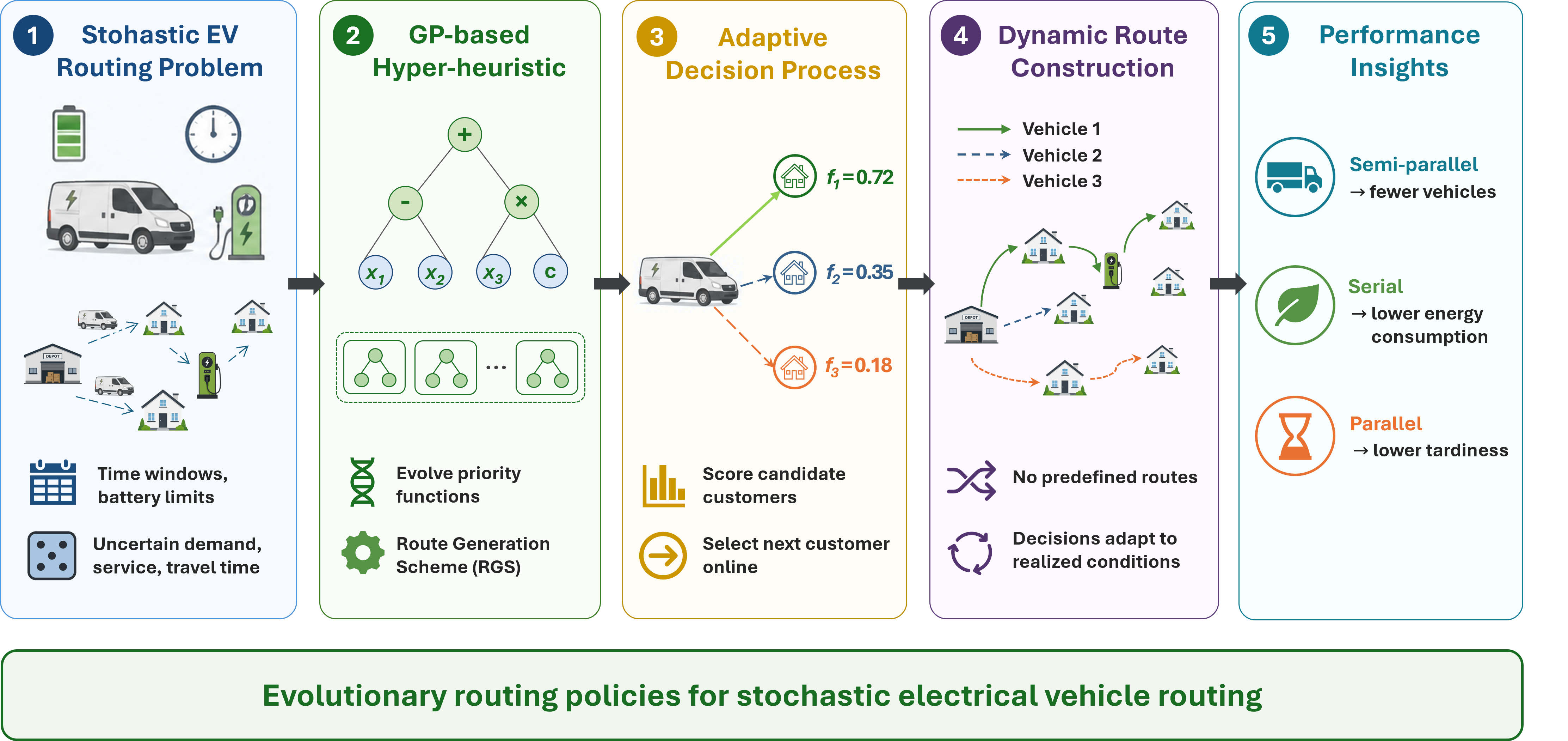
Figure 1 provides an overview of the proposed framework, including the offline evolution of priority functions and the online adaptive route construction process under stochastic realizations. The route construction process defined by the RGS is detailed in the following section, while the representation and learning of the priority function are described in Section 3.5.
3.4. Route Generation Scheme
RGS defines the mechanism by which vehicle routes are constructed. In this study, five variants are considered: the Serial, Semi-parallel, and Parallel schemes adopted from [20], along with two extensions proposed in this work, namely the Semi-parallel-B and Parallel-B variants.
3.4.1. Common Feasibility and Operational Rules
Energy feasibility is verified before each movement decision. A vehicle may proceed to a destination only if it has sufficient energy to (i) reach the destination and (ii) subsequently reach the nearest charging station, preventing infeasible states without access to recharging. If this condition is not satisfied, the vehicle first travels to a feasible charging station, recharges, and then continues its route. Charging stations are selected by minimizing the total energy required to travel from the current location to the station and from the station to the intended destination.
Under stochastic demand, the realized demand of a selected customer may exceed the vehicle’s remaining capacity. In such cases, the service attempt is aborted, the vehicle returns to the depot (via a charging station if necessary), and the route is finalized. The customer remains unserved and is reconsidered later. This mechanism ensures feasibility under stochastic realizations and is applied implicitly in all RGS variants, although omitted from Algorithm 1 for clarity.
Time windows are modeled as soft. Under stochastic variations in service time and travel speed, enforcing hard time windows would frequently lead to infeasible routes, introducing additional feasibility-repair mechanisms that are orthogonal to the focus of this study. Moreover, strict hard time windows are often unrealistic in practical settings, where delays can occur and are typically tolerated to some extent. Therefore, late arrivals are allowed but penalized in the objective function.
In the Semi-parallel and Parallel variants, denotes a capacity-based lower bound on the required number of vehicles, computed as
where is the set of customer nodes. This bound represents the minimum number of vehicles required to satisfy total nominal customer demand under cargo-capacity constraints.
3.4.2. Baseline RGS Variants
The Serial, Semi-parallel, and Parallel RGS variants adopted from [20] differ in how vehicles are activated and extended during route construction. In the Serial scheme, routes are constructed sequentially by activating one vehicle at a time. In contrast, the Semi-parallel and Parallel schemes extend multiple routes concurrently, initially activating vehicles. The Semi-parallel variant selects the earliest available vehicle for extension and may switch to sequential construction if all active vehicles complete their routes. The Parallel variant maintains continuous parallelism by immediately activating a new vehicle whenever one completes its route. All variants follow the same route construction logic: routes are incrementally extended by selecting an unserved customer, verifying capacity and energy feasibility, and either continuing the route or returning the vehicle to the depot. The differences between variants lie solely in vehicle initialization and selection policies.
3.4.3. Extended RGS with Candidate Set Selection
The proposed Semi-parallel-B and Parallel-B variants extend their respective base schemes by modifying the vehicle selection mechanism. Instead of selecting only the earliest available vehicle, the set of the K earliest available vehicles is considered, and the vehicle with the largest remaining capacity is chosen. In this study, K is set to 3, providing a small but diverse candidate set that allows capacity-aware selection while keeping the decision process local and computationally efficient. This modification improves robustness under stochastic demand by reducing the likelihood of premature capacity saturation and unnecessary route termination.
3.4.4. Unified RGS Framework
All variants described above can be expressed within a single unified route construction framework. The variants differ only in vehicle initialization, selection, and update rules, while the underlying route construction logic remains identical. This unified procedure is presented in Algorithm 1, with variant-specific rules summarized in Table 1.
| Algorithm 1 Unified RGS framework |
|
3.5. Genetic Programming for Evolving Priority Functions
While the RGS defines how routes are constructed, the quality of the routing policy depends on the rule used to select the next customer at each decision point. In this work, this rule is represented by a priority function (PF), which assigns a numerical score to each unserved customer, and the customer with the highest score is selected.
The PF is automatically evolved using Genetic Programming (GP), which constructs decision rules by combining problem-specific features through mathematical operators [21,45]. Each GP individual represents a candidate PF encoded as an expression tree, where terminal nodes correspond to features of the current system state and internal nodes represent mathematical operators.
During route construction, the expression tree is evaluated for each candidate customer. Since some features depend on stochastic quantities (e.g., travel times or arrival times), a single evaluation may be sensitive to random realizations. To mitigate this effect, each candidate is evaluated multiple times under independent stochastic samples. In this work, the evaluation is repeated five times, providing a small number of samples that stabilizes the selection while keeping the computational cost manageable. The most frequently preferred customer is then selected. In the case of ties, preference is given to the customer selected by the smaller GP expression tree. This sampling-based decision mechanism improves robustness while maintaining computational efficiency.
The GP procedure follows a standard generational evolutionary scheme, where a population of candidate PFs is iteratively improved through selection, crossover, and mutation. The initial population consists of expression trees generated using the full method [21], with a depth of five. During evolution, the tree depth is limited to , and individuals exceeding this limit are considered invalid and removed from the population. The evolutionary process runs for a fixed number of generations. The configuration largely follows standard GP settings, consistent with common practice [21] and with prior GP-based routing approaches [20]. The general workflow is shown in Algorithm 2, and the configuration parameters used in the experiments are summarized in Table 2. The implementation is based on the Jenetics1 evolutionary computation library (version 8.3.0).
| Algorithm 2 Descriptive evolutionary workflow in Jenetics |
|
3.5.1. Terminal and Function Nodes
The primitive set builds upon the terminals and functions proposed in [20], which are retained to preserve the original EVRPTW routing policy framework. To address the stochastic setting considered in this work, the terminal set is extended with stochastic descriptors (, , ) intended to capture expected variability in customer demand, travel time, and service time, as well as global-state and coordination descriptors (, , , ) intended to provide information about the remaining workload, available vehicle resources, and interactions between concurrently active vehicles. In addition, is included to provide information about the remaining time-window slack available for servicing a customer.
For objective-specific optimization, is introduced for the vehicle minimization objective to capture the minimum remaining capacity among active vehicles, while is introduced for tardiness minimization to capture the available temporal slack of the currently considered vehicle for customer i, computed as the difference between the customer due time and the estimated vehicle arrival time.
Due to the online nature of the stochastic setting, realized stochastic values are not available during customer selection. Consequently, all terminal nodes whose computation depends on stochastic quantities are evaluated using nominal parameter values. The complete set of terminal nodes is summarized in Table 3, while their relevance and usage patterns within evolved routing policies are further analyzed in Section 4.6.
The function nodes used in the GP representation are summarized in Table 4. The first row contains binary operators, and the second row contains unary operators. To ensure numerical stability during tree evaluation, the operators div, log, and sqr are implemented as safe functions. Specifically, div returns 0 when the denominator is close to zero, while log and sqr return 0 for non-positive arguments.
4. Results
4.1. Experimental Protocol
The experiments were conducted on a subset of Schneider’s benchmark instances [9] for the EVRPTW. In total, 48 instances were used, each consisting of 100 customers, 21 charging stations, and one depot. The focus on 100-customer instances was motivated by the stochastic setting considered in this work, as smaller instances tend to exhibit high variability and less stable routing behavior under random perturbations. According to the spatial distribution of customers, the instances are categorized into Clustered (C), Random (R), and Random-Clustered (RC) sets.
The dataset was split into mutually disjoint training and test sets. The training set contains 30 instances (10 C, 10 RC, and 10 R), while the test set contains the remaining 18 instances (6 C, 6 RC, and 6 R). The split preserves the balance across instance types and allocates a larger portion of instances to the test set to enable a more robust generalization evaluation. All results reported in this section are obtained on the test set, ensuring evaluation on previously unseen instances.
During training, each instance was evaluated twice per fitness computation in order to account for stochastic variability. All GP models were evolved under a fixed stochastic setting in which customer demand, service time, and vehicle speed follow a lognormal distribution with variability parameter . To account for both stochasticity and the randomness of GP initialization, the entire training procedure was repeated 10 times, resulting in 10 independently evolved PFs per optimization objective. This provides a representative sample of independently evolved PFs while keeping the computational cost manageable.
Each evolved PF was subsequently evaluated on a range of stochastic test scenarios. These scenarios systematically vary the distribution type and the level of variability for demand, service time, and vehicle speed. A test scenario is denoted as
where distribution specifies the probability distribution (DET for deterministic, LN for lognormal, and U for uniform), and , , and denote the variability parameters associated with customer demand, service time, and vehicle speed, respectively.
The deterministic scenario DET-0,0,0 corresponds to the standard EVRPTW without stochastic perturbations and serves as an internal baseline, enabling comparison with the original deterministic GP-RGS framework [20] under identical evaluation conditions and isolating the effect of incorporating stochastic information into the routing policy. This abbreviated notation is used consistently throughout the result tables.
The following evaluation scenarios were considered:
- DET-0,0,0
- LN-0.1,0,0, LN-0.2,0,0, LN-0.3,0,0
- LN-0,0.1,0, LN-0,0.2,0, LN-0,0.3,0
- LN-0,0,0.1, LN-0,0,0.2, LN-0,0,0.3
- LN-0.2,0.2,0, LN-0.2,0,0.2, LN-0,0.2,0.2
- LN-0.2,0.2,0.2, LN-0.3,0.3,0.3
- U-0.2,0.2,0.2, U-0.3,0.3,0.3
For each test scenario, every PF is evaluated on all 18 test instances (6 C, 6 RC, and 6 R). To account for stochastic variability, each instance is evaluated six times with independently sampled realizations of demand, service time, and travel time, resulting in 108 runs per scenario. For a given PF and scenario, the objective values are summed over all 108 runs, yielding a single score per PF. The reported results summarize the distribution of these scores across the 10 independently evolved PFs, both through descriptive statistics (min, avg, max) and through the full distributions shown in the violin plots. This evaluation procedure is applied consistently across all optimization objectives. The average online route-construction time on the considered 100-customer instances was approximately 10 ms per instance. To support reproducibility, the implementation used in this study is publicly available at: https://github.com/AlanDurdevic/stohastic-EVRP-GP.
4.2. Results for Vehicle Minimization Objective
Table 5 summarizes the results obtained when minimizing the number of vehicles. Figure 2 provides two complementary views of these results. The line plot (Figure 2) shows the average number of vehicles across all test scenarios and serves as the primary basis for comparing the methods. The results reveal a highly stable overall pattern. Semi-parallel and Semi-parallel-B consistently achieve the lowest average values, with only minor differences between them across scenarios. Serial consistently performs slightly worse than these two variants, but remains clearly better than the Parallel-based strategies. Among the latter, Parallel-B improves upon Parallel, although both remain substantially inferior to the Serial and Semi-parallel variants. This ordering is preserved across all scenarios, including the deterministic case (DET-0,0,0), indicating that stochasticity has little effect on the relative ranking of the RGS variants, although it does influence absolute performance levels.
The violin plots (Figure 2) complement this view by showing the full distribution of results across all runs. These distributions reinforce the separation between the methods: Semi-parallel and Semi-parallel-B are concentrated at the lowest values, Serial occupies a slightly higher but still compact range, while Parallel and Parallel-B are shifted to markedly higher values and exhibit much broader variability. This indicates that the Parallel-based strategies are not only worse on average, but also less stable under stochastic conditions. For completeness, detailed violin plots for each individual test scenario are provided in Appendix A.
The effect of the proposed B-modification varies across routing strategies. For the Parallel variant, Parallel-B consistently improves performance, leading to lower average values and reduced variability. This is reflected in both the average trends and the distributional view, where Parallel shows the highest values and widest spread, while Parallel-B shifts toward lower and more concentrated results. For the Semi-parallel strategy, the impact is less pronounced. Semi-parallel and Semi-parallel-B achieve very similar average results, with only minor differences across scenarios. However, the minimum values in Table 5 indicate that Semi-parallel-B more frequently attains the lowest minima, suggesting occasional improvements that are not consistently reflected in the average performance.
Regarding the influence of stochasticity, demand variability has the most pronounced effect on fleet size. As the variability parameter of customer demand increases, the average number of vehicles also increases across all methods, with the effect being particularly strong for the Parallel-based variants, which also exhibit increased variability. In contrast, variability in service time has little to no impact on fleet size, with both average values and distributions remaining largely unchanged across scenarios. Variability in vehicle speed has a moderate effect. While the overall ranking of methods remains unchanged, speed variability leads to a slight increase in dispersion and, in some cases, small shifts in average performance.
4.3. Results for Energy Consumption Minimization Objective
Table 6 summarizes the results obtained when minimizing energy consumption, while Figure 3 shows the corresponding average values across test scenarios and distributions. The average values (Figure 3) reveal a clear and stable separation for the best-performing method: the Serial variant consistently achieves the lowest energy consumption in all scenarios. Notably, this behavior is also observed in the deterministic scenario (DET-0,0,0), indicating that the superiority of the Serial strategy is not driven by stochastic effects, but rather reflects its inherently more energy-efficient routing structure. Beyond this, the ordering of the remaining methods is less consistent. Semi-parallel and Semi-parallel-B generally outperform the Parallel-based strategies, but their relative ranking varies across scenarios. Similarly, Parallel-B most often yields the highest energy consumption, although not in every instance. This indicates that, unlike the vehicle minimization objective, energy consumption is more sensitive to the interaction between routing strategy and stochastic variability, leading to scenario-dependent performance differences among the non-serial variants.
The influence of stochasticity depends on the source of uncertainty. Demand variability has only a minor effect, producing small changes in average values without altering the overall structure of the results. In contrast, variability in service time has a more structural impact: while its effect on average energy consumption is moderate, it can alter the relative performance of closely competing methods. In particular, the ordering between Semi-parallel and Semi-parallel-B is occasionally reversed under service-time variability. Variability in vehicle speed has a weaker influence, introducing modest shifts in average performance and increased dispersion without changing the overall ranking. Additional insight is provided by the minimum values reported in Table 6. Although the B-variants often exhibit worse average performance, they consistently achieve lower minimum values than their non-B counterparts, indicating that more energy-efficient solutions can occasionally be obtained.
The distributional view (Figure 3) supports these observations. Serial remains tightly concentrated at low values, indicating both strong performance and high stability. Semi-parallel and Semi-parallel-B exhibit a relatively compact spread, while the Parallel-based variants are shifted to higher values and display substantially greater dispersion. This is particularly evident for Parallel-B, which shows the widest spread and long upper tails, reflecting occasional highly inefficient solutions.
4.4. Results for Total Tardiness Minimization Objective
Table 7 summarizes the results for the tardiness objective, while Figure 4 presents the corresponding averages and distributions. In contrast to the energy objective, the performance hierarchy is clearly inverted. As shown in Figure 4, Parallel-based strategies achieve the lowest tardiness across all scenarios, with Parallel-B consistently achieving the lowest average values. The remaining methods exhibit more variability: Parallel generally performs well but is less stable, Semi-parallel variants occupy an intermediate range, while Serial performs worst by a substantial margin. This indicates that increased parallelism can be beneficial for handling time-window constraints, although its effectiveness depends on the specific routing strategy. This behavior is also observed in the deterministic scenario (DET-0,0,0), indicating that the advantage of Parallel-based strategies is not driven by stochastic effects but reflects their ability to better handle time-window constraints.
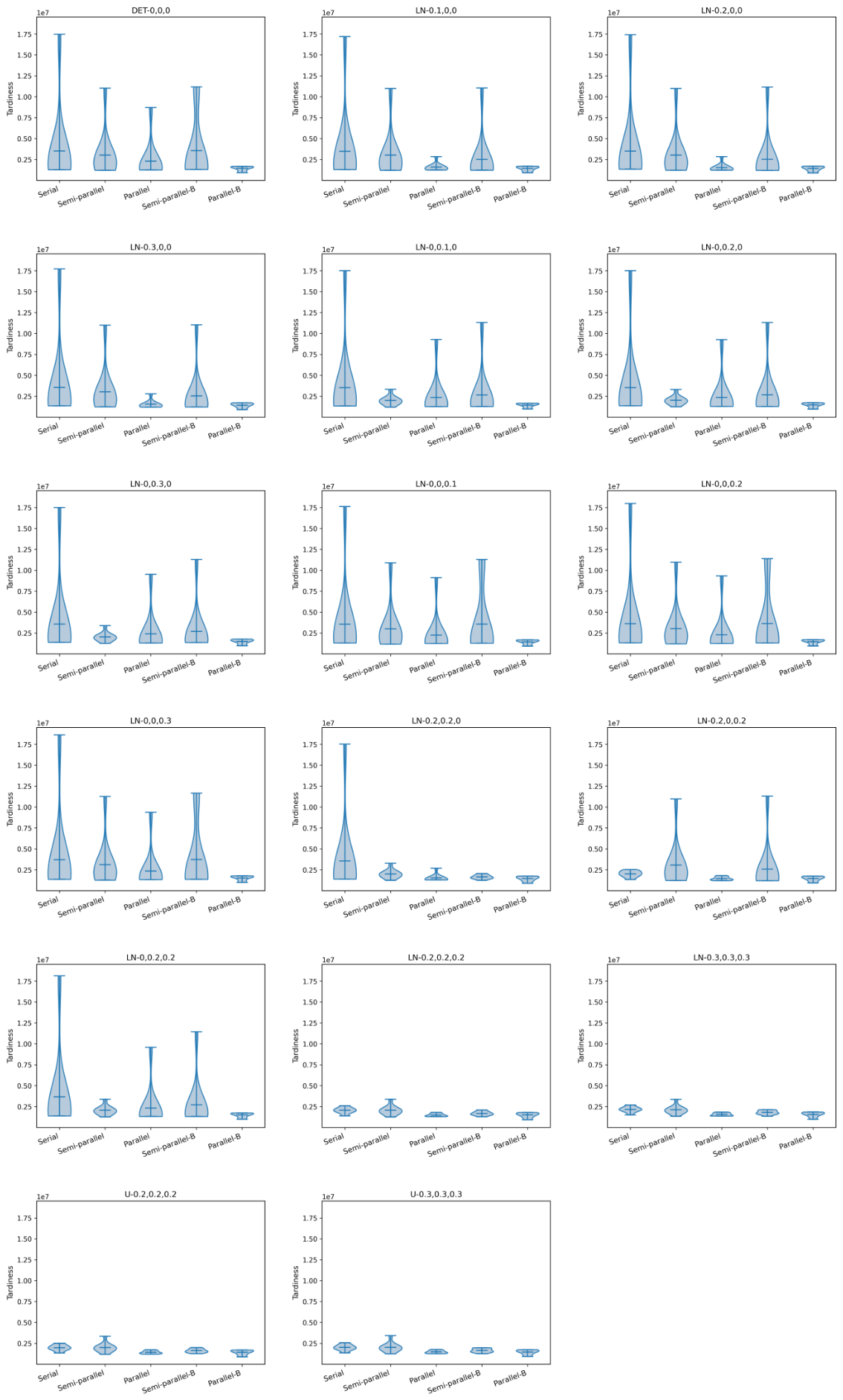
The distributional view (Figure 4) further supports these observations. Parallel-B achieves low average tardiness with relatively low variability, while Parallel exhibits comparable performance with somewhat higher dispersion. Parallel performs similarly, although with higher dispersion. In contrast, the Serial strategy shows both substantially higher average tardiness and a wide spread with long upper tails, indicating frequent occurrences of highly delayed solutions. Semi-parallel strategies occupy an intermediate position, with moderate dispersion and performance. Overall, these results suggest that higher degrees of parallelism tend to reduce tardiness and improve robustness, although differences between closely related variants are less pronounced.
The effect of the B-modification is most noticeable for the Parallel strategy, where Parallel-B generally achieves lower average tardiness and reduced variability. For the Semi-parallel strategy, the effect is less consistent, with Semi-parallel and Semi-parallel-B exhibiting similar performance across scenarios.
The influence of stochasticity does not follow a simple or monotonic pattern. Variations in individual factors often have limited or inconsistent effects on their own, while combinations of stochastic elements lead to abrupt changes in performance. In particular, changes in demand alone have little impact on tardiness, whereas variability in service time and vehicle speed can trigger sharp increases for certain strategies, most notably the Parallel variant. However, these effects are not cumulative in a predictable way: in scenarios where all three sources of uncertainty are present at moderate levels, the methods often stabilize and even show slight improvements in average performance.
4.5. Pairwise Comparison of Routing Strategies
While the previous analysis focuses on aggregated performance through averages and distributions, this section examines the consistency of pairwise differences between routing strategies across identical problem realizations. By comparing methods on a per-instance and per-run basis, the analysis isolates structural differences in decision behavior that may be obscured by aggregation.
Since all methods are evaluated on the same instances and stochastic realizations, observations are paired. Accordingly, statistical comparisons are performed using the Friedman test followed by pairwise Wilcoxon signed-rank tests with Holm correction. The Friedman test confirms the presence of statistically significant differences among routing strategies for all objectives (vehicles: , energy: , tardiness: ; all ), justifying subsequent pairwise analysis.
The results of the pairwise comparisons are summarized in Table 8. Rows and columns correspond to routing variants, and each cell reports the outcome of the Wilcoxon test with Holm correction. A checkmark () indicates a statistically significant difference (), while exact p-values are shown only for non-significant comparisons. For completeness, the median difference (row−column) is also provided; negative values indicate that the row method tends to achieve lower objective values than the column method.
For the vehicle objective, all pairwise differences are statistically significant. However, several comparisons exhibit zero median difference, indicating that the observed differences, although highly consistent across realizations, are practically small. This highlights that statistical significance in this setting primarily reflects consistency rather than effect magnitude.
For the energy objective, all pairwise differences are also statistically significant, reflecting a clear and consistent ordering of the methods. In this case, statistical significance aligns closely with practical relevance, as the observed median differences are substantial and consistent with the separation already visible in the aggregated results. This confirms that the dominance of the Serial strategy and the inferior performance of Parallel-based variants are not only evident on average, but persist across individual realizations.
For the tardiness objective, the results exhibit a different pattern. Most pairwise differences are statistically significant; however, the comparison between Parallel and Parallel-B is not significant (), indicating that these two strategies achieve comparable performance when evaluated on identical realizations. This contrasts with the distributional analysis, where differences in variability are apparent, and suggests that the distinction between these methods is driven more by dispersion and extreme outcomes than by consistent differences in central tendency. Overall, these findings reinforce that the effect of parallelism depends strongly on the objective, and that paired comparisons provide additional insight into the consistency of method behavior beyond aggregated performance measures.
4.6. Analysis of Terminal Node Usage
To gain insight into the decision mechanisms learned by the GP-based routing policies, we analyze terminal node usage across routing strategies and objectives. Specifically, we examine (i) the relative frequency of terminal nodes within evolved policies, grouped by routing strategy (RGS), and (ii) the association between terminal usage and objective values. Terminal frequencies are visualized using heatmaps (Figure 5), enabling identification of dominant features and structural differences between strategies. To assess functional relevance, we compute Spearman rank correlations between terminal usage and objective values (Figure 6). Only correlations with are reported, with stronger signals () highlighted, in order to retain consistent trends while accounting for the limited sample size per configuration.
For the vehicle minimization objective (Figure 5), Semi-parallel and Semi-parallel-B strategies are dominated by and , each accounting for nearly 50% of node usage. Parallel variants rely on the same features but exhibit a more distributed pattern, while the Serial strategy shows the most dispersed usage without a clearly dominant feature.
The correlation analysis (Figure 6) is consistent with the observed usage patterns. The feature exhibits a consistent negative correlation with the number of vehicles across semi-parallel and parallel strategies, indicating that prioritizing demand is associated with improved performance. In contrast, despite its high frequency, shows weak correlation with the objective, suggesting a supporting rather than driving role. The Serial strategy follows a different pattern, with stronger correlations for timing- and state-related features (e.g., , ), while demand-related signals remain less influential.
The terminal node distribution for the energy minimization objective (Figure 5) is dominated by across all strategies, particularly in semi-parallel variants. Beyond this common pattern, strategies differ in how additional features are used. The Serial strategy relies on a combination of energy-, demand-, and routing-related features, including , , and , all of which appear with notable frequency alongside . Semi-parallel variants remain strongly concentrated on , with relatively limited use of other terminals. In contrast, the Parallel strategy exhibits a more distributed pattern across multiple terminals, including additional energy-related and stochastic descriptors such as , , and . The Parallel-B variant follows a more constrained pattern, relying on fewer additional features compared to Parallel.
A clear pattern emerges in the correlation results (Figure 6): each routing strategy is primarily associated with a single dominant feature. The Serial strategy shows a strong negative correlation with , while semi-parallel variants exhibit a positive correlation with the demand-related feature . In contrast, the Parallel strategy shows significant correlations for multiple features, most notably , indicating a broader set of influencing features. The Parallel-B variant exhibits a negative correlation with , but without additional strongly correlated features.
For the tardiness minimization objective (Figure 5), remains the most frequently used feature across all strategies, but is accompanied by a broader use of additional terminals, particularly in Parallel and Parallel-B. These strategies show increased utilization of customer- and timing-related features (e.g., , , , , ), as well as system-level descriptors such as , indicating a more diverse decision basis combining feasibility, timing, and urgency information. In contrast, the Serial strategy distributes importance across multiple features without a clearly dominant signal, while the Semi-parallel strategy remains largely centered on with limited contribution from timing- or urgency-related features.
The correlation results (Figure 6) show that , one of the newly introduced system-level descriptors, exhibits the strongest positive correlation with the objective in the Parallel strategy. In contrast, , although the most frequently used terminal, does not show consistently strong correlation. In Parallel-B, multiple features (including , , and ) exhibit significant correlations, indicating a more distributed pattern. Other strategies are typically associated with a single dominant correlated feature (e.g., or in Serial, in Semi-parallel), although these signals are generally weaker or less consistent.
4.7. Comparison with Greedy Baselines
To provide additional context regarding the effectiveness of the proposed GP-based routing policies, we compare them against several simple constructive heuristics commonly used in routing settings:
- Nearest Neighbor (NN): selects the geographically closest feasible customer.
- Minimum Travel Energy (MTE): selects the customer with the lowest feasible travel-energy cost.
- Minimum Slack (MS): selects the customer with the smallest remaining time-window slack.
- Earliest Due Time (EDT): selects the customer with the earliest due time.
All greedy heuristics were implemented within the same route-construction framework as the proposed approach, replacing the GP-evolved priority function with the corresponding hand-designed rule. To isolate the effect of customer-selection policies, all greedy baselines use the Serial RGS variant. Since each heuristic corresponds to a single deterministic policy, only aggregated objective values are reported. The results are shown in Figure 7.
The nearest-neighbor heuristic remains competitive for fleet-size minimization in deterministic and low-variability scenarios, occasionally achieving slightly lower values than the GP-based Semi-parallel policy. However, its performance deteriorates more rapidly as demand variability increases, while the GP-based approaches remain more stable across stochastic settings.
For the energy objective, the GP-based Serial policy consistently achieves the lowest consumption across all tested scenarios. Although the minimum-travel-energy heuristic remains competitive, the remaining hand-designed heuristics perform substantially worse.
The largest performance differences are observed for tardiness, where the GP-based Parallel-B strategy consistently outperforms all greedy baselines, suggesting that the evolved policies better balance routing, scheduling, and charging decisions under stochastic operating conditions.
5. Discussion
5.1. Vehicle Minimization
The results largely follow the main conclusions reported in [20], where Serial and Semi-parallel strategies outperform the Parallel approach in terms of fleet size. However, under stochastic conditions the balance shifts more clearly toward limited parallelism, with Semi-parallel and Semi-parallel-B consistently achieving better results than Serial across all scenarios. Fully sequential construction delays the activation of additional vehicles, which becomes problematic when stochastic realizations disrupt routes, while fully parallel construction fragments the solution too early and reduces capacity utilization efficiency. Semi-parallel approaches maintain enough structure to avoid fragmentation while still reacting to emerging constraints. The B-modification further reinforces this behavior by prioritizing vehicles with larger remaining capacity and reducing the risk of premature capacity saturation. Among the considered stochastic factors, demand variability has the strongest influence on fleet size, directly affecting capacity feasibility and often forcing the use of additional vehicles, whereas service-time variability has relatively limited effect and travel-time variability mainly increases dispersion without changing the relative ordering of routing strategies. Although the absolute differences between methods remain relatively small, the statistical analysis confirms that these patterns are highly consistent across stochastic scenarios.
The node analysis further supports these observations. Vehicle minimization is primarily associated with the combined use of and , particularly in the Semi-parallel and Semi-parallel-B variants. The negative correlation of with the objective indicates that prioritizing demand contributes to reducing fleet size, while the high usage but weak correlation of suggests a supporting feasibility-related role. In contrast, the Serial strategy relies more heavily on timing- and state-related features and exhibits weaker demand-related signals, consistent with its less effective handling of capacity utilization. Stochastic descriptors show limited influence in both usage and correlation analyses, suggesting that vehicle minimization is driven primarily by stable structural routing behavior rather than explicit modeling of variability.
5.2. Energy Minimization
For the energy minimization objective, the relative behavior of routing strategies changes substantially. Consistent with [20], the Serial strategy achieves the best overall performance. Unlike vehicle minimization, where limited parallelism is beneficial, energy minimization favors sequential route construction, which produces geographically compact routes. Because of this structure, the Serial strategy remains comparatively stable even when stochastic travel-time variability increases. In contrast, Parallel-based strategies activate multiple routes early, producing longer, less coherent routes with higher energy consumption. Under stronger stochastic variability, this leads to dispersed and occasional highly inefficient solutions, particularly for Parallel-B, where prioritizing vehicles with larger remaining capacity further reduces route compactness. Semi-parallel variants maintain a more balanced trade-off and therefore remain considerably more stable across stochastic scenarios.
The node analysis further clarifies these differences. In the Serial strategy, energy minimization is associated with a strong negative correlation of , indicating that decisions are guided by a feature directly related to energy cost. In contrast, semi-parallel strategies mostly use node but their correlation is driven by demand-related features such as , suggesting a weaker alignment between dominant signals and the objective. Parallel variants do not exhibit a clearly dominant energy-related decision signal, consistent with their weaker performance for the energy objective.
5.3. Tardiness Minimization
Unlike energy minimization, which favors sequential route construction, tardiness minimization benefits from early and distributed route activation. As also observed in [20], Parallel-based strategies achieve the best overall performance by reducing the accumulation of delays within individual routes. In contrast, the Serial strategy delays vehicle activation, making recovery from stochastic disruptions more difficult. In highly parallel settings, the B-modification further improves average tardiness and solution stability by prioritizing vehicles with larger remaining capacity among the earliest available candidates. However, the lack of statistically significant differences between Parallel and Parallel-B suggests that the primary advantage lies in the degree of parallelism itself rather than in the specific vehicle-selection variant. Unlike the energy objective, the influence of stochasticity on tardiness is less structured and does not follow simple monotonic trends. Individual sources of variability often produce limited effects, while specific combinations can trigger abrupt performance changes and occasional spikes, indicating stronger interactions between stochastic components.
The node analysis suggests that each routing strategy tends to rely on a small number of dominant signals. In the Parallel strategy, the strongest correlation is observed for the system-level descriptor , suggesting that global information regarding the number of remaining unserved customers becomes particularly relevant in highly parallel routing settings, where coordination between concurrently active vehicles plays a larger role. Parallel-B exhibits a more distributed set of significant correlations, including , , and , while other strategies are typically associated with only one dominant correlated feature.
5.4. Overall Observations
Taken together, the results indicate that no single routing strategy is universally optimal across objectives. Instead, the effectiveness of route construction depends strongly on the interaction between the optimization objective, the degree of parallelism, and the underlying stochastic conditions. Vehicle minimization benefits from limited parallelism and balanced capacity utilization, energy minimization favors sequential and spatially coherent routing, while tardiness minimization benefits from early workload distribution across multiple vehicles. Across all objectives, stochasticity primarily amplifies these structural differences rather than fundamentally altering the relative behavior of routing strategies. The node analysis further suggests that effective routing policies emerge through different combinations of dominant decision signals depending on the objective and route-construction scheme.
6. Conclusions
This paper presented an extension of a GP-based RGS framework to the stochastic electric vehicle routing problem with time windows. The proposed approach incorporates uncertainty in customer demand, service time, and travel time through controlled stochastic perturbations, while extending the GP priority function with stochastic and global-state descriptors. In addition, two new route-generation variants, Semi-parallel-B and Parallel-B, were introduced to improve capacity-aware vehicle selection under uncertainty.
The results show that routing strategy performance depends strongly on the optimization objective. Semi-parallel strategies achieved the best fleet-size performance by balancing capacity utilization and routing flexibility, while the Serial strategy consistently achieved the lowest energy consumption by preserving spatial coherence and compact routes. In contrast, Parallel-based strategies achieved the best tardiness performance by distributing workload earlier across multiple vehicles and reducing delay accumulation. Across objectives, stochasticity primarily amplified the structural differences between routing strategies rather than altering their relative behavior. The node analysis further showed that effective routing policies rely on a relatively small number of objective-relevant decision signals, with the newly introduced system-level descriptor exhibiting a particularly strong association with tardiness minimization in highly parallel routing settings.
Additional experiments with hand-designed constructive heuristics further showed that the proposed GP-based policies remain competitive across stochastic scenarios and substantially outperform simple greedy baselines for the tardiness objective. Overall, the results support the suitability of lightweight evolutionary hyper-heuristics for constructing adaptive routing policies in stochastic EVRPTW environments.
The present study focuses on policy-based constructive heuristics under controlled stochastic settings rather than on large-scale stochastic optimization approaches. While comparisons with stochastic programming or reinforcement learning methods would provide additional perspective, such approaches operate under substantially different modeling and computational assumptions. Furthermore, uncertainty was modeled using parametric distributions in a static stochastic setting, enabling systematic and reproducible evaluation but not fully capturing the complexity of real-world logistics systems.
In addition, charging-station locations were treated as fixed exogenous components of the benchmark instances, and the robustness of the proposed routing policies under varying charging-network configurations was not investigated. Future work will therefore focus on extending the proposed framework to dynamic and real-time routing environments, incorporating richer data-driven uncertainty models, evaluating the approach on real-world operational datasets, and analyzing routing-policy behavior under alternative charging-infrastructure layouts and configurations.
Author Contributions
Conceptualization, N.F. and M.Đ.; methodology, A.Đ. and N.F.; software, A.Đ.; validation, A.Đ. and N.F.; formal analysis, A.Đ. and N.F; investigation, A.Đ.; resources, M.Đ.; writing—original draft preparation, A.Đ. and N.F.; writing—review and editing, A.Đ. and N.F., and M.Đ.; visualization, A.Đ.; supervision, N.F. and M.Đ.; project administration, M.Đ.; funding acquisition, M.Đ. All authors have read and agreed to the published version of the manuscript.
Funding
This work has been supported by the European Union - NextGenerationEU under the grant NPOO.C3.2.R2-I1.06.0110.
Data Availability Statement
No new data were created or analyzed in this study. Data sharing is not applicable to this article.
Conflicts of Interest
The authors declare no conflicts of interest. The funders had no role in the design of the study; in the collection, analyses, or interpretation of data; in the writing of the manuscript; or in the decision to publish the results.
Abbreviations
The following abbreviations are used in this manuscript:
| VRP | Vehicle Routing Problem |
| VRPTW | Vehicle Routing Problem with Time Windows |
| EVRP | Electric Vehicle Routing Problem |
| EVRPTW | Electric Vehicle Routing Problem with Time Windows |
| RGS | Route Generation Scheme |
| PF | Priority Function |
| GP | Genetic Programming |
| ALNS | Adaptive Large Neighborhood Search |
| ILS | Iterated Local Search |
| VNS | Variable Neighborhood Search |
Appendix A. Scenario-Wise Distribution of Objective Values
This appendix provides a more detailed view of the experimental results through scenario-wise violin plots for all three optimization objectives. Unlike the aggregated plots presented in the main text, these figures show the distribution of results separately for each test scenario and for each route generation scheme. In this way, they provide additional insight into the variability, spread, and shape of the obtained outcomes under different stochastic settings.
Figure A1.
Scenario-wise violin plots for the vehicle minimization objective. Each subplot corresponds to one experimental scenario and shows the distribution of the number of vehicles obtained for the five route generation schemes over all runs.
Figure A1.
Scenario-wise violin plots for the vehicle minimization objective. Each subplot corresponds to one experimental scenario and shows the distribution of the number of vehicles obtained for the five route generation schemes over all runs.
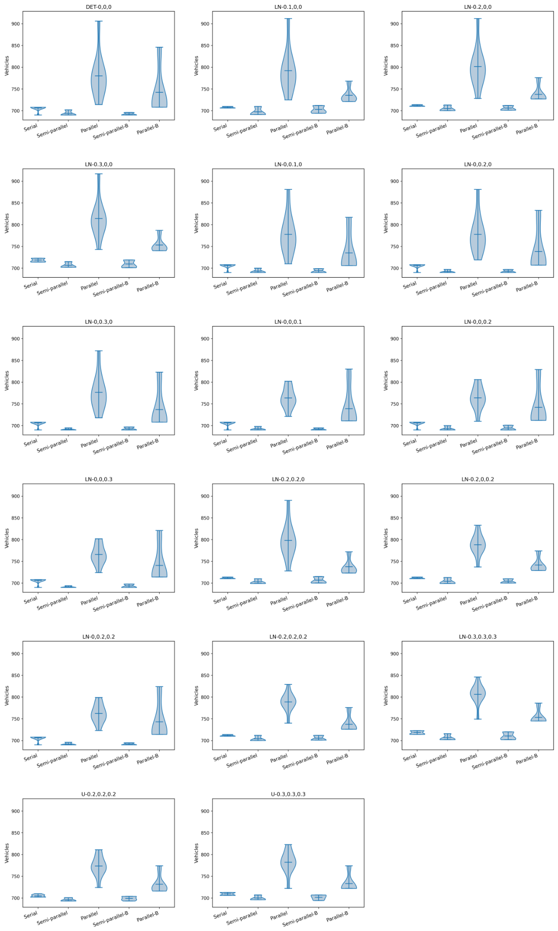
Figure A2.
Scenario-wise violin plots for the energy minimization objective. Each subplot corresponds to one experimental scenario and shows the distribution of energy consumption obtained for the five route generation schemes over all runs.
Figure A2.
Scenario-wise violin plots for the energy minimization objective. Each subplot corresponds to one experimental scenario and shows the distribution of energy consumption obtained for the five route generation schemes over all runs.
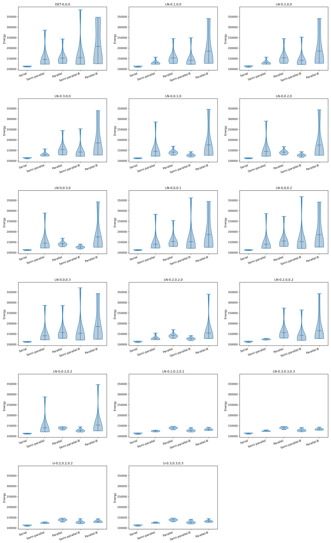
Figure A3.
Scenario-wise violin plots for the tardiness minimization objective. Each subplot corresponds to one experimental scenario and shows the distribution of tardiness values obtained for the five route generation schemes over all runs.
Figure A3.
Scenario-wise violin plots for the tardiness minimization objective. Each subplot corresponds to one experimental scenario and shows the distribution of tardiness values obtained for the five route generation schemes over all runs.
Appendix B. Convergence Analysis
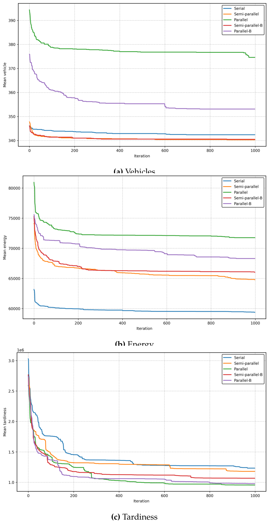
This appendix provides additional details on the convergence behavior of the GP-based approach across different routing strategies and optimization objectives. The results illustrate the evolution of objective values over generations, allowing comparison of convergence speed and stability under different stochastic settings. The curves show the average across all experiments for each method.
Figure A4.
Mean objective value per iteration for the five algorithm variants: Serial, Semi-parallel, Parallel, Semi-parallel-B, and Parallel-B.
Figure A4.
Mean objective value per iteration for the five algorithm variants: Serial, Semi-parallel, Parallel, Semi-parallel-B, and Parallel-B.
References
- Braekers, K.; Ramaekers, K.; Van Nieuwenhuyse, I. The vehicle routing problem: State of the art classification and review. Comput. Ind. Eng. 2016, 99, 300–313. [Google Scholar] [CrossRef]
- Zhang, S.; Chen, M.; Zhang, W.; Zhuang, X. Fuzzy optimization model for electric vehicle routing problem with time windows and recharging stations. Expert Syst. With Appl. 2020, 145, 113123. [Google Scholar] [CrossRef]
- Feng, B.; Wei, L. An improved multi-directional local search algorithm for vehicle routing problem with time windows and route balance. Appl. Intell. 2023. [Google Scholar] [CrossRef]
- Jonge, D.; Bistaffa, F.; Levy, J. Multi-Objective Vehicle Routing with Automated Negotiation. Appl. Intell. 2022, 52. [Google Scholar] [CrossRef]
- Moghdani, R.; Salimifard, K.; Demir, E.; Benyettou, A. The green vehicle routing problem: A systematic literature review. J. Clean. Prod. 2021, 279, 123691. [Google Scholar] [CrossRef]
- Kucukoglu, I.; Dewil, R.; Cattrysse, D. The electric vehicle routing problem and its variations: A literature review. Comput. Ind. Eng. 2021, 161, 107650. [Google Scholar] [CrossRef]
- Hien, V.Q.; Dao, T.C.; Binh, H.T.T. A greedy search based evolutionary algorithm for electric vehicle routing problem. Appl. Intell. 2023, 53, 2908–2922. [Google Scholar] [CrossRef]
- Schiffer, M.; Klein, P.S.; Laporte, G.; Walther, G. Integrated planning for electric commercial vehicle fleets: A case study for retail mid-haul logistics networks. Eur. J. Oper. Res. 2021, 291, 944–960. [Google Scholar] [CrossRef]
- Schneider, M.; Stenger, A.; Goeke, D. The Electric Vehicle-Routing Problem with Time Windows and Recharging Stations. Transp. Sci. 2014, 48, 500–520. [Google Scholar] [CrossRef]
- Solomon, M.M. Algorithms for the Vehicle Routing and Scheduling Problems with Time Window Constraints. Oper. Res. 1987, 35, 254–265. [Google Scholar] [CrossRef]
- Keskin, M.; Çatay, B. Partial recharge strategies for the electric vehicle routing problem with time windows. Transp. Res. Part C Emerg. Technol. 2016, 65, 111–127. [Google Scholar] [CrossRef]
- Montoya, A.; Guéret, C.; Mendoza, J.E.; Villegas, J.G. The electric vehicle routing problem with nonlinear charging function. Transportation Res. Part B Methodol.> 2017;Green. Urban Transp. 103, 87–110. [CrossRef]
- Bruglieri, M.; Pezzella, F.; Pisacane, O.; Suraci, S. A Variable Neighborhood Search Branching for the Electric Vehicle Routing Problem with Time Windows. Electronic Notes in Discrete Mathematics The 3rd International Conference on Variable Neighborhood Search (VNS’14), 2015; 47, pp. 221–228. [Google Scholar] [CrossRef]
- Gendreau, M.; Laporte, G.; Séguin, R. Stochastic vehicle routing. Eur. J. Oper. Res. 1996, 88, 3–12. [Google Scholar] [CrossRef]
- Cordeau, J.F.; Laporte, G.; Savelsbergh, M.; Vigo, D. Vehicle Routing. 2007, Vol. 14, 195–224. [Google Scholar]
- Keskin, M.; Çatay, B.; Laporte, G. A simulation-based heuristic for the electric vehicle routing problem with time windows and stochastic waiting times at recharging stations. Comput. Oper. Res. 2021, 125, 105060. [Google Scholar] [CrossRef]
- Ge, X.; Zhu, Z.; Jin, Y. Electric Vehicle Routing Problems with Stochastic Demands and Dynamic Remedial Measures. Math. Probl. Eng. 2020, 2020, 8795284. [Google Scholar] [CrossRef]
- Basso, R.; Kulcsár, B.; Sanchez-Diaz, I.; Qu, X. Dynamic stochastic electric vehicle routing with safe reinforcement learning. Transp. Res. Part E Logist. Transp. Rev. 2022, 157, 102496. [Google Scholar] [CrossRef]
- Aghalari, A.; Salamah, D.; Kabli, M.; Marufuzzaman, M. A two-stage stochastic location–routing problem for electric vehicles fast charging. Comput. Oper. Res. 2023, 158, 106286. [Google Scholar] [CrossRef]
- Gil-Gala, F.J.; Đurasević, M.; Jakobović, D. Evolving routing policies for electric vehicles by means of genetic programming. Appl. Intell. 2024, 54, 12391–12419. [Google Scholar] [CrossRef]
- Poli, R.; Langdon, W.; Mcphee, N. A Field Guide To Genet. Program. 2008.
- Hiermann, G.; Puchinger, J.; Ropke, S.; Hartl, R.F. The Electric Fleet Size and Mix Vehicle Routing Problem with Time Windows and Recharging Stations. Eur. J. Oper. Res. 2016, 252, 995–1018. [Google Scholar] [CrossRef]
- Keskin, M.; Çatay, B. A matheuristic method for the electric vehicle routing problem with time windows and fast chargers. Comput. Oper. Res. 2018, 100, 172–188. [Google Scholar] [CrossRef]
- Jie, W.; Yang, J.; Zhang, M.; Huang, Y. The two-echelon capacitated electric vehicle routing problem with battery swapping stations: Formulation and efficient methodology. Eur. J. Oper. Res. 2019, 272, 879–904. [Google Scholar] [CrossRef]
- Taş, D. Electric vehicle routing with flexible time windows: a column generation solution approach. Transp. Lett. 2021, 13, 97–103. [Google Scholar] [CrossRef]
- Duman, E.N.; Taş, D.; Çatay, B. Branch-and-price-and-cut methods for the electric vehicle routing problem with time windows. Int. J. Prod. Res. 2022, 60, 5332–5353. [Google Scholar] [CrossRef]
- Lam, E.; Desaulniers, G.; Stuckey, P.J. Branch-and-cut-and-price for the Electric Vehicle Routing Problem with Time Windows, Piecewise-Linear Recharging and Capacitated Recharging Stations. Comput. Oper. Res. 2022, 145, 105870. [Google Scholar] [CrossRef]
- Liu, Z.; Zuo, X.; Zhou, M.; Guan, W.; Al-Turki, Y. Electric Vehicle Routing Problem With Variable Vehicle Speed and Soft Time Windows for Perishable Product Delivery. IEEE Trans. Intell. Transp. Syst. 2023, 24, 6178–6190. [Google Scholar] [CrossRef]
- Lera-Romero, G.; Miranda Bront, J.J.; Soulignac, F.J. A branch-cut-and-price algorithm for the time-dependent electric vehicle routing problem with time windows. Eur. J. Oper. Res. 2024, 312, 978–995. [Google Scholar] [CrossRef]
- DROR, M.; LAPORTE, G.; TRUDEAU, P. Vehicle Routing with Stochastic Demands: Properties and Solution Frameworks. Transp. Sci. 1989, 23, 166–176. [Google Scholar] [CrossRef]
- LAPORTE, G.; LOUVEAUX, F.; MERCURE, H. The Vehicle Routing Problem with Stochastic Travel Times. Transp. Sci. 1992, 26, 161–170. [Google Scholar] [CrossRef]
- Kenyon, A.S.; Morton, D.P. Stochastic Vehicle Routing with Random Travel Times. Transp. Sci. 2003, 37, 69–82. [Google Scholar] [CrossRef]
- Laporte, G.; Louveaux, F.V.; van Hamme, L. An Integer L-Shaped Algorithm for the Capacitated Vehicle Routing Problem with Stochastic Demands. Oper. Res. 2002, 50, 415–423. [Google Scholar] [CrossRef]
- Christiansen, C.H.; Lysgaard, J. A branch-and-price algorithm for the capacitated vehicle routing problem with stochastic demands. Oper. Res. Lett. 2007, 35, 773–781. [Google Scholar] [CrossRef]
- Secomandi, N. Comparing neuro-dynamic programming algorithms for the vehicle routing problem with stochastic demands. Comput. Oper. Res. 2000, 27, 1201–1225. [Google Scholar] [CrossRef]
- Spinelli, A.; Bezzi, D.; Jabali, O.; Maggioni, F. A stochastic electric vehicle routing problem under uncertain energy consumption. Transp. Res. Part C Emerg. Technol. 2026, 183, 105480. [Google Scholar] [CrossRef]
- Wu, Y.; Song, W.; Cao, Z.; Zhang, J.; Lim, A. Learning Improvement Heuristics for Solving Routing Problems. IEEE Trans. Neural Netw. Learn. Syst. 2022, 33, 5057–5069. [Google Scholar] [CrossRef] [PubMed]
- Branke, J.; Nguyen, S.; Pickardt, C.W.; Zhang, M. Automated Design of Production Scheduling Heuristics: A Review. IEEE Trans. Evol. Comput. 2016, 20, 110–124. [Google Scholar] [CrossRef]
- Zhang, F.; Mei, Y.; Nguyen, S.; Zhang, M. Survey on Genetic Programming and Machine Learning Techniques for Heuristic Design in Job Shop Scheduling. IEEE Trans. Evol. Comput. 2024, 28, 147–167. [Google Scholar] [CrossRef]
- MacLachlan, J.; Mei, Y.; Branke, J.; Zhang, M. Genetic Programming Hyper-Heuristics with Vehicle Collaboration for Uncertain Capacitated Arc Routing Problems. Evol. Comput. 2020, 28, 563–593. [Google Scholar] [CrossRef]
- Gil-Gala, F.J.; Durasević, M.; Sierra, M.R.; Varela, R. Evolving ensembles of heuristics for the travelling salesman problem. Nat. Comput. 2023, 22, 671–684. [Google Scholar] [CrossRef]
- Jacobsen-Grocott, J.; Mei, Y.; Chen, G.; Zhang, M. Evolving heuristics for Dynamic Vehicle Routing with Time Windows using genetic programming. In Proceedings of the 2017 IEEE Congress on Evolutionary Computation (CEC), 2017; pp. 1948–1955. [Google Scholar] [CrossRef]
- Jakobović, D.; Đurasević, M.; Brkić, K.; Fosin, J.; Carić, T.; Davidović, D. Evolving Dispatching Rules for Dynamic Vehicle Routing with Genetic Programming. Algorithms 2023, 16, 285. [Google Scholar] [CrossRef]
- Gil-Gala, F.J.; Đurasević, M.; Jakobović, D.; Varela, R. Genetic programming with surrogate evaluation for the electric vehicle routing problem. Swarm Evol. Comput. 2025, 96, 101969. [Google Scholar] [CrossRef]
- Burke, E.K.; Hyde, M.R.; Kendall, G.; Woodward, J. Automating the Packing Heuristic Design Process with Genetic Programming. Evol. Comput. 2012, 20, 63–89. [Google Scholar] [CrossRef]
Figure 1.
Overview of the proposed GP-based routing framework for stochastic EV routing. Offline training evolves priority functions represented as GP trees, while online execution adaptively constructs routes under stochastic realizations.
Figure 1.
Overview of the proposed GP-based routing framework for stochastic EV routing. Offline training evolves priority functions represented as GP trees, while online execution adaptively constructs routes under stochastic realizations.
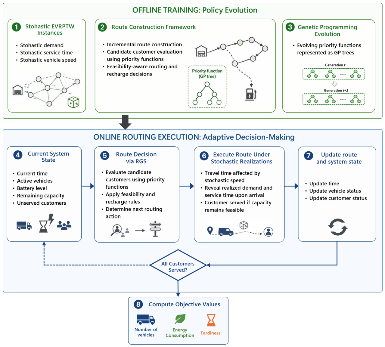
Figure 2.
Results for the vehicle minimization objective. (a) Average number of vehicles for each RGS variant across all test scenarios. Scenario labels follow the format distribution-, where denote variability in demand, service time, and vehicle speed, respectively. (b) Violin plots showing the distribution of vehicle counts for each RGS variant across all scenarios and runs.
Figure 2.
Results for the vehicle minimization objective. (a) Average number of vehicles for each RGS variant across all test scenarios. Scenario labels follow the format distribution-, where denote variability in demand, service time, and vehicle speed, respectively. (b) Violin plots showing the distribution of vehicle counts for each RGS variant across all scenarios and runs.
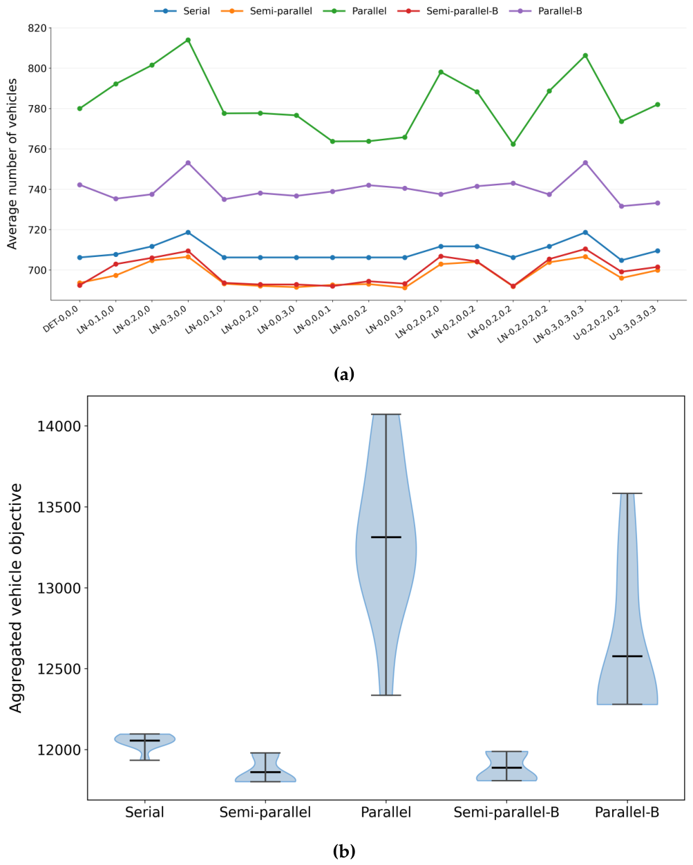
Figure 3.
Results for the energy minimization objective. (a) Average energy consumption for each RGS variant across all test scenarios. Scenario labels follow the format distribution-, where denote variability in demand, service time, and vehicle speed, respectively. (b) Violin plots showing the distribution of energy consumption for each RGS variant across all scenarios and runs.
Figure 3.
Results for the energy minimization objective. (a) Average energy consumption for each RGS variant across all test scenarios. Scenario labels follow the format distribution-, where denote variability in demand, service time, and vehicle speed, respectively. (b) Violin plots showing the distribution of energy consumption for each RGS variant across all scenarios and runs.
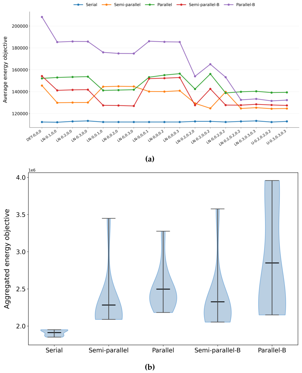
Figure 4.
Results for the tardiness minimization objective. (a) Average tardiness for each RGS variant across all test scenarios. Scenario labels follow the format distribution-, where denote variability in demand, service time, and vehicle speed, respectively. (b) Violin plots showing the distribution of tardiness for each RGS variant across all scenarios and runs.
Figure 4.
Results for the tardiness minimization objective. (a) Average tardiness for each RGS variant across all test scenarios. Scenario labels follow the format distribution-, where denote variability in demand, service time, and vehicle speed, respectively. (b) Violin plots showing the distribution of tardiness for each RGS variant across all scenarios and runs.
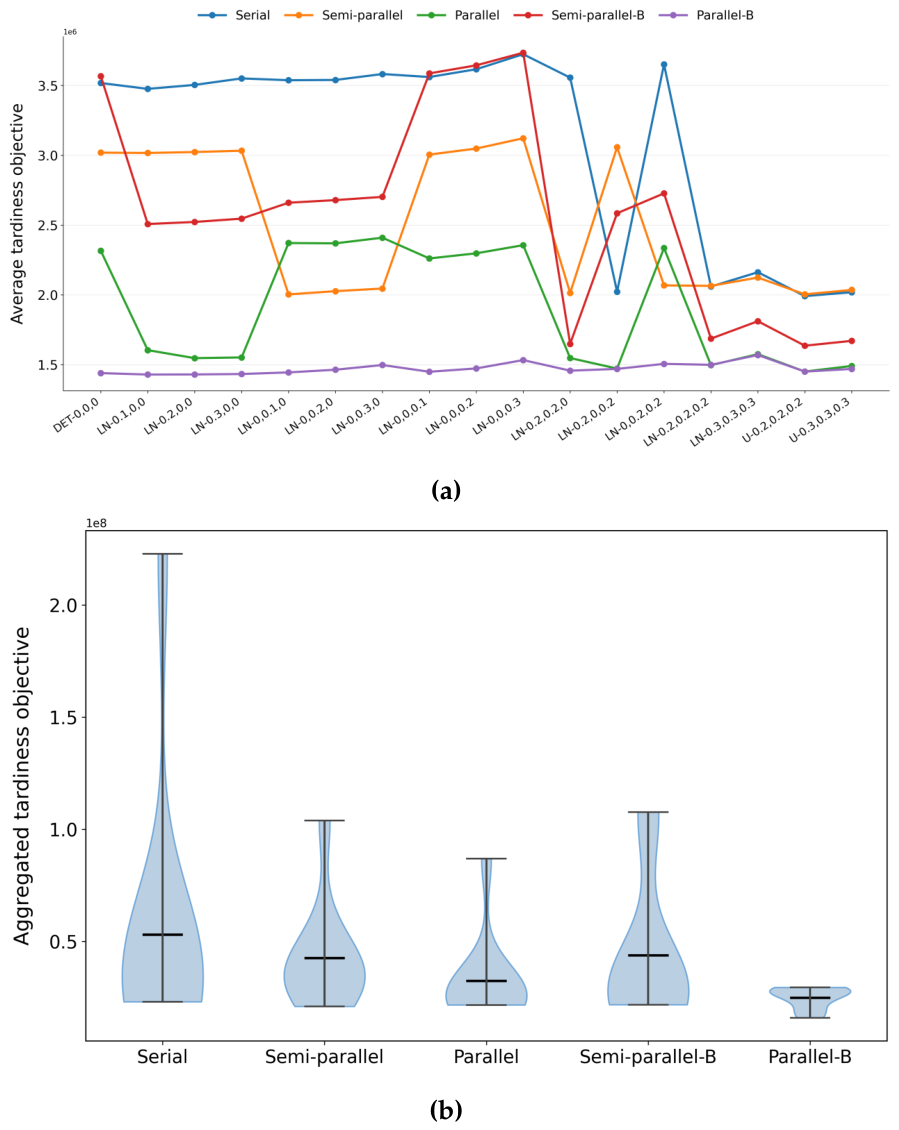
Figure 5.
Relative frequencies of terminal nodes used in the evolved priority functions for each routing strategy and optimization objective.
Figure 5.
Relative frequencies of terminal nodes used in the evolved priority functions for each routing strategy and optimization objective.
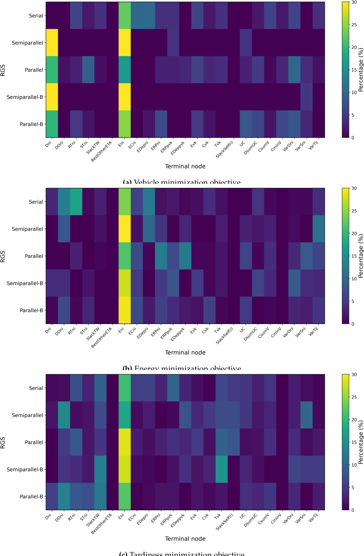
Figure 6.
Correlation between terminal node usage frequency and objective values for each routing strategy and optimization objective. The values represent Spearman rank correlation coefficients. Only correlations with are shown. Statistically stronger correlations () are marked with a red asterisk.
Figure 6.
Correlation between terminal node usage frequency and objective values for each routing strategy and optimization objective. The values represent Spearman rank correlation coefficients. Only correlations with are shown. Statistically stronger correlations () are marked with a red asterisk.
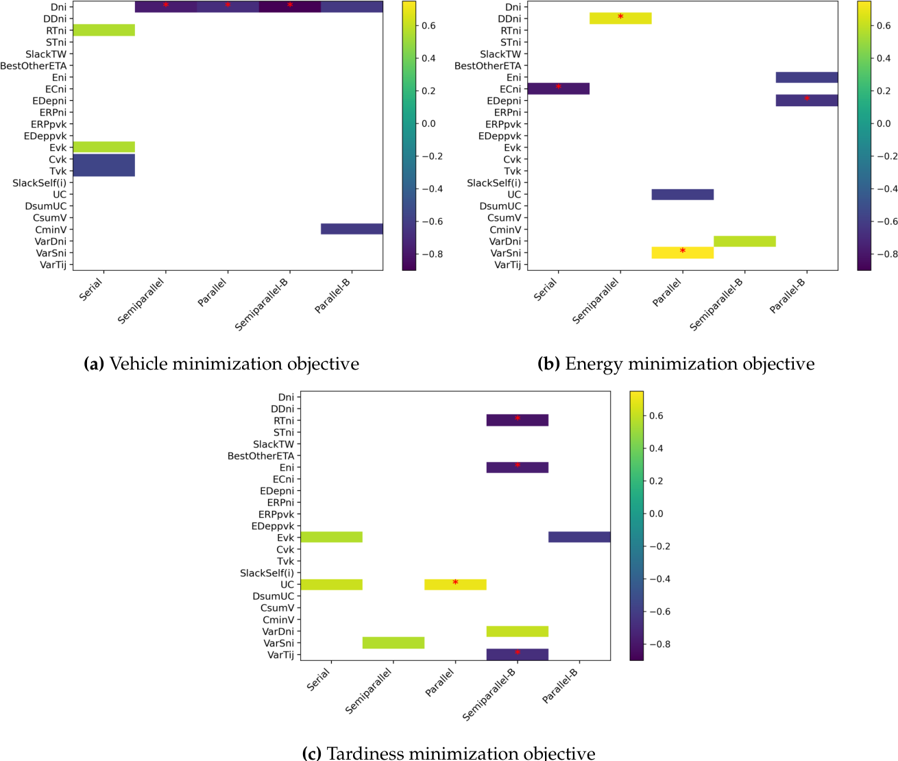
Figure 7.
Comparison between the proposed GP-based routing policies and simple greedy baselines across stochastic scenarios for (a) vehicle minimization, (b) energy minimization, and (c) tardiness minimization objectives. Broken-axis visualization is used in the energy comparison to improve readability due to the large performance gap between methods.
Figure 7.
Comparison between the proposed GP-based routing policies and simple greedy baselines across stochastic scenarios for (a) vehicle minimization, (b) energy minimization, and (c) tardiness minimization objectives. Broken-axis visualization is used in the energy comparison to improve readability due to the large performance gap between methods.
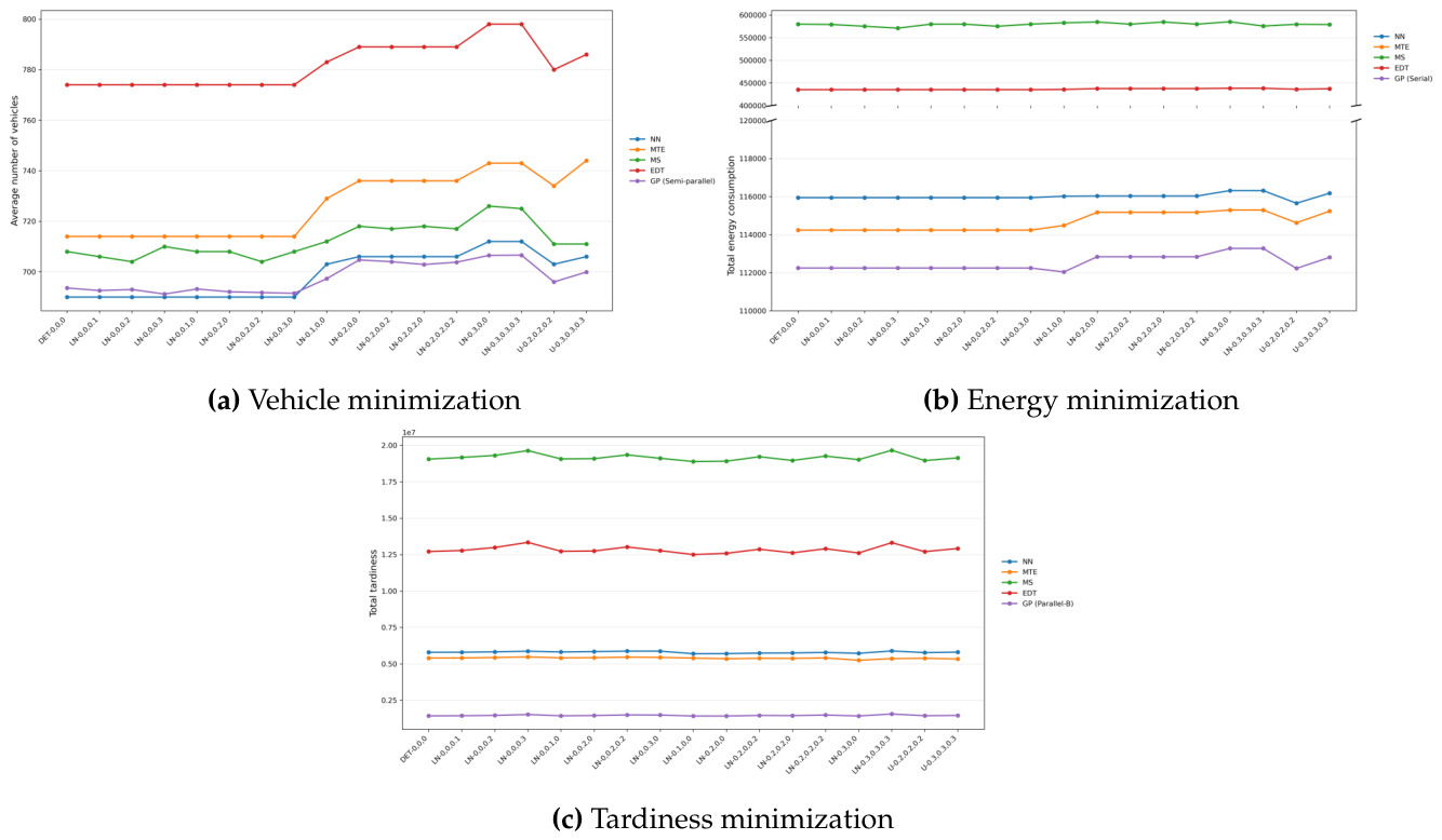

Table 1.
Variant-specific vehicle management rules in the unified RGS framework.
| Variant | Initialization of V | Vehicle selection | Update after route completion |
|---|---|---|---|
| Serial | ∅ | activate a new vehicle | no change |
| Semi-parallel | if , activate a new vehicle; otherwise select the earliest available vehicle from V | ||
| Parallel | select the earliest available vehicle from V | ||
| Semi-parallel-B | if , activate a new vehicle; otherwise select the vehicle with the largest remaining capacity among the K earliest available vehicles in V | ||
| Parallel-B | select the vehicle with the largest remaining capacity among the K earliest available vehicles in V |
Note:V denotes the set of currently active vehicles, and denotes the vehicle whose route has just been completed.
Table 2.
Configuration of the GP algorithm.
| Parameter | Value |
|---|---|
| Initialization | Full |
| Population size | 200 |
| Number of generations | 1000 |
| Initial tree depth | 5 |
| Maximum tree depth | |
| Elitism | 1 |
| Survivor selector | Tournament selection (size 3) |
| Offspring selector | Tournament selection (size 3) |
| Offspring fraction | 0.05 |
| Crossover operator | Subtree crossover |
| Mutation operator | Subtree mutation |
| Mutation rate | 0.2 |
Table 3.
Terminal nodes used in the GP representation.
| Terminal | Objective | Description |
|---|---|---|
| all | Energy required to visit customer i. | |
| all | Demand of customer i. | |
| all | Due time of customer i. | |
| all | Service time of customer i. | |
| all | Ready time of customer i. | |
| all | Remaining battery charge of vehicle k. | |
| all | Remaining cargo capacity of vehicle k. | |
| all | Current route time of vehicle k. | |
| all | Energy required to travel from node i to the centroid of unserved customers. | |
| all | Energy required to travel from node i to the nearest charging station. | |
| all | Energy required to travel from node i to the depot. | |
| all | Energy required to travel from the current position p of vehicle k to the nearest charging station. | |
| all | Energy required to travel from the current position p of vehicle k to the depot. | |
| all | Demand variability parameter for customer i. | |
| all | Travel-time variability parameter for customer i. | |
| all | Service time variability parameter for customer i. | |
| all | Remaining time window slack for customer i. | |
| all | Number of unserved customers. | |
| all | Total demand of all unserved customers. | |
| all | Total remaining capacity of all active vehicles. | |
| all | Minimum estimated arrival time to customer i among the K earliest available vehicles excluding the currently considered vehicle. | |
| vehicle | Minimum remaining capacity among all active vehicles. | |
| tardiness | Available slack of the currently considered vehicle for customer i, computed as the difference between the customer’s due time and the estimated arrival time of the vehicle. |
Table 4.
Function nodes used in the GP representation.
| Function nodes | ||||||
|---|---|---|---|---|---|---|
| add | sub | mul | div | max | min | |
| neg | pow2 | sqr | exp | log | max0 | min0 |
Note: and .
Table 5.
Results for the vehicle minimization objective across all test scenarios. Objective values are aggregated over all 108 runs, yielding a single score for each PF. Best average results are shown in bold.
Table 5.
Results for the vehicle minimization objective across all test scenarios. Objective values are aggregated over all 108 runs, yielding a single score for each PF. Best average results are shown in bold.
| Test Type | Serial | Semi-parallel | Parallel | Semi-parallel-B | Parallel-B | ||||||||||
|---|---|---|---|---|---|---|---|---|---|---|---|---|---|---|---|
| min | max | avg | min | max | avg | min | max | avg | min | max | avg | min | max | avg | |
| DET-0,0,0 | 690 | 708 | 706.2 | 690 | 702 | 693.6 | 714 | 906 | 780.0 | 690 | 696 | 692.4 | 708 | 846 | 742.2 |
| LN-0.1,0,0 | 706 | 710 | 707.7 | 691 | 710 | 697.3 | 725 | 912 | 792.2 | 694 | 712 | 702.9 | 721 | 768 | 735.3 |
| LN-0.2,0,0 | 710 | 714 | 711.7 | 700 | 713 | 704.7 | 728 | 912 | 801.5 | 701 | 712 | 706.0 | 727 | 776 | 737.5 |
| LN-0.3,0,0 | 714 | 723 | 718.6 | 702 | 715 | 706.5 | 743 | 917 | 814.0 | 701 | 719 | 709.4 | 740 | 787 | 753.1 |
| LN-0,0.1,0 | 690 | 708 | 706.2 | 690 | 700 | 693.2 | 710 | 881 | 777.6 | 690 | 699 | 693.6 | 706 | 817 | 735.0 |
| LN-0,0.2,0 | 690 | 708 | 706.2 | 690 | 697 | 692.1 | 719 | 881 | 777.7 | 690 | 697 | 692.8 | 707 | 833 | 738.1 |
| LN-0,0.3,0 | 690 | 708 | 706.2 | 690 | 695 | 691.5 | 718 | 872 | 776.6 | 690 | 697 | 692.8 | 708 | 823 | 736.7 |
| LN-0,0,0.1 | 690 | 708 | 706.2 | 690 | 698 | 692.6 | 721 | 802 | 763.7 | 690 | 695 | 692.0 | 711 | 830 | 738.9 |
| LN-0,0,0.2 | 690 | 708 | 706.2 | 690 | 700 | 693.0 | 710 | 806 | 763.8 | 690 | 701 | 694.4 | 712 | 829 | 742.0 |
| LN-0,0,0.3 | 690 | 708 | 706.2 | 690 | 694 | 691.2 | 724 | 802 | 765.8 | 690 | 698 | 693.2 | 714 | 821 | 740.5 |
| LN-0.2,0.2,0 | 710 | 714 | 711.7 | 699 | 710 | 702.9 | 728 | 890 | 798.1 | 700 | 715 | 706.8 | 723 | 772 | 737.5 |
| LN-0.2,0,0.2 | 710 | 714 | 711.7 | 699 | 713 | 704.0 | 737 | 833 | 788.3 | 700 | 710 | 704.2 | 729 | 774 | 741.5 |
| LN-0,0.2,0.2 | 690 | 708 | 706.2 | 690 | 696 | 691.8 | 723 | 799 | 762.3 | 690 | 695 | 692.0 | 714 | 824 | 743.0 |
| LN-0.2,0.2,0.2 | 710 | 714 | 711.7 | 700 | 712 | 703.8 | 740 | 829 | 788.7 | 701 | 712 | 705.4 | 726 | 776 | 737.4 |
| LN-0.3,0.3,0.3 | 714 | 723 | 718.6 | 702 | 716 | 706.6 | 749 | 846 | 806.3 | 702 | 720 | 710.4 | 745 | 786 | 753.2 |
| U-0.2,0.2,0.2 | 702 | 710 | 704.8 | 693 | 701 | 696.0 | 724 | 811 | 773.6 | 693 | 704 | 699.1 | 716 | 774 | 731.6 |
| U-0.3,0.3,0.3 | 706 | 713 | 709.5 | 696 | 707 | 699.9 | 722 | 823 | 782.0 | 694 | 707 | 701.5 | 722 | 774 | 733.2 |
Table 6.
Results for the energy minimization objective across all test scenarios. Values are aggregated over all 108 runs for each PF. Best average results are highlighted in bold.
Table 6.
Results for the energy minimization objective across all test scenarios. Values are aggregated over all 108 runs for each PF. Best average results are highlighted in bold.
| Test Type | Serial | Semi-parallel | Parallel | Semi-parallel-B | Parallel-B | ||||||||||
|---|---|---|---|---|---|---|---|---|---|---|---|---|---|---|---|
| min | max | avg | min | max | avg | min | max | avg | min | max | avg | min | max | avg | |
| DET-0,0,0 | 109483 | 114402 | 112247 | 123021 | 285645 | 145549 | 126379 | 243339 | 152109 | 122341 | 382873 | 154240 | 125145 | 347641 | 208250 |
| LN-0.1,0,0 | 108269 | 114486 | 112039 | 122821 | 156762 | 129853 | 126186 | 245353 | 152935 | 122285 | 249329 | 141168 | 127278 | 341061 | 185308 |
| LN-0.2,0,0 | 108246 | 115485 | 112838 | 123006 | 156816 | 130064 | 127114 | 245361 | 153378 | 121558 | 252270 | 141641 | 127499 | 341129 | 185888 |
| LN-0.3,0,0 | 109163 | 115294 | 113277 | 122679 | 156694 | 130090 | 127749 | 244700 | 153715 | 121368 | 253036 | 141805 | 127488 | 339883 | 185790 |
| LN-0,0.1,0 | 109483 | 114402 | 112247 | 122101 | 285901 | 144555 | 126443 | 169749 | 141132 | 117934 | 143217 | 127476 | 126213 | 345687 | 175921 |
| LN-0,0.2,0 | 109483 | 114402 | 112247 | 121732 | 289683 | 144898 | 127429 | 167777 | 141424 | 116793 | 143584 | 127346 | 126252 | 343628 | 174911 |
| LN-0,0.3,0 | 109483 | 114402 | 112247 | 121763 | 288712 | 144709 | 127551 | 168641 | 141767 | 116999 | 140757 | 126917 | 125747 | 342225 | 174808 |
| LN-0,0,0.1 | 109483 | 114402 | 112247 | 121495 | 283259 | 140133 | 128816 | 253226 | 153183 | 120255 | 361474 | 151889 | 125322 | 344273 | 186094 |
| LN-0,0,0.2 | 109483 | 114402 | 112247 | 120382 | 286223 | 140043 | 129219 | 272935 | 155101 | 119585 | 367630 | 152299 | 126187 | 341690 | 185531 |
| LN-0,0,0.3 | 109483 | 114402 | 112247 | 121541 | 286588 | 140834 | 128674 | 285961 | 156435 | 120852 | 370378 | 152897 | 124422 | 342404 | 185365 |
| LN-0.2,0.2,0 | 108246 | 115485 | 112838 | 122185 | 154202 | 129327 | 128405 | 170164 | 142399 | 117992 | 142122 | 127596 | 127734 | 339960 | 154014 |
| LN-0.2,0,0.2 | 108246 | 115485 | 112838 | 120664 | 129064 | 124752 | 129837 | 273548 | 156153 | 118915 | 264442 | 142507 | 127539 | 342366 | 165048 |
| LN-0,0.2,0.2 | 109483 | 114402 | 112247 | 120511 | 287623 | 139797 | 129272 | 145603 | 138785 | 119642 | 144846 | 127719 | 125279 | 346369 | 153192 |
| LN-0.2,0.2,0.2 | 108246 | 115485 | 112838 | 120198 | 128676 | 124632 | 130533 | 147318 | 139879 | 119934 | 140901 | 127653 | 126960 | 142402 | 132474 |
| LN-0.3,0.3,0.3 | 109163 | 115294 | 113277 | 122533 | 129999 | 125350 | 131238 | 146756 | 140313 | 120981 | 141241 | 128441 | 128252 | 143526 | 133382 |
| U-0.2,0.2,0.2 | 107853 | 114624 | 112226 | 121031 | 128955 | 124411 | 128322 | 146893 | 139145 | 119918 | 144009 | 127811 | 125738 | 143700 | 131530 |
| U-0.3,0.3,0.3 | 108220 | 115237 | 112807 | 122534 | 128672 | 124593 | 129172 | 147238 | 139344 | 119287 | 141759 | 127395 | 126633 | 144245 | 132269 |
Table 7.
Results for the tardiness minimization objective across all test scenarios. Values are aggregated over all 108 runs for each PF. Best average results are highlighted in bold.
Table 7.
Results for the tardiness minimization objective across all test scenarios. Values are aggregated over all 108 runs for each PF. Best average results are highlighted in bold.
| Test Type | Serial | Semi-parallel | Parallel | Semi-parallel-B | Parallel-B | ||||||||||
|---|---|---|---|---|---|---|---|---|---|---|---|---|---|---|---|
| min | max | avg | min | max | avg | min | max | avg | min | max | avg | min | max | avg | |
| DET-0,0,0 | 1272858 | 17454211 | 3517394 | 1210110 | 11028856 | 3018684 | 1250509 | 8716784 | 2315090 | 1308559 | 11171014 | 3566337 | 930297 | 1695840 | 1439120 |
| LN-0.1,0,0 | 1295728 | 17202117 | 3475506 | 1206817 | 10989757 | 3016350 | 1240738 | 2849206 | 1603646 | 1219902 | 11033621 | 2507362 | 917330 | 1706153 | 1428824 |
| LN-0.2,0,0 | 1336054 | 17399316 | 3504015 | 1215753 | 10981193 | 3022953 | 1224670 | 2844094 | 1546361 | 1199907 | 11150831 | 2521950 | 887459 | 1716387 | 1429511 |
| LN-0.3,0,0 | 1361288 | 17711092 | 3550482 | 1242329 | 10997206 | 3032523 | 1213094 | 2792692 | 1551372 | 1229698 | 11049623 | 2545836 | 899188 | 1736667 | 1432600 |
| LN-0,0.1,0 | 1343420 | 17496136 | 3537530 | 1213993 | 3325752 | 2002971 | 1271442 | 9289961 | 2370938 | 1283278 | 11309917 | 2659916 | 975003 | 1680049 | 1444139 |
| LN-0,0.2,0 | 1371227 | 17506482 | 3539480 | 1253590 | 3315177 | 2026268 | 1297806 | 9262846 | 2368827 | 1287342 | 11312963 | 2678580 | 955569 | 1743110 | 1463359 |
| LN-0,0.3,0 | 1394990 | 17506469 | 3581873 | 1270528 | 3385246 | 2045000 | 1308235 | 9531344 | 2409334 | 1370673 | 11287970 | 2701728 | 988302 | 1777852 | 1497089 |
| LN-0,0,0.1 | 1312666 | 17622550 | 3560397 | 1177200 | 10885939 | 3004804 | 1254014 | 9112611 | 2260626 | 1285101 | 11290638 | 3586483 | 939299 | 1686971 | 1448779 |
| LN-0,0,0.2 | 1334679 | 17981679 | 3616232 | 1213344 | 10957581 | 3047969 | 1258336 | 9322957 | 2297374 | 1315652 | 11383860 | 3644094 | 955893 | 1713679 | 1472615 |
| LN-0,0,0.3 | 1361615 | 18627900 | 3723803 | 1265949 | 11273473 | 3121683 | 1334622 | 9369931 | 2355746 | 1361115 | 11661684 | 3734739 | 1006265 | 1783310 | 1532400 |
| LN-0.2,0.2,0 | 1389772 | 17535696 | 3555869 | 1244420 | 3292794 | 2013154 | 1291612 | 2699803 | 1547006 | 1245622 | 2052893 | 1648394 | 896188 | 1760556 | 1456583 |
| LN-0.2,0,0.2 | 1343215 | 2536512 | 2022343 | 1223754 | 10962810 | 3057451 | 1208560 | 1808946 | 1471642 | 1202368 | 11312763 | 2584319 | 937424 | 1758931 | 1469182 |
| LN-0,0.2,0.2 | 1388800 | 18131391 | 3651489 | 1276945 | 3387660 | 2067709 | 1329592 | 9583996 | 2334982 | 1323947 | 11447690 | 2727041 | 991492 | 1751834 | 1505385 |
| LN-0.2,0.2,0.2 | 1396523 | 2603891 | 2059124 | 1267127 | 3386941 | 2064047 | 1311832 | 1812573 | 1496135 | 1299616 | 2102893 | 1686141 | 928650 | 1809302 | 1498555 |
| LN-0.3,0.3,0.3 | 1504091 | 2703198 | 2161896 | 1342451 | 3379428 | 2123752 | 1372330 | 1855124 | 1574805 | 1352172 | 2136361 | 1810874 | 977262 | 1862499 | 1568568 |
| U-0.2,0.2,0.2 | 1358960 | 2525524 | 1990790 | 1200782 | 3353498 | 2003330 | 1222586 | 1729881 | 1450297 | 1278533 | 2003868 | 1635515 | 892732 | 1711353 | 1449908 |
| U-0.3,0.3,0.3 | 1369182 | 2587591 | 2018648 | 1253462 | 3423508 | 2035246 | 1266529 | 1768924 | 1490303 | 1267831 | 1991775 | 1670210 | 939074 | 1756884 | 1469011 |
Table 8.
Pairwise Wilcoxon signed-rank tests with Holm correction for the three objectives. indicates a statistically significant difference (p < 0.05). Exact p-values are reported only for non-significant comparisons.
Table 8.
Pairwise Wilcoxon signed-rank tests with Holm correction for the three objectives. indicates a statistically significant difference (p < 0.05). Exact p-values are reported only for non-significant comparisons.
| Objective | Method | Serial | Semi-parallel | Parallel | Semi-parallel-B | Parallel-B |
|---|---|---|---|---|---|---|
| Vehicles | Serial | – | ||||
| Semi-parallel | – | |||||
| Parallel | – | |||||
| Semi-parallel-B | – | |||||
| Parallel-B | – | |||||
| Energy | Serial | – | ||||
| Semi-parallel | – | |||||
| Parallel | – | |||||
| Semi-parallel-B | – | |||||
| Parallel-B | – | |||||
| Tardiness | Serial | – | ||||
| Semi-parallel | – | |||||
| Parallel | – | |||||
| Semi-parallel-B | – | |||||
| Parallel-B | – |
Disclaimer/Publisher’s Note: The statements, opinions and data contained in all publications are solely those of the individual author(s) and contributor(s) and not of MDPI and/or the editor(s). MDPI and/or the editor(s) disclaim responsibility for any injury to people or property resulting from any ideas, methods, instructions or products referred to in the content. |
© 2026 by the authors. Licensee MDPI, Basel, Switzerland. This article is an open access article distributed under the terms and conditions of the Creative Commons Attribution (CC BY) license.
Copyright: This open access article is published under a Creative Commons CC BY 4.0 license, which permit the free download, distribution, and reuse, provided that the author and preprint are cited in any reuse.


