

Submitted:
21 May 2026
Posted:
22 May 2026
You are already at the latest version
Abstract
As extreme heat events increase in frequency, intensity, and duration due to climate change, forecasting these events has become vital for early warning systems, public health preparedness, and climate adaptation strategies, especially in the hottest parts of the world. In recent years, machine learning (ML) has increasingly been applied to environmental and meteorological data to improve the prediction of heatwaves and extreme heat events. This scoping review examines global peer-reviewed literature on the application of ML techniques for extreme heat prediction using environmental variables. This includes heatwave prediction, environmental and meteorological predictors used in these models, and the geographical distribution of existing research. A total of 23 peer-reviewed studies meeting the inclusion criteria were included in the review, following the PRISMA-ScR guidelines. The findings indicate that artificial neural networks and random forest models are among the most frequently reported high-performing approaches for heatwave prediction. Temperature-related variables, especially maximum temperatures, were consistently identified as the most influential predictors across studies. Furthermore, the evidence base was heavily concentrated in Europe and North America, with comparatively limited representation from low- and middle-income countries, despite these regions often experiencing disproportionate impacts of climate change and extreme heat exposure. By synthesising current evidence on ML-based heatwave prediction, associated environmental predictors, and geographical research trends, this review provides insights to support the development of more robust, context-aware, and globally representative heatwave forecasting frameworks.
Keywords:
artificial intelligence
; machine learning
; heatwave prediction
; environmental exposure
; climate change
; scoping review
1. Introduction
Climate change is contributing to a substantial increase in the frequency, duration, and intensity of extreme heat events worldwide, posing serious threats to human health, society, and the environment [1,2]. Heatwaves are now recognised as one of the most hazardous climate-related events, contributing significantly to excess mortality, heat-related illnesses, and increased pressure on healthcare systems, particularly among vulnerable populations, such as older adults, children, and individuals with pre-existing health conditions [1,3]. Therefore, accurate prediction of heatwave events is essential to support early warning systems, enable timely public health interventions, and strengthen preparedness and emergency response strategies.
In recent years, machine learning (ML) approaches have been increasingly applied in environmental and climate sciences, demonstrating substantial potential in areas such as weather forecasting [4], climate change mitigation and adaptation [5], and the prediction of extreme atmospheric events [6]. This rapid expansion has been facilitated by the growing availability of large observational, reanalysis, and remote sensing datasets, which provide the high-volume, multi-source inputs required for data-driven models to learn complex and nonlinear relationships without explicit physical parameterisation [7]. These characteristics make ML approaches particularly suitable for predicting rare but high-impact climate-sensitive events, such as heatwaves, where traditional physics-based numerical weather prediction systems may face limitations in forecast skill and computational efficiency [4,8]. Therefore, a growing body of research has applied ML techniques to the prediction of extreme heat events [9,10,11]. However, these studies differ considerably in their methodological choices, geographical coverage, predictor variables, and reported performance metrics, making it difficult to draw generalisable conclusions about which modelling approaches and environmental inputs are most effective [9].
Some studies have reviewed ML-based heatwave classification within specific national contexts [9,11,12], while a broader assessment of heatwave predictability across temporal scales has discussed ML approaches only partially within a wider meteorological framework [13]. Other reviews have addressed ML applications in weather forecasting more generally without focusing specifically on heat events [14,15], or have examined atmospheric extremes collectively, including floods, droughts, and temperature events, without synthesising comparative evidence on ML model performance for heatwave prediction [6]. Despite the growing research on ML-based heatwave prediction, studies have been conducted predominantly in high-income countries (HIC) settings, with low- and middle-income countries (LMICs) remaining largely absent from the literature [16,17]. This geographical imbalance is especially consequential given that the heat stress burden and heatwave-associated mortality risk are escalating at a disproportionately faster rate in lower-income settings [18,19]. While some reviews have examined algorithm use or predictor selection within specific domains [9,17], none have simultaneously focused exclusively on heatwave or extreme heat prediction, adopted a global scope inclusive of LMIC settings, and systematically characterised both the ML algorithms employed and the environmental predictors used as model inputs across studies.
This review directly addresses these gaps in the literature. By mapping and synthesising the global literature on ML-based heatwave prediction, it provides a systematic characterisation of both the algorithms employed and the environmental predictors used as model inputs across studies, regions, and prediction horizons. Unlike previous reviews, it encompasses studies from both HIC and LMIC settings and synthesises performance evidence to provide algorithm-level insights rather than a descriptive summary alone. The review has three primary objectives: (1) to identify and characterise the ML algorithms that have been applied to the prediction of heat events; (2) to identify which environmental parameters have been used as predictors in those models and to assess the available evidence regarding their relative importance; and (3) to examine the geographical distribution of existing studies.
2. Methods
A scoping review was conducted to identify key environmental parameters and ML models used to predict and forecast extreme heat. A scoping review was chosen as they are suitable for mapping a heterogeneous body of literature and identifying gaps [20]. A review protocol was developed and made publicly available on the Open Science Framework [21]. The protocol and conduct of the scoping review followed the Preferred Reporting Items for Systematic Reviews and Meta-Analyses extension for Scoping Reviews (PRISMA-ScR) guidelines [20].
2.1. Eligibility Criteria
Studies were included if they met the following criteria:
- 1.
- Studies must involve the use of machine learning to predict periods of extreme heat.
- 2.
- Studies must include descriptions of what machine learning methods or parameters were used to make predictions.
- 3.
- Studies must be original peer-reviewed research.
- 4.
- Studies must be in English.
- 5.
- Both indoor and outdoor temperature predictions were included.
- 6.
- There are no restrictions on geographical location.
- 7.
- There are no restrictions on publication date, as preliminary searches found limited relevant literature before 2020.
Studies were excluded if they met the following criteria:
- 1.
- Predictions of the effects of heatwaves on human, plant, or animal health.
- 2.
- Impacts of weather on infrastructure and transport.
- 3.
- Extremely long-term weather and climate predictions.
- 4.
- Oceanic temperature predictions.
- 5.
- Weather predictions other than extreme heat, including flooding and water levels.
- 6.
- Developing weather-related technologies.
2.2. Information Sources and Search Strategy
A structured literature search was conducted across multiple bibliographic databases, including the Web of Science Core Collection, ACM Digital Library, Scopus, IEEE Xplore, and ScienceDirect. An initial exploratory search was performed in March 2025 to refine the key concepts, search terms, and database suitability. Based on these results, the search strategy was iteratively refined through discussions with senior researchers and academic librarians at the University of the West of Scotland, leading to a final comprehensive search conducted in July 2025.
The search terms were developed around four core components: extreme heat exposure, ML or artificial intelligence (AI) methods, prediction tasks, and environmental or weather-related parameters. Controlled vocabulary and free text terms were combined using Boolean operators, truncation, and proximity operators, where supported. Search syntax was adapted for each database to account for differences in indexing fields, operators, and search functionalities. An example of the full search strategy used for the Web of Science database, including search components and syntax, is presented in Table 1. Full details of the database-specific search strategies and refinement procedures are provided in Supplementary File S1.
2.3. Selection of Study
All retrieved records were exported from the databases and imported into Rayyan, a web-based platform for managing reviews [22], for citation management, duplicate removal, screening, and data extraction. The initial screening was independently performed by two reviewers (AA and FA) based on the predefined eligibility criteria. Any disagreements were resolved through discussion and consensus, with consultation with a third reviewer (MZS) where required. Citations meeting the inclusion criteria progressed to full-text assessment, which was conducted by two reviewers using the same eligibility criteria.
2.4. Data Extraction and Synthesis
Data extraction was performed on full-text articles using Rayyan, with extracted data subsequently organised in an Excel spreadsheet. Extraction was performed by two extractors (AA and FA) working independently. The results were then combined. Data were extracted into a structured spreadsheet with the following key fields:
- Country, geographical coverage
- Prediction target
- Heatwave definition, extreme heat definition
- Environmental predictors, non-environmental predictors, derived indices
- ML models, best model
- Performance metrics, best model performance
- Validation method
- Key findings
- Limitations of study

Table 1.
An example of a Web of Science search strategy.
| Search Component | Search Syntax (TITLE-ABS-KEY) |
|---|---|
| Extreme heat terms | (“Extreme heat” OR “Extreme weather even” OR heatwave* OR “thermal comfort”) |
| AI and ML terms | (“Machine learning” OR “Artificial intelligence” OR “Neural network” OR “Deep learning” OR “Support Vector Machine” OR “Random Forest”) |
| Prediction terms | (Predict* OR Forecast* OR modeling) |
| Environmental Predictors | (environmental NEAR/3 parameters OR temperature OR humidity OR weather NEAR/3 data) |
| Combined search strategy | TS=((“Extreme heat” OR “Extreme weather event” OR heatwave* OR “thermal comfort”) AND (“Machine learning” OR “Artificial intelligence” OR “Neural network” OR “Deep learning” OR “Support Vector Machine” OR “Random Forest”) AND (Predict* OR Forecast* OR modeling) AND (environmental NEAR/3 parameters OR temperature OR humidity OR weather NEAR/3 data)) AND (DT=(Article)) |
Following data extraction, findings were synthesised qualitatively to describe study characteristics, including geographical coverage, study settings, definitions of extreme heat, risks assessed, environmental parameters, ML techniques, and validation approaches. Due to heterogeneity in ML methods and outcomes, no quantitative synthesis or meta-analysis was performed. A detailed data extraction table is provided in Supplementary File S2.
3. Results
The database searches identified 860 records in total. After the removal of 83 duplicate records, 777 unique citations were screened by title and abstract. Following this initial screening, 83 articles were assessed at the full-text level, of which 23 studies met the eligibility criteria and were included in the scoping review. The study selection process is illustrated in the PRISMA flow diagram in Figure 1. The 23 included studies are summarised in Table 2 according to the prediction target, key predictors, best performing ML model, validation methods used, and key findings.
3.1. Geographic Coverage and Study Settings
Of the 23 studies included in this review, ten were conducted in Asia (43.5%), with studies reported from India [24,30,38,42], Japan [44], Pakistan [31,40], Bangladesh [27], Thailand [28], and Taiwan [33]. Eight studies (34.8%) were based in Europe, covering France [29,34,41], Spain [26,29], Germany and Switzerland [41], Italy [35], and the United Kingdom [43], as well as broader regional analyses covering Europe or Eastern Europe [36,45]. Four studies (17.4%) were conducted in North America, specifically the United States [25,32,37] and Canada [23], and one study was conducted in Australia (4.3%) [39]. No studies were identified from Africa, South America, or Central America. The geographical distribution of the included studies across countries is illustrated in Figure 2, while the temporal distribution of publications by continent is presented in Figure 3, which highlights a notable increase in research output from 2022 onwards, particularly in the Asian and European contexts. Data were collected at varying administrative scales, including continental, national, regional, and municipal levels.
3.2. Heat-Related Prediction Targets
The 23 included studies differed in their ML prediction targets, reflecting the different operational definitions of heat-related hazards. As shown in Figure 4, the most common objective was the prediction of heatwave occurrence or onset, reported in eight studies [24,28,31,32,34,36,42,45]. Seven studies focused on predicting periods of extreme heat without applying a formal heatwave definition [27,33,37,38,39,40,44]. Four studies focused on predicting ambient air temperature as a continuous variable [25,26,29,30], while one study specifically examined nocturnal temperature patterns [35]. In addition, three studies predicted indoor temperature [23,41,43], highlighting applications related to building environments and indoor heat exposure.
3.3. Heatwave and Extreme Heat Definitions Across Studies
Substantial variation was observed in the definition of heatwaves and extreme heat across the included studies. Ten studies used an explicit percentile threshold-based definition [23,24,28,31,32,33,34,35,40,45], five used an absolute temperature threshold [26,41,42,43,44], and eight predicted continuous temperature variables without defining discrete heatwave events [25,27,29,30,36,37,38,39]. Among the studies that provided percentile-based definitions, five defined heatwaves using the 90th percentile of daily Tmax as the main criterion [28,32,33,35,45]. However, the minimum duration required to classify a heatwave varies from three consecutive days [28,32,35] to six days [45]. Four studies used the 95th percentile threshold [24,31,34,40], with one translating this into an absolute value of 41°C for the study region [40], and one using a space-time averaged temperature anomaly instead of a station-level threshold [34]. Another study applied the 97th percentile of a 3-day rolling average temperature, corresponding to 21.5°C, illustrating how percentile-based definitions depend on the climatic context, particularly in cooler regions [23]. Five studies used an absolute temperature threshold to define heatwaves, with thresholds ranging from 26°C to 40°C, depending on the climatic and regulatory context of the study region [26,35,41,43,44]. In some cases, thresholds were derived from national meteorological or occupational safety standards, while in others, they varied within countries to account for sub-regional climatic differences. One additional study defined extreme heat using maximum temperature anomalies of 4°C or above relative to a climatological baseline [38], further highlighting the heterogeneity in operational definitions beyond the percentile-based approach described above.
3.4. Environmental Predictors and Derived Indices
Environmental predictors used across the included studies comprised meteorological, land surface, and large-scale climate variables, alongside engineered features derived from these inputs. Figure 5 summarises the frequency of temperature and thermal variables (panel A), other environmental predictors (panel B), feature engineering approaches (panel C), and the distribution of predictor counts per study (panel D), while detailed study-level information is provided in the supplementary file S2.
3.4.1. Temperature and Thermal Variables
Temperature variables were used as predictors in 20 of the 23 studies. Air temperature, 2-m temperature (T2M), or mean temperature was used as a model input in 12 studies [23,26,27,28,29,32,34,36,37,39,41,43], whereas daily maximum temperature (Tmax) was used explicitly as a predictor input in eight studies [23,26,27,28,29,33,36,40] and as a prediction target only in seven studies [24,30,31,32,38,42,45]. The daily minimum temperature (Tmin) was used as a predictor input in three studies [28,32,40]. Satellite-derived land surface temperature (LST) was incorporated as a predictor in three studies [25,28,35]. Indoor air temperature was used in three studies [23,41,43], and temperature anomalies were constructed as predictor inputs in four studies [34,36,38,45]. Thermal comfort and exposure indices were used in four studies: Physiologically Equivalent Temperature (PET and PETi) [41], sol-air temperature [23], indoor overheating metric (TOH) [43], and Mean Radiant Temperature (MRT) [44]. Heatwave characteristics derived from temperature thresholds, including frequency, duration, magnitude, and number, were reported in one study [28].
3.4.2. Other Environmental Predictors
Humidity and moisture variables, including relative humidity, dew point temperature, and vapour pressure, were reported in 11 studies [23,24,27,31,32,37,39,40,41,42,43]. Wind speed or direction was included in 10 studies [23,24,27,31,32,36,39,40,41,42], as were surface or sea-level pressure variables reported in eight studies [24,27,31,32,36,40,41,42]. Solar and longwave radiation were reported in five studies [23,24,41,42,44], and precipitation-related variables, including rainfall, snow cover, and sea ice in five studies [30,32,37,40,45]. Geopotential height (Z200 or Z500) was incorporated in six studies [24,27,31,34,36,38], sea surface temperature (SST) in four studies [24,36,38,45], and soil moisture in four studies [24,34,38,45]. Land cover, urban morphology, and building-related variables were included in four studies [23,25,28,43]. Air pollution variables, including aerosol optical depth (AOD), black carbon (BC), carbon monoxide (CO), and particulate matter, have been reported in one study [42].
3.4.3. Feature Engineering and Predictor Selection
Fifteen of the 23 studies applied feature engineering approaches beyond the direct use of raw environmental inputs. Lag and temporal window features were used in six studies [23,26,31,32,33,41], with temporal windows ranging from hourly lags (t-1 h to t-24 h) [41] to multistep sequences including 30 successive hourly steps [26] and daily windows of one to ten days [31,33]. Signal decomposition was applied in two studies, including ensemble empirical mode decomposition producing 11 intrinsic mode functions with a residual trend [33], and recurrence plot representations used as convolutional neural network inputs [29]. Spatial averaging or geographic area selection was applied in five studies [24,36,38,39,45], and principal component analysis (PCA) was applied in two studies [36,38]. Climate teleconnection indices, including the oceanic Niño Index and SST-based predictors, were used in two studies [32,38], and physics-informed feature construction was reported in two studies [35,39]. Formal or algorithm predictor selection approaches were applied in nine studies, including correlation-based filtering with stepwise regression [31], Pearson correlation exclusion [35,42], spatial correlation-based region selection [36], correlation filtering combined with PCA [38], global Sobol sensitivity analysis [39], exhaustive feature subset search [29], genetic algorithm optimisation [44], and variable selection analysis [37]. Informal or domain-informed selection approaches were used in six studies [23,24,25,27,28,45], while eight studies reported no predictor selection or screening procedure [26,30,32,33,34,40,41,43]. The number of predictors used per study ranged from 3 to 34, with eight studies using 1-9 predictors, five using 10-19 predictors, and five studies using between 20 and 34 predictors, while five studies did not report counts explicitly, as shown in Figure 5D.
3.5. Machine Learning Approaches
Across the included studies (n=23), a diverse range of shallow, ensemble, and DL models were applied alongside hybrid architectures combining signal processing with NNs or stacking multiple learners. Detailed model configurations, prediction targets, and performance metrics are presented in Table 2, whereas Figure 6 summarises the distribution of model families evaluated across studies and those reported as best-performing (panel A), and the frequency of performance metrics reported across studies (panel B).
3.5.1. Shallow and Ensemble Learning
The number of models evaluated per study ranged from 1 to 13, with 11 studies employing a single model, six studies evaluating two models, two studies evaluating three models, and four studies evaluating four or more models (Supplementary Fig. S1A). Shallow and ensemble learning methods were prominent across the included studies, appearing in 12 of the 23 studies as primary or best-performing models. RF was the most frequently evaluated algorithm, appearing in nine studies [28,29,30,31,35,37,39,42,45], and identified as best-performing in four [28,35,37,42], and was applied across both regression and binary classification tasks. Quantile random forest was found to be effective in predicting the occurence of heatwaves in one study [31], but less effective than ARIMA in another [30].
Gradient Boosting (GB) approaches, including XGBoost, LightGBM, AdaBoost, CatBoost, and GBM, were reported in seven studies [24,29,30,38,42,45]. Within this group, LightGBM outperformed linear regression for heatwave frequency prediction [45], XGBoost achieved a very high predictive performance for high-resolution air temperature mapping [25], and AdaBoost combined with an MLP base estimator emerged as the best-performing model among multiple ensemble configurations for short-term temperature forecasting [38].
Support vector regression was evaluated in three studies [24,42,43] and demonstrated strong short-range performance, although the accuracy declined at longer lead times and in lower-temperature regions [24]. Other shallow approaches, including Lasso regression, DT, and KNNs, were evaluated in two studies [29,30] and were consistently outperformed by ensemble-based methods where comparisons were conducted. GPR was applied as a surrogate modelling approach for WRF outputs rather than as a direct predictive model, identifying a limited subset of influential physical parameters governing heat extremes [39]. When multiple shallow models were compared within the same study, no single algorithm consistently dominated. RF outperformed multiple statistical and ML baselines in several cases, including satellite-derived temperature prediction [42], and downscaled temperature distribution modelling [37]. However, contrasting results were also observed: ARIMA outperformed all evaluated ML models for long-term temperature forecasting [30], whereas CNN-based architectures exceeded the performance of ensemble methods in seasonal prediction tasks [29].
3.5.2. Deep Learning Approaches
Deep learning architectures were applied in 13 of the 23 included studies, spanning feedforward ANN, MLP, CNN, LSTM, GNN, RBFNN hybrids, and autoencoder-based frameworks, as detailed in Table 2, and illustrated in Figure 6A. ANN and MLP variants were the most frequently reported, appearing in eight studies [23,26,27,38,40,41,43,44], and identified as best-performing in six studies [23,26,27,41,43,44]. ANN outperformed time-series regression for indoor thermal prediction [23], exceeded SVM for national-scale indoor overheating estimation [43], and achieved a high predictive accuracy for outdoor mean radiant temperature around buildings [44]. An MLP combining NWP forecasts with indoor sensor data produced an MAE of 0.87K with 91% of predictions within 2K [41], while an MLP trained on crowdsourced citizen weather station data achieved R2 = 0.98 for fine-scale urban temperature distribution [26]. Autoencoder-MLP hybrids extended predictive skill to sub-seasonal horizons of one to four weeks across seven European cities [36]. LSTM was evaluated in one study and achieved the highest classification accuracy reported in this review (96.2%) for one- to three-day extreme heat event prediction, outperforming both CNN and ANN evaluated in the same study [40]. CNN-based architectures were evaluated in two studies [29,34]. A probabilistic CNN demonstrated positive forecast skill to approximately 15 days for extreme heatwave occurrence, outperforming logistic regression baselines [34], whereas a recurrence-plot CNN hybrid outperformed AdaBoost and RF for seasonal temperature prediction and detected the 2003 European heatwave anomaly [29]. GNN was evaluated in one study and achieved an accuracy of 94.1% for binary heatwave classification, with the inclusion of the Oceanic Niño Index improving multi-station prediction [32]. RBFNN combined with signal decomposition was evaluated in one study and achieved correlation coefficients of and RMSE of approximately for temperature forecasting across lead times up to seven days [33].
3.5.3. Validation Strategies and Performance Reporting
The validation approaches varied across the 23 included studies, reflecting differences in data availability, prediction targets, and study design, detailed in Table 2. Train-test splitting was the most commonly applied strategy in nine studies, with five adopting an 80/20 split [27,28,33,40,41], two applying a 70/30 split [24,35], and one applying a 70/15/15 split for training, validation, and testing [23]. CV was applied in five studies: including 3-fold [42], 5-fold [45], 8-fold [39], and 10-fold configurations [25,34]. Temporal splitting, in which earlier observations were used for training and later observations for testing, was applied in seven studies [26,31,32,36,38,44,45], with one study applying LOYO-CV [38], and one study employing both temporal splitting and CV [45]. Three studies evaluated model performance through direct comparison with observed or independently modelled data without a formal holdout strategy [29,30,37], and one study applied simulation-based splitting with 500 runs for training, and 100 for testing [43].
The performance metrics varied across the included studies, as detailed in Table 2, and illustrated in Figure 6. Four studies reported four or more metrics [27,28,29,40], nine reported three [24,26,32,33,35,38,41,43,45], seven reported two [25,30,31,34,36,39,42], and three reported a single metric [23,37,44]. Across all studies, RMSE was the most frequently reported metric, appearing in 13 studies [23,24,25,27,28,30,33,38,39,40,42,43,45], followed by MAE in 10 studies [24,26,28,29,30,35,36,40,41,43], R2 in eight studies [25,26,27,28,35,39,42,43], and MSE in six studies [26,27,29,35,36,40]. Correlation-based measures were reported in five studies [24,31,33,38,41], and classification accuracy in three studies [32,40,44]. Additional evaluation metrics, including probabilistic skill scores [34,37], anomaly correlation coefficients [38], and heatwave detection counts [31], are also detailed in Supplementary Table S2.
3.5.4. Model Explainability and Key Predictors
Explainability methods were applied in 15 of the 23 included studies, with variations in methodological approach and level of implementation (Fig. S1C). Built-in feature importance metrics derived from tree-based models were reported approach, appearing in four studies [28,35,41,45], followed by sensitivity analysis in three studies [32,42,44]. SHAP was applied in two studies [25,40]. Permutation-based importance [38], Sobol global sensitivity analysis [39], and composite map analysis [34] have all been reported in one study. Eight studies reported no formal explainability method [23,24,26,27,29,30,33,36]. Across studies reporting predictor importance, near-surface air temperature and humidity were consistently identified as the most influential inputs, which is consistent with the predictor frequency patterns reported in Section 3.4. SST was identified as the dominant contributor to heatwave frequency prediction, accounting for approximately 70% of the model performance in one study [45]. The geopotential height at 500 hPa was identified as the primary driver of probabilistic heatwave forecast skill at extended lead times [34]. Satellite-derived LST and aerosol optical depth were identified as the strongest predictors in studies incorporating remote sensing inputs [28,42]. Indoor sensor data combined with NWP variables have been reported to improve model interpretability in thermal comfort prediction [41].
4. Discussion
This scoping review was conducted in accordance with the PRISMA-ScR guidelines to systematically map the use of ML approaches for heatwave and extreme heat prediction. A total of 23 studies were included following searches across five major databases and screening of titles, abstracts, and full texts. Collectively, the included studies revealed substantial heterogeneity in study settings, prediction targets, heatwave definitions, environmental predictors, and modelling approaches. Although the application of ML in this domain has increased markedly in recent years, important gaps remain in methodological consistency, predictor diversity, and real-world translation.
4.1. Synthesis of Evidence and Key Patterns
This review identifies substantial methodological and conceptual heterogeneity in the application of ML approaches for heatwave and extreme heat prediction. While all included studies share the overarching objective of predicting heat-related extremes, they differ considerably in prediction targets, including binary heatwave classification, continuous Tmax forecasting, ambient air temperature mapping, and indoor thermal condition modelling. This diversity reflects a broader lack of standardisation in how heat-related prediction problems are formally defined across the literature and complicates the consolidation of evidence and the development of unified modelling frameworks. A similar inconsistency is evident in the operational definitions of heatwaves and extreme heat. The majority of studies (n=10) adopted percentile-based thresholds, typically the 90th or 95th percentile of temperature distributions [23,24,28,31,32,33,34,35,40,45], whereas a smaller subset (n=5) employed absolute temperature thresholds calibrated to national meteorological standards or regional mortality benchmarks [26,41,42,43,44]. In contrast, a further group of studies (n=8) did not report any formal heatwave definition, instead modelling continuous temperature variables, relying on historical extreme events, or using implicit or non-replicable criteria. This variation is closely linked to the geographic and climatic context, as region-specific thresholds are often calibrated to local temperature distributions, population acclimatisation, and national meteorological or public health standards.
Studies conducted in South Asian settings more commonly adopt absolute thresholds derived from established national criteria [40,42], whereas studies in European and North American contexts more frequently apply percentile-based anomaly definitions that accommodate wider inter-regional temperature variability [32,34,45]. However, such contextualisation is necessary if it further complicates cross-regional comparability and limits the development of universally applicable modelling frameworks. Geographically, the evidence base remains unevenly distributed, with ten studies conducted across Asian settings and eight studies in Europe, while four studies were conducted in North America and one study in Australia. No studies were identified in South Africa, South America, or Central America. This imbalance is not incidental, it reflects structural inequalities in research capacity and data infrastructure that systematically exclude the regions bearing the greatest burden of heat-related spatiotemporal predictors [18,19], and it mirrors the geographic concentration documented in prior reviews of ML applications to extreme heat [16]. Collectively, these findings underscore that despite the growing application of machine learning techniques in this domain, the field remains characterised by significant heterogeneity in definitions, predictors, and modelling strategies. This lack of consistency limits comparability across studies and constrains the development of robust, generalisable, and operationally scalable heatwave prediction systems.
4.2. Environmental Predictors, Feature Design, and Explainability Gaps
Across the included studies, predictor selection was consistently dominated by temperature and related thermal variables, which form the core inputs in nearly all modelling approaches. Although additional meteorological variables such as humidity, wind speed, and atmospheric pressure are moderately represented, several key drivers of heatwave dynamics, including soil moisture, large-scale circulation indices, and SST, remain underutilised. The near absence of air pollution variables is particularly notable given the growing evidence that combined exposure to heat and poor air quality amplifies extreme heat and heatwave-related risks beyond meteorological effects alone [42,43]. Non-environmental predictors are also limited, with studies focused on indoor or built-environment conditions forming a distinct subgroup incorporating building characteristics, occupancy patterns, and urban morphology [23,41,43], whereas most outdoor studies rely exclusively on environmental inputs, with little inclusion of socioeconomic or vulnerability-related variables, thereby maintaining a predominantly hazard-focused perspective. A further disparity is observed between LMIC and HIC studies, where LMIC-based research is largely constrained to coarse-resolution reanalysis data and standard meteorological variables [24,27,30,31,38,40,42], whereas HIC studies more frequently utilise high-resolution datasets and derived thermal indices [25,35,41,43], reflecting structural inequalities in data availability that shape predictor diversity prior to modelling.
Feature engineering and explainability practices revealed a related methodological limitation. The reliance on temperature-dominated inputs combined with model-specific importance measures creates a self-reinforcing pattern in which dominant predictors are repeatedly identified without adequately assessing the role of secondary variables or interaction effects. This issue is compounded by inconsistent reporting of explainability methods, with eight studies providing no formal interpretation of model behaviour [23,24,26,27,29,30,33,36]. When explainability is applied, it is typically model-intrinsic, with limited use of post-hoc, model-agnostic approaches such as Shapley Additive Explanations (SHAP) [25,40]. Consequently, current evidence provides only partial insight into the drivers of model performance, limiting the identification of physically meaningful relationships and constraining the development of more robust and generalisable feature design strategies.
4.3. Methodological Limitations in Model Development and Evaluation
The included studies demonstrated substantial heterogeneity in model selection, benchmarking, and reporting practices, limiting cross-study comparability despite the breadth of ML approaches applied. Model evaluation is often narrow in scope: ten studies employed a single model, six evaluated two models, two evaluated three models, and only five compared four or more models. Although ANN and MLP variants were the most frequently identified as best-performing in six studies [23,26,36,41,43,44], followed by RF in four [28,35,37,42] and GB approaches in three [25,38,45], no single algorithm consistently outperformed the others across contexts. Performance varied according to regional climate, data structure, and prediction horizon in the same study; SVR outperformed XGBoost at shorter lead times but surpassed it at longer horizons [24]. ARIMA outperformed all evaluated ML models for long-term forecasting in a South Asian setting [30], and CNN-based architectures outperformed ensemble methods in European seasonal prediction tasks [29]. Architectures demonstrating strong isolated results, including LSTM with 96.2% classification accuracy [40] and GNN with 94.1% accuracy [32], were each evaluated in only one study, preventing a robust assessment of cross-regional generalisability. Nine of the 23 studies did not compare ML models against any conventional statistical or climatological baseline [24,27,28,29,30,35,37,42,44], limiting the assessment of the added value of complex architectures over simpler approaches. These findings indicate that model performance is strongly conditioned by climatic regime, data characteristics, prediction horizon, and feature engineering design, rather than algorithmic superiority alone, with differences in feature representation further contributing to variability across studies.
Reporting transparency and evaluation practices present additional methodological limitations that constrain reproducibility and real-world applicability. Formal hyperparameter tuning was reported in only seven studies using approaches such as grid search [24,35], genetic algorithm optimisation [44], Sobol sequence sampling [39], and systematic architecture search [38], whereas the remaining 16 studies provided limited or no documentation of tuning procedures or final configurations. Validation strategies were inconsistent in nine studies that used train-test splitting [23,24,27,28,33,35,40,41,43], followed by temporally aware holdout designs (n=7) [26,31,32,36,38,44,45] and CV (n=5) [25,34,39,42,45], whereas three studies implemented no formal holdout strategy [29,30,37], raising concerns about overfitting. Only one study incorporated explicit external validation using independent observational data [25], highlighting a critical gap in assessing model generalisability beyond the training domain. Performance reporting was dominated by RMSE (n=13) and MAE (n=10), whereas three studies reported only a single metric. These scale-dependent measures provide limited insight into model behaviour during extreme heat events, where predictive accuracy is most critical, and several high R2 values raise concerns about potential overfitting or reliance on temporal and regional data trends rather than true heat-signal capture.
4.4. Strengths, Limitations, and Future Directions
This scoping review provides a structured synthesis of ML applications and environmental predictors used for heatwaves and extreme heat prediction. Conducted in accordance with the PRISMA-ScR guidelines, it systematically maps 23 included studies across five databases from 2012 to 2025. This review offers a systematic characterisation of the methodological landscape of this field, encompassing model architectures, environmental predictors, validation strategies, feature engineering, and explainability practices within a unified framework. In doing so, it directly addresses key gaps in the literature by identifying and comparing the ML algorithms applied to heat event prediction, examining the environmental parameters used as model inputs and their reported importance, and assessing the geographical distribution of studies to evaluate the extent to which modelling approaches developed in HIC settings may be transferable to LMIC contexts. By synthesising the evidence across studies, regions, and prediction horizons, the review moves beyond descriptive summaries to provide algorithm-level and predictor-level insights, demonstrating that predictive performance is strongly conditioned by data characteristics, climatic context, and problem formulation. This review establishes a structured evidence base for future model development while highlighting critical gaps, including the dominance of temperature-driven predictors, limited integration of vulnerability-related variables, and the absence of standardised evaluation frameworks.
Several limitations of this study should be considered when interpreting these findings. The search was restricted to English-language, peer-reviewed literature across five databases, which may have excluded relevant studies published in other languages or reported in grey literature, particularly from the LMIC setting. No explicit temporal restriction was applied to the search; however, the final set of included studies reflects the recent growth of ML applications in this domain. In addition, this review focused exclusively on terrestrial heatwave prediction and did not consider marine or oceanic heatwave studies, which represent related but distinct areas of research. As a scoping review, no formal quality appraisal of the included studies was conducted, and substantial heterogeneity in study design, prediction targets, and reporting practices precluded quantitative synthesis or meta-analysis. Many of the identified limitations, including inconsistent heatwave definitions, narrow predictor selection, undocumented hyperparameter tuning, and limited validation strategies, reflect constraints within the underlying evidence base rather than the review methodology itself. Furthermore, although diverse feature engineering approaches have been reported, including lagged variables, teleconnection indices, signal decomposition, and physics-informed predictors, these were not systematically linked to validation design or performance evaluation, limiting the assessment of their independent contribution to model performance.
The gaps identified in this review highlight several priority directions for future research. First, modelling efforts must extend beyond the current geographic concentration in HIC settings to prioritise LMIC regions, particularly across South Africa, where the heat-health burden is disproportionately high [18,19] and the ML-based predictive capacity remains limited [46]. Addressing this gap will require investment in ground-based meteorological monitoring networks, improved spatiotemporal resolution data availability, and the application of transfer learning approaches to extend models to data-scarce contexts. Second, advanced spatiotemporal modelling approaches, including GNNs and transformer-based architectures, remain underexplored and warrant systematic evaluation across diverse climatic regimes to improve generalisability. Finally, to ensure successful rollout of extreme heat early warning systems, future work should prioritise the development and deployment of lightweight, resource-efficient ML models for edge deployment and real-time inference in data-constrained environments.
5. Conclusions
In conclusion, ML for heatwave and extreme heat prediction is a rapidly growing field, with recent studies applying a range of models, particularly ensemble and NN approaches, to predominantly temperature-driven datasets. However, no single model consistently outperforms the others, as predictive performance remains strongly dependent on data characteristics, climatic context, and prediction objectives. This review highlights key gaps, including limited predictor diversity, lack of standardised evaluation, and an uneven geographical distribution of studies, with limited representation from several LMIC regions, particularly South Africa. Future work should prioritise the integration of diverse environmental predictors, the use of spatiotemporal modelling approaches such as CNN and RNN-based frameworks, and the leveraging of multi-location, high-resolution datasets to improve generalisability, particularly in data-scarce regions. Advancing this field will require the development of real-time deployable ML systems, including lightweight models suitable for edge computing on weather stations and sensor networks, enabling scalable, low-latency early warning capabilities.
Supplementary Materials
The following supporting information can be downloaded at the website of this paper posted on Preprints.org. The Supplementary materials include: 1. Search strategy (Supplementary File S1); 2. Data extraction table (Supplementary File S2); 3. List of abbreviations (Supplementary File S3).
Author Contributions
Adam Ashford: Conceptualisation, study design, development of the review protocol, literature search and screening, data extraction, data synthesis and interpretation, writing original draft, and manuscript preparation. Fahad Ayaz: Literature screening, data extraction, writing and reviewing original draft, and critical review of included studies. Muhammad Zeeshan Shakir: Supervision, methodological oversight, support with review tools, and review of manuscript draft. Llinos Haf Spencer: Conceptual input, guidance on systematic review conduct, and review of manuscript draft. Natalie Dickinson: Contribution to protocol development and review, methodological guidance at the protocol stage, and review of manuscript draft. Michael Gebreslasie, David Ndzi, Serestina Viriri, Naeem Ramzan, Mary Lynch, and Saloshni Naidoo: Critical review of the study design and manuscript content. All authors reviewed and approved the version submitted for publication.
Funding
This work was funded by the WEATHER project under the Research and Innovation for Global Health Transformation programme of the NIHR. Award ID: NIHR204825.
Data Availability Statement
Data are available within the manuscript or in the Supplementary files.
Conflicts of Interest
The authors declare no conflicts of interest.
References
- Kikstra, J.S.; Nicholls, Z.R.; Smith, C.J.; Lewis, J.; Lamboll, R.D.; Byers, E.; Sandstad, M.; Meinshausen, M.; Gidden, M.J.; Rogelj, J.; et al. The IPCC Sixth Assessment Report WGIII climate assessment of mitigation pathways: from emissions to global temperatures. Geosci. Model Dev. 2022, 15, 9075–9109. [Google Scholar] [CrossRef]
- Kennedy, J.; Trewin, B.; Betts, R.; Thorne, P.; Foster, P.; Siegmund, P.; Ziese, M.; Mishra, S.; Uhlenbrook, S.; Alvar-Beltran, J.; et al. State of the Climate 2024. Update for COP29. Technical report, World Meteorological Organization, 2024.
- Zhao, Q.; Li, S.; Ye, T.; Wu, Y.; Gasparrini, A.; Tong, S.; Urban, A.; Vicedo-Cabrera, A.M.; Tobias, A.; Armstrong, B.; et al. Global, regional, and national burden of heatwave-related mortality from 1990 to 2019: a three-stage modelling study. PLoS Med. 2024, 21, e1004364. [Google Scholar] [CrossRef]
- Waqas, M.; Humphries, U.W.; Chueasa, B.; Wangwongchai, A. Artificial intelligence and numerical weather prediction models: A technical survey. Nat. Hazards Res. 2025, 5, 306–320. [Google Scholar] [CrossRef]
- Pérez-Aracil, J.; Peláez-Rodríguez, C.; McAdam, R.; Squintu, A.; Marina, C.M.; Lorente-Ramos, E.; Luther, N.; Torralba, V.; Scoccimarro, E.; Cavicchia, L.; et al. Identifying key drivers of heatwaves: A novel spatio-temporal framework for extreme event detection. Weather Clim. Extrem. 2025, 49, 100792. [Google Scholar] [CrossRef]
- Salcedo-Sanz, S.; Pérez-Aracil, J.; Ascenso, G.; Del Ser, J.; Casillas-Pérez, D.; Kadow, C.; Fister, D.; Barriopedro, D.; García-Herrera, R.; Giuliani, M.; et al. Analysis, characterization, prediction, and attribution of extreme atmospheric events with machine learning and deep learning techniques: a review: S. Salcedo-Sanz et al. Theor. Appl. Climatol. 2024, 155, 1–44. [Google Scholar] [CrossRef]
- Schultz, M.G.; Betancourt, C.; Gong, B.; Kleinert, F.; Langguth, M.; Leufen, L.H.; Mozaffari, A.; Stadtler, S. Can deep learning beat numerical weather prediction? Philos. Trans. R. Soc. A Math. Phys. Eng. Sci. 2021, 379. [Google Scholar] [CrossRef]
- Bonavita, M. On some limitations of current machine learning weather prediction models. Geophys. Res. Lett. 2024, 51, e2023GL107377. [Google Scholar] [CrossRef]
- Sourjah, F.; Pemarathne, W. Heat wave prediction using machine learning techniques: a review. Int. J. Comput. Appl. 2022, 184, 33–40. [Google Scholar] [CrossRef]
- Jacques-Dumas, V.; Ragone, F.; Borgnat, P.; Abry, P.; Bouchet, F. Deep learning-based extreme heatwave forecast. Front. Clim. 2022, 4, 789641. [Google Scholar] [CrossRef]
- V, R.C.; Johnvictor, A.C.; N, P.S. Comparative analysis of machine learning approaches for heatwave event prediction in India. Sci. Rep. 2025, 15. [Google Scholar] [CrossRef]
- He, Q.; Wang, M.; Liu, K.; Li, B.; Jiang, Z. Spatiotemporal analysis of meteorological drought across China based on the high-spatial-resolution multiscale SPI generated by machine learning. Weather Clim. Extrem. 2023, 40, 100567. [Google Scholar] [CrossRef]
- Domeisen, D.I.V.; AU Eltahir, E.A.B.; Fischer, E.M.; Knutti, R.; Perkins-Kirkpatrick, S.E.; Schär, C.; Seneviratne, S.I.; Weisheimer, A.; Wernli, H. Prediction and projection of heatwaves. Nat. Rev. Earth Environ. 2023, 4, 36–50. [Google Scholar] [CrossRef]
- Bochenek, B.; Ustrnul, Z. Machine Learning in Weather Prediction and Climate Analyses—Applications and Perspectives. Atmosphere 2022, 13. [Google Scholar] [CrossRef]
- Oh, S.G.; Bae, Y.J.; Son, S.W.; Hong, D.C.; Kim, J.Y.; Kim, Y.; Yoon, H.; Yoon, J.H.; Jeong, J.H.; Kim, H.; et al. Data-driven forecasts of extreme weather in East Asia: feasibility of operational use. Weather Clim. Extrem. 2026, 52, 100875. [Google Scholar] [CrossRef]
- Rui, J.; Shabrina, Z.; Gong, W. Artificial intelligence applications in urban extreme heat management: A systematic review of forecasting, monitoring, mitigation and decision support. Environ. Impact Assess. Rev. 2026, 119, 108363. [Google Scholar] [CrossRef]
- Boudreault, J.; Lamothe, F.; Campagna, C.; Chebana, F. Machine learning for modelling the health impacts of extreme heat: A comprehensive literature review. Environ. Int. 2025, 109965. [Google Scholar] [CrossRef]
- Manyuchi, A.E.; Chersich, M.; Vogel, C.; Wright, C.Y.; Matsika, R.; Erasmus, B. Extreme heat events, high ambient temperatures and human morbidity and mortality in Africa: a systematic review. South Afr. J. Sci. 2022, 118. [Google Scholar] [CrossRef]
- He, C.; Zhu, Y.; Guo, Y.; Bachwenkizi, J.; Chen, R.; Kan, H.; Fawzi, W.W. Escalated heatwave mortality risk in sub-Saharan Africa under recent warming trend. Sci. Adv. 2025, 11, eady7379. [Google Scholar] [CrossRef]
- Tricco, A.C.; Lillie, E.; Zarin, W.; O’Brien, K.K.; Colquhoun, H.; Levac, D.; Moher, D.; Peters, M.D.; Horsley, T.; Weeks, L.; et al. PRISMA extension for scoping reviews (PRISMA-ScR): checklist and explanation. Ann. Intern. Med. 2018, 169, 467–473. [Google Scholar] [CrossRef] [PubMed]
- Ashford, A. Machine Learning for Heatwave Prediction: A Global Scoping Review of Environmental Predictors and Modelling Practices. OSF 2025.
- Rayyan. Empowering Researchers to Make a Meaningful Impact.
- Ashtiani, A.; Mirzaei, P.A.; Haghighat, F. Indoor thermal condition in urban heat island: Comparison of the artificial neural network and regression methods prediction. Energy Build. 2014, 76, 597–604. [Google Scholar] [CrossRef]
- Bhoopathi, S.; Kumar, N.; Pal, M.; et al. Evaluating the performances of SVR and XGBoost for short-range forecasting of heatwaves across different temperature zones of India. Appl. Comput. Geosci. 2024, 24, 100204. [Google Scholar] [CrossRef]
- Carrión, D.; Arfer, K.B.; Rush, J.; Dorman, M.; Rowland, S.T.; Kioumourtzoglou, M.A.; Kloog, I.; Just, A.C. A 1-km hourly air-temperature model for 13 northeastern US states using remotely sensed and ground-based measurements. Environ. Res. 2021, 200, 111477. [Google Scholar] [CrossRef] [PubMed]
- Medina, D.C.; Delgado, M.G.; Ramos, J.S.; Amores, T.P.; Rodríguez, L.R.; Dominguez, S.A. Empowering urban climate resilience and adaptation: Crowdsourcing weather citizen stations-enhanced temperature prediction. Sustain. Cities Soc. 2024, 101, 105208. [Google Scholar] [CrossRef]
- Chaki, S.; Hasan, M. Assessment of meteorological parameters in predicting seasonal temperature of Dhaka city using ANN. Heliyon 2024, 10. [Google Scholar] [CrossRef]
- Chongtaku, T.; Taparugssanagorn, A.; Miyazaki, H.; Tsusaka, T.W. Integrating remote sensing and ground-based data for enhanced spatial–temporal analysis of heatwaves: A machine learning approach. Appl. Sci. 2024, 14, 3969. [Google Scholar] [CrossRef]
- Fister, D.; Pérez-Aracil, J.; Peláez-Rodríguez, C.; Del Ser, J.; Salcedo-Sanz, S. Accurate long-term air temperature prediction with machine learning models and data reduction techniques. Appl. Soft Comput. 2023, 136, 110118. [Google Scholar] [CrossRef]
- Guhan, V.; Raju, A.D.; Krishna, R.; Nagaratna, K. Evaluating weather trends and forecasting with machine learning: Insights from maximum temperature, minimum temperature, and rainfall data in India. Dyn. Atmos. Ocean. 2025, 110, 101562. [Google Scholar] [CrossRef]
- Khan, N.; Shahid, S.; Juneng, L.; Ahmed, K.; Ismail, T.; Nawaz, N. Prediction of heat waves in Pakistan using quantile regression forests. Atmos. Res. 2019, 221, 1–11. [Google Scholar] [CrossRef]
- Li, P.; Yu, Y.; Huang, D.; Wang, Z.H.; Sharma, A. Regional heatwave prediction using graph neural network and weather station data. Geophys. Res. Lett. 2023, 50, e2023GL103405. [Google Scholar] [CrossRef]
- Lin, M.L.; Tsai, C.W.; Chen, C.K. Daily maximum temperature forecasting in changing climate using a hybrid of multi-dimensional complementary ensemble empirical mode decomposition and radial basis function neural network. J. Hydrol. Reg. Stud. 2021, 38, 100923. [Google Scholar] [CrossRef]
- Miloshevich, G.; Cozian, B.; Abry, P.; Borgnat, P.; Bouchet, F. Probabilistic forecasts of extreme heatwaves using convolutional neural networks in a regime of lack of data. Phys. Rev. Fluids 2023, 8, 040501. [Google Scholar] [CrossRef]
- Oliveira, A.; Lopes, A.; Niza, S.; Soares, A. An urban energy balance-guided machine learning approach for synthetic nocturnal surface Urban Heat Island prediction: A heatwave event in Naples. Sci. Total Environ. 2022, 805, 150130. [Google Scholar] [CrossRef] [PubMed]
- Pérez-Aracil, J.; Fister, D.; Marina, C.; Peláez-Rodriguez, C.; Cornejo-Bueno, L.; Gutiérrez, P.; Giuliani, M.; Castelleti, A.; Salcedo-Sanz, S. Long-term temperature prediction with hybrid autoencoder algorithms. Appl. Comput. Geosci. 2024, 23, 100185. [Google Scholar] [CrossRef]
- Polasky, A.D.; Evans, J.L.; Fuentes, J.D.; Hamilton, H.L. Statistical climate model downscaling for impact projections in the Midwest United States. Int. J. Climatol. 2022, 42. [Google Scholar] [CrossRef]
- Ratnam, J.; Behera, S.K.; Nonaka, M.; Martineau, P.; Patil, K.R. Predicting maximum temperatures over India 10-days ahead using machine learning models. Sci. Rep. 2023, 13, 17208. [Google Scholar] [CrossRef]
- Reddy, P.J.; Chinta, S.; Matear, R.; Taylor, J.; Baki, H.; Thatcher, M.; Kala, J.; Sharples, J. Machine learning based parameter sensitivity of regional climate models—a case study of the WRF model for heat extremes over Southeast Australia. Environ. Res. Lett. 2024, 19, 014010. [Google Scholar] [CrossRef]
- Shafiq, F.; Zafar, A.; Ghani Khan, M.U.; Iqbal, S.; Albesher, A.S.; Asghar, M.N. Extreme heat prediction through deep learning and explainable AI. PLoS ONE 2025, 20, e0316367. [Google Scholar] [CrossRef]
- Sulzer, M.; Christen, A.; Matzarakis, A. Predicting indoor air temperature and thermal comfort in occupational settings using weather forecasts, indoor sensors, and artificial neural networks. Build. Environ. 2023, 234, 110077. [Google Scholar] [CrossRef]
- Suthar, G.; Singh, S.; Kaul, N.; Khandelwal, S.; Singhal, R.P. Prediction of maximum air temperature for defining heat wave in Rajasthan and Karnataka states of India using machine learning approach. Remote Sens. Appl. Soc. Environ. 2023, 32, 101048. [Google Scholar] [CrossRef]
- Symonds, P.; Taylor, J.; Chalabi, Z.; Mavrogianni, A.; Davies, M.; Hamilton, I.; Vardoulakis, S.; Heaviside, C.; Macintyre, H. Development of an England-wide indoor overheating and air pollution model using artificial neural networks. J. Build. Perform. Simul. 2016, 9, 606–619. [Google Scholar] [CrossRef]
- Xie, Y.; Hu, W.; Zhou, X.; Yan, S.; Li, C. Artificial neural network modeling for predicting and evaluating the mean radiant temperature around buildings on hot summer days. Buildings 2022, 12, 513. [Google Scholar] [CrossRef]
- Zhang, R.; Jia, X.; Qian, Q. Analysis of lower-boundary climate factors contributing to the summer heatwave frequency over eastern Europe using a machine-learning model. Atmos. Ocean. Sci. Lett. 2022, 15, 100256. [Google Scholar]
- Kapwata, T.; Abdelatif, N.; Scovronick, N.; Gebreslasie, M.T.; Acquaotta, F.; Wright, C.Y. Identifying heat thresholds for South Africa towards the development of a heat-health warning system. Int. J. Biometeorol. 2024, 68, 381–392. [Google Scholar] [CrossRef] [PubMed]
Figure 1.
PRISMA study selection flowchart.
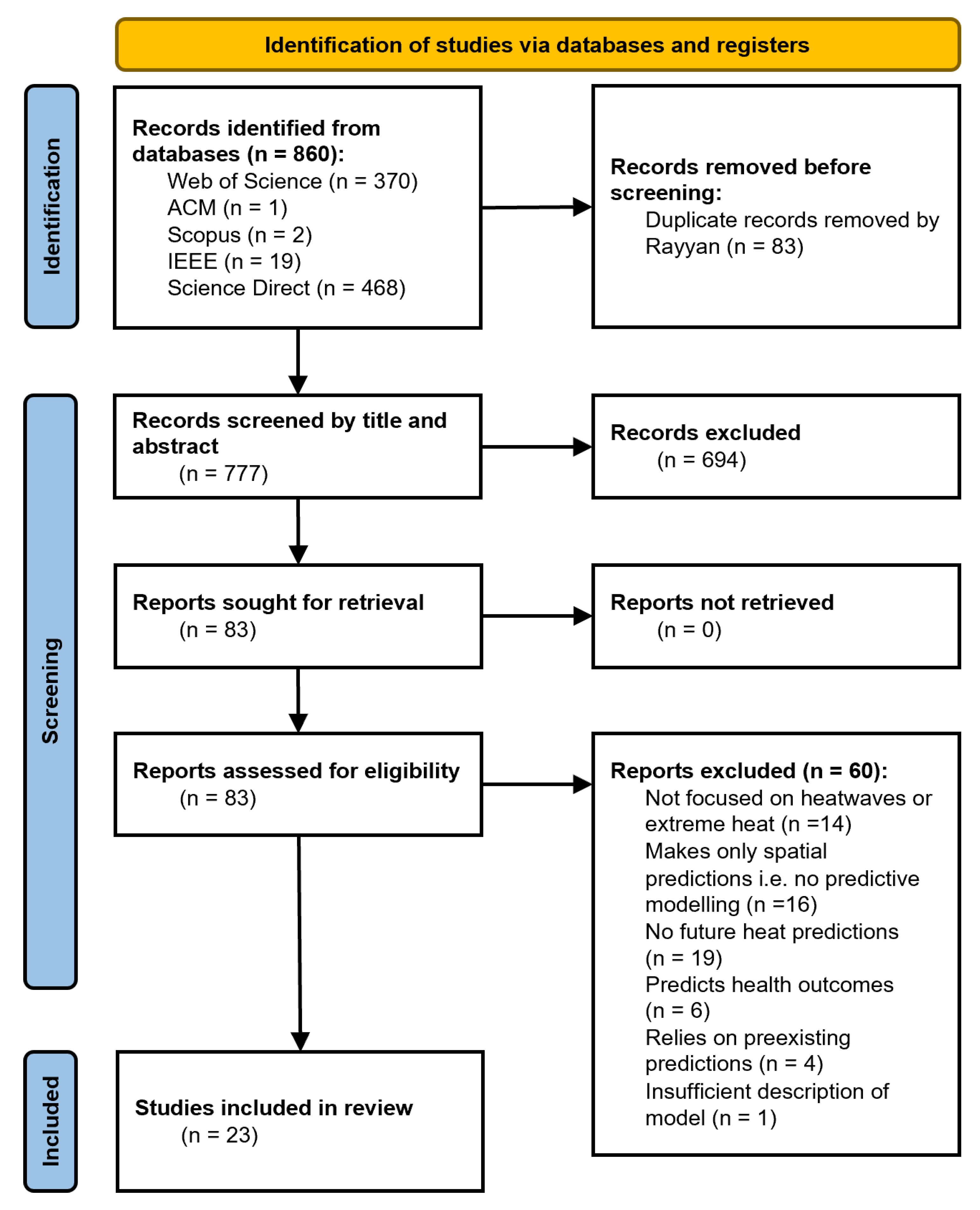
Figure 2.
World map illustrating the geographic distribution of the included studies by country. The largest number of studies was conducted in India (n = 4), followed by the USA (n = 3), Pakistan (n = 2), France (n = 2), and Spain (n = 2). One study each was reported from Bangladesh, Thailand, Taiwan, Italy, Japan, the United Kingdom, and Australia. Germany and Switzerland jointly contributed to one cross-national study; the total number of included studies remains n = 23.
Figure 2.
World map illustrating the geographic distribution of the included studies by country. The largest number of studies was conducted in India (n = 4), followed by the USA (n = 3), Pakistan (n = 2), France (n = 2), and Spain (n = 2). One study each was reported from Bangladesh, Thailand, Taiwan, Italy, Japan, the United Kingdom, and Australia. Germany and Switzerland jointly contributed to one cross-national study; the total number of included studies remains n = 23.
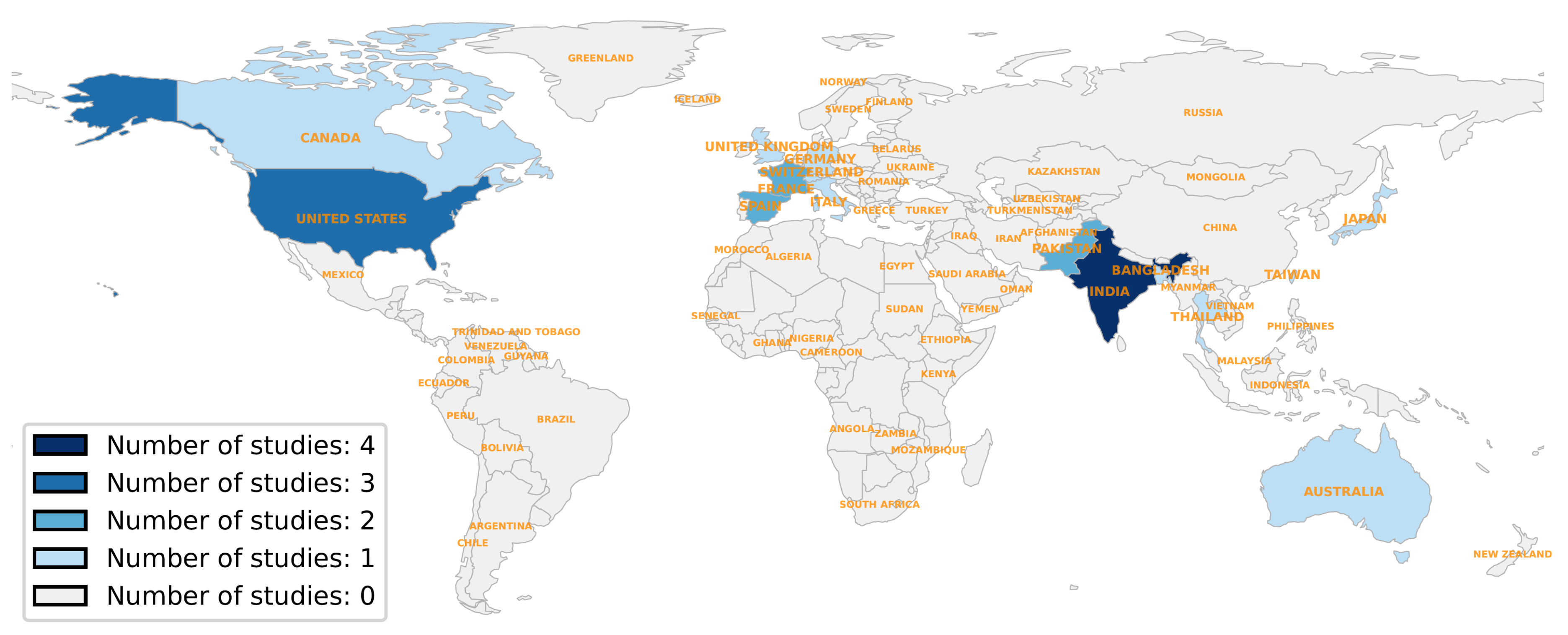
Figure 3.
Distribution of selected papers by year of publication and continent.
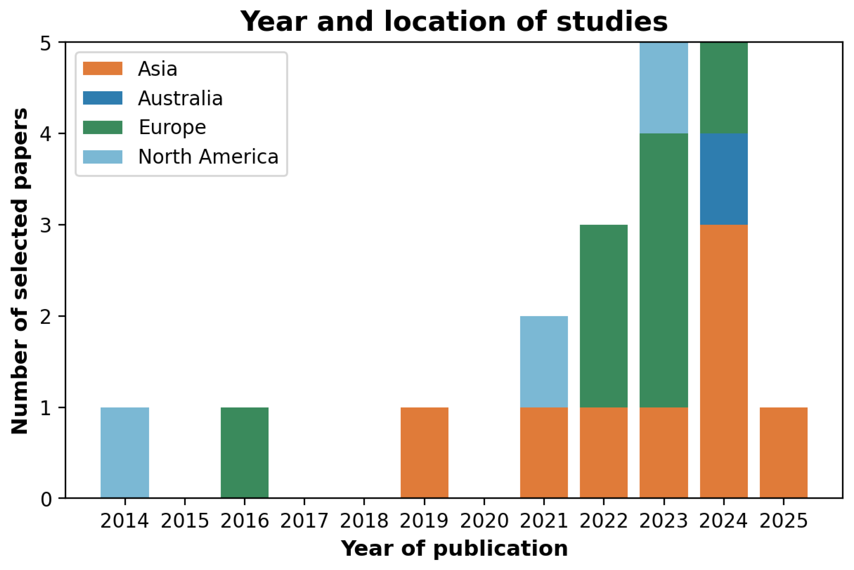
Figure 4.
Distribution of the types of heat-related risks or indicators predicted by the included studies.
Figure 4.
Distribution of the types of heat-related risks or indicators predicted by the included studies.
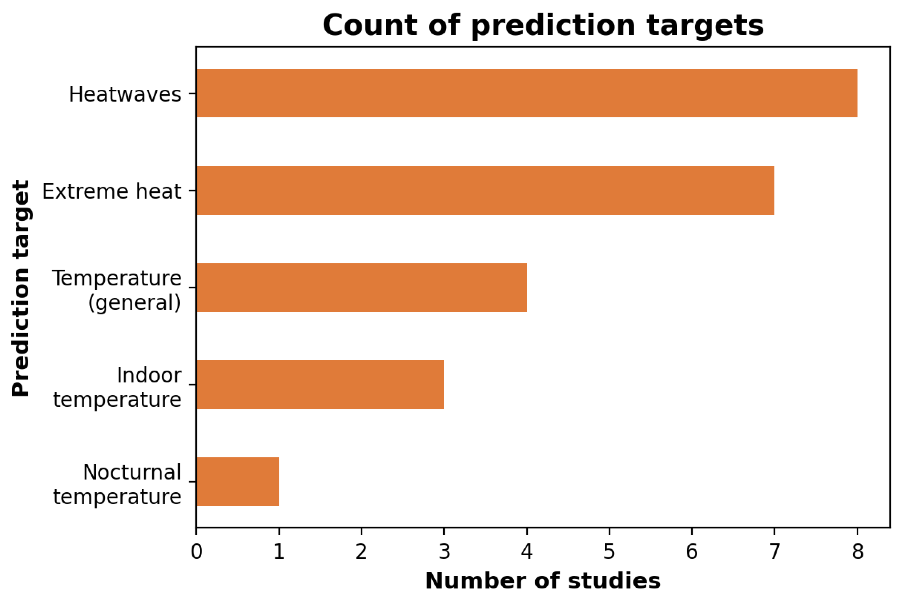
Figure 5.
Frequency of environmental predictors and derived features across included studies.
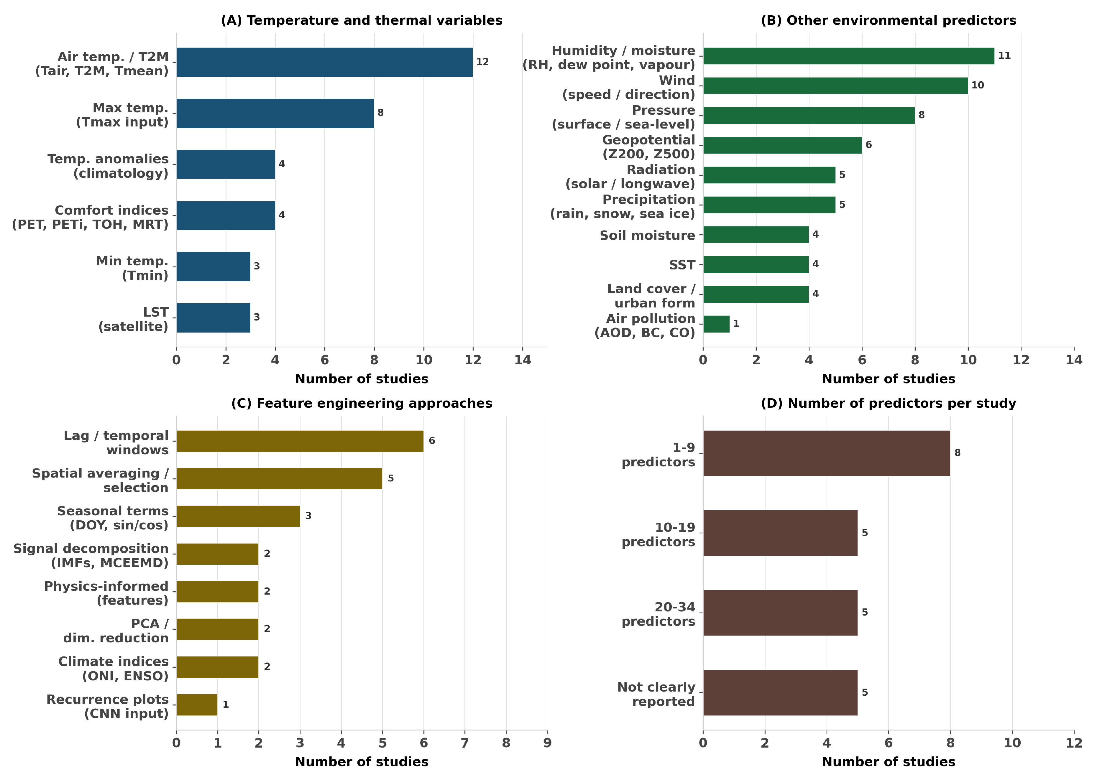
Figure 6.
ML Models and Performance metrics.
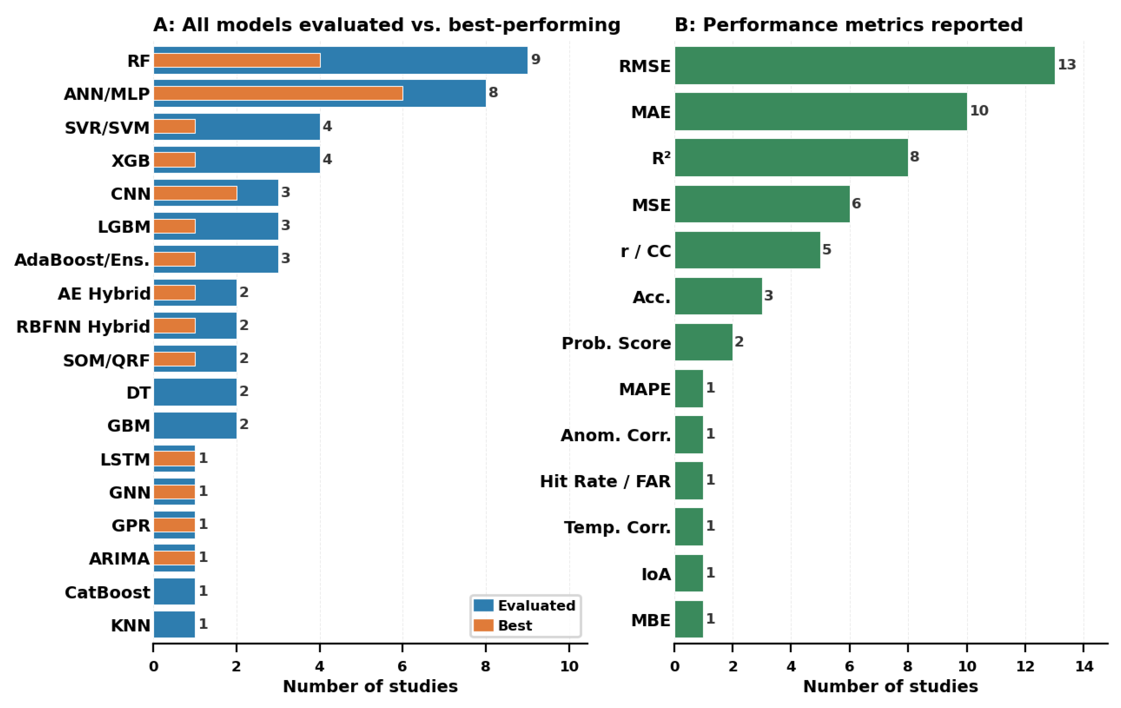
Table 2.
Summary of included studies on heatwave and extreme heat prediction using machine learning.
Table 2.
Summary of included studies on heatwave and extreme heat prediction using machine learning.
| Study (period) | Prediction target | Key predictors | Best model & Performance | Validation | Key finding |
|---|---|---|---|---|---|
| Ashtiani et al. (2014) [23] Summer 2010 | Indoor dry-bulb temp. during HW | Outdoor temp., solar radiation, wind, RH | ANN; RMSE = 1.76 °C | 70/15/15 split | ANN outperformed MLR (RMSE 1.76 vs. 2.10 °C); better captured nonlinear outdoor–indoor thermal interactions. |
| Bhoopathi et al. (2024) [24] 1991–2020 | Tmax; HW days at 7- and 15-day lead | Air temp., geopotential height, RH, soil moisture, SST | SVR: 7-day RMSE = 1.13 °C, 15-day RMSE = 1.20 °C | 70/30 temporal split | SVR is generally superior; accuracy declined in lower-temperature zones. |
| Carrión et al. (2021) [25] 2003–2019 | Hourly air temp. at 1-km resolution | MODIS LST, EVI, elevation, TPI, imperviousness | XGB; R2 ≈ 0.98, RMSE ≈ 1.5 K | Spatial 10-fold CV | XGB captured UHI patterns accurately; outperformed all statistical baselines and NLDAS-2. |
| Castro Medina et al. (2024) [26] 2022 | Urban air temperature distribution | Citizen-station temp. (current and lagged) | MLP; R2 = 0.98 | 50/50 temporal split | Citizen station networks with MLP accurately reproduced fine-scale urban temp. distributions. |
| Chaki et al. (2024) [27] 2011–2020 | Seasonal air temp. (May–Jul) | Air temp., RH, geopotential height, pressure, wind components | ANN (3 hidden layers); R2 = 0.20 | 80/20 split | Accuracy rose with more predictors; modest performance reflects Dhaka’s complex urban climate. |
| Chongtaku et al. (2024) [28] 1981–2019 | HW characteristics: HWN, HWF, HWD, HWM, HWA | Tmax, Tmin, MODIS LST (day/night) | RF (night LST); R2 = 0.64, RMSE = 2.09 °C | 80/20 split | Substantial urban–rural variability in HW characteristics; nighttime HW intensity highest in Bangkok. |
| Fister et al. (2023) [29] Historical | Seasonal summer temp.; extreme anomalies | Historical air temp. time series | RP+CNN; best ACC (values NR) | Multi-run MSE | RP+CNN outperformed classical ML; detected 2003 European HW anomaly. |
| Guhan et al. (2025) [30] 1980–2023 | Tmax, Tmin and rainfall forecasting | Tmax, Tmin, rainfall (IMD gridded) | ARIMA (Tmax; MAE = 3.01 °C); XGB (Tmin) | Comparative | Warming trends in Tmax/Tmin confirmed (1980–2023); ARIMA outperformed all ML models for Tmax. |
| Khan et al. (2022) [31] 1973–2017 | HW occurrence (binary) | Tmax, humidity, precipitation, wind, pressure | RF; ACC ≈ 0.91 | Temporal split | RF most effectively predicted HW occurrence; Tmax was the dominant predictor. |
| Li et al. (2023) [32] 2006–2020 | HW occurrence (binary) | Tmax, Tmin, dew point, pressure, precipitation, wind, ONI | GNN; ACC = 94.1%, Recall = 58.5% | Temporal split | GNN captured spatiotemporal station interactions; ONI improved concurrent multi-station HW prediction. |
| Lin et al. (2021) [33] 1960–2017 | Daily Tmax up to 7 days ahead | Lagged Tmax (prior 7 days) | MCEEMD-RBFNN; R = 0.75–0.94, RMSE ≈ 0.9–1.7 °C | 80/20 temporal split | Signal decomposition before NN training substantially improved short-range Tmax forecasting. |
| Miloshevich et al. (2023) [34] 8,000-yr sim. | Extreme HW occurrence (probabilistic) | Z500, 2-m temp. | CNN (probabilistic); positive skill to ∼15 days | Stratified 10-fold CV | Z500 and soil moisture dominated; 2-m temp. added negligible skill once these were included. |
| Oliveira et al. (2022) [35] 2000–2020 | Nocturnal LST; Surface Urban Heat Island intensity | Altitude, Longitude, Latitude, Nocturnal LST (satellite imagery), Heat flux | RF; MSE < 1°K, R2 = 0.95 | Train/test split (70/30) | Latent and storage heat flux are the most important non-spatial predictors; the use of satellite imagery allows the construction of sub-1km data. |
| Perez Aracil et al. (2024) [36] 1950–2022 | 2-m air temp. at 1–4 weeks ahead | SST, Z500, MSL, wind components, T2M | AE*+MLP; best across most cities and horizons | Temporal LOYO | Autoencoder hybrids improved sub-seasonal temp. prediction across 7 EU cities; coastal sites more stable. |
| Polasky et al. (2022) [37] Hist. + future | Downscaled temp., precip., dew point | Synoptic atmospheric patterns | Statistical downscaling; PDF skill ≈ 1 | PDF vs. obs. | Distribution-based evaluation better captured extremes; improved tail temperature representation. |
| Ratnam et al. (2023) [38] 1982–2020 | Tmax anomalies 10 days ahead (Mar–Jun) | SST (North Atlantic, ENSO-related), soil moisture, Z200 | AdaBoost(MLP); ACC = 0.33–0.46 | LOYO CV; vs. CFSv2 | AdaBoost(MLP) outperformed all 9 other models; skill comparable to CFSv2 in April–May. |
| Reddy et al. (2024) [39] 2009, 2019 events | WRF heat extreme variables (temp., RH, wind) | 24 WRF physics parameters (P14, P17, P22 most influential) | GPR surrogate; high R2 (values NR) | 8-fold CV | Only 3 of 24 WRF parameters significantly influenced heat outputs; GPR reduced sensitivity analysis cost. |
| Shafiq et al. (2025) [40] 2018–2022 | Extreme heat event occurrence (binary, 1–3 day lead) | Tmax, Tmin, humidity, pressure, wind | LSTM; ACC = 96.2% | 80/20; early stopping | LSTM achieved highest ACC; SHAP and LIME confirmed humidity and Tmax as dominant predictors. |
| Sulzer et al. (2023) [41] 2021–2022 | Indoor air temp. and PET up to 24 h ahead | Outdoor temp., vapour pressure, MSLP, solar & LW radiation | ANN; MAETi = 0.87 K; Corr = 0.98 | Train/val/test; early stopping | ANN with indoor sensors and NWP outperformed outdoor-only models; 91% of forecasts within 2 K. |
| Suthar et al. (2023) [42] 2013–2022 | Tmax for HW identification (IMD criteria) | LST, AOD, black carbon, CO, BLH, TCWV, RH | RF; adj. R2 = 0.90–0.92 | 3-fold CV | RF accurately predicted Tmax from satellite inputs; LST and black carbon were the strongest predictors. |
| Symonds et al. (2016) [43] Present + 2050 | Indoor overheating risk (TOH), air pollution, energy use | Outdoor temp., humidity, PM2.5, building and occupancy variables | ANN; R2 = 0.89–0.92 | 500/100 sim. split | ANN emulated EnergyPlus simulations for rapid national-scale indoor overheating risk estimation. |
| Xie et al. (2022) [44] 2014–2019 | MRT distribution around buildings | Air temp., solar radiation, building geometry, urban morphology | MLNN-GA-BP; high ACC (values NR) | Temporal holdout (2019) | GA-optimised ANN predicted spatial MRT distributions; supports outdoor thermal comfort assessment on hot days. |
| Zhang et al. (2022) [45] 1981–2020 | Summer HWF | SST, soil moisture, snow cover, sea ice | LightGBM; TCC = 0.36 | 5-fold CV; hindcast | LightGBM outperformed MLR; SST contributed ∼70% of predictive skill; preceding winter conditions were critical. |
Notes: Full domain-level detail is provided in Supplementary File S1. Abbreviations: ACC: Accuracy; AE: Autoencoder; ANN: Artificial Neural Network; ARIMA: Autoregressive Integrated Moving Average; AOD: Aerosol Optical Depth; BLH: Boundary Layer Height; CO: Carbon Monoxide; CNN: Convolutional Neural Network; Corr: Correlation coefficient; CV: Cross-Validation; EVI: Enhanced Vegetation Index; GA: Genetic Algorithm; GNN: Graph Neural Network; GPR: Gaussian Process Regression; HW: Heatwave; HWA/D/F/M/N: HW amplitude/duration/frequency/magnitude/number; IMD: India Meteorological Department; LOYO: Leave-One-Year-Out; LST: Land Surface Temperature; LW: Longwave; LSTM: Long Short-Term Memory; MAE: Mean Absolute Error; MCEEMD: Multi-dim. Complementary EEMD; MLP: Multilayer Perceptron; MLNN: Multilayer NN; MLR: Multiple Linear Regression; MRT: Mean Radiant Temperature; MSL/MSLP: Mean Sea-Level Pressure; NR: Not Reported; NWP: Numerical Weather Prediction; obs.: observations; ONI: Oceanic Niño Index; PDF: Probability Density Function; PET: Physiologically Equivalent Temperature; RBFNN: Radial Basis Function NN; RF: Random Forest; RH: Relative Humidity; RMSE: Root Mean Square Error; RP: Recurrence Plot; SHAP: Shapley Additive Explanations; sim.: simulation; SST: Sea Surface Temperature; SVM: Support Vector Machine; SVR: Support Vector Regression; TCWV: Total Column Water Vapour; TCC: Temporal Correlation Coefficient; TOH: Temperature Overheating metric; TPI: Topographic Position Index; Tmax/Tmin: Max/Min Temperature; UHI: Urban Heat Island; XGB: Extreme Gradient Boosting; Z200/Z500: 200/500 hPa Geopotential Height.
Disclaimer/Publisher’s Note: The statements, opinions and data contained in all publications are solely those of the individual author(s) and contributor(s) and not of MDPI and/or the editor(s). MDPI and/or the editor(s) disclaim responsibility for any injury to people or property resulting from any ideas, methods, instructions or products referred to in the content. |
© 2026 by the authors. Licensee MDPI, Basel, Switzerland. This article is an open access article distributed under the terms and conditions of the Creative Commons Attribution (CC BY) license (http://creativecommons.org/licenses/by/4.0/).
Copyright: This open access article is published under a Creative Commons CC BY 4.0 license, which permit the free download, distribution, and reuse, provided that the author and preprint are cited in any reuse.


