

Submitted:
09 September 2026
Posted:
11 September 2026
You are already at the latest version
Abstract
Accurate dimensional and deformation measurement of mechanical components is central to manufacturing quality control and experimental mechanics. Contact-based instruments such as Vernier calipers, micrometers, and coordinate measuring machines (CMMs) are widely used but introduce measurement loading and cannot simultaneously capture multi-point displacements. Commercial optical alternatives, such as Vic-2D and GOM Aramis for Digital Image Correlation (DIC) and HALCON for machine vision, provide high accuracy but carry license costs that restrict adoption in academic laboratories and small engineering workshops. This review examines two freely available, open-source platforms that together provide comprehensive non-contact 2D measurement of planar mechanical components: Python OpenCV, which enables camera calibration, homography-based planar reconstruction, adaptive Gaussian thresholding for metallic surfaces, and sub-pixel edge detection; and MATLAB NCORR, an open-source Digital Image Correlation (DIC) package that computes full-field displacement and strain maps from random speckle patterns. The review is directed at general planar mechanical components as: flat rectangular parts, cylindrical fasteners, threaded screws, gears, and beam specimens.Experimental results obtained using a mobile phone camera and the Python-OpenCV pipeline demonstrate dimensional measurement errors below 1.5% relative to Vernier caliper measurements for a flat rectangular component (scientific calculator) and below 1% for length and outer diameter of a metallic machine screw, confirming sub-millimetre accuracy for components in the 10–200 mm size range. Thread pitch measurement via horizontal edge projection is reported as a specific limitation at standard mobile phone image magnification, with error exceeding 89%, and a Hough Transform solution is proposed. An integrated two-tool workflow combining OpenCV discrete-point tracking with NCORR full-field DIC strain mapping is proposed for comprehensive mechanical component characterization at near-zero software cost.
Keywords:
machine vision
; Python
; OpenCV
; MATLAB
; NCORR
; digital image correlation
; DIC
; dimensional measurement
; strain measurement
; adaptive gaussian thresholding
; open-source metrology
; non-contact measurement
1. Introduction
Dimensional and deformation measurement of mechanical components underpins manufacturing inspection, experimental mechanics, and product validation. Traditional contact instruments such as Vernier calipers, micrometers, dial gauges, and CMM touch probes are reliable for rigid components but have three practical limitations. First, the instrument contacts the specimen, applying a probing force that can deform flexible or miniaturized components. Second, each sensor measures one point at a time, making it impossible to capture simultaneously correlated multi-point displacements. Third, high-accuracy CMMs cost significantly more than mobile optical alternatives, restricting access in academic and small-industry settings.
Non-contact optical measurement using cameras and image processing avoids all three limitations. A calibrated camera captures all visible surface points simultaneously in each frame without applying any mechanical load. With appropriate sub-pixel algorithms, dimensional accuracy in the sub-millimetre range is achievable with commercially available mobile phone cameras and free software [1,2]. Despite these advantages, commercial vision measurement and DIC software (HALCON, Vic-2D, GOM Aramis) carry per-seat license costs that limit their use in teaching laboratories and small engineering workshops.
Two freely available open-source platforms remove this barrier. Python OpenCV [3] is a cross-platform computer vision library providing calibration, homography, optical flow, and sub-pixel edge detection; all required for a complete 2D planar measurement pipeline — at zero cost. MATLAB NCORR [4] is an open-source Digital Image Correlation package that computes full-field displacement and strain maps from speckle-pattern images with accuracy comparable to commercial DIC platforms.
This paper complements the authors’ companion review published in Micromachines [5], which examined 2D vision measurement specifically for a Single-Input Dual-Output Compliant Displacement Amplification Mechanism (SIDO-CDAM) [6]. The present paper restricts its scope to general planar mechanical components such as, flat rectangular parts, cylindrical fasteners, threaded screws, gears, and standard beam specimens; which represent the far more common measurement targets in undergraduate laboratories, workshop inspection, and industrial quality control. The paper makes five contributions: (i) a focused review of Python OpenCV for 2D dimensional and displacement measurement; (ii) a review of MATLAB NCORR for full-field DIC strain measurement; (iii) experimental validation of the OpenCV pipeline on two component types using a mobile phone camera, with quantitative accuracy data; (iv) documentation of the thread pitch measurement limitation at standard mobile phone magnification and a proposed Hough Transform solution; and (v) proposal of an integrated two-tool measurement workflow for general mechanical components.
2. Python OpenCV for 2D Dimensional and Displacement Measurement
2.1. Overview
OpenCV (Open Source Computer Vision Library) [3] is a BSD-licensed, cross-platform library providing over 2,500 optimized algorithms for image processing and computer vision. Freely installable via the Python package manager (pip install opencv-python), it provides camera calibration [7], homography-based world-plane reconstruction, Lucas-Kanade pyramidal optical flow tracking [8], and sub-pixel edge localization: all required for a complete 2D measurement pipeline at no software cost. It is used in peer-reviewed academic measurement studies [1,2,9] and industrial inspection applications [10,11]
2.2. Camera Calibration
Camera calibration estimates the intrinsic parameters — focal length, principal point, and lens distortion coefficients — and extrinsic parameters (rotation and translation between camera and world frames). Zhang’s checkerboard method [7], implemented in OpenCV as cv2.calibrateCamera(), recovers these from 15–25 images of a printed checkerboard captured from different orientations. Distortion correction is important for measurements spanning the full image field: uncorrected radial distortion can introduce positional errors at the image periphery that reduce dimensional accuracy. A reprojection error below 0.5 pixels is recommended for workshop-level inspection accuracy.
For practical laboratory use where the camera-to-specimen distance changes between sessions a scale-factor calibration provides a simpler starting point. A scale-factor calibration is computing a pixel-to-millimetre conversion factor from one reference object of known size. This approach was used in the experimental validation reported in Section 4. For higher accuracy, ArUco fiducial markers [3] of precisely known size placed alongside the specimen in each image allow automatic per-image scale-factor computation without a separate calibration session. Arellano-González et al. [9] compared homogeneous and non-homogeneous DLT calibration methods and confirmed reliable trajectory tracking for planar mechanisms with low-cost hardware.
2.3. Homography-Based Planar Reconstruction
A homography matrix H (3×3, 8 degrees of freedom) maps image-plane pixel coordinates to world-plane physical coordinates:
s · [u, v, 1]ᵀ = H · [X, Y, 1]ᵀ
Unlike a fixed pixel-to-millimetre scale factor, homography compensates for perspective distortion and magnification non-uniformity across the image. Wu et al. [1] demonstrated that SVD decomposition of H recovers translational and rotational motion components with higher accuracy and repeatability than scale-factor methods on a robotic stage. For mobile phone cameras, which typically have some barrel distortion and perspective variation across the field; homography-based back-projection is more robust than a fixed scale factor, particularly for components spanning a significant fraction of the image field.
2.4. Camera Motion Compensation
Any movement of the mobile phone camera between image captures — vibration, accidental nudging, thermal drift — appears as false displacement in the measurement. Jiao et al. [12] proposed placing fixed reference markers on the stationary surface adjacent to the specimen; the apparent motion of these markers per frame represents unintentional camera motion, which is subtracted from all tracked feature positions. This compensation requires no additional hardware and is particularly relevant for mobile phone measurements where the camera is handheld or loosely mounted.
2.5. Adaptive Gaussian Thresholding for Metallic Components
Converting the greyscale image to a binary (object/background) image for contour extraction is a critical preprocessing step. Global thresholding (Otsu’s method) works well for uniform-coloured specimens but fails for metallic components — machine screws, bolts, machined aluminium parts — where semi-specular surfaces produce locally varying brightness under standard room lighting. Bright specular reflections and dark thread valleys can both be incorrectly classified, producing a fragmented or incorrect silhouette.
Adaptive Gaussian Thresholding (cv2.adaptiveThreshold() with ADAPTIVE_THRESH_GAUSSIAN_C) computes a different threshold for each local pixel neighbourhood (typically block size 11, constant C = 2) based on the Gaussian-weighted average of surrounding pixels. This local adaptation handles large-scale brightness non-uniformity reliably, producing clean closed silhouettes of metallic components under standard room lighting — conditions typical of a mobile phone measurement setup. A morphological closing operation (3×3 kernel, two iterations) applied after thresholding fills residual gaps in the binary outline caused by thread root shadowing.
2.6. Geometry Fitting for Dimensional Extraction
After contour detection (cv2.findContours()), two bounding constructs extract dimensions from the largest contour. The axis-aligned bounding rectangle (AABR, cv2.boundingRect()) defines the region for thread analysis. The minimum area rotated rectangle (MARR, cv2.minAreaRect()) fits the smallest enclosing rectangle at any angle, providing orientation-independent length and diameter: the larger dimension equals total length and the smaller equals outer diameter, regardless of component orientation in the image. Thread length is estimated from the AABR of the threaded zone; thread pitch is estimated via horizontal edge projection over the threaded region.
2.7. Sub-Pixel Edge Detection
Sub-pixel edge detection improves dimensional accuracy beyond the native pixel resolution. Xie et al. [11] proposed a two-stage hybrid: Roberts operator for coarse pixel-level edge detection followed by improved Zernike moment fitting for sub-pixel refinement, with Otsu’s method for automatic threshold selection. This combination achieves better accuracy and lower computational cost than pure Zernike methods and is particularly suited to straight or mildly curved edges typical of machined components. Cheng et al. [13] demonstrated 3 µm accuracy on shaft parts using Canny detection with Hessian-matrix sub-pixel localisation (Canny-Steger method). For mobile phone measurements at mm-level accuracy, standard sub-pixel refinement through cv2.cornerSubPix() is sufficient, achieving localization to within 0.1–0.2 pixels.
2.8. Accuracy at Mobile Phone Resolution
Table 1 summarizes expected dimensional accuracy for different optical configurations. At mobile phone magnification (PIXEL_TO_MM ≈ 0.05 mm/pixel for a 30 cm working distance), sub-pixel precision of 0.1–0.2 pixels translates to 0.005–0.010 mm absolute pixel-level resolution. However, additional contributions from scale-factor calibration error, perspective distortion, and lighting non-uniformity bring the practical measurement uncertainty to the sub-millimetre range — confirmed by the experimental results in Section 4.
3. MATLAB NCORR for Full-Field DIC Displacement and Strain Measurement
3.1. DIC Principle
Digital Image Correlation (DIC) [15] is a non-contact, full-field technique that quantifies deformation by tracking a random speckle pattern applied to the specimen surface. A reference image (unloaded state) is compared with deformed images to recover the displacement field u(x, y) = [u, v] by minimising the Zero-Normalized Cross-Correlation (ZNCC) criterion:
where f and g are the normalized intensity distributions of the reference and deformed subsets. NCORR [4] refines an initial integer-pixel displacement estimate using an iterative Levenberg-Marquardt solver, achieving 0.01–0.05 pixel displacement accuracy. Its Reliable Filtering Algorithm (RFA) computes a quality metric per pixel and masks unreliable regions such as low-texture zones, occluded areas, crack edges which preventing poor correlation data from contaminating the displacement field [4]. NCORR is freely available at https://github.com/justinblaber/ncorr_2D_matlab, runs in MATLAB R2012b and later (including student edition), requires no toolboxes, and provides both a GUI and scriptable API.
3.2. Speckle Pattern Preparation
DIC requires the specimen surface within the region of interest (ROI) to carry a random, isotropic, high-contrast speckle pattern with speckle size of 3–7 pixels in the acquired image. Speckles smaller than 2–3 pixels cause correlation noise; speckles larger than 7–10 pixels reduce the spatial resolution of the strain field [15,16]. Table 2 summarizes recommended preparation methods by component scale.
3.3. NCORR Processing Workflow
The NCORR pipeline comprises five steps: (i) loading the reference and deformed image sequence; (ii) drawing the ROI over the specimen area of interest; (iii) setting correlation parameters — subset radius r (15–25 pixels), strain radius e (10–15 pixels), step size s (1–5 pixels); (iv) executing the correlation analysis with Levenberg-Marquardt sub-pixel refinement; and (v) computing strain fields by local polynomial fitting — more noise-robust than finite differencing. Figure 1 illustrates the NCORR workflow on a representative mechanical component.
revealing stress concentration. The same workflow applies to flat parts, fasteners, gears, and beams.
3.4. Strain and Stress Computation
From displacement fields u(x,y) and v(x,y), NCORR computes strain components , , using the linearized small-strain approximation for elastic engineering applications. For isotropic linear elastic materials under plane stress:
The Von Mises stress identifies the location and magnitude of maximum stress concentration, comparable to FEA predictions. For steel (E = 200 GPa, ν = 0.30) and aluminium (E = 70 GPa, ν = 0.33), stress fields are computed directly from NCORR-exported strain matrices using standard material constants.
3.5. Accuracy and Comparison with Commercial DIC
Table 3 compares NCORR with representative commercial DIC platforms and the emerging Python-based iCorrVision-2D.
4. Experimental Validation on Standard Mechanical Components
4.1. Experimental Setup
To validate the OpenCV pipeline, experiments were conducted on two standard mechanical component types using readily available laboratory equipment. A 12 MP mobile phone camera (f/1.8 aperture) was positioned approximately 25–30 cm above the specimen, perpendicular to a white A4 paper background, under diffuse room lighting. A scale-factor calibration of PIXEL_TO_MM = 0.05 mm/pixel was established from a reference object of known dimensions. Images were standardized to 700 × 1000 pixels before processing.
The processing pipeline applied to each specimen was: (1) grayscale conversion; (2) Gaussian blur (5 × 5 kernel, σ = 0); (3) adaptive Gaussian thresholding (block size 11, C = 2); (4) morphological closing (3 × 3 kernel, two iterations); (5) largest-contour selection (minimum area 3,000 px²); (6) MARR fitting for total length and outer diameter; (7) AABR-based thread zone extraction; (8) horizontal edge projection for thread pitch; (9) calibration conversion and annotated output display. Figure 2 illustrates the complete pipeline.
4.2. Phase I: Flat Rectangular Component
A scientific calculator was selected as a representative flat rectangular component with a well-defined outline and known nominal dimensions, verified by Vernier caliper measurement (length = 162.00 mm, width = 77.00 mm). Flat rectangular components represent the simplest and most common inspection target: injection-moulded housings, sheet metal brackets, PCB outlines, and flat plates. Table 4 reports the measurement results.
All parameters were within 1.4% of the Vernier reference, confirming that the adaptive thresholding and MARR pipeline functions correctly for flat rectangular components. Absolute errors of 0.60 mm (length) and 0.80 mm (width) are consistent with the expected sub-millimetre accuracy of a mobile phone measurement at 0.05 mm/pixel pixel pitch. Figure 3 shows the annotated output.
4.3. Phase II: Threaded Cylindrical Fastener
A stepped metallic machine screw — with a smooth cylindrical shank section and an external V-thread section — was selected as a representative threaded cylindrical fastener. This is a more demanding specimen than the flat component because: (i) the metallic surface is semi-specular under room lighting; (ii) the geometry combines multiple features (total length, outer diameter, thread length, thread pitch); and (iii) the thread profile produces an irregular silhouette. Adaptive Gaussian thresholding successfully produced a clean, closed silhouette where global Otsu thresholding failed. Table 5 reports the results.
Total length and outer diameter were both measured within 1% of Vernier references — absolute errors of 0.25 mm and 0.10 mm respectively. Thread length agreed within 2.73%. These results confirm that the adaptive thresholding and MARR pipeline extends reliably to metallic cylindrical components. Figure 4 shows the annotated output.
4.4. Thread Pitch Measurement — Documented Limitation and Solution
The horizontal edge projection method returned a measured thread pitch of 0.16 mm against the M10 standard pitch of 1.50 mm with an error exceeding 89%. This is a resolution-dependent limitation, not a system failure, and it applies to any camera-projection system where image magnification is insufficient to resolve thread crests as distinct peaks.
Explanation. At PIXEL_TO_MM = 0.05 mm/pixel, the M10 pitch of 1.50 mm spans 1.50/0.05 = 30 pixels. In principle, peaks in the horizontal edge projection should appear every 30 pixels. In practice, each thread crest generates multiple edge pixels at the leading flank, crest flat, and trailing flank. The peak-detection algorithm finds local maxima between individual sub-feature edge clusters — spaced approximately 0.16 mm / 0.05 = 3.2 pixels apart — rather than between thread crests.
Solution: Hough Line Transform. Applying the Hough Line Transform (cv2.HoughLines()) to the Canny edge image over the thread zone detects the inclined lines formed by thread flanks, which appear as parallel diagonals at the thread helix angle α. Thread pitch is then computed as p = πd·tan(α), where d is the mean thread diameter from MARR. This approach is independent of image magnification and is expected to reduce thread pitch error to below 10% at standard mobile phone magnification.
General design rule. For the horizontal projection method to distinguish thread crests: crest spacing ≥ 30 pixels is required. This translates to a minimum magnification of 30/(pitch in mm) pixels/mm. For M10 (1.50 mm pitch): ≥ 20 px/mm; for M6 (1.00 mm): ≥ 30 px/mm; for M4 (0.70 mm): ≥ 43 px/mm. At 0.05 mm/pixel (20 px/mm), only threads with pitch ≥ 1.50 mm are theoretically measurable by the projection method — the M10 is at this limit, meaning the Hough Transform approach is strongly recommended.
5. Benchmarking Against Contact Instruments and Commercial Alternatives
5.1. Measurement Method Comparison
Table 6 summarises the comparative assessment of OpenCV, NCORR, and conventional measurement instruments for general planar mechanical components.
5.2. Complementarity of OpenCV and NCORR
OpenCV tracks discrete named points and edges — two ends of a deflecting beam, the output ports of a compliant mechanism, corner marks of a bracket — providing direct dimensional or displacement readings. NCORR measures how the entire specimen surface deforms — strain distribution, stress concentration zones, crack fronts — simultaneously at every pixel. Neither tool provides the output of the other. For comprehensive characterization, both tools can be applied to the same image sequence using a single camera: fiducial markers at named measurement points for OpenCV tracking, and a random speckle pattern on the specimen body for NCORR DIC. This requires one camera, one lighting setup, and one acquisition session.
5.3. Economic Assessment
The experimental validation in Section 4 was conducted using a mobile phone and a laptop at zero additional hardware cost, confirming sub-millimetre accuracy for standard mm-scale components. This places the approach within reach of: (i) undergraduate mechanical engineering laboratories with no vision measurement budget; (ii) small engineering workshops where a CMM is unaffordable; and (iii) field inspection scenarios where a portable, non-contact measurement is needed. The software (Python + OpenCV + MATLAB NCORR) is entirely free. For users without MATLAB, the Python-based iCorrVision-2D [18] provides a free alternative for DIC, though with more limited validation.
6. Applications, Limitations, and Research Gaps
6.1. Applications by Component Type
Flat rectangular and polygonal parts. Camera calibration + MARR fitting (Section 2.6) extracts length, width, and projected area. Phase I results confirm < 1.5% error for a 162 mm × 77 mm component at mobile phone resolution. Applications include injection-moulded part outline inspection, flat bracket verification, and PCB outline measurement.
Cylindrical and threaded fasteners. Adaptive Gaussian thresholding + MARR reliably extracts total length and outer diameter within 1% for metallic screws and bolts at mobile phone resolution. Thread length is recoverable within 3%. Thread pitch requires the Hough Transform approach described in Section 4.4 for accuracy below 10%.
Gears and toothed components. Duan et al. [19] demonstrated 1.9 µm maximum error using Gaussian integral sub-pixel detection on gear tooth profiles. Moru and Borro [10] demonstrated gear inspection at ±0.020 mm tolerance validated against CMM. The OpenCV calibration and contour extraction pipeline of Section 2 integrates directly with these sub-pixel gear tooth methods.
Tensile and bending test specimens. NCORR was developed and validated on tensile specimens [4] and provides full-field , , maps. NCORR strain accuracy within ±100 µε compared to calibrated extensometers is confirmed for metallic specimens [19]. OpenCV complements NCORR for extensometry: tracking two gauge marks provides gauge-length elongation independently verifiable against the DIC-integrated strain.
Structural members and joints. Jiao et al. [12] demonstrated sub-pixel displacement measurement of structural members under loading with camera motion correction. Xu and Brownjohn [20] reviewed vision-based displacement measurement for civil structures. These approaches apply directly to laboratory beam bending, frame tests, and welded joint inspection using the OpenCV pipeline of Section 2.
6.2. Limitations
- Thread pitch accuracy at mobile phone magnification: The horizontal projection method gives >89% error for M10 threads at 0.05 mm/pixel. The Hough Transform approach (Section 4.4) resolves this.
- Scale-factor calibration is session-fixed: The PIXEL_TO_MM constant must be re-established when camera distance changes. ArUco per-image automatic calibration eliminates this limitation.
- OpenCV measures discrete points only: Full-field strain maps require NCORR DIC. An integrated session (OpenCV + NCORR on the same images) is recommended for complete characterization.
- NCORR requires MATLAB: MATLAB carries a license cost for non-academic users. iCorrVision-2D [18] is a Python-based free alternative with growing validation support.
- Lighting sensitivity: Mobile phone ambient room lighting produces non-uniform illumination. Adaptive thresholding mitigates this for binary segmentation; a dedicated LED ring light improves reliability and is recommended for regular inspection use.
6.3. Research Gaps
Table 7 identifies five research gaps derived from this review.
7. Conclusions
This paper reviewed two freely available open-source platforms: Python OpenCV and MATLAB NCORR — for non-contact 2D measurement of general planar mechanical components, including flat parts, cylindrical fasteners, gears, and beam specimens. The following conclusions are drawn.
- Python OpenCV with a mobile phone camera achieves sub-millimetre dimensional accuracy for standard mm-scale components. Using adaptive Gaussian thresholding for metallic surfaces, MARR fitting for orientation-independent extraction, and scale-factor calibration, the framework achieves < 1.5% dimensional error (absolute errors of 0.10–0.80 mm) for components in the 10–200 mm size range under standard room lighting — confirming suitability for workshop inspection at zero software cost.
- Adaptive Gaussian Thresholding is essential for metallic components under room lighting. Global (Otsu) thresholding fails to produce reliable contours on semi-specular metallic surfaces. Adaptive Gaussian Thresholding, with block size 11 and constant C = 2, reliably produces clean closed contours on metallic fasteners under diffuse room lighting — the standard condition for mobile phone measurements.
- Thread pitch measurement via horizontal edge projection is resolution-limited at mobile phone magnification. An error exceeding 89% is documented for M10 thread pitch at 0.05 mm/pixel. The Hough Line Transform on thread flank angles is proposed as the correct solution, together with a design rule: crest spacing ≥ 30 pixels is required for reliable projection peak detection.
- MATLAB NCORR provides full-field strain measurement comparable to commercial DIC at zero software cost. With 50–200 µε strain accuracy and over 500 validated publications, NCORR complements OpenCV dimensional tracking by providing the strain distribution across the entire specimen surface — identifying stress concentration zones and enabling point-by-point FEA comparison.
- OpenCV and NCORR are complementary tools best used together. An integrated single-session workflow — fiducial markers at named points for OpenCV, speckle pattern on the specimen body for NCORR — provides comprehensive non-contact dimensional and strain characterization using one camera and one image acquisition sequence, at near-zero total software cost.
Author Contributions
Conceptualization: R.R.O.; Methodology: R.R.O., K.V.P.; Investigation: K.V.P., T.K.G., S.M.B., G.S.C.; Literature review: K.V.P., T.K.G., S.M.B., G.S.C.; Writing — original draft: R.R.O., K.V.P.; Writing — review and editing: R.R.O.; Supervision: R.R.O. All authors have read and agreed to the published version of the manuscript.
Funding
This research received no external funding.
Data Availability Statement
No new datasets beyond those reported in Table 4 and Table 5 are created in this study. MATLAB NCORR is freely available at https://github.com/justinblaber/ncorr_2D_matlab. Python OpenCV is available at https://pypi.org/project/opencv-python/.
Acknowledgments
The authors acknowledge the use of Consensus AI (consensus.app) for structured academic literature search during the preparation of this review. All papers were independently verified for quality and relevance before inclusion.
Conflicts of Interest
The authors declare no conflict of interest.
Abbreviations
The following abbreviations are used in this manuscript:
| AABR | Axis-Aligned Bounding Rectangle |
| ArUco | Augmented Reality University of Córdoba (fiducial marker system) |
| CMM | Coordinate Measuring Machine |
| DIC | Digital Image Correlation |
| DOF | Degrees of Freedom |
| ESM | Efficient Second-order Minimization |
| FEA | Finite Element Analysis |
| MARR | Minimum Area Rotated Rectangle |
| NCORR | Open-source MATLAB DIC package (Blaber et al., 2015) |
| OpenCV | Open Source Computer Vision Library |
| PIXEL_TO_MM | Pixel-to-millimetre scale calibration factor |
| RANSAC | Random Sample Consensus |
| RFA | Reliable Filtering Algorithm (NCORR) |
| ROI | Region of Interest |
| SIDO-CDAM | Single-Input Dual-Output Compliant Displacement Amplification Mechanism |
| ZNCC | Zero-Normalized Cross-Correlation |
| µε | Microstrain (10⁻⁶ m/m) |
References
- Wu, L.; Deng, X.; Wang, Y.; Du, X.; Xiong, X.; Jiang, B. Research on Vision-Based Robot Planar Motion Measurement Method. J. Braz. Soc. Mech. Sci. Eng. 2023, 45, 216. [Google Scholar] [CrossRef]
- Nogueira, V.V.E.; Barca, L.F.; Pimenta, T.C. A Cost-Effective Method for Automatically Measuring Mechanical Parts Using Monocular Machine Vision. Sensors 2023, 23, 5994. [Google Scholar] [CrossRef]
- Bradski, Gary; Kaehler, A. Learning OpenCV: Computer Vision with the OpenCV Library; O’Reilly Media: Sebastopol, CA, 2008; ISBN 978-0596516130. [Google Scholar]
- Blaber, J.; Adair, B.; Antoniou, A. Ncorr: Open-Source 2D Digital Image Correlation Matlab Software. Exp. Mech. 2015, 55, 1105–1122. [Google Scholar] [CrossRef]
- Ozarkar, R.R.; Salunke, N.P.; Damle, P.G.; Raheman, S.; Ansari, K.B. Two-Dimensional, Vision-Based Measurement for Experimental Characterization of Planar Compliant Mechanisms: A Critical Review and Uncertainty-Aware Framework. Micromachines 2026, Vol. 17 17, 1031. [Google Scholar] [CrossRef]
- Ozarkar, R.R.; Salunke, N.P.; Damle, P.G.; Shukla, R.; Raheman, S.; Ansari, K.B. Design and Optimization of Miniaturized Actuation System with Systematic Dual-Output Compliant Displacement Amplification. Actuators 2026, 15. [Google Scholar] [CrossRef]
- Zhang, Z. A Flexible New Technique for Camera Calibration. IEEE Trans. Pattern Anal. Mach. Intell. 2000, 22, 1330–1334. [Google Scholar] [CrossRef]
- Bouguet, J.-Y. Pyramidal Implementation of the Lucas-Kanade Feature Tracker: Description of the Algorithm; 2001. [Google Scholar]
- Arellano-González, J.C.; Medellín-Castillo, H.I.; Cervantes-Sánchez, J.J.; García-Murillo, M.A. Assessment of Computer Vision Methods for Motion Tracking of Planar Mechanisms. Proc. Inst. Mech. Eng. Part C J. Mech. Eng. Sci. 2022, 236, 4093–4104. [Google Scholar] [CrossRef]
- Moru, D.K.; Borro, D. A Machine Vision Algorithm for Quality Control Inspection of Gears. Int. J. Adv. Manuf. Technol. 2020, 106, 105–123. [Google Scholar] [CrossRef]
- Xie, X.; Ge, S.; Xie, M.; Hu, F.; Jiang, N. An Improved Industrial Sub-Pixel Edge Detection Algorithm Based on Coarse and Precise Location. J. Ambient Intell. Humaniz. Comput. 2020, 11, 2061–2070. [Google Scholar] [CrossRef]
- Jiao, J.; Guo, J.; Fujita, K.; Takewaki, I. Displacement Measurement and Nonlinear Structural System Identification: A Vision-based Approach with Camera Motion Correction Using Planar Structures. Struct. Control Heal. Monit. 2021, 28. [Google Scholar] [CrossRef]
- Cheng, W.; Gao, F.; Li, Y.; Zhang, H.; Li, W.; Wu, K. A Machine Vision-Based Dimension Measurement Method of Shaft Parts with Sub-Pixel Edge. Meas. Sci. Technol. 2025, 36, 055026. [Google Scholar] [CrossRef]
- Yao, S.; Li, H.; Pang, S.; Yu, L.; Fatikow, S.; Zhang, X. Motion Measurement System of Compliant Mechanisms Using Computer Micro-Vision. Opt. Express 2021, 29, 5006. [Google Scholar] [CrossRef]
- Pan, B.; Qian, K.; Xie, H.; Asundi, A. Two-Dimensional Digital Image Correlation for in-Plane Displacement and Strain Measurement: A Review. Meas. Sci. Technol. 2009, 20, 062001. [Google Scholar] [CrossRef]
- Haddadi, H.; Belhabib, S. Use of Rigid-Body Motion for the Investigation and Estimation of the Measurement Errors Related to Digital Image Correlation Technique. Opt. Lasers Eng. 2008, 46, 185–196. [Google Scholar] [CrossRef]
- Kammers, A.D.; Daly, S. Small-Scale Patterning Methods for Digital Image Correlation under Scanning Electron Microscopy. Meas. Sci. Technol. 2011, 22, 125501. [Google Scholar] [CrossRef]
- Filho, J.; Nunes, L.; Xavier, J. ICorrVision-3D: An Integrated Python-Based Open-Source Digital Image Correlation Software for in-Plane and out-of-Plane Measurements (Part 2). SoftwareX 2022, 19, 101132. [Google Scholar] [CrossRef]
- Lagattu, F.; Brillaud, J.; Lafarie-Frenot, M.-C. High Strain Gradient Measurements by Using Digital Image Correlation Technique. Mater. Charact. 2004, 53, 17–28. [Google Scholar] [CrossRef]
- Xu, Y.; Brownjohn, J.M.W. Review of Machine-Vision Based Methodologies for Displacement Measurement in Civil Structures. J. Civ. Struct. Heal. Monit. 2018, 8, 91–110. [Google Scholar] [CrossRef]
Figure 1.
MATLAB NCORR DIC workflow. (a) Experimental setup: fixed camera, speckle-coated specimen; (b) reference image at zero load; (c) deformed image under load; (d) NCORR GUI with ROI selection; (e) horizontal displacement field U(x,y); (f) axial strain field
Figure 1.
MATLAB NCORR DIC workflow. (a) Experimental setup: fixed camera, speckle-coated specimen; (b) reference image at zero load; (c) deformed image under load; (d) NCORR GUI with ROI selection; (e) horizontal displacement field U(x,y); (f) axial strain field
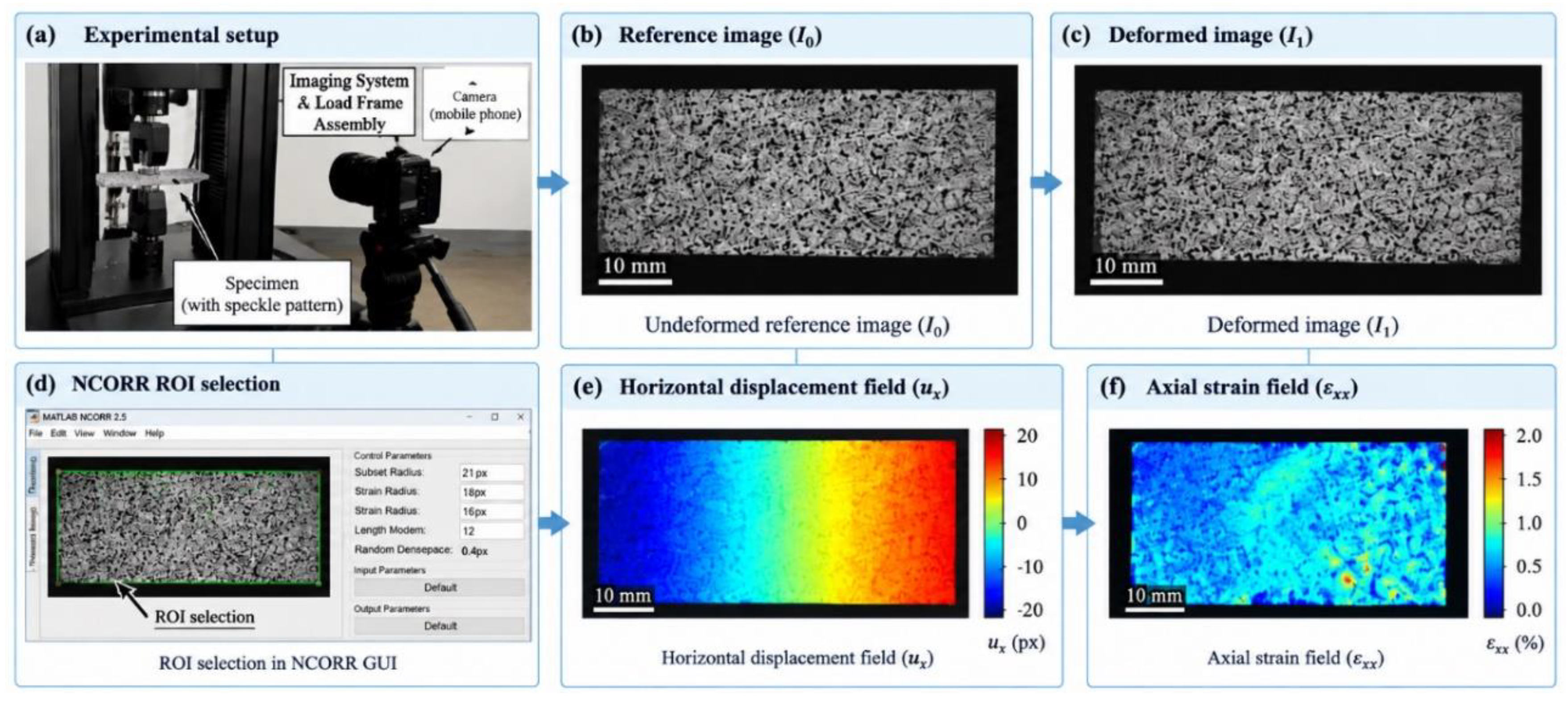
Figure 2.
OpenCV measurement pipeline applied to a planar mechanical component. (a) Mobile phone image acquisition; (b) adaptive Gaussian thresholding result; (c) morphological closing; (d) contour detection and MARR fitting; (e) dimensional extraction and calibration; (f) annotated output image with measurements.
Figure 2.
OpenCV measurement pipeline applied to a planar mechanical component. (a) Mobile phone image acquisition; (b) adaptive Gaussian thresholding result; (c) morphological closing; (d) contour detection and MARR fitting; (e) dimensional extraction and calibration; (f) annotated output image with measurements.
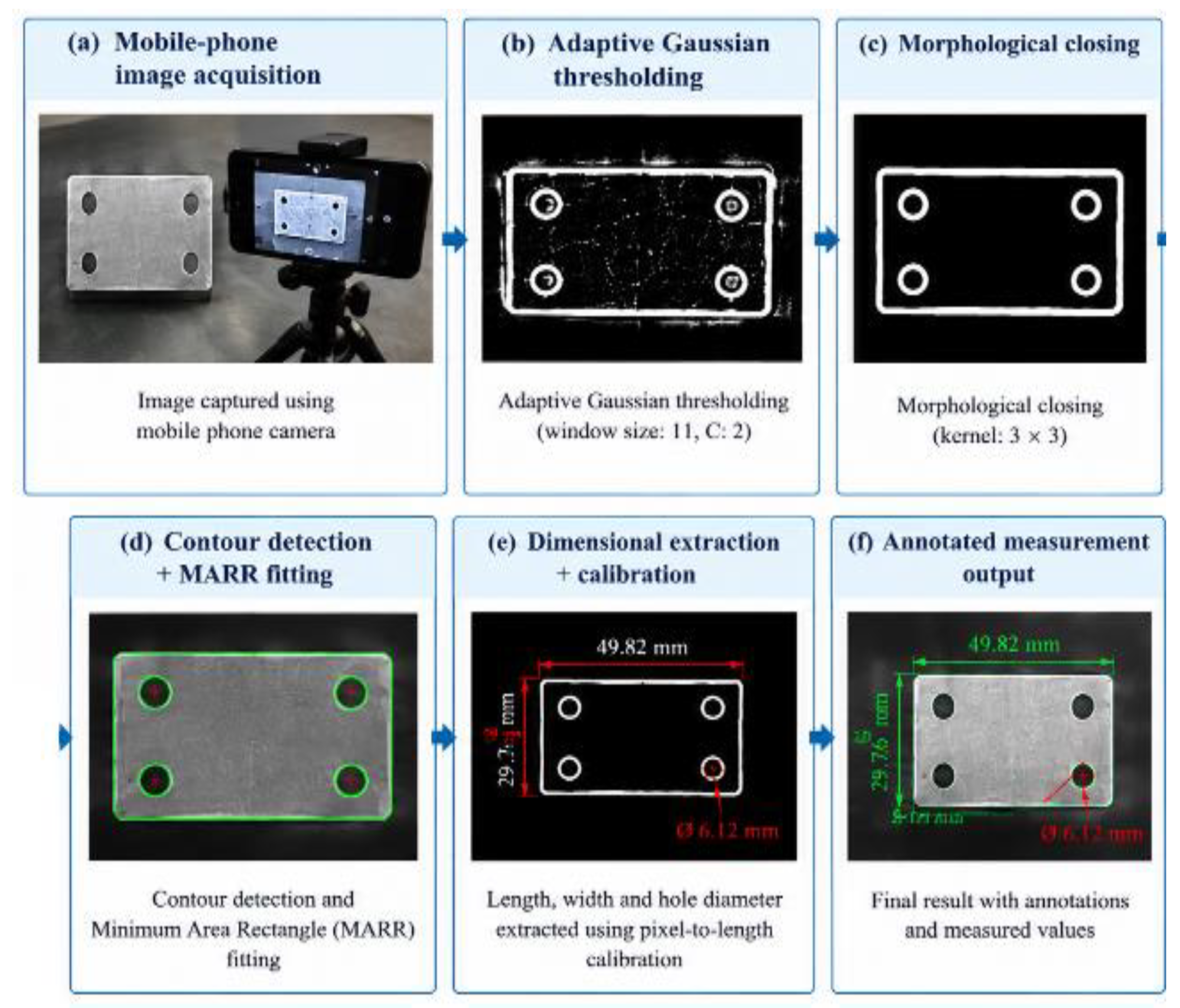
Figure 3.
Phase I annotated output — flat rectangular component. OpenCV MARR-fitted bounding rectangle overlaid on image with dimension annotations: length 161.40 mm, width 76.20 mm, area 12,301 mm². Reference: Vernier caliper 162.00 mm × 77.00 mm.
Figure 3.
Phase I annotated output — flat rectangular component. OpenCV MARR-fitted bounding rectangle overlaid on image with dimension annotations: length 161.40 mm, width 76.20 mm, area 12,301 mm². Reference: Vernier caliper 162.00 mm × 77.00 mm.
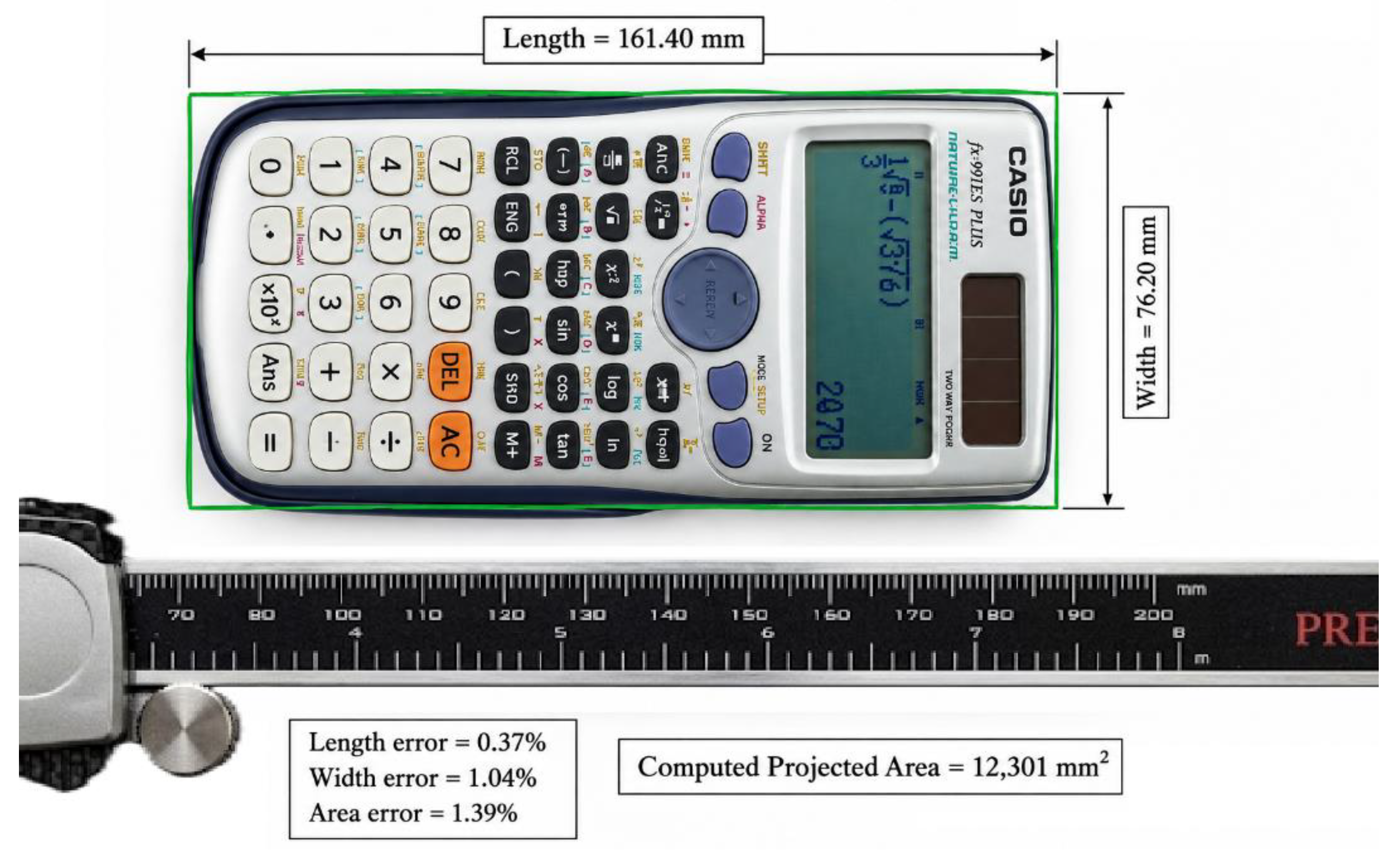
Figure 4.
Phase II annotated output — stepped metallic machine screw. Green line: detected contour; red box: AABR for thread zone; rotated MARR box for total length and diameter. Annotations: Total Length 33.85 mm, Outer Diameter 10.70 mm, Thread Length 16.95 mm. Thread pitch annotation (0.16 mm) is subject to the resolution limitation discussed in Section 4.4.
Figure 4.
Phase II annotated output — stepped metallic machine screw. Green line: detected contour; red box: AABR for thread zone; rotated MARR box for total length and diameter. Annotations: Total Length 33.85 mm, Outer Diameter 10.70 mm, Thread Length 16.95 mm. Thread pitch annotation (0.16 mm) is subject to the resolution limitation discussed in Section 4.4.
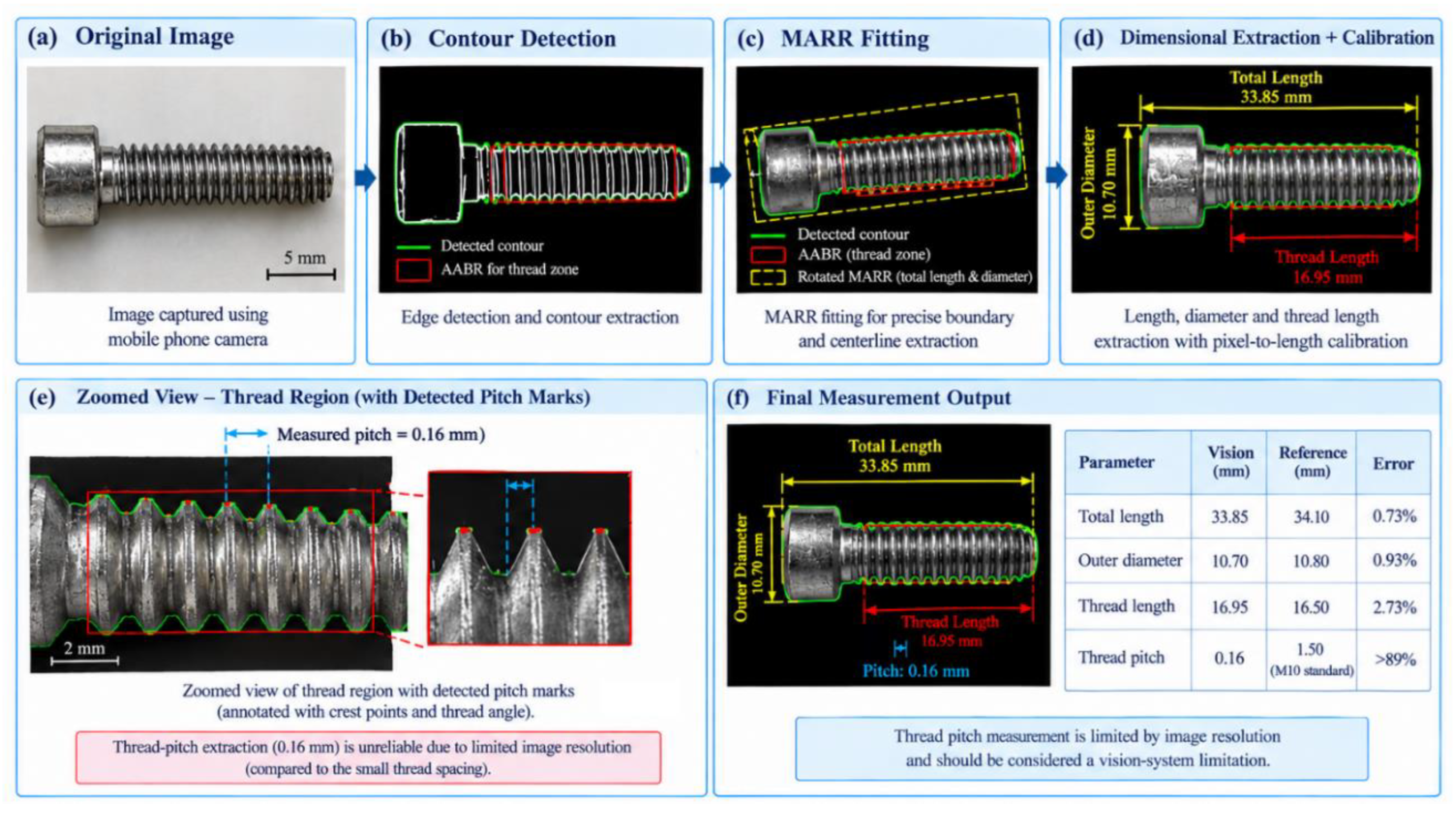

Table 1.
Expected dimensional accuracy as a function of optical configuration. Mobile phone row is derived from the experimental results in Section 4; other rows from reviewed literature [1,2,9,11,13,14].
| Optical Configuration | Pixel Pitch (mm/px) | Sub-pixel Precision (px) | Practical Accuracy | Primary Application |
| Standard macro lens, 4 MP, 80 × 80 mm FOV | ~0.032 | 0.05–0.10 | 0.5–1.0 mm | Structural members, large flat parts |
| Telecentric 1×, 12 MP, 80 × 80 mm FOV | ~0.020 | 0.05–0.10 | 0.1–0.5 mm | Precision flat parts, gear profiles |
| Mobile phone (12 MP, f/1.8), 25–30 cm WD | ~0.050 | 0.10–0.20 | 0.1–0.8 mm (<2% of dim.) |
Workshop inspection, flat parts, fasteners |
| Telecentric 2×, 12 MP, 40 × 40 mm FOV | ~0.010 | 0.05–0.10 | 0.05–0.2 mm | Fine features, small components |
| Microscopic objective 5×, 5 MP, 5 × 5 mm FOV | ~0.001 | 0.05–0.10 | 0.001–0.01 mm | MEMS-scale features, micro-structures [14] |
| Scale | Method | Application Procedure | Notes |
| > 50 mm | Aerosol spray | White primer + matte black spray at 30–50 cm | Accessible; adequate for tensile and bending tests |
| 10–50 mm | Airbrush | White primer + black airbrush; 2–3 passes | Finer speckle; practice required |
| 2–10 mm | Ink stamp / adhesive film | Randomized rubber stamp or inkjet-printed film | Low mass addition; check adhesive stiffness |
| < 2 mm | Lithographic | Photoresist or e-beam deposition [17] | Requires clean-room; reusable for repeated tests |
| Criterion | NCORR | Vic-2D | GOM Aramis | iCorrVision-2D [17] |
| Software cost | Free | Commercial ($) | Commercial ($$$) | Free |
| Platform | MATLAB (license) | Windows/Mac | Windows | Python (free) |
| GUI | Yes — full GUI + API | Yes (full) | Yes (full) | Yes (limited) |
| Displacement accuracy | 0.01–0.05 pixel | 0.01–0.02 pixel | 0.01–0.02 pixel | 0.02–0.08 pixel |
| Strain accuracy | 50–200 µε | 30–100 µε | 30–100 µε | 100–300 µε |
Table 4.
Phase I experimental results — flat rectangular component (scientific calculator). Mobile phone camera at 30 cm; PIXEL_TO_MM = 0.05 mm/pixel; scale-factor calibration.
Table 4.
Phase I experimental results — flat rectangular component (scientific calculator). Mobile phone camera at 30 cm; PIXEL_TO_MM = 0.05 mm/pixel; scale-factor calibration.
| Parameter | Manual Vernier (mm) | Vision System (mm) | Abs. Error (mm) | % Error |
| Length | 162.00 | 161.40 | 0.60 | 0.37 |
| Width | 77.00 | 76.20 | 0.80 | 1.04 |
| Projected Area (mm²) | 12,474 | 12,301 | 173 | 1.39 |
Table 5.
Phase II experimental results— stepped metallic machine screw (threaded cylindrical fastener). Mobile phone camera at 25–30 cm; PIXEL_TO_MM = 0.05 mm/pixel. *Thread pitch error is discussed in Section 4.4.
Table 5.
Phase II experimental results— stepped metallic machine screw (threaded cylindrical fastener). Mobile phone camera at 25–30 cm; PIXEL_TO_MM = 0.05 mm/pixel. *Thread pitch error is discussed in Section 4.4.
| Parameter | Vision System (mm) | Reference (mm) | Abs. Error (mm) | % Error |
| Total Length | 33.85 | 34.10 (Vernier) | 0.25 | 0.73 |
| Outer Diameter | 10.70 | 10.80 (Vernier) | 0.10 | 0.93 |
| Thread Length | 16.95 | 16.50 (estimated) | 0.45 | 2.73 |
| Thread Pitch * | 0.16 | 1.50 (M10 standard) | — | >89% — see 4.4 |
| Projected Area (mm²) | 232.89 | — | — | — |
Table 6.
Measurement method comparison for general planar mechanical components. DOF = degrees of freedom simultaneously captured.
Table 6.
Measurement method comparison for general planar mechanical components. DOF = degrees of freedom simultaneously captured.
| Method | Accuracy | Simultaneous DOFs | Contact? | Dynamic? | Approximate Cost |
| Vernier caliper | ±0.02 mm | 1 (sequential) | Yes | No | ₹500–₹2,000 |
| Outside micrometre | ±0.001 mm | 1 (sequential) | Yes | No | ₹1,000–₹5,000 |
| Dial gauge / LVDT | ±0.01 mm | 1 | Yes | Limited | ₹2,000–₹15,000 |
| Optical profile projector | ~0.01 mm | 2D on screen | No | No | ₹50,000–₹1,50,000 |
| CMM (touch probe) | ~0.5 µm | 3D (sequential) | Yes | No | ₹5,00,000+ |
| Commercial machine vision (HALCON, VisionPro) | 0.1–1 mm | All in-plane | No | Yes | ₹2,00,000+ license |
| Commercial DIC (Vic-2D, GOM Aramis) | 30–100 µε | Full-field | No | Yes | ₹5,00,000+ license + HW |
| Python OpenCV (mobile phone) | <2% of dim.; 0.1–0.8 mm | All in-plane (discrete) | No | Yes | ₹0 software; mobile phone only |
| MATLAB NCORR (open-source) | 50–200 µε | Full-field | No | Quasi-static | ₹0 software; MATLAB license required |
Table 7.
Measurement method comparison for general planar mechanical components. DOF = degrees of freedom simultaneously captured.
Table 7.
Measurement method comparison for general planar mechanical components. DOF = degrees of freedom simultaneously captured.
| SR | Gap | Consequence | Direction |
| 1 | Thread pitch accuracy limited by image magnification at mobile phone scale | Horizontal projection gives >89% error for M10; not suitable for engineering use | Hough Line Transform on thread flank angles; higher magnification lens |
| 2 | No validated integrated OpenCV + NCORR workflow on a single specimen | Full characterization requires two separate setups currently | Single-session workflow using shared image sequence (proposed in Section 5.2) |
| 3 | NCORR MATLAB dependency | Free DIC inaccessible without MATLAB license | Systematic benchmarking of iCorrVision-2D [18] against NCORR on standard specimens |
| 4 | Dynamic DIC for vibrating components not demonstrated with open-source tools | High-frequency loading requires strobe illumination; no NCORR protocol available | High-speed camera + strobe LED; incremental correlation algorithms |
| 5 | Out-of-plane error not quantified for thin components | Planar homography assumes zero out-of-plane motion; thin sheet metal may violate this | Tilted-plane calibration; stereo camera correction for thin specimens |
Disclaimer/Publisher’s Note: The statements, opinions and data contained in all publications are solely those of the individual author(s) and contributor(s) and not of MDPI and/or the editor(s). MDPI and/or the editor(s) disclaim responsibility for any injury to people or property resulting from any ideas, methods, instructions or products referred to in the content. |
© 2026 by the authors. Licensee MDPI, Basel, Switzerland. This article is an open access article distributed under the terms and conditions of the Creative Commons Attribution (CC BY) license (http://creativecommons.org/licenses/by/4.0/).
Copyright: This open access article is published under a Creative Commons CC BY 4.0 license, which permit the free download, distribution, and reuse, provided that the author and preprint are cited in any reuse.