

Submitted:
21 May 2026
Posted:
21 May 2026
You are already at the latest version
Abstract
Critical binding of quantum states in Screened Coulomb Potentials such as Yukawa/Debye, Hulthén, and ECSC (Exponential Cosine Screened Coulomb) potentials is of perennial interest and relevance in many fields of science, ranging from nuclear and particle physics; plasma physics, astrophysics, cosmology, and nuclear fusion; physical chemistry, condensed matter, and materials physics; to synthetic nanostructures and nanophotonics. The purpose of this paper is to heuristically explore two related mysteries, one new, the other more than 50 years old. The solutions to these mysteries have implications for a much broader class of potentials, those addressed by Klaus and Simon. In our recent paper [1], we presented numerical calculations using the Phase Method (PM), accurate to 60 digits and to screening lengths D ≤ 103 au, l = 0–20, of the critical binding parameters for these potentials; an for Yukawa and ECSC, l = 0–12, to D ≤ 105 au, at 30 digits. In doing so, we discovered anomalous period-40 sawtooth structure in the critical parameters of the ECSC potential that is not observed for the Yukawa potential. In this second paper, we quantitatively explain the origin and periodicity of this newly discovered structure. To do so, we use two complementary approaches: a “neoclassical” (NC) variant of conventional semiclassical phase space quantization; and the PM for very precise fullyquantum calculations. The observed period-40 sawtooth structure is quantitatively explained in terms of a novel “tick-tock” mechanism. The periodicity is calculated in terms of the ratio of phase-space integrals for the primary and secondary potential wells. A quartic double-well potential is used as a simple model to further illustrate the tick-tock mechanism. Using NC, an approximate expression is derived to predict the locations of tick-tock glitches from higher order wells; it is confirmed by a PM calculation up to D ≤ 106 au. The second mystery is a strangely linear dependence of the total number of bound states vs screening length for both the Yukawa and ECSC potentials. Using the PM we confirm and extend these empirical relations. We show using the PM that an approximate trivariate linear relation between the square root of the critical screening length √Dc, state number n, and angular momentum l applies to these potentials. This, plus a geometrical state accumulation argument solve the second mystery. We show these properties derive from the scaling relation between screening length and coupling constant, and as such are predicted to be applicable to the whole class of potentials. These results are expected to be of both theoretical interest and experimental relevance when interpreting spectra or calculating thermal properties. The significance of these results, and the applicability of these methods and conclusions to a vast array of related potentials is briefly discussed. Tables of critical screening parameters for Yukawa, Hulthén and ECSC D ≤ 105 and l = 0 − 12 are posted as supplementary data.
Keywords:
screened Coulomb
; critical screening
; critical binding
; ECSC potential
; plasma physics
; Schrödinger equation
; phase method
; semiclassical
; neoclassical
1. Introduction
1.1. Background
Critical binding in Screened Coulomb potentials such as Yukawa/Debye, Hulthén, and ECSC potentials has remained a phenomenon of intense and sustained interest for nearly a century. The fundamental question concerns the precise values of the screening (Debye) length at which quantum states of various angular momenta just become bound or unbound, which has both theoretical and practical ramifications. This question has stimulated a very large body of scientific work by a wide spectrum of physicists and mathematicians, for both bound states and resonances at positive energy. In our current paper we confine our attention to critical binding parameters – the same methods are suitable for calculating eigenvalues however.
Our recent paper [1] was the stimulus for exploring the first mystery addressed in this paper, and the landmark work by Rogers et al [2] and Lam and Varshni [3] are the stimulus for exploring the second mystery. Some familiarity with our first paper is strongly recommended for contextualizing the contents and methods used in this second paper.
Recent progress has been reviewed in [4,5,6,7], with applications to mapping the parameter space of the generalized exponential cosine screened coulomb potential, and attention to circular Rydberg states. A good collection of earlier citations on ECSC potential can be found in Dutt [8].
Recently (2026) we have made a first contribution [1] to this literature which can be viewed as a prelude to the current paper – the two papers naturally go together. From our very accurate computed critical binding parameters we discovered anomalous structure in the ECSC critical screening values, with a strikingly regular periodicity in the vs n plots. This is most clearly visible when the generic trend is divided out, as shown in Figure 1 and Figure 2. The contrast between the Yukawa and ECSC curves is dramatic. Hulthén values are smooth, like those of the Yukawa.
The ECSC potential, (where – for simplicity we omit writing the centrifugal potential), is identical to the Yukawa/Debye potential , except (crucially) for the modulating factor. This factor gives the potential an infinite sequence of positive energy barriers, and associated negative energy wells, the magnitudes of which are damped by the exponential decay and factors. Evidently both Yukawa and ECSC potentials reduce to the Coulomb potential as , i.e. .
A primary goal of our current paper is to explain the origin of this sawtooth structure and its surprisingly regular periodicity . Another goal is to solve a second mystery that apparently has remained unsolved for more than 50 years: the strangely consistent linear relation between the total number of bound states vs for both the Yukawa [2] and ECSC [3] potentials. We will quantitatively solve both of these mysteries, using the complementary methods employed in our previous paper: the Phase Method (PM), and our variant-semiclassical (“neoclassical", NC) method, which extends the accuracy and range of application of standard quasi/semi-classical method for calculating eigenvalues, here adapted instead for the purpose of calculating critical parameters. The rationale for NC is briefly explained below, and in [9]; several useful formulae using it also are given below.
The PM method revealed the sawtooth structure, and NC and PM methods allow us to explain it and its consistent period of , and also to predict the -values at which the higher order wells produce similar behavior. A simple equation is given to predict these, and such a prediction is confirmed using the PM for all screening lengths up to au. We further use the PM to explore this “tick-tock” mechanism with modified ECSC potentials. A simple quartic model system is considered from the point of view of both methods to further illustrate the “tick-tock” mechanism responsible for the sawtooth structure. The NC method is further used to explain the approximately linear vs n and l in light of the scaling symmetry between and coupling constant, which is characteristic of this class of potentials. Finally, the combination of this linear relation with a simple geometrical state counting procedure derived from it, solves the second mystery. Connection with the Coulomb SO(4) symmetry in the asymptotic limit also is discussed.
We predict these latter results are relevant to the whole class of short-range, linear coupling constant potentials that were studied in the seminal paper of Klaus and Simon [10].
1.2. Overview of New Results in This Paper
Our current paper contains a substantial number of new results. To assist the reader we list most of them below, preceded by the subsection number where they are introduced, and tagged by the method(s) used. Results that are carried over from our previous paper for continuity are shown in parentheses.
- PM: Tables of , accurate to 30 significant digits, for Yukawa, ECSC, and Hulthén potentials for all states au and evailable as supplementary data
- 1.3 (PM: sawtooth structure exists in ECSC, constant period 40 for )
- 2.1 (review of Phase Method PM)
- 2.2 explanation of Neoclassical approach NC
- 2.3 NC: example: homogeneous potentials, with formulae
- 2.4 NC: example calculation of Yukawa number of bound states vs to relative accuracy for all l, n, two parameters each, with code
- 3.1 PM: modified potential: sawtooth structure depends on secondary well
- 3.1 PM: modified potential: period of sawtooth structure depends
- 3.1 PM: modified potential: onset of sawtooth structure depends on height of barrier
- 3.2 NC: period 40 quantitatively explained by “tick-tock” mechanism:
- 3.2 NC: sawtooth structure reproduced ab initio using neoclassical approach
- 3.3 NC: approximate formula for locations of tick-tock glitches from higher wells
- 3.4 PM: confirmation of prediction of first tick-tock glitch from tertiary well
- 3.5 NC+PM: example tick-tock calculation for asymmetric quartic double-well
- 3.6 (PM: plot Yukawa vs plot, compare to Rogers 1970)
- 3.6 PM: plot ECSC vs , compare to Lam and Varshni 1972
- 3.6 PM: plot Hulthén vs , same linear trend as in seen for Yukawa and ECSC
- 3.6 PM: vs plot shows ECSC states are clustered by principal quantum number
- 3.7 PM: ECSC vs mystery is solved by arithmetic series accumulation of states
- 3.7 PM: plots of vs n and l show near-uniform density of states for all potentials
- 3.7 PM: geometrical state accumulation solves the second mystery for all three potentials, but begs the question re the reason for the near-linearity, addressed next
- 3.7 (PM: Yukawa contour plots showed striking near-linear relation between , n, l)
- 3.7 PM: contour plots for Hulthén and ECSC also show same
- 3.7 PM: linear fit coefficients determined between , n, l; residual contour plots
- 3.8 First order perturbation theory gives near-linear contour plot for Yukawa
- 3.9 NC: partial derivatives with respect to parameters under phase space integral gives numerical estimates of coefficients, that compare well to fits to PM data
- 3.9 NC: explanation for trivariate linear relation given in terms of scaling symmetry
- 3.10 NC: linear relation further explained in terms of and scaling symmetry, ODE condition for strict linearity
- 3.10 NC: explicit approximate expressions for for Hulthén, Yukawa, ECSC
- NC these properties derive from linear coupling constant a la Klaus and Simon
1.3. Anomalous Sawtooth Structure in vs n
In our previous paper [1] we presented calculations to 60-digit-accuracy of critical screening parameters (inverse screening (Debye) lengths up to au for Yukawa/Debye, Hulthén, Pseudo-Hulthén, and Exponential Cosine Screened Coulomb (ECSC) potentials, for angular momenta – 20. Initial results also were briefly presented up to for – 12 at 30 digits precision for Yukawa, and ECSC potentials. These tables, plus additional tables for the Hulthén potential, are key data used in the current paper, and are deposited as supplementary data for others to use.
The asymptotic dependence of the critical screening lengths for the various bound states (indexed by the integer n for each l-manifold), to which all l curves converge for large , is . Dividing out this asymptotic trend reveals more interesting structure, as shown in Figures 1 and 2, for Yukawa and ECSC respectively. The sawtooth structure in ECSC is striking, and demands explanation.
There are several reasons this structure may have gone unreported previously. One is that it is a subtle deviation from the smoothness of the raw data, and most clearly seen when the predominant dependence is divided out. Another is the upper range of has to be high enough for the periodicity of the jumps to be seen clearly. These data extended to . A third possibility is that hints of such structure indeed might have been seen, but went unreported because there was no explanation for it, and an isolated glitch may have been thought to be a numerical error. Using the highly accurate and robust PM and extending the range made the sawtooth structure very clear. Its nature and origin are explained below, as well as other properties of all ECSC, Yukawa, and Hulthén potentials.
1.4. Nature of Yukawa, ECSC, and Hulthén Potentials
In the critical binding problem, we are concerned about state-binding at zero energy. In the following we will explicitly write the centrifugal potential term. The behavior is rather different depending whether or , so we will normally treat these cases separately. In r-space, as is described at length in our first paper [1], screened Coulomb potentials can show structure on very long length scales, depending on the value of , and with very shallow potential-well depths, but such that bound states can form under the right conditions. gives the Coulomb limit.
For many purposes it is useful to change variables to . In that case, the Yukawa [13] (effective) potential becomes . Evidently, for any finite value of l, as in the asymptotic large n limit, the finite value of l becomes irrelevant, and the behavior is independent of l. As shown in [1] the classical turning points (at zero energy) are , and , where . W is the Lambert W function (ProductLog in Mathematica). The 0 or in the first argument of W specifies the appropriate branch of the function. These are the roots of the equation . If , is a monotonically increasing function, approaching zero as , with a Coulomb-like attractive singularity as . In this case and and . If , there is a positive repulsive singularity as , which, combined with the long range attractive potential from the exponential term, under the right combination of and l, can create a well at that is sufficient to bind a state. This is analyzed in detail below.
The Hulthén [14] potential is of similar form as the Yukawa Potential, but it replaces the factor of the exponential with a factor, where . This behaves much the same as the Yukawa potential at small r but approaches the constant for large r. We can use a similar analysis [1] to the others in z-space, in which . This function has a single peak similar to the Yukawa case, with a peak at and a value at the peak , where, again W is the Lambert W function. Classical turning points must be found numerically by root-finding, but this is straightforward. The value of and give a concise summary of the tradeoffs between l and regarding the ability to bind states.
The ECSC [3] (effective) potential in z-space takes the form . As in the Yukawa potential, for there is an attractive singularity that is dominated as by a repulsive singularity for . The ECSC potential differs from the Yukawa potential by the modulating factor which introduces an infinite sequence of positive energy barriers alternating with negative energy wells, both of which are affected by the value of and l, that have anti-correlated effects. increasing induces more state-binding, while increasing l does the opposite. The value of to some extent expresses the trade-off between them. This is put to further use in subsection 3.7.
For , the turning points are simply , for the primary well; , for the secondary well; and , for the tertiary well etc. These are discrete wells because of the positive energy barriers between them. For , numerical root-finding of is used to determine the turning points, depending on the value of as given above. The function has single discrete smooth peaks within each well; root-finding is straightforward, provided does not exceed the maximum value of at its peak , which provides an upper limit on l (for fixed ) and a lower limit on (for fixed l) at which a state might possibly become bound. Each well in the ECSC potential effectively has its own corresponding and , corresponding to their own ranges of z. The multi-well structures are analyzed in detail below in regard to phase space quantization of the wells.
2. Materials and Methods
All computations were done using code written by the author in Mathematica V14.3 [11].
In this paper, as in our previous one, we primarily use two methods in tandem: “Phase Method” as described in our first paper, a precise and robust fully quantum computational approach; and a variation on conventional semiclassical method that we call “neoclassical” (NC).
A note on terminology: the NC approach is principally based on classic foundational work of Dunham [15], and further elaborated by Bender [16,17]. It is adjacent to a vast body of semiclassical theory from which it differs significantly but only in a specific and narrow way, and it is not in conflict with it. In an attempt to prevent confusion, we refer to it as “neoclassical” (NC). This terminology is by analogy with classical music – neoclassical music (e.g. Stravinsky, Prokofiev) honored and respected the classical forms and ideas, but also reinterpreted them, and applied them to new ends. We do a similar thing here.
2.1. Phase Method
The Phase Method [1,9] is a robust, simple to use, and accurate method for calculating eigenvalues (and as needed, wave functions) by direct solution of the time independent Schrödinger equation for 1D, central, or other separable potentials, which can be smooth, discontinuous, or random; and it handles near-degeneracies very well. It is related t o conventional Shooting Methods, but differs from them in several ways, e.g. by seeking divergent solutions, instead of convergent ones – in what we call the “Shoot First” method. The PM is a significant extension beyond that. It automatically finds all of (a finite number of) states within a specified range energy range using a parallel evolutionary search process; importantly, it does not require any guessing of eigenvalues, assumptions about parity, or tweaking of initial conditions to obtain convergence. Accuracy of eigenvalues to 30–60 digits or more is routine. Fewer digits is fine too – the ultimate accuracy is “dialed-in” by the choice of number of digits of working precision in the calculation. The PM runs very well on ordinary desktop computers, even those with a minimal memory footprint, typically in minutes for most potentials and a few dozen eigenvalues. The run time scales more or less with the number of eigenvalues. It uses arbitrary precision arithmetic, so it is not currently suited for running on GPUs, but otherwise is highly parallel. It should run well on everything between Raspberry Pi computers (with its bundled Mathematica) to supercomputers. These calculations were mostly done on several 16GB M4 Mac Minis.
In our previous paper [1] we applied the PM to the calculation of critical screening parameters for screened Coulomb potentials, to 60 digit accuracy. Adaptation to the critical screening problem required only minor changes to our simple eigenvalue code that is posted for download on our website. More information on the workings of the PM and consideration regarding its application near zero energy is described in [1].
2.2. “Neoclassical” Variant of Semiclassical Method
In our recent paper [1] and book [9] we introduced a continuous real parameter, , in conjunction with phase space quantization, which needs further discussion. Its use represents a narrowly focussed but significant deviation from the standard semiclassical development, while remaining fully compatible with it. In fact its justification goes back to very early exact WKB theory. In using this modified approach here we restrict our attention to determination of energy eigenvalues, or equivalently, critical binding parameters. We do not need to compute asymptotic forms of wave functions by semiclassical means, which entails more detailed exposition [17,18,19,20,21]. Our neoclassical approach, in contrast, is very simple and direct, but still sufficient for our purposes.
As highlighted by Bender [16], the 1932 paper by Dunham [15] contains a foundational equation. It is equivalent to Bender’s [16] equation 10. Dunham extended the earliest WKB formulations by deriving an exact expansion in powers of ℏ, and expressed the energy quantization condition in terms of an infinite sum of contour integrals in the complex plane, where the integration contours enclose the classical turning points. This is elaborated in Bender and Oszag [17]. The various terms in the series involve successively higher derivatives of .
Crucially, single-valuedness of the wave function requires the infinite set of contour integrals to sum to an integer times . This is the fundamental quantization condition for energy levels that we use. Instead of evaluating them term by term, however, we divide the total sum into two parts: the zeroth order term (classical Bohr-Sommerfeld-Wilson phase space integral), plus the total sum of all the rest, which we call . The value of the first order term depends on the behavior at the turning points, and typically simplifies to a constant (e.g. ); we incorporate that value into our parameter . Each of the odd order terms higher than the first evaluate to zero, but the even order terms generally do not. This behavior is explained in Bender and Orszag [17]. The higher order terms typically introduce correction terms that can be expressed as a function of energy, or in other ways. We approximate as a constant plus a decreasing function of n, such as a Padé Approximant, an inverse power series in n, or a decreasing power law or exponential. For many purposes just setting to a constant is sufficient, but the value generally will differ from the canonical one, which is based on the truncated series. In principle this can be made exact using a suitable function of n.
Each successive term in the exact WKB expansion contains increasingly higher order derivatives of the potential; it can be viewed as a kind of gradient expansion. Many others e.g. [16,17,20,21,23,24,25,26] have explained this approach very well. But all of them truncate the series at low order, in part because of the difficulty in evaluating the various contour integrals of higher order. Bender and Orszag go the farthest in evaluating these terms, and examining convergence of the series. Liverts and Barnea [22] evaluate higher order terms, to good effect. Smooth potentials can be rather accurately represented by the lowest order terms; some, e.g. harmonic oscillator and Morse potential, naturally terminate after a couple of terms.
This approach was developed in [9] for computing eigenvalues in homogeneous potentials, and others. Useful equations are given below using for homogeneous potentials. We use this NC method below for approximating critical binding parameters for the doubly-infinite set of n and l values for the Yukawa potential, which are calculated to relative precision, using a simple function, a decreasing power law needing only two parameters each in n, and in l. The calculation is implemented in about a dozen lines of code (shown below); it executes in less than a millisecond on a laptop computer.
The lowest order term in this expansion gives the most rudimentary Bohr-Sommerfeld-Wilson quantization, in which the phase space integral – i.e. twice the integral between the classical turning points of the momentum, expressed as a function of position – is equated to an integer multiple n of Planck’s constant . This BSW criterion is equivalent to requiring that the approximate wave function vanish at the classical turning points – i.e. an integer number of half-wavelengths resides between the classical turning points. This is what one gets when solving the classical Hamilton-Jacobi equation. But this usually gives a rather poor estimate of the true eigenvalue (except for the infinite square well, for which the criterion is exact), because tunneling actually occurs in most cases, which lowers the energy. Instead, rather than viewing the BSW value as a poor approximation to the true eigenvalue, we have argued [9] that it is more useful to view it as an inclusive upper bound on the true eigenvalue; and the BSW value is an exclusive lower bound. The value of interpolates between those limits in n-space. is, in part, a measure of the degree of tunneling.
Bender and Orszag [17] show that the usual value of (for systems with two smooth turning points) emerges naturally from direct evaluation of the first order term of Dunham’s series. Alternatively, arguments from topology and symplectic geometry [18,19,20] give the the same result; the topological concept “Maslov Index” is often applied in this context. This increment to n is an integer multiple of , but it is only part of . Yet, the still-neglected higher order terms can be quite limiting to the accuracy at low quantum numbers, and for rapidly varying potentials. These limitations of the standard formulation have caused many to view the use of phase space quantization for determination of eigenvalues for small n to be unacceptably inaccurate. In the NC approach, the implicit summation of all the terms in Dunham’s series is in principle exact, and applicable down to , to hard potentials, or both.
The conventional low-order truncation of the series, although convenient, introduces other difficulties, which require workarounds. For central potentials with centrifugal potential terms, the “Langer Replacement” modifies the exact factor in the centrifugal potential to , which effectively adds a positive term to it, giving accurate results despite use of the truncated WKB expansion. In this case the two approximations (truncation, and Langer l-shift) are arranged to cancel each other.
For the typical two-sided well, would imply there is no tunneling. If it implies moderate tunneling; this is the standard WKB value, and it is exact for harmonic oscillators, and Morse Potentials. Potentials that are softer (e.g. , ) than harmonic oscillator have slightly larger values than , but not much, and are still considerably less than 1.
Our development of both the NC and PM started with thinking about “mechanical similarity” [27]: the requirement of consistent dynamics in Lagrangian mechanics for similar-shaped trajectories, upon rescaling them in space and time. This analysis is quite different from ordinary dimensional analysis. The effects on the Lagrangian of rescaling of space and time implies that for homogeneous potentials of degree k, energy must scale with action S as where . Our thought, then, was that in the most basic form of semiclassical quantum mechanics, BSW quantization of the action integral also quantizes the energy, and there must be a simple scaling formula for the energies in homogeneous potentials. This indeed is the case, and results are presented below, to illustrate the NC approach. After becoming aware of the existence of the exact Dunham formula, as elaborated by Bender et al [16], we realized such an approximate expression could be made exact by incorporating the “Dunham-shift” (). Furthermore, the phase-space-quantization with Dunham-shift approach evidently also applies to arbitrary (not only homogeneous) potentials. Of course this begs the question as to what is the correct value of , but there is no disputing that indeed does have a value. That observation alone is sometimes sufficient; there are many alternative routes to answering the question of what’s .
We adapt this NC approach to calculating critical screening lengths values at zero energy. Instead of finding energy eigenvalues for a fixed potential/screening length, instead we find the critical screening length at a fixed energy, i.e. zero. The Phase Method implementation is essentially the same. In our previous paper we further used the NC approach to determine the asymptotic dependence of n on , and conditions for circular Rydberg states to form.
2.3. NC Applied to Homogeneous Potentials
As mentioned above, this approach allowed us [9] to derive simple formulae for the approximate eigenvalues of positively homogeneous potentials of the form
where evidently and a are energy and length scale parameters, and k (real-valued, not necessarily integer, or even rational) is the degree of homogeneity of the potential, and is a dimensionless parameter; m is the (reduced) mass. Expressions similar to equations 2 and 3 (apart from the crucial introduction of the parameter ) have been independently derived by others, but their expressions are different in form, and the omission of implies that, as written, they fail for infinite square well, whereas our expressions are exact and smoothly interpolate in k.
Rather than being absorbed by the parameter , we have kept the prefactor of to ease comparison with the most basic benchmark, harmonic oscillator. Here we briefly present these expressions because they illustrate the utility of NC method, and also simply are useful, even for those (e.g. students) with just scientific calculators/apps at their disposal.
First, for such potentials, it is not difficult to show [9] that the eigenvalues scale exactly with the dimensional parameters as . This allows known eigenvalues for any k computed for a given set of potential parameters and a, or values of ℏ, or mass m, to be rescaled for any other potential parameters (of the same k).
Second, we derived a simple generic formula, applicable for :
We have since learned that a similar formula was independently derived by Quigg and Rosner [21] and perhaps others. Again, the key ingredient is the variable , which allows these formulae to perform well at low n and for hard potentials, where usually WKB dare not tread.
This simple expression allows for easy determination of the dependence on n of eigenvalues in different homogeneous potentials. For example for a Coulomb potential, for which , and . As , . Harmonic oscillators have with . As the behavior enters an interesting realm of singular potentials and exponential scaling of bottomless eigenvalues, a discussion of which is outside the scope of the current paper.
The key question here is the precise value (or function) to choose for . Fortunately the ansatz is useful without needing to know precisely. The choice of its value is guided to a first approximation by the ordinary (topological, negative) Maslov-index, but deviations from it are not only allowed but indeed required in most cases, because they account for the missing terms in the exact Dunham expansion.
In this paper we will express , where is the canonical value (e.g. ) and is a decreasing function of n (or l). But even a constant approximate can improve accuracy for low n but still become irrelevant as , except for potentials with infinitely hard walls such as infinite square well. In such a case is appropriate because there is zero tunneling. For a general potential, the correct values of can be determined accurately by back-solving for the required to give the exact (or precise) values such as those from the Phase Method. This was mapped out for homogeneous potentials in [9], in which case was well-represented by a Padé Approximant for all n and k.
As an example of this approach, our approximate eigenvalue equation [9] has the form
where , and we number quantum states . As before and . This equation is exact for harmonic oscillators, and for the infinite square well, and it interpolates smoothly between and , and down to . As above, the prefactor of is retained to facilitate comparison with harmonic oscillator. Other authors have derived equivalent formulae (albeit written differently), but with the key difference being our introduction of the variable , which allows the formula to provide improved range and applicability, even for infinitely hard potentials and low n. One-sided potentials can be handled by considering only the even-n (odd parity) states (we number states .
2.4. calculating Yukawa Values Using Neoclassical Phase Space Method
A larger point we wish to make is that introducing these neoclassical corrections gives us permission to apply phase space quantization methods down to very low quantum numbers, and also to rapidly varying potentials. We will make extensive use of this in our analytical work later in this paper.
By way of illustration here we give a specific example of the Yukawa/Debye potential; the same method applies to other potentials. Here we set the energy for the task of calculating critical screening lengths, in which we seek the values of that just barely increment the number of bound states. We apply the Floor function to to do this quantization, but it is instructive to consider the continuously variable first.
Numerically calculating the phase space integral is straightforward, particularly in . Later in this paper we give usefully-accurate closed-form approximate expressions for the values of these integrals. Here we do it by numerical integration. First, specify the potential for the given parameters and l; find the classical turning points , for those parameter values; numerically integrate between them; and double the result. This gives ; then , where is our continuously variable NC parameter, a deviation from the conventional semiclassical WKB/Maslov index.
As a concrete example, below is executable NC code to calculate ( relative error) estimates of the number of bound states for the Yukawa Potential for specified l and , where (lesser values of can have no bound states and J will be complex-valued). This incorporates, in a primitive way, small dependencies of with n or l at low quantum numbers – estimates of would be rather poor using nominal semiclassical values. The second argument n has an effect only for . The and cases are different in character because of the attractive singular potential for . The parameters an, bn, al, bl are rough and certainly could be improved, as could the primitive functional form for itself; this code is just a simple example. The results can be compared with the extremely accurate PM tables given in [1]. For , since depends on n, the correct value of needed to obtain a particular n can be found by self-consistent iteration, or by root-finding, or tabulation + interpolation to obtain an inverse function. For no such iteration is needed, in this approximation. Similar code can be written for other potentials, for which the turning points can be determined by root-finding instead of analytically, as they are here. Another useful approximation can be found section 3.10.
nbound[l_,n_,D_]:=(
U=-(D Exp[-z]/z)+(l(l+1))/(2 z^2);
beta=(l(l+1))/(2 D);
W=ProductLog; z1=-W[0,-beta]; z2=-W[-1,-beta];
J=Quiet[2 NIntegrate[Sqrt[-2 U],{z,z1,z2}]];
If[l==0,nu0=0,nu0=1/2];
an=-0.034603; bn=-0.44314; al=-0.079887; bl=-0.83606;
deltanu[l1_,n1_]:=If[l1==0,an n1^bn,al l1^bl];
nb=J/(2 Pi)+nu0+deltanu[l,n];
Return[nb])
3. Results
3.1. Numerical Experiments Using PM Calculations on Modified ECSC Potentials
The contrast between the Yukawa and ECSC plots in Figures 1 and 2 is dramatic, and the multi-well structure that is present in the ECSC potential is an obvious hypothetical candidate to explain it. We first wish to determine if this is true, then determine a mechanism.
The Phase Method that was used to calculate critical binding parameters to 60 digit accuracy in our previous paper is sufficiently simple and robust that it easily can be (and was) used to perform numerical experiments on modified ECSC potentials. One question is whether the secondary ECSC potential well between is essential for the observed sawtooth structure shown in Figure 2.
To test this, we did a simple numerical experiment in which the secondary well is filled-in (i.e. set to zero). This experiment used the same code and ranges that were used for calculating the accurate tables in our previous paper, but with the modified potential. We see in Figure 3 that filling-in of the secondary well totally eliminates the sawtooth structure over the range au. Both and calculations are shown.
In another set of numerical experiments using the PM, the depth of the secondary well was multiplied by a “well scale factor” of wsf=1, , and 2. The resulting sawtooth structure is shown in Figure 4. It is seen that the period scales approximately as , which is explained below in terms of ratios of phase space integrals of primary and second wells.
In the third set of numerical experiments using the PM, the barrier between the primary and second wells was scaled by a “barrier scale factor” of bsf=, , 1, 2, and 4. The results are shown in Figure 5. It is seen that the height of the barrier has little effect on the period, but reducing its height advances the position of first onset, and increasing it delays the onset.
From these numerical experiments it is clear that the second well is key to explaining the observed sawtooth structure over the indicated range. It will be shown below that tertiary and higher wells also contribute at much larger values of .
3.2. Neoclassical (NC) Explanation for Sawtooth Structure Observed for ECSC Potential
The previous subsection clearly shows the role of the second well in generating the sawtooth structure. We will analyze this structure from the point of view of a “neoclassical” (modified semiclassical, with variable ) approach described in subsection 2.2, in which the usually-neglected higher order terms in the exact infinite WKB series are approximated by an additive term: a constant, or a smoothly decreasing function of n or l. Here, for simplicity we will focus on the states, but the same kind of analysis applies to the higher l states, but with slightly greater complexity. Examples of this will be shown in subsection 3.10 in connection with explaining the linearity dependence of the total number of bound states on screening (Debye) length . As usual we will use atomic-like units in which ℏ and the reduced mass of the two-body system are both equal to 1.
For our purposes here, the phase space integral is the integral of momentum over position for a full cycle of classical motion in a bound state: , where and are the classical turning points at energy , i.e. those points at which , and is the effective potential including the centrifugal potential if .
We are interested in critical binding of states at , and in this subsection we confine our attention to , which makes the turning points independent of and l. Changing variables to , we have for the first well of the ECSC potential: where ; for the second well where . Crucially, for , both phase space integrals scale exactly as , so that dependence divides out. For the scaling is not exact, because an l-dependent term in the integrand prevents dividing out , and because the classical turning points (limits of integration) also depend on and l Yet the relation still holds approximately. In subsection 3.10 the interplay between the dependencies on and l for is analyzed in detail.
The quantization condition for binding of a state within each (separate) well is of the form and similarly for well 2. The floor function gives the largest integer that is . Later we will it useful to consider the continuous-valued variable , before the floor function is applied to it. The parameters and differ slightly from the well-known canonical values derived from topological considerations (yet still are based on the approximate, truncated WKB expansion), which are 0 and respectively for well 1 (with singularity) and well 2 (no singularity or hard walls). Here we choose values of and . The choices of these values are representative, and were selected to give rough agreement with a few low-n and low l values, PM values, is not critical to our overall conclusions.
The combined state count for the two wells taken separately is then . It might be argued that it it is the combined phase space area that should be quantized: but we find the results are more consistent with separate quantization of the wells. We note the inequality , so the scenario with two separately quantized wells has equal or fewer bound states. The combined state count is then . As increases, the main well accumulates bound states, and at a critical level, the second well start to bind a state. The relative rates at which they bind states is given by the ratio of . Crucially the common factor of divides out. In the sawtooth diagram the abscissa is the total state count +. It’s analogous to two clocks, one ticking 39 times until the second clock tocks once, and the process repeats. The total number of states accumulated in a ticktock cycle is close to 40, which is that which is observed in the sawtooth diagram for . The values of and affect the initial onset, but not the period. We call this the "tick-tock" mechanism.
Using this model a calculation of the curve corresponding to the curve in Figure 2 was generated, and it is shown in Figure 6. To do so, the function was evaluated on a grid of au up to . The transition points were detected in one line of code (First@GroupBy in Mathematica); the plot is given below. We see that it compares very well with corresponding curve in Figure 2 which is based on 30-digit accuracy PM calculations. In particular, we see several attributes are well-reproduced: the sawtooth structure; its nominal period of 40; the locations of the minima ; and the values of the curve themselves. The precise locations of the minima are affected somewhat by the approximate “neoclassical” parameters; the tick-tock period of “40” is simply a pure number with no adjustable parameters: .
Calculating the curves for in the same manner is only slightly more complex, because of the dependence of the turning points on l and , but the essentials are the same. This sort of calculation is done below for comparison of Hulthén, Yukawa, and ECSC potentials for arbitrary l, for the purpose of explaining the strangely linear dependence of the total number of bound states vs .
At this point we consider the first mystery to be solved, but there is more to investigate about it.
3.3. Subsidiary Wells of Higher Order
This tick-tock mechanism also extends to the infinite number of progressively shallower wells at larger z that are characteristic of the ECSC potential, and should give rise it an infinite number of “tockitos” for sufficiently large . The question is where they occur. It is not difficult to estimate (and indeed numerically evaluate) these phase space action integrals in z-space, with . We number the higher wells as . The well is localized between . Replacing the integrand over that interval by its value at its average z value , and multiplying by its width , with a correction factor c on the order of one to account for its shape (which is quite similar for all m), we get with .
Then in our usual way we find where , or a simple neoclassical adjusted value . Solving for the screening length required to bind states, we have . Evaluating the required to bind one state and using we get for respectively au, au, au, au, or approximately 21 nm, 22 m, 18 mm, and 13 meter. Furthermore the period of such sawtooth oscillations for the well would be about 1293, compared to 40 for the well. As a consequence it might be expected for such a single tick-tock glitch to be observed experimentally (e.g. in spectra) for the well, in addition to the expected sawtooth/tick-tock structure from the well. The range of needed to observe the second and higher sawtooth glitches is quite extensive, however, as it varies as the square of the state number. In the next subsection we address this using the PM.
3.4. Sawtooth Structure from Higher Index Wells
The spatial locations of the wells for in -space occur at , , , …, or more concisely with . The primary well corresponds to , the secondary well , etc. For and the wells are uniformly spaced in z and their shapes are very similar to each other, but with very large (-fold) reduction in depth between successive wells. This regularity makes estimating the well depths and phase space integrals straightforward by scaling successive wells, and using a common shape factor c on the order of 1 to approximate the integral. In this way we obtain a simple approximate expression for the phase space integral for any , which agrees sufficiently well with numerical integrals. We use a NC parameter with a value near (specifically ) for the wells ; and for , a value near zero (specifically ), owing to the potential singularity. These deviations from the canonical semiclassical values are small but important corrections that are essential to obtain usefully accurate results for low n. They could be improved but these are sufficient for our purposes here.
Setting we obtain an estimate for for any well and any of its bound states : where and . This agrees roughly with more accurate numerical phase space integrals and precise PM values. For simplicity here we neglect small -dependent corrections to , at the expense of some accuracy.
Evaluating this function we see that the first bound state of the tertiary well (, , au), is predicted to be between the ( au) and the ( au) levels of the secondary well, generating a single“tick-tock” glitch there for that series. Specifically, evaluating our simple expression above with predicts the first bound state of the tertiary well should occur at . This would give a downward jump in the curve around that location, but a rather slowly varying one, because of the large -scale.
We subsequently tested this prediction by doing a PM calculation for the ECSC potentials up to a maximum value of . The result is shown in Figure 7. Agreement with the prediction is excellent. If observed experimentally and unexpected, this feature could cause some confusion. The second “tockito” of ( au) state is expected to occur at values that are an order of magnitude greater, i.e. hundreds of micrometers scale. The sequences for the successive wells start to overlap in the region . The corresponding values of in such cases quickly get into the macroscopic length range but those might be relevant for some systems. This is shown in Figure 8.
3.5. Illustrative Tick-Tock Model: Asymmetric Quartic Double Well
It is instructive to consider a simple double well potential as a model of this tick-tock behavior, and to consider it from the points of view of the fully quantum PM method, and the neoclassical NC method.
An example of such a potential is , which is plotted in Figure 10; the right panel also shows a phase space plot evaluated at zero energy. If placed in one of the wells, a classical particle with a total energy less than the top of the barrier, would remain confined to that well. In reality, some degree of quantum tunneling will occur between the wells, and such tunneling will be significantly enhanced for energies near the top of the barrier. If the discrete levels for the two separate wells were to line up with each other, and extensive tunneling were to occur, this could induce substantial splitting between the energy levels, which might have other consequences. However, if the energy levels weren’t extremely close (which in general is unlikely) the two-well system behaves as a combination of two separate wells, but with a combined total state count.
For each well, and at a specified energy, the phase space integrals can be computed as twice the integral of the momentum between the classical turning points. At it corresponds to the areas contained within the left and right regions shown in Figure 9, which correspond to the primary and seconday wells.
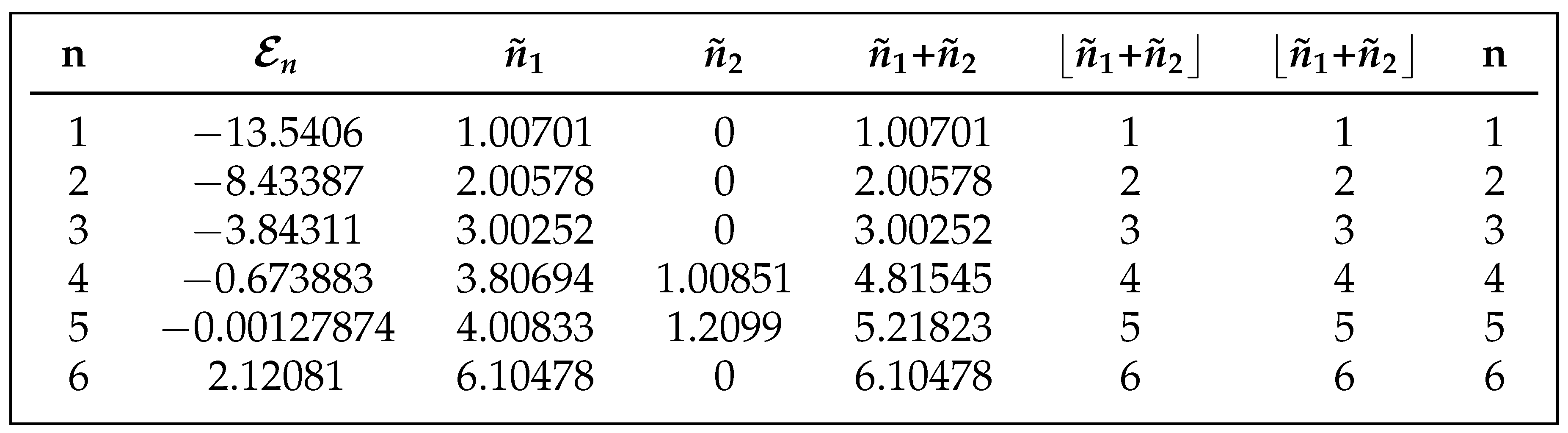
We define a continuous valued . The value of is to a degree affected by the amount of quantum tunneling. When exceeds an integer, a new bound state can form. To compare results between PM and NC, in Table 1 this expression is evaluated for both the left () and right () wells, at the energy if the PM-computed eigenvalue.
Using the Phase Method we computed the energy levels and wave functions for this potential. In Table 1 these energy eigenvalues are given in column 2. We can see in Figure 10 that at lower energies, up to three bound states are confined to the deeper left well, until a new state appears in the shallow right well, giving four states altogether. This is the analog of the first tick-tock state. A second state is spread across both wells at the slightly negative fifth eigenvalue. The sixth and higher states are continuum states are spread across both wells.
The PM wavefunctions, and in particular, their squares, the corresponding probabilities, reinforce this picture. The states reside entirely within the left well, but the probability in the fourth level for the first time is concentrated in the right well. The fifth energy level which is only slightly bound has probability distributed across both wells, as does the sixth, which is at positive energy.
Figure 10.
PM-calculated probability distributions (squared wavefunctions) for the asymmetric quartic double-well potential. The probability (squared wavefunction) is shown, superimposed on the potential to show where it is spatially distributed.
Figure 10.
PM-calculated probability distributions (squared wavefunctions) for the asymmetric quartic double-well potential. The probability (squared wavefunction) is shown, superimposed on the potential to show where it is spatially distributed.
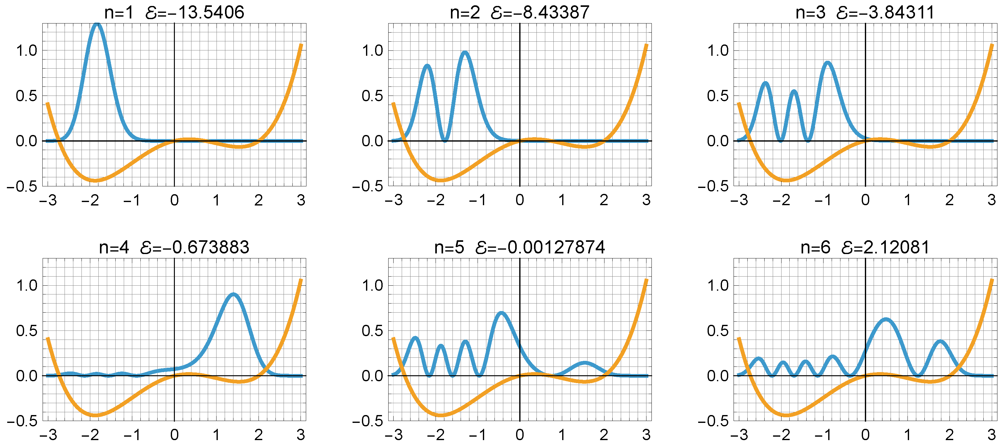

Table 1.
Comparison of fully quantum PM calculations and neoclassical phase space quantization for the two wells. The first and last columns indicate the quantum number; the second the eigenvalue. are for the first and second well respectively. , and , small but significant deviations from canonical values, that are related to the extent of tunneling. represents the floor function, i.e. the largest integer .
Table 1.
Comparison of fully quantum PM calculations and neoclassical phase space quantization for the two wells. The first and last columns indicate the quantum number; the second the eigenvalue. are for the first and second well respectively. , and , small but significant deviations from canonical values, that are related to the extent of tunneling. represents the floor function, i.e. the largest integer .
 |
3.6. Solution to the n* Linearity Mystery for ECSC Potential
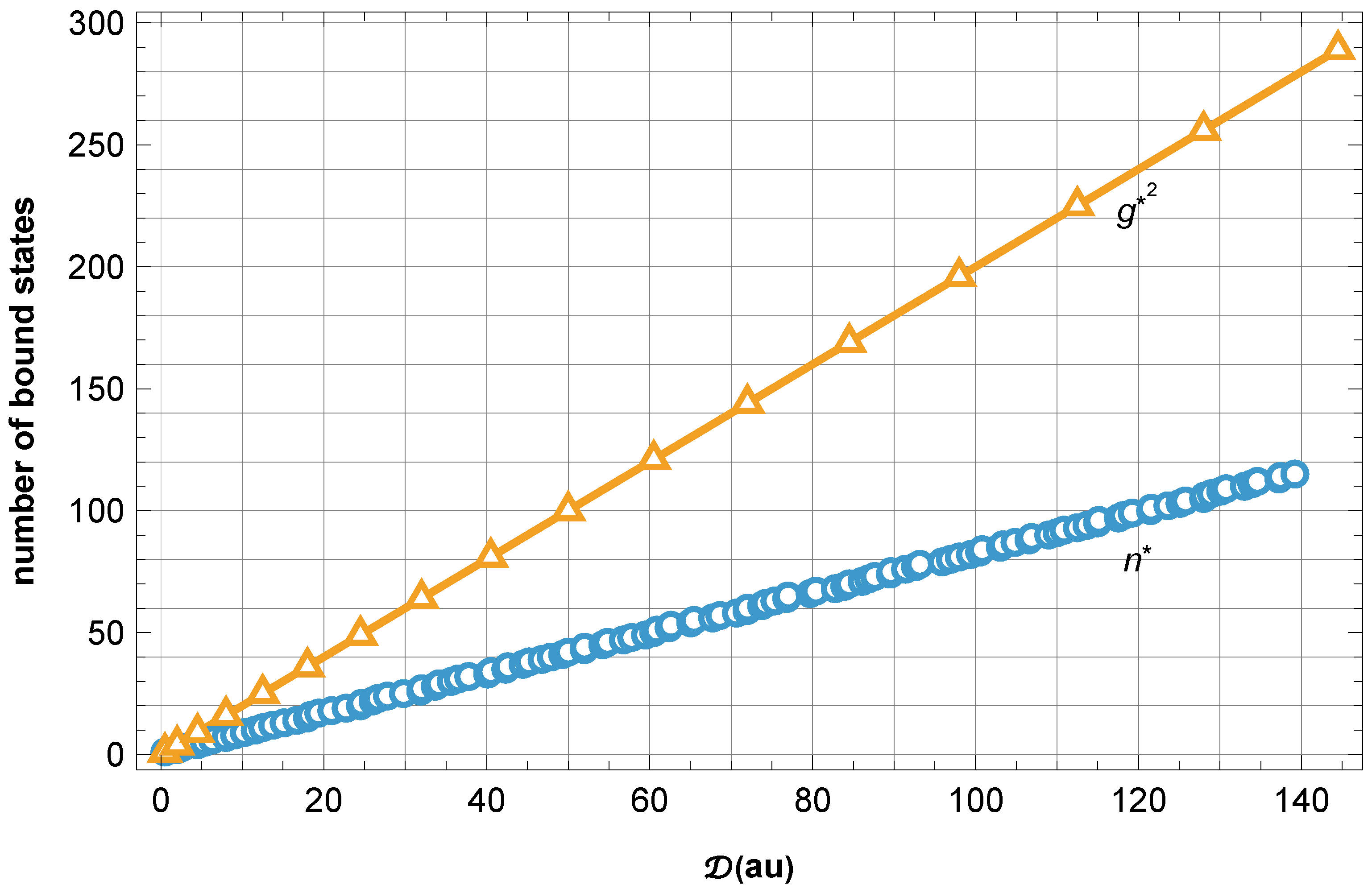
The classic paper by Rogers et al in 1970 calculated critical screening lengths for the lowest 45 bound states of the Yukawa/Debye potential, as well as eigenvalues and other things. They found two approximately linear relationships between the screening length and two quantities: , and , where is quantum number of the highest bound state, and , the total number of bound states of all angular momenta. Our own calculations of critical screening lengths to 60 digits and over a larger range of confirmed and extended the results of Rogers et al. Figure 1 from our first paper [1] is reprised here as Figure 11. The rectangular region marked in the lower left corner indicates the region covered by Rogers et al [2]. Our calculations independently reproduce their results precisely over that region, and also substantially extend the range, over which the linearity persists. Both represent all of the bound states for their specified ranges.
The first of the linear relations, the one involving , is easily explained, as others have done, and we did in our recent Atoms paper, using a simple phase space quantization argument, which indicates the slope of that linear plot is , which agrees well with least squares fits to our PM-calculated critical values. Specifically this says that , and , and .
Similarly, Lam and Varshni’s 1972 paper [3] found linear relationships (of course with different slopes than Yukawa/Debye) for the ECSC potential. The plot refers to states. From phase space argument similar to the Yukawa case we find (using numerical integration) , and , giving a slope of vs of . Both Rogers et al, and Lam and Varshni allowed for nonzero intercept values, and we follow suit for comparison. Fits to our PM-calculated values give with confidence intervals of , respectively. We consider this very good agreement with the semiclassical phase space quantization estimate. Lam and Varshni’s fits give a slope estimate of , but they take pains to point out these values are underestimates of the slope and intercept, owing to the under-sampling of the data points. For this reason we consider their values and ours to be in sufficient agreement, although our contemporary values are much more accurate.
Yet what has been missing for more than a half-century, to our knowledge, is any explanation for the second linear relation involving the total number of bound states . The striking high degree of linearity is mysterious, because the underlying dependence is . In this subsection we present a solution to this mystery.
In Lam and Varshni’s plot for the ECSC potential, in contrast with Rogers et al’s plot (and our Figure 12) for the Yukawa potential, the points do not lie as consistently on the best fit line for the plot. Their state counts are slightly under-sampled, as pointed out by the authors. Here we plot our ECSC potential results in the same manner which as shown in Figure 1. These curves represent all the bound states with no undersampling issues. Lam and Varshni’s -range stops right before the sawtooth structure emerges in our plots.
In contrast to the Yukawa potential in Figure 11, In Lam and Varshni’s [3] Figure 2, the points on the line are bunched-up into distinct groups, with gaps in-between. Some tendency to downward curvature of each group also is visible. Our Figure 12, based on our PM calculations, with range selected for comparison with [3]. shows all of the bound states up to the maximum value, and it is quite revealing. First we note that only a single state first appears on the line, then a doublet, then a triplet, and so on. Inspecting the nature of the states (we computed them, so we know what they are) we find that they correspond to states of the same principal quantum number, and in the usual atomic ordering: (1s), (2s, 2p), (3s, 3p, 3d), (4s, 4p, 4d, 4f) etc. In the ECSC potential no level-crossings are observed over the entire range that was calculated up to au. The total number of states below a selected s-state (which are easy to locate as above using ) with , is then just the arithmetic sumof the number of states in each complete group below it, which evaluates to a state-count , or for moderate . This is encouraging.
Although the dominant term varies as , the expression also includes a term proportional to , which reduces the slope slightly; yet the curve remains sufficiently close to linear. The quantum graininess adds a measure of apparent noise (which it is not). Fitting the arithmetic sum estimate derived above over the range to a simple proportionality (with zero intercept) gives a function , importantly, with a residual between fit and curve that does not deviate by more than 1 (bound state) unit, and so it is within the quantization graininess of the computed data points. The determined slope also is in reasonably good agreement with the slope of a linear least square fits to our own high precision PM-computed values, and also is consistent with Lam and Varshni’s self-proclaimed lower bound .
We conclude the linear n* plot for the ECSC potential is explained using basic phase space quantization and considerations of the arithmetic sum state accumulation that is appropriate in this case. This was relatively simple because the states of different principal quantum number did not overlap – there were no level crossings, a fact that emerged from the accurate PM calculations. This is not the case for Yukawa and Hulthén potentials, however, so a more general approach is needed, which we investigate next.
Figure 11.
Plot of (square of maximum number of bound states; and (total number of bound states of all l) as a function of screening length , for the Yukawa potential. The inset corresponds to the range covered by Rogers et al [2] Figure 5. g* is the higher bound state; n* is the maximum number of all bound states for any l.
Figure 11.
Plot of (square of maximum number of bound states; and (total number of bound states of all l) as a function of screening length , for the Yukawa potential. The inset corresponds to the range covered by Rogers et al [2] Figure 5. g* is the higher bound state; n* is the maximum number of all bound states for any l.
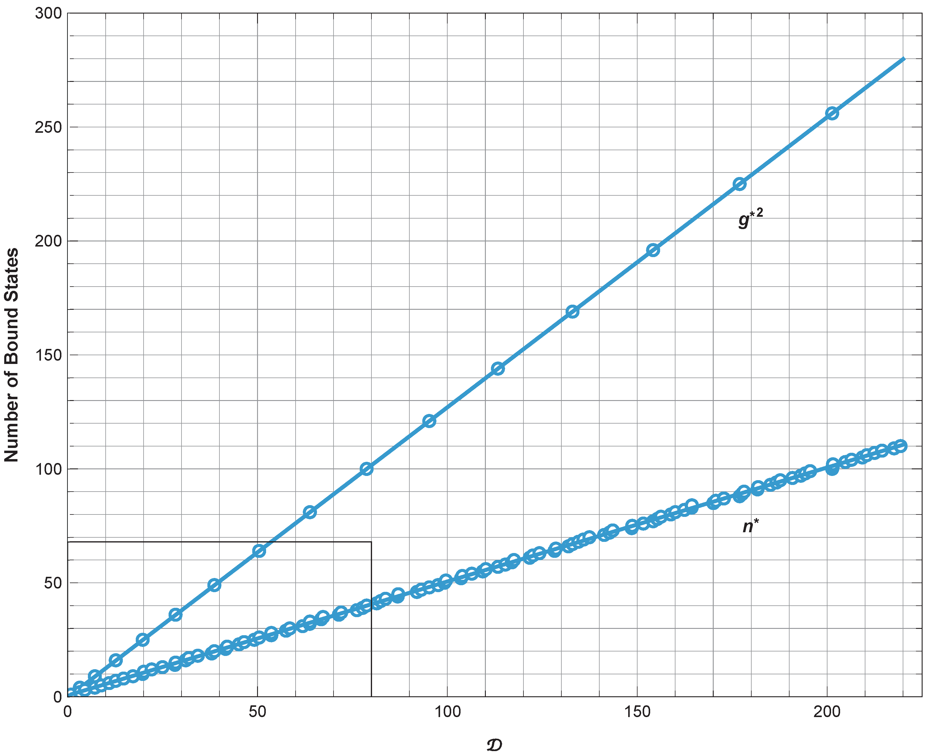
Figure 12.
Plot of g*2 (square of maximum number of bound states; and n* (total number of bound states of all l) as a function of screening length , for the ECSC potential. The range is chosen for comparison with Lam and Varshni [3] Figure 2. The first tick-tock glitch is slightly above this range. Calculations were done by the Phase Method as described previously. Note the 1-2-3-4… state binding pattern observed along the n* line. These correspond to (1s), (2s, 2p), (3s, 3p, 3d) etc. A similar pattern is not found for the other potentials because the states of different principal quantum number overlap for them.
Figure 12.
Plot of g*2 (square of maximum number of bound states; and n* (total number of bound states of all l) as a function of screening length , for the ECSC potential. The range is chosen for comparison with Lam and Varshni [3] Figure 2. The first tick-tock glitch is slightly above this range. Calculations were done by the Phase Method as described previously. Note the 1-2-3-4… state binding pattern observed along the n* line. These correspond to (1s), (2s, 2p), (3s, 3p, 3d) etc. A similar pattern is not found for the other potentials because the states of different principal quantum number overlap for them.
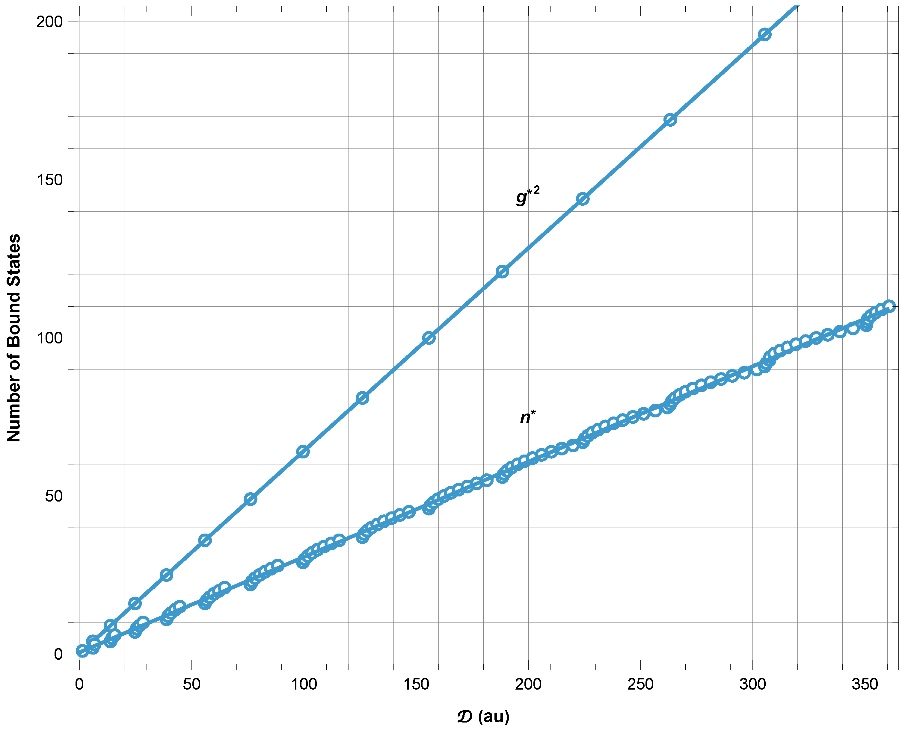
Figure 13.
Plot of g*2 (square of maximum number of bound states; and n* (total number of bound states of all l) as a function of screening length , for the Hulthén potential. The range is limited so that no states for fall within the data range, as they are not represented in the dataset. Calculations were done by the Phase Method as described previously. The same kind of linear behavior is found as for Yukawa and ECSC potentials.
Figure 13.
Plot of g*2 (square of maximum number of bound states; and n* (total number of bound states of all l) as a function of screening length , for the Hulthén potential. The range is limited so that no states for fall within the data range, as they are not represented in the dataset. Calculations were done by the Phase Method as described previously. The same kind of linear behavior is found as for Yukawa and ECSC potentials.
3.7. Geometric Solution to the vs Linear Relation Mystery
The values for Yukawa and Hulthén potentials do not show the convenient grouping by principal quantum number that is seen for the ECSC potential. We can “unfold” the states according to both n and l by plotting the values for each state vs n, or l, with all states being represented. These show a startling regularity, as can be seen in Figure 14 and Figure 15: the density of states in this representation is seen to be nearly uniform. This solves the mystery: the total number of states below a specified threshold value is proportional to the area of the triangular region below it. This area grows in proportion to the square of the threshold, i.e. . This begs the question as to why the potentials have that nearly uniform density, however, a question we address next.
In the previous section we found that, using accurate and complete tables of calculated by the Phase Method, there is a nearly uniform density of states when is plotted vs n, or l. The reason for this mysterious result also requires an explanation, which we pursue in this subsection.
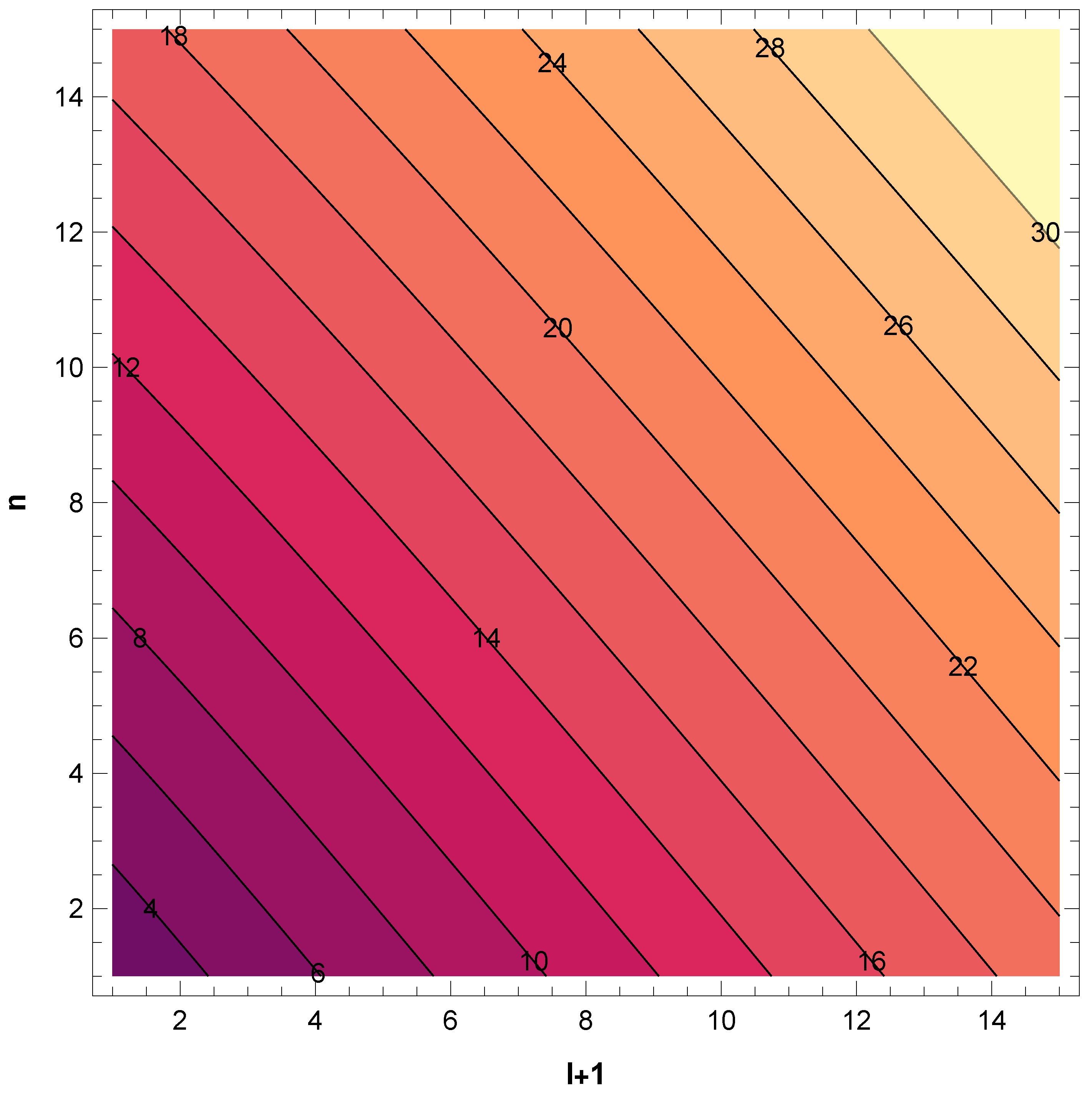
In our previous paper [1], we showed in passing that a contour plot of vs n and for the Yukawa potential exhibited a striking linearity in both variables. Here we extend this analysis to the ECSC and Hulthén potentials, using the tables from [1]. We find very similar results for all three potentials, as shown in Figure 16. The nearly parallel and equally spaced contours for all three potentials indicate a uniform linear gradient of vs n and l (or ), with an additive constant. It is not exact – the residuals are not zero, as shown in the right panels of those figures.
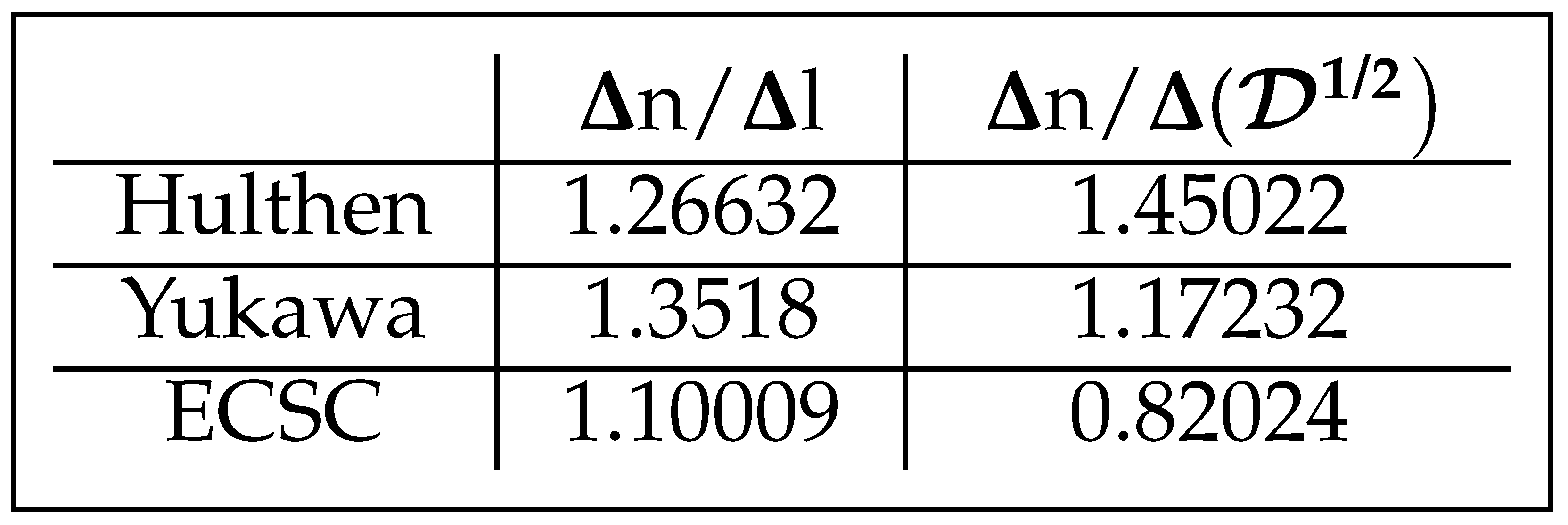
Bivariate linear least squares fits were performed, with best fit parameters and confidence intervals given in Table 2 and Table 3. The ratios of the coefficients are given in Table 4 for comparison with calculations to be given later.
We note that this is contrary to the strict one-to-one relation between n and l found for the Coulomb potential, in which the energy levels depend only on the sum , where is known as the principal quantum number. Incrementing n and decrementing l by one give the same energy. This is a consequence of the famous dynamical SO(4) symmetry of the potential, which does not apply to screened Coulomb potentials. They do, however, show a broken-symmetry version of that 1:1 linear relation.
We predict that other potentials in this class (i.e those that satisfy the scaling law between screening length and coupling constant) will exhibit the same near-linear bivariate relation with n and l. The fundamental reason for this is explained below.
Table 2.
Best least squares fits to PM-calculated linear combination of and n plus a constant.
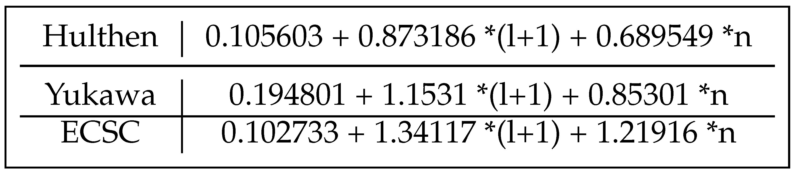 |
Table 3.
Confidence Intervals (95%) for the fit parameters above.
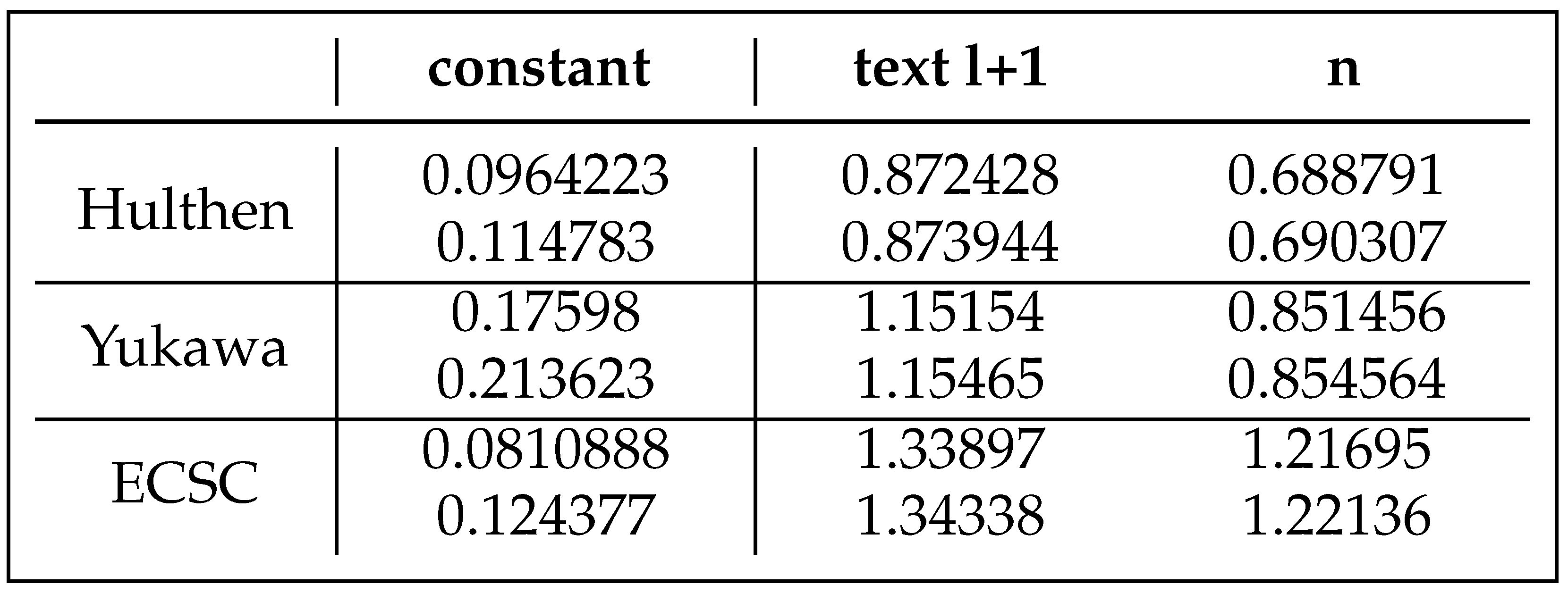 |
Table 4.
Ratios between fit coefficients. See text for explanation.
 |
3.8. Perturbation Theory Calculation of Linear Correlation Contour Plot for the Yukawa Potential
First order perturbation theory also was used to calculate estimates of the values as a function of l and n for the Yukawa potential. Exact Coulomb eigenfunctions and eigenvalues were used for the unperturbed states, and the full difference between the Yukawa potential and Coulomb potential was used as a perturbation Hamiltonian – the centrifugal potential terms cancel exactly. Despite the fact that the unperturbed Coulomb states of a given principal quantum number but different l are degenerate, any nonzero screening parameter lifts that degeneracy, so the use of non-degenerate perturbation theory is still appropriate.
The first order corrections to the eigenvalues are simply given by the expectation value of the perturbation Hamiltonian above within each unperturbed eigenstate. All of the integrals were done symbolically in Mathematica. The perturbation increases the energy of the perturbed eigenstates for each , and the value of required to raise the perturbed eigenvalues to reach zero energy was solved for, and is the estimate of for each state. These are the values shown in the contour plot below.
This first order perturbation theory is approximate, but it is strikingly similar to the others calculated by the far more accurate Phase Method calculations. Our conclusion is this approximately linear relation between , n, and l is intrinsic to the nature of this potential. The PM calculations shown above, and the NC calculations shown below indicate this is a shared feature of this class of potentials, which we will show is related to their scaling symmetry.
Figure 17.
vs and for Yukawa potential, as calculated by first order perturbation theory. The unperturbed potential is Coulomb, and the difference between the Yukawa and Coulomb potentials was used as a perturbation. The displayed values are those values required for the perturbed eigenvalues to be shifted up to zero energy. Computations were done analytically in Mathematica, but are rough in comparison with the PM-calculated values in Figure 9. The key feature of interest is the striking linear relation between and n and l, which is maintained despite the rough approximate nature of this first order PT calculation.
Figure 17.
vs and for Yukawa potential, as calculated by first order perturbation theory. The unperturbed potential is Coulomb, and the difference between the Yukawa and Coulomb potentials was used as a perturbation. The displayed values are those values required for the perturbed eigenvalues to be shifted up to zero energy. Computations were done analytically in Mathematica, but are rough in comparison with the PM-calculated values in Figure 9. The key feature of interest is the striking linear relation between and n and l, which is maintained despite the rough approximate nature of this first order PT calculation.
3.9. Explanation of Approximate Linear Dependence of q, n, l by NC Phase Space Arguments
The striking near-linearity shown in the contour plots above requires explanation, and again phase space arguments provide quantitative insight. The applicability of the neoclassical approach to small n levels extends its reach to problems for which traditional semiclassical analysis might be considered inappropriate.
We found an approximate linear relationship between all three quantities: ; the state number n; and the angular momentum l. In the asymptotic limit we also know the Yukawa Potential becomes the Coulomb potential, which has the known hidden SO(4) symmetry which explains the degeneracy of its energy levels of a given principal quantum number . It is simply the sum of n and l that determines the energy, so there is an inherent symmetry between n and l: increasing one of them by 1 is equivalent to decreasing the other by 1. The near one-to-one alignment of the contours in space in the contour plots presumably reflects the breaking of this symmetry that occurs at finite screening lengths.
We can compute estimates of this correlation for the Yukawa potential using phase space arguments. Analysis of the Hulthén and ECSC potentials is similar. The effective potential in r-space is
As is well-known, and also shown in our previous paper, a characteristic feature of this class of potentials is that scaling the screening length in the exponential by a factor is exactly equivalent to multiplying the exponential term by the same factor. First, we will consider the continuous-valued , taking constant, and restrict our attention to for comparison with the contour plots. Changing variables to , and defining and , our phase space integral becomes
and , are the classical turning points, which are the locations in which the momentum p vanishes.
These evidently depend on a specific combination of and . Defining , as in our previous paper, we have and where W is the Lambert W function (ProductLog in Mathematica). An upper bound on the value of that might bind a state is .
The approximate symmetry between and is evident by inspection, and it follows from the scaling symmetry mentioned above, because that is the origin of the coupling constant coefficient of the exponential term. With the change of variables to z-space, the z-values between and are generally on the order of 1, and so the coefficients of of the and terms are similar in magnitude. The function is the ratio of the two weight coefficients, and it is the roots of that give the turning point solutions. The peak of is at , and its maximum is .
We can make this more quantitative with an explicit computation. Our contour plots in Figure 15 and Figure 16 express q as a function of n and l (or , a difference of little consequence). The neoclassical/semiclassical phase space integral gives us as a function of q and . We can differentiate under the integral with respect to parameters q and (which we will take as continuous). By Leibnitz’s formula, the limits of the integral, which also depend on q and also must be differentiated, but in the case of phase space integrals, those contributions vanish, because the momentum is zero at the turning points: , identifying the momentum at zero energy as times the square root in this integrand. Therefore only differentiation with respect to the integrand itself contributes.
With this useful fact in hand, we find:
Similarly, differentiating with respect to gives
These expressions are respectively proportional to q and , and the integrals are pure numbers that depend on via the classical turning points and . ranges from zero to for the Yukawa Potential. diverges at the turning points but the integrated weight is not very large there. The functions and also have similar z-dependence. The result is that both integrals are very similar in magnitude.
We want to compare with the contour plots that express q as a function of n and l. Here we have as a function of q and . To compare, we have . For fixed we then have and similarly .
Using differentiation under the integral as above, the ratio on the right side of this equation is readily computed numerically for a given q and l, or the composite variable . We have evaluated this numerically over the (integer-valued) feasible pairs q, l i.e. those for which , and examined the results from –30 and –60.
The mean and standard deviation of are and are . These compare well with the coefficients in the linear fit of (dq/dn) and (dq/dl) obtained by linear bivariate fits over the narrower range , that were fit to the PM data in the Yukawa Potential contour plot in subsection 3.7. We find this to be a satisfactory numerical confirmation of the approximate mutual linearity of n, q, l.
The feasible pairs of are those for which , i.e. . This condition can be rewritten , which is a region bounded by the indicated hyperbola in q, l, as shown in Figure 18. The apparently straight line relation between and is actually an asymptote of this hyperbola, with deviations from linearity at low q and l. The constant is small enough the relation is effectively a straight line. The slope of this line asymptotes to , which is in good agreement with the ratios of coefficients of the linear fits in Table 2. These imply that the deviations of the gradient from the (1,1) direction in the contour plots of Figure 16 are characteristic of the form of the potential, and are principally related to the value of for each potential.
We conclude that the linearity of the Rogers et al, and Lam and Varshni plots, as well as our extended range versions of them, and our contour plots, all are explainable in terms of a NC phase space analysis. Differentiating under the phase space integral , predicts near-linear dependence between , l, and n. This is further seen to be a consequence of the approximate symmetry between and in the phase space integral , which is a consequence of the scaling relation between coupling constant and screening length in this entire class of potentials. The relation also reflects the fact that the Yukawa potential breaks the SO(4) symmetry of the Coulomb potential, in which n and l affect spectra in the combination . We expect a similar analysis and conclusion holds for other potentials in this class (e.g. Woods-Saxon), with possible in multiwell potentials such ECSC and generalized ECSC.
3.10. Y-Function Analysis of q, n, l Near-Linear Relation
The q vs correlation is even more intimate than suggested above, which becomes clear when written in terms of the composite variable , and the function (for Yukawa potential – has a different form than this for its sibling potentials); as usual . is determined for a specified screening length and angular momentum l. Only values between are meaningful for the Yukawa potential, and the two roots of the equation determine the classical turning points which are the limits of integration in the phase space integral. In this case they are soluble analytically as and where W is the Lambert W function, ProductLog in Mathematica.
As in [1] we can write the phase space integral where . This tells us that is proportional to but with a residual dependence on q via the composite variable . With , and approximating as a constant, and recognizing that differentiating with respect to the limits gives no contribution as explained above, we have . For strict linearity between and q to occur, this would require . Solving this simple differential equation we get . This is the form of that would give strict proportionality between and q. What we obtain numerically approximates this fairly closely, but not exactly.
Evaluating the integral numerically, tabulating the numerical integral on a fine grid, we find , which very well matches the exact asymptotic (large n) value . Then, fitting the computed (using Mathematica’s NonlinearModelFit) to a power law we obtain an excellent fit: with and , with a coefficient of determination . The power of 0.53446 is close to, but statistically very distinct from, the exact value of that strict proportionality between and q would require. This is consistent with the broken Coulomb SO(4) symmetry that was discussed earlier.
We can also relate these coefficients to other known quantities. The asymptotic value of ; taking this form as correct (hypothetically); and recognizing we must have , we conclude that , where is a precisely defined numerical characteristic of the form of the potential, as in analysis; then the only undetermined parameter is the power , which we have seen is close to but slightly greater than . If were exactly , we would have , a constant, i.e. strict linearity. The actual exponent gives better agreement with the PM data, and introduces slight nonlinearity between q and n.
The same procedure for Hulthén and ECSC potentials (primary well) gives similar results as shown in Table 5 below, which is consistent with the contour plots shown in Figure 16, and the bivariate linear least squares fits to them. This, and the perturbation theory results, support the conclusion the approximate linear relation between , n, and l is a shared intrinsic property of this extensive class of potentials which are expressible in terms of a linear coupling constant, here .
With , the dependence on q and or or l can be determined directly from and the chain rule. Evaluating these derivatives and etc for , gives values within about of those in Tables 2–4.
Table 5.
Fit coefficients of numerically evaluated phase space integrals for the three potentials. Selecting l and specifies , which allows the phase space integral to be approximately evaluated for , i.e. . The slight deviations of values from shows the relation between and is close to, but not exactly, linear.
Table 5.
Fit coefficients of numerically evaluated phase space integrals for the three potentials. Selecting l and specifies , which allows the phase space integral to be approximately evaluated for , i.e. . The slight deviations of values from shows the relation between and is close to, but not exactly, linear.
 |
At this point we consider the nested mysteries contained within our second mystery to be solved. We believe the extended trilinear relation between , n, and l (including a constant offset), which defines a plane in q, n, l space, and the approximation to be potentially useful.
4. Discussion
In our previous paper, discovery of the unexpected sawtooth structure in the vs n plots called out for an explanation. The unusual nature of the ECSC potential – an infinite periodic series of positive energy barriers and negative energy wells – evoked all kinds of subtle and exotic hypotheses (shape resonances, subtle tunneling splittings inducing binding transition, extended states modeled in terms of transmission lines...). However, further analysis, backed up by numerical experiments using the Phase Method (PM) on specifically-modified ECSC potentials, quickly revealed a very different and relatively simple (“tick-tock”) mechanism – as increases, states become bound in the primary well (ticks), but a new channel opens up when sufficient phase space area has accumulated to bind a new state (tock) in the secondary well. This causes an irregularity in the expected smooth accumulation of states (ticks) vs , particularly when plotted vs the total state count (tick+tock). Crucially, the common factor for the two phase space areas divides out exactly, leaving a dimensionless number , where and are the phase space areas of the primary and second wells for . The additive 1 is related to the total state count being the sum of the two contributions. The analysis is more complex and nuanced for , but it is still analytically tractable, in terms of , using methods applied above for the Yukawa potential.
We further extended this analysis to derive a simple approximate equation to predict the approximate locations of all such “tick-tock” glitches. The first such “tockito” for the tertiary well was predicted and subsequently confirmed using a PM calculation up to ; the second todckito is predicted to occur at au. Similar behavior is expected for other multi-well potentials of this type, such as generalized ECSC potentials.
As it is non-standard, the NC method required explanation. It is a simple but nontrivial departure from conventional semiclassical/WKB analysis. It fundamentally is based on the 1932 paper of Dunham, which has been highlighted by Bender [16,17] and reprised in many contemporary quantum mechanics books, but these treatments almost universally truncate to low order Dunham’s exact infinite-order gradient expansion in powers of ℏ, essentially assuming the higher order terms sum to zero or are negligible. In contrast we assume they sum to a finite (usually nonzero) value, the magnitude of which we have shown is related to the amount of tunneling into the potential barrier. This is a simple but useful reinterpretation of a small portion of the vast body of semiclassical theory that has been developed by eminent physicists and mathematicians. Fundamentally, however, we rely on the 1932 paper of Dunham, and the 1977 paper of Bender et al.
The NC approach frees us to tackle states of low quantum number n and/or sharply varying potentials. To illustrate its utility we give examples of its use for homogeneous (e.g. power law) potentials, with a formula for eigenvalues that is exact for both harmonic oscillator and infinite square well, and that smoothly handles potentials of intermediate hardness. The PM and the NC methods proved to be a potent combination. Our previous paper describes the PM; the current paper describes the NC method. Both are explained with many applications in our 2024 book [9].
The NC method next was used to solve the second mystery, which is a peculiar historically noted [2] (but unexplained) linear relation between the total number of bound states and the screening length for the Yukawa potential. Lam and Varshni [3] found a similar relation for the ECSC potential, but a little less well-resolved. In our current paper, from the PM-calculated results first shown here, we demonstrate the linear relation between and also applies to the Hulthén potential. Solving this mystery required solution of several other nested mysteries, one of which involved surprising linear relation that found in our previous paper between , n, and l. This relation revealed, through a geometrical argument, that the total number of states below a threshold grows approximately as the square of that threshold, and hence the number of states grows linearly with . It begged the question underlying the basis of the approximate linear relation between , n, and l.
This we tackled using NC analysis. First we used the scaling relation (applicable to this class of potentials) between screening length and coupling constant (the factor multiplying the attractive exponential term in the potential). By differentiating with respect to and under the phase space integral the near-symmetry of the competing terms in the potential indicate there is a similar but opposing effect of changing q and . Evaluating the integral numerically gives near-linear relations between , n, and l, which solved the second mystery.
The close relationship between n and q for all three potentials is further studied in the last part of the paper, where . Strict linear dependence between n and would require a dependence . All three potentials have a power of close to, but slightly greater than . We predict other potentials in this class of potentials to have similarly close correlations between n, l, and , and to be subject to analysis by these same methods. We expect they will show similar linearity properties.
In this paper we have connected disparate observations that all reduce to a shared common origin, which also indicates its applicability to a far broader group of short range linear-coupling constant potentials, i.e. those addressed by Klaus and Simon [10].
- Based on accurate extensive PM calculations:
- – linear relationship between total number of bound states vs screening length
- – is explained by near-constant density of states in vs n and l observed in plots
- – is explained by near-linear relation between vs n and l, observed in contour plots and fits
- – is explained via NC analysis quantitatively for linear coupling constant potentials
- – near-symmetry between and in scaled (z-space) phase space integral
- – near-linearity related to dependence of phase space integral on .
- – Single-well phase space integral approximately given by: ; where and ;
- – the orientation of the gradient of in q, l space depends on for that potential.
5. Conclusions
Both the accurate full-quantum PM calculations and the NC/phase space integral approach were essential for our solutions to both top-level mysteries addressed in this paper. Tables of for the Hulthén, Yukawa, and ECSC potentials up to au and –12 are deposited as supplementary data.
The primary initial goal of this paper was to understand the origin and nature of the sawtooth structure that was observed in the plots of vs n plots for the ECSC potential, that was discovered in our previous paper [1]. Those high precision values were calculated using our “Phase Method” (PM), which was explained in that paper.
To explain the sawtooth structure paper, we have used those tables, additional numerical experiments using the PM, and a variant-semiclassical method we call "neoclassical" or NC method. This was used to explain the sawtooth structure in terms of a simple“tick-tock” mechanism, which can be expected to also be relevant for other multi-well potentials at large screening lengths. In the NC formulation the observed period-40 emerges naturally in terms of the purely numerical ratio of phase space areas: .
The theoretical justification of the NC method is described, and how and why it differs from conventional semiclassical method. A key benefit of the NC approach is that it can be applied without caveats or reservations to low quantum numbers and hard potentials. In its current primitve form it is limited to calculating energy eigenvalues and critical binding parameters, but this is sufficient for our purposes. Example applications are given to homogeneous potentials. The tick-tock mechanism is illustrated using both NC and PM methods with a highly asymmetric quartic double well potential.
A second goal of this paper has been to understand the strangely linear dependence of the total number of states vs screening length that was observed more than 50 years ago in both Yukawa and ECSC potentials, but unexplained. This is strange because the underlying dependence is , so the rate at which states accumulation with screening length has a very specific character. Solving this mystery turned out to require the solution of other nested mysteries contained within it, all ultimately being reducible to the well-known scaling symmetry between screening length and linear coupling constant to which this class of potentials conforms. Hulthén, Yukawa, and ECSC potentials were all investigated and characterized, but the methods and behavior is expected to apply much more broadly. We also confirmed this linear relationship for the Hulthén potential.
Many of the approaches used in this paper for Hulthén, Yukawa, and ECSC potentials are expected to be equally applicable to other potentials in its class. These specifically are the ones that can be written in terms of a linear coupling constant (here ), as described by Klaus and Simon. Xu et al [5] cataloged nine of them in their appendix, specifically the three addressed here, plus venerable potentials such as Woods-Saxon, Manning-Rosen, Lennard-Jones, Pöschl-Teller, and modifications of them. Based on our NC/phase space analysis, we predict the near-linear relationship between , n, and l, as shown in our contour plots and fits for Hulthén, Yukawa, and ECSC potentials, should also apply to these others (modulo features from tick-tock glitches in multiwell potentials as was found for ECSC).
We hope the tables, methods, insights, and predictions in this paper will prove to be of lasting value.
Funding
This research received no external funding.
Data Availability Statement
Tables generated in this work are freely available for download at https://gbxafs.iit.edu/criticalscreening/ and at the publisher as supplementary data
Acknowledgments
The author wishes to thank his family, friends, and colleagues for their patience and support during this rather-consuming project, and to acknowledge Illinois Tech for office space, library, support facilities, and Mathematica site license. This work includes no content from generative AI.
Conflicts of Interest
The author declares no conflicts of interest.
References
- Bunker, G. B. Numerical Computation of Critical Binding Parameters of Screened Coulomb Potentials I. Atoms 202614, (3) 18. [Google Scholar] [CrossRef]
- Rogers, F. J.; Graboske, H. C., Jr.; Harwood, D.J. Bound Eigenstates of the Static Screened Coulomb. Phys. Rev. A 1970, 6, 1577–1586. [Google Scholar] [CrossRef]
- Lam, C.S.; Varshni, Y.P. Bound Eigenstarte of the Exponential Cosine Screened Coulomb Potential. Phys. Rev. A 1972, 6(4), 1391–1399. [Google Scholar] [CrossRef]
- Xiao, H.J.; Zhang, Y.Z.; Montgomery, H. E., Jr.; Ho, Y.K.; Liu, A.; Jiao, L.G. Complete critical bound region of the generalized exponential cosine screened Coulomb potential. J. Phys. A Math. Theor. 2024, 57(29), 295307–295320. [Google Scholar]
- Xu, L.; Jiao, L.G.; Liu, A.; Wang, Y.C.; Montgomery, H.E., Jr.; Ho, Y.K.; Fritzsche, S. Critical screening parameters of one-electron systems with screened Coulomb potentials: circular Rydberg states J. Phys. B 2023, 56(17), 175002. [Google Scholar] [CrossRef]
- Jiao, L.G.; Xie, H.H.; Liu, A.; Montgomery, H.E., Jr.; Ho, Y. K. Critical screening parameters and critical behaviors of one-electron systems with screened Coulomb potentials J. Phys. B 2021 54, 175002–175015. [Google Scholar] [CrossRef]
- Jiao, L.g.; Xu, L.; Zheng, R.Y.; Liu, A.; Zhang, Y.Z.; Montgomery, H. E., Jr.; Ho, Y.K. Critical screening parameters of one-electron systems with screened Coulomb potentials: high Rydberg limit J. Phys. B 2022, 55(19), 195001. [Google Scholar] [CrossRef]
- Dutt, R.; Chowdhury, K.; Varshni, Y. P An improved calculation for screened Coulomb potentials in Rayleigh-Schrodinger perturbation theory. J. Phys. A Math. General. 1985, 18(9), 1379–1388. [Google Scholar] [CrossRef]
- Bunker, G.B.; Bunker, G. B. The Phase Method: for Numerical Solution of the Schrödinger Equation; Kindle Edition: Oak Park, Illinois, 2024. [Google Scholar]
- Klaus, M.; Simon, B. Coupling constant thresholds in nonrelativistic quantum mechanics. I. Short-range two-body case. Ann. Phys. 1980, 130(2), 251–281. [Google Scholar] [CrossRef]
- Wolfram Research, Inc., Mathematica, Version 14.3. Champaign, IL, 2025. Available online: https://www.wolfram.com/mathematica.
- Singh, D.; Varshni, Y.P. Accurate eigenvalues and oscillator strengths for the exponential-cosine screened Coulomb potential. Phys. Rev. A. 1983, 28(5), 2606–2610. [Google Scholar] [CrossRef]
- Yukawa, H. On the interaction of elementary particles. I. Proc. Phys.-Math. Soc. Jpn. 3rd Series 193517, 48–57.
- Hulthén, L. Über die Eigenfunktionen des Grundzustandes des Deuterons. Ark. För Mat. Astron. Och Fys. 1942 28A, 5, 1–12. [Google Scholar]
- Dunham, J. L. The Wentzel-Brillouin-Kramers method of solving the wave equation. Phys. Rev. 193241, 6, 713–720. [Google Scholar] [CrossRef]
- Bender, C. M.; Olaussen, K.; Wang, P.S. Numerological analysis of the WKB approximation in large order. Phys. Rev. D. 1977, 16(6), 1740–1748. [Google Scholar] [CrossRef]
- Bender, C.M.; Orszag, S.A. Advanced mathematical methods for scientists and engineers: Asymptotic methods and perturbation theory; Springer: New York, 1999; Vol. 1. [Google Scholar]
- Keller, J.B. Corrected Bohr-Sommerfeld Quantum Conditions for Nonseparable Systems. Ann. Phys. 1958 4, 180–188. [Google Scholar] [CrossRef]
- De Gosson, M. Symplectic geometry and quantum mechanics; Birkhäuser: Basel, 2006. [Google Scholar]
- Berry, M.V.; Mount, K.E. Semiclassical approximations in wave mechanics. Rep. Prog. Phys. 1972, 35(1), 315–397. [Google Scholar] [CrossRef]
- Quigg, C.; Rosner, J.L. Quantum mechanics with applications to quarkonium. Phys. Rep. 1979, 56(4), 167–235. [Google Scholar] [CrossRef]
- Liverts, E.Z.; Barnea, N. Transition states and the critical parameters of central potentials. J. Phys. A 2011, 44(37), 375303. [Google Scholar] [CrossRef]
- Landau, L.D.; Lifshitz, E.M. Quantum Mechanics Non-Relativistic Theory; Pergamon Press Inc.: Elmsford, New York, 1977. [Google Scholar]
- Müller-Kirsten, H.J.W. Introduction to quantum mechanics: Schrödinger equation and path integral; World Scientific Publishing Company, 2012. [Google Scholar]
- Griffiths, D.J.; Schroeter, D. F. Introduction to quantum mechanics; Cambridge University Press, 2018. [Google Scholar]
- Zwiebach, B. Mastering quantum mechanics: essentials, theory, and applications; MIT press, 2022. [Google Scholar]
- Landau, L. D.; Lifshitz, E.M. Mechanics; Pergamon Press Inc.: Elmsford, New York, 1969. [Google Scholar]
Figure 1.
Yukawa vs state number . The curves are relatively featureless.
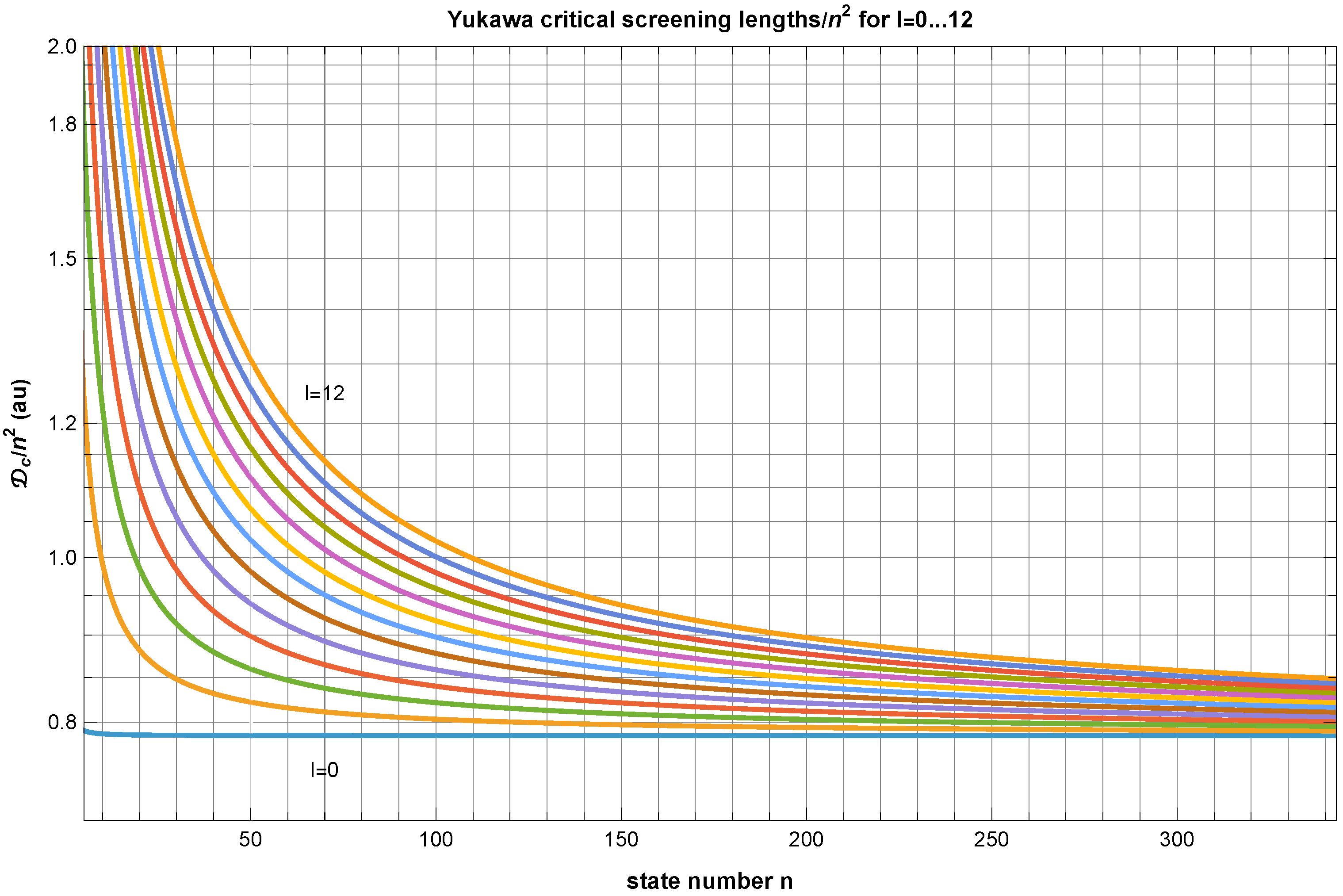
Figure 2.
ECSC vs state number . The structure repeats states.
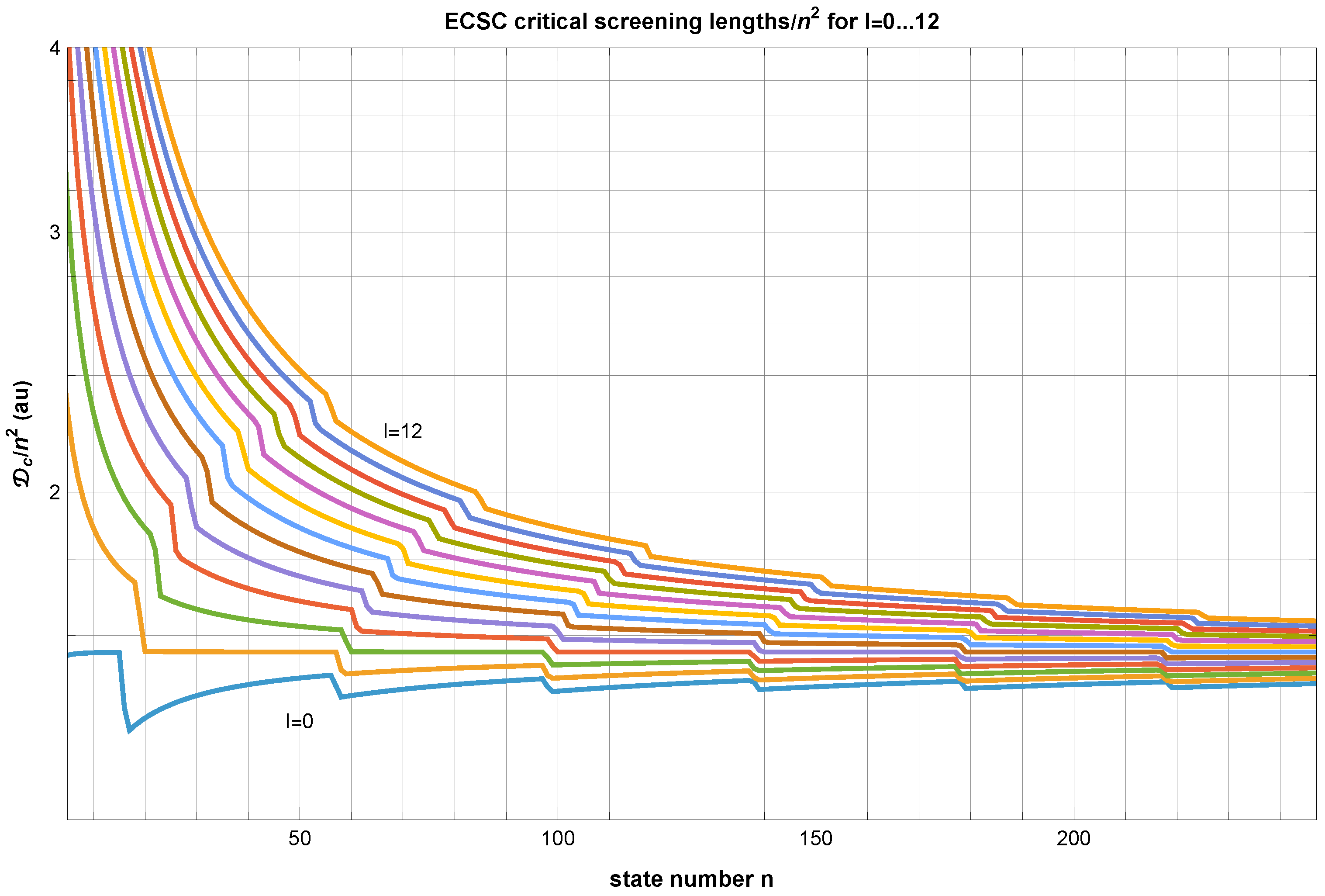
Figure 3.
Comparison of vs n PM-calculated with and without secondary well for and . The secondary well evidently is necessary for the sawtooth structure to appear for au.
Figure 3.
Comparison of vs n PM-calculated with and without secondary well for and . The secondary well evidently is necessary for the sawtooth structure to appear for au.
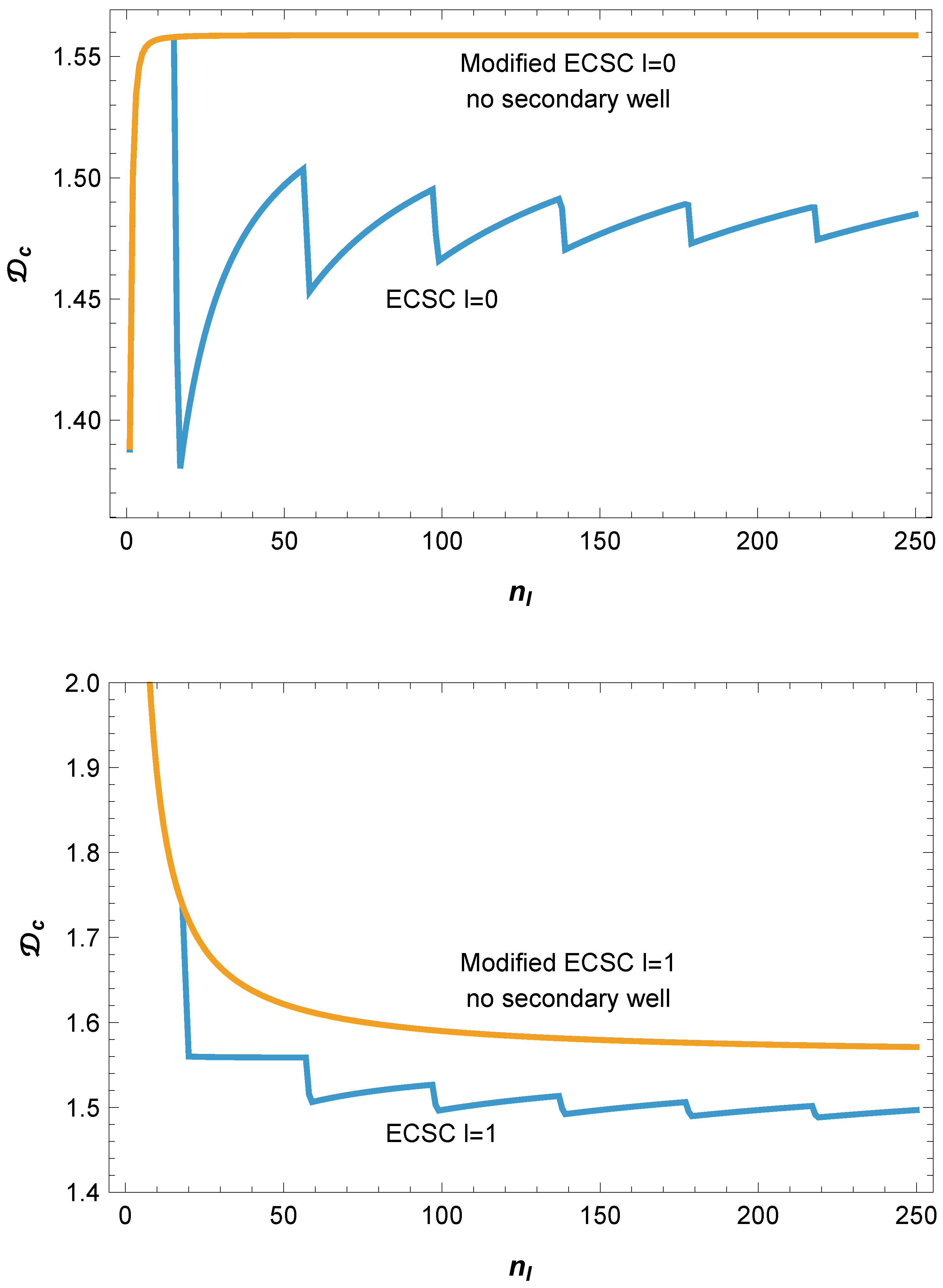
Figure 4.
vs n for ECSC l=0 potential with well depths increased by well scale factors of . The well depth reduces the period approximately as
Figure 4.
vs n for ECSC l=0 potential with well depths increased by well scale factors of . The well depth reduces the period approximately as
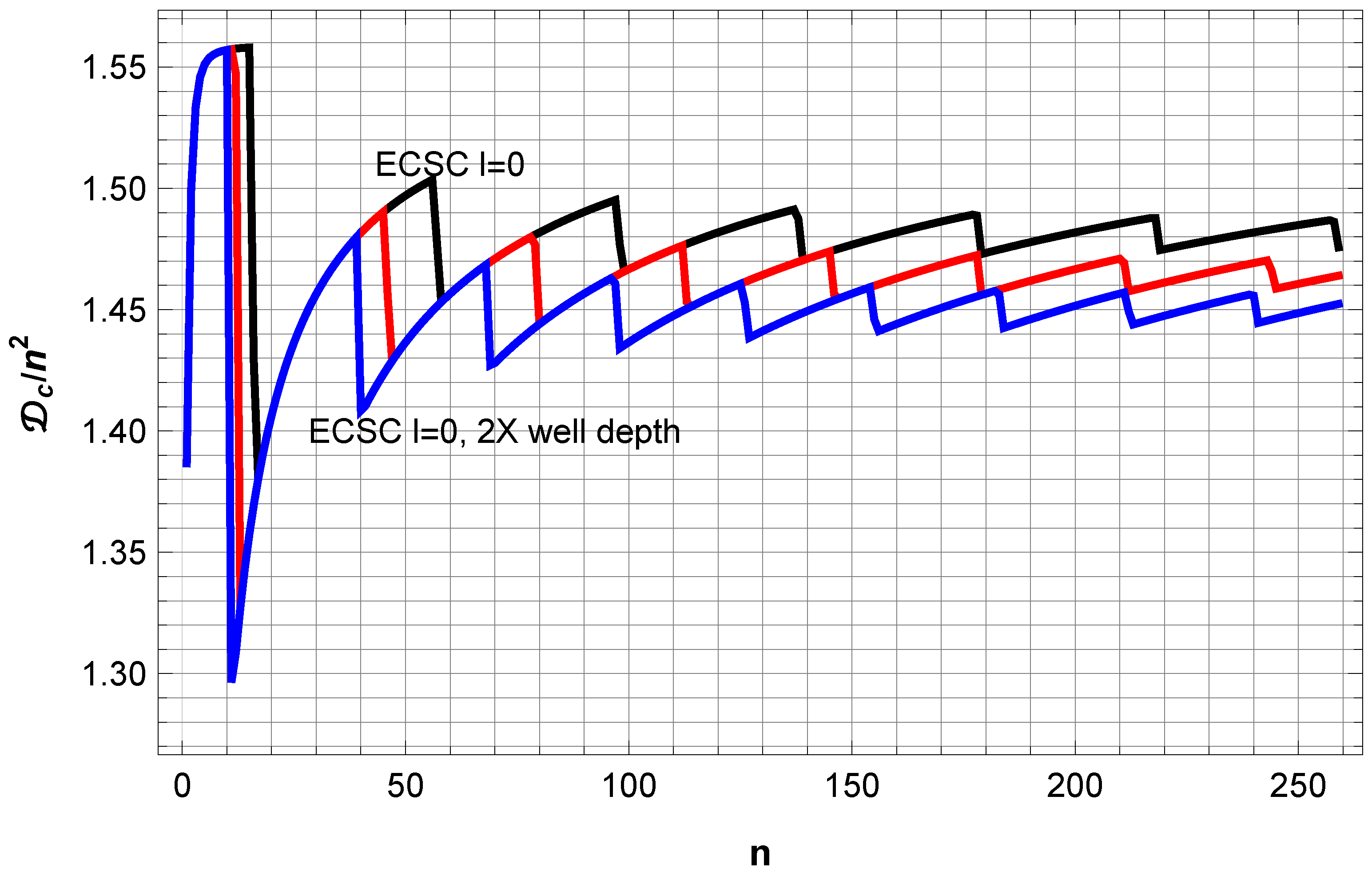
Figure 5.
vs n for ECSC l=0 potential with barrier height between primary and secondary wells () changed by barrier scale factors of . Reducing the barrier height lowers the n of first onset of the sawtooth structure, but does not appreciably change its period. In this plot the range of n is reduced to better show the displacements between the curves.
Figure 5.
vs n for ECSC l=0 potential with barrier height between primary and secondary wells () changed by barrier scale factors of . Reducing the barrier height lowers the n of first onset of the sawtooth structure, but does not appreciably change its period. In this plot the range of n is reduced to better show the displacements between the curves.
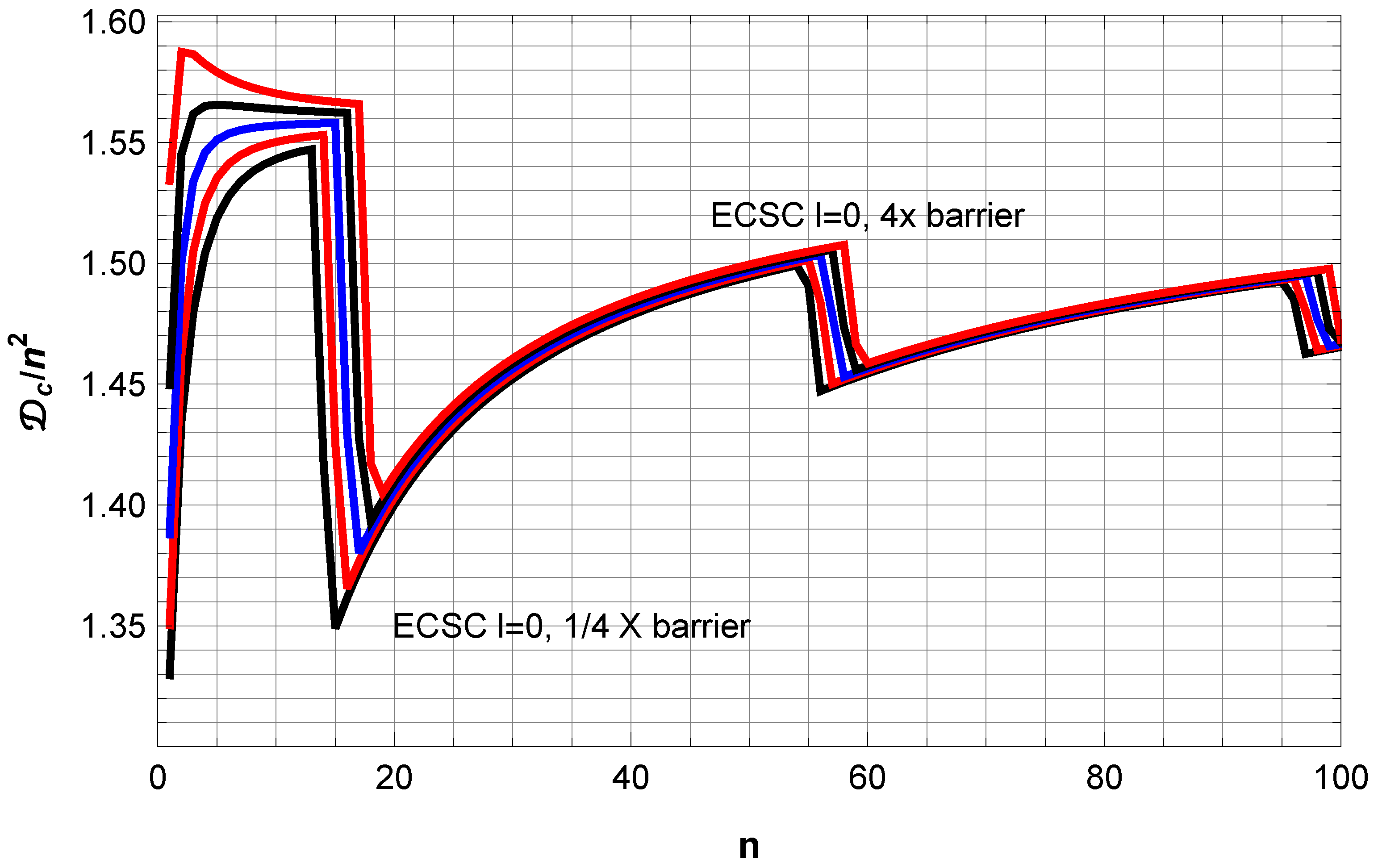
Figure 6.
vs n (red curve) theoretically calculated using neoclassical phase space quantization, with nominal values neoclassical parameters (, ) for comparison. These are intentional small deviations from canonical semiclassical values (0, 1/2) as described in the text. The PM-computed (essentially exact) result is shown in Blue. Agreement could be improved by allowing and to be functions of n, but for simplicity here we take them as constants. Our purpose is to show the basic origin of the sawtooth structure.
Figure 6.
vs n (red curve) theoretically calculated using neoclassical phase space quantization, with nominal values neoclassical parameters (, ) for comparison. These are intentional small deviations from canonical semiclassical values (0, 1/2) as described in the text. The PM-computed (essentially exact) result is shown in Blue. Agreement could be improved by allowing and to be functions of n, but for simplicity here we take them as constants. Our purpose is to show the basic origin of the sawtooth structure.
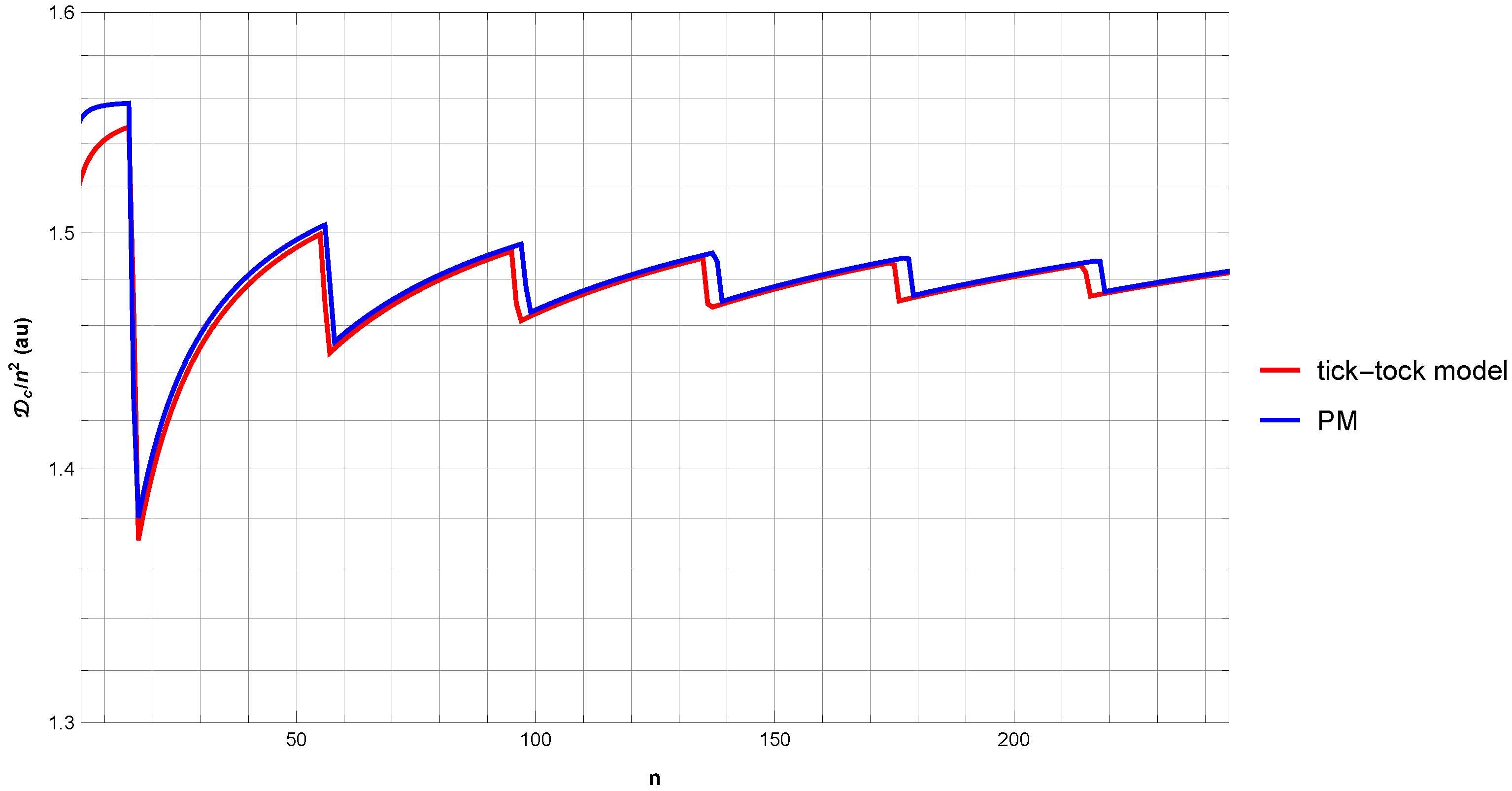
Figure 7.
vs n (red curve) for the ECSC potential with , calculated by PM (accurate to 30 digits) up to au. Note the sudden downward jump at around , which corresponds to the first bound state in the tertiary well at au. The upper plot shows the full range, while the lower figure shows a narrower range around this transition. This is in excellent agreement with the value predicted in advance by the simple neoclassical expression (for ) where and , and here (tertiary well) and (first bound state). It is also in agreement with more-accurate values from numerical phase space integrals.
Figure 7.
vs n (red curve) for the ECSC potential with , calculated by PM (accurate to 30 digits) up to au. Note the sudden downward jump at around , which corresponds to the first bound state in the tertiary well at au. The upper plot shows the full range, while the lower figure shows a narrower range around this transition. This is in excellent agreement with the value predicted in advance by the simple neoclassical expression (for ) where and , and here (tertiary well) and (first bound state). It is also in agreement with more-accurate values from numerical phase space integrals.
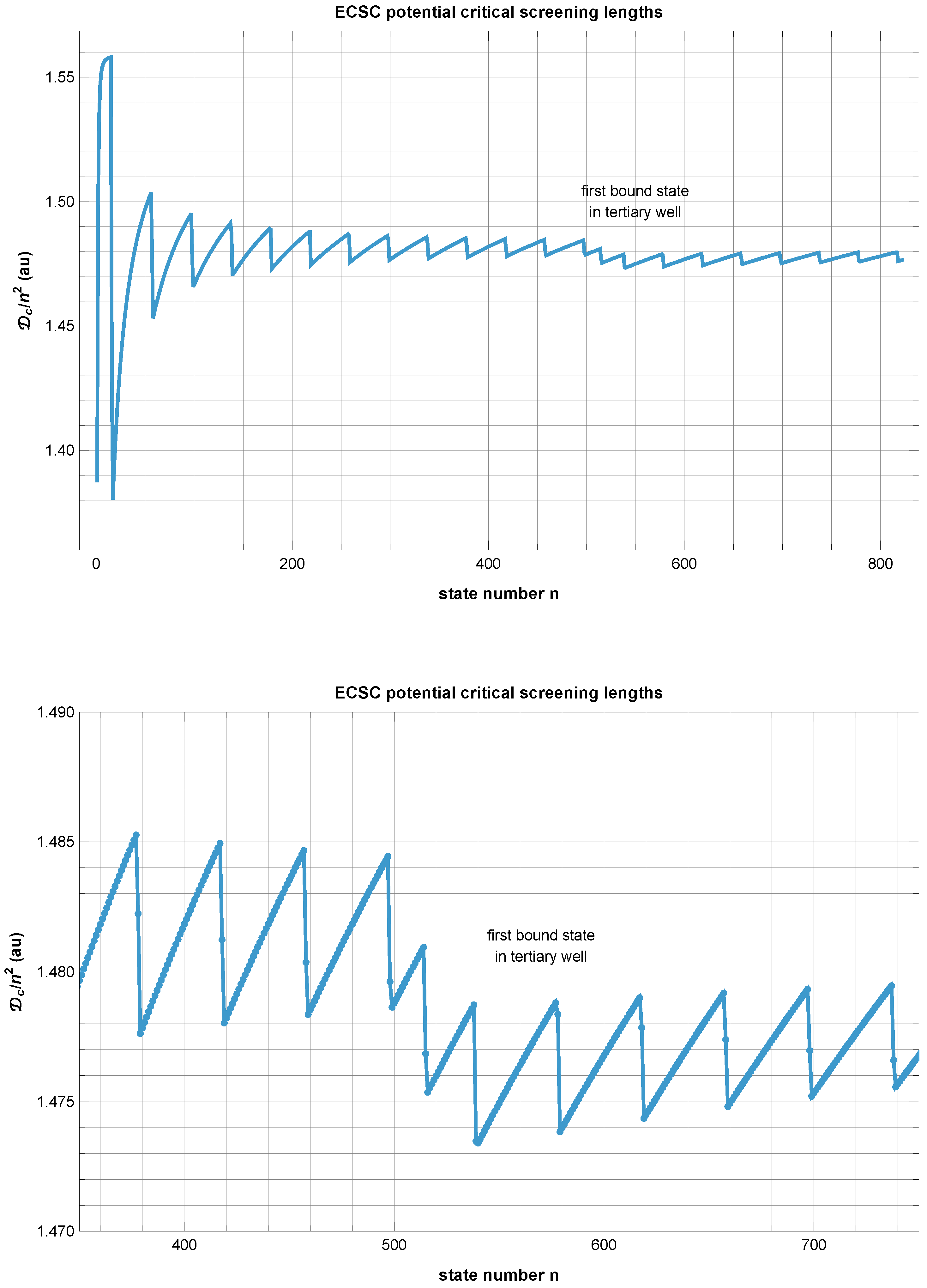
Figure 8.
ECSC neoclassically-estimated critical for states for the upper wells (secondary: , tertiary: , ...) residing between . The values shown were calculated by numerical integration of the phase space integrals, followed by neoclassical quantization condition. Similarly accurate results can be obtained from the simple formula, with small adjustments to the shape factors c (for the higher wells ). The manifolds corresponding to different wells (m) overlap above which will affect interpretation of spectra at macroscopic length scales. The (, ) state is responsible for the dip highlighted in Figure 15.
Figure 8.
ECSC neoclassically-estimated critical for states for the upper wells (secondary: , tertiary: , ...) residing between . The values shown were calculated by numerical integration of the phase space integrals, followed by neoclassical quantization condition. Similarly accurate results can be obtained from the simple formula, with small adjustments to the shape factors c (for the higher wells ). The manifolds corresponding to different wells (m) overlap above which will affect interpretation of spectra at macroscopic length scales. The (, ) state is responsible for the dip highlighted in Figure 15.
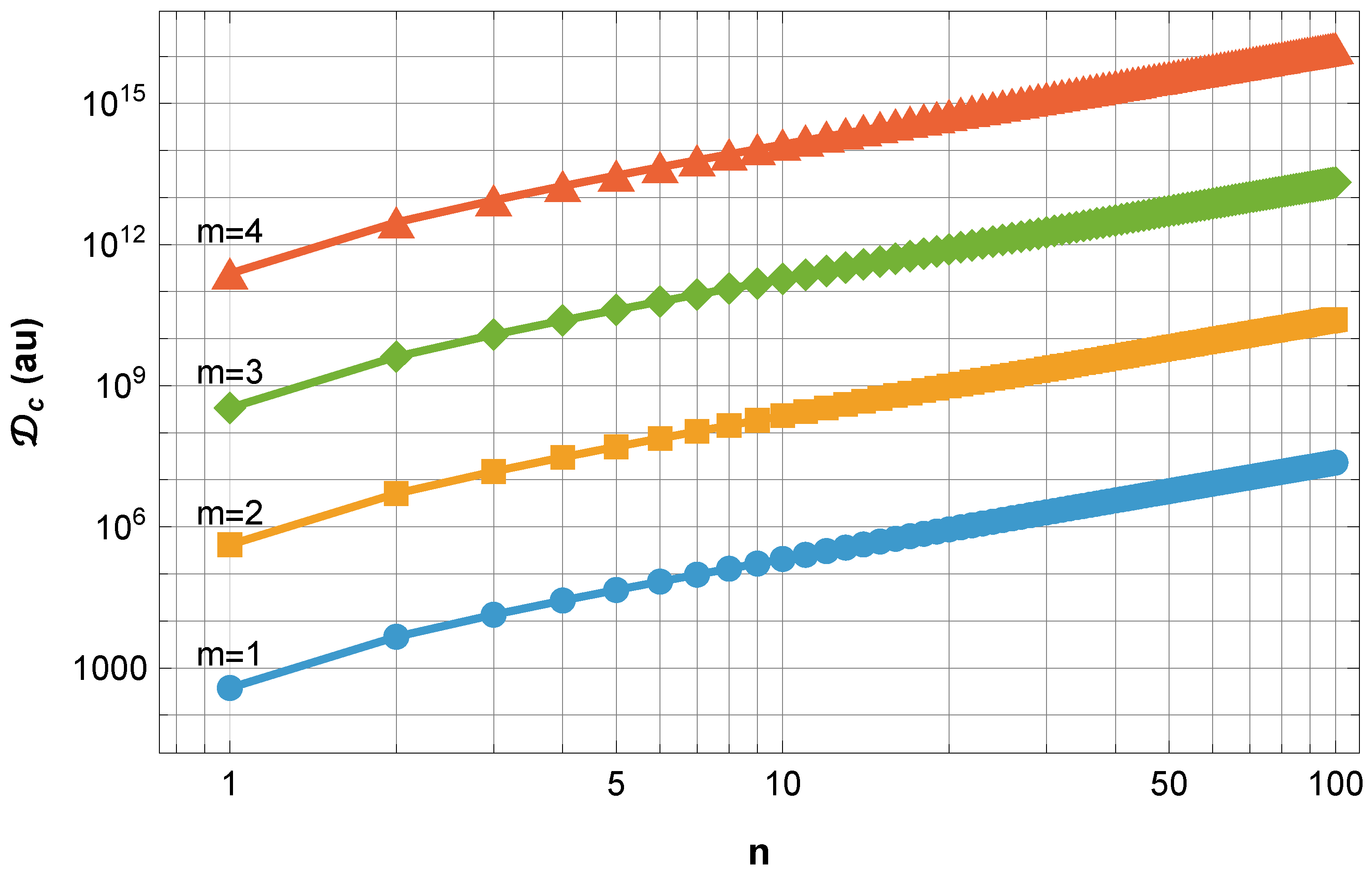
Figure 9.
Asymmetric quartic double-well potential is shown. The right panel shows is a plot of the phase space accessible at . The left (right) region corresponds to the left (right) well. is the momentum.
Figure 9.
Asymmetric quartic double-well potential is shown. The right panel shows is a plot of the phase space accessible at . The left (right) region corresponds to the left (right) well. is the momentum.
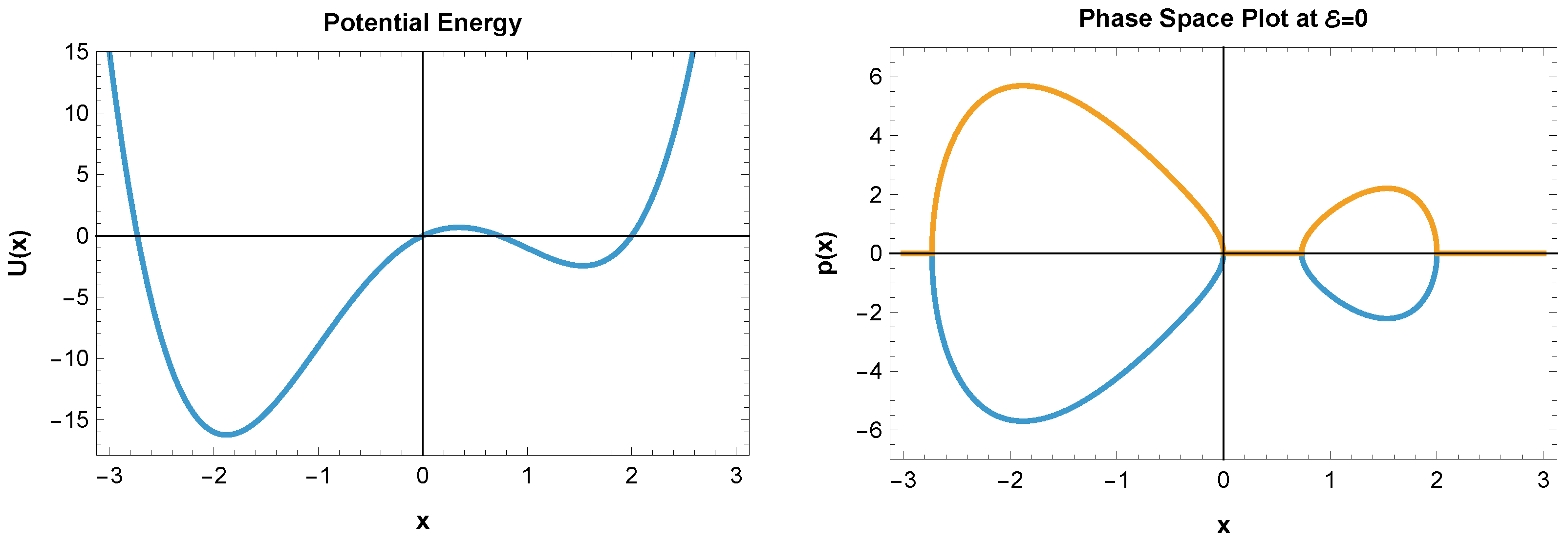
Figure 14.
vs and n for (from top): Hulthén, Yukawa, and ECSC potentials. Note the near-constant density of states vs l and n which extends indefinitely in both n and l (modulo tick-tock glitches). As the threshold is varied, the number of states is proportional to the shaded area, which grows as . This explains the linearity seen by Rogers et al Figure 5 and Lam and Varshni Figure 2, as well as our extensions to them.
Figure 14.
vs and n for (from top): Hulthén, Yukawa, and ECSC potentials. Note the near-constant density of states vs l and n which extends indefinitely in both n and l (modulo tick-tock glitches). As the threshold is varied, the number of states is proportional to the shaded area, which grows as . This explains the linearity seen by Rogers et al Figure 5 and Lam and Varshni Figure 2, as well as our extensions to them.
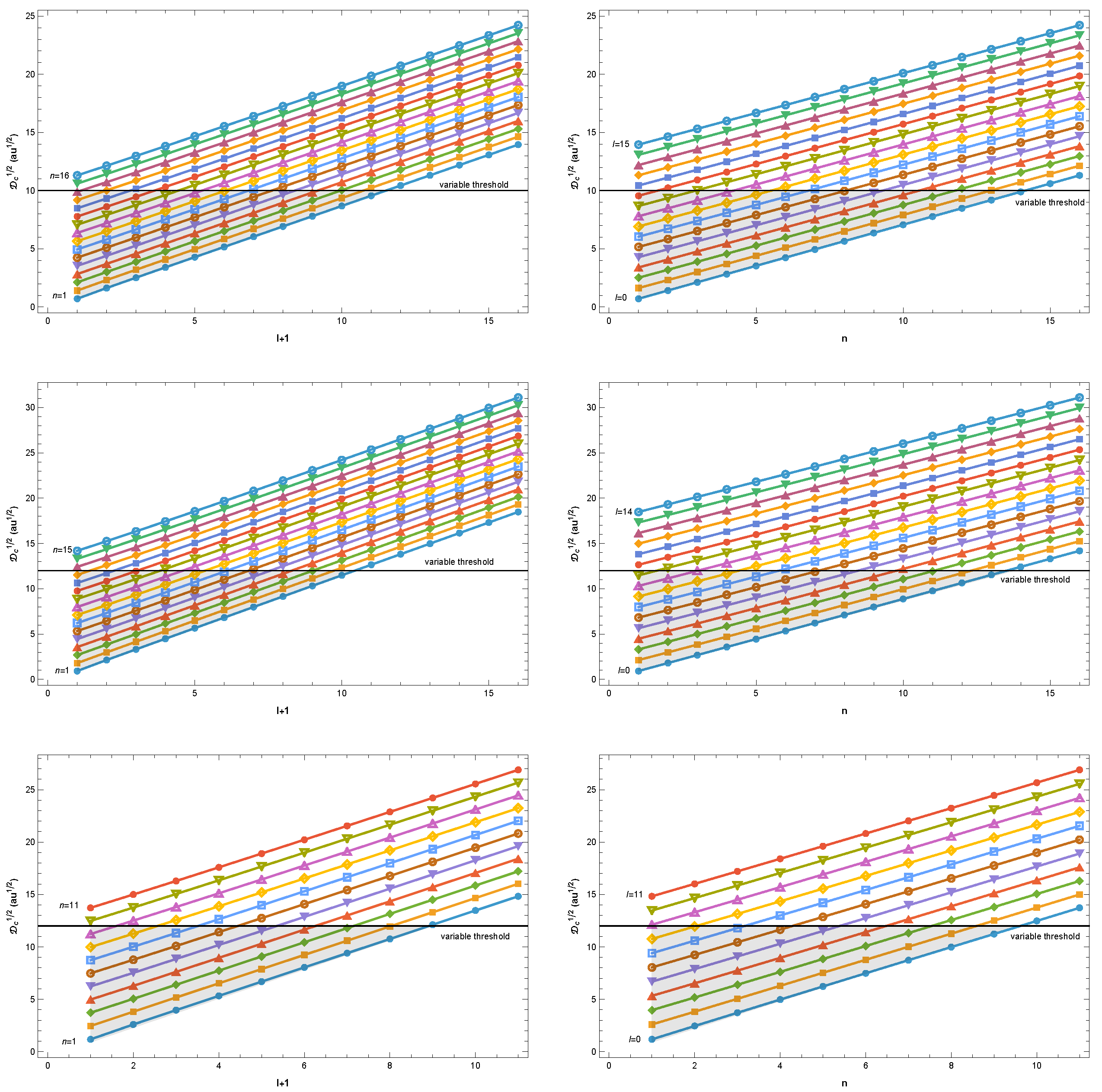
Figure 15.
vs and l. The average density of states is approximately constant in this representation also, extending indefinitely in n and l (modulo tick-tock glitches). The lowest state is 1s, the second pair is 2s, 2p, etc. Note the tick-tock glitch at for ECSC potential.
Figure 15.
vs and l. The average density of states is approximately constant in this representation also, extending indefinitely in n and l (modulo tick-tock glitches). The lowest state is 1s, the second pair is 2s, 2p, etc. Note the tick-tock glitch at for ECSC potential.
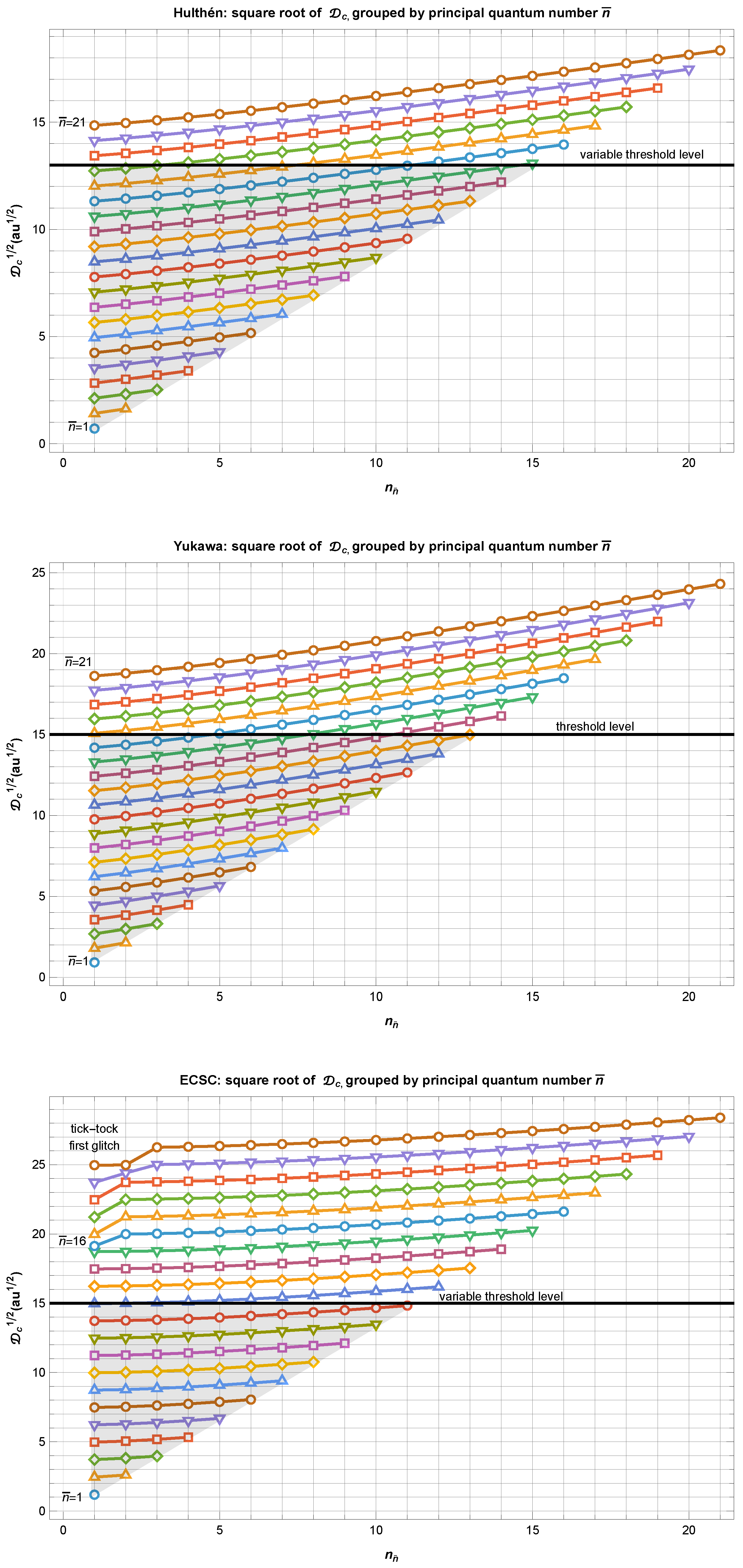
Figure 16.
Contour plot of vs and n, and residuals from bivariate linear fit to PM-calculated values computed to 30 digit accuracy. The nearly parallel and equally spaced contours indicate near-linearity.
Figure 16.
Contour plot of vs and n, and residuals from bivariate linear fit to PM-calculated values computed to 30 digit accuracy. The nearly parallel and equally spaced contours indicate near-linearity.
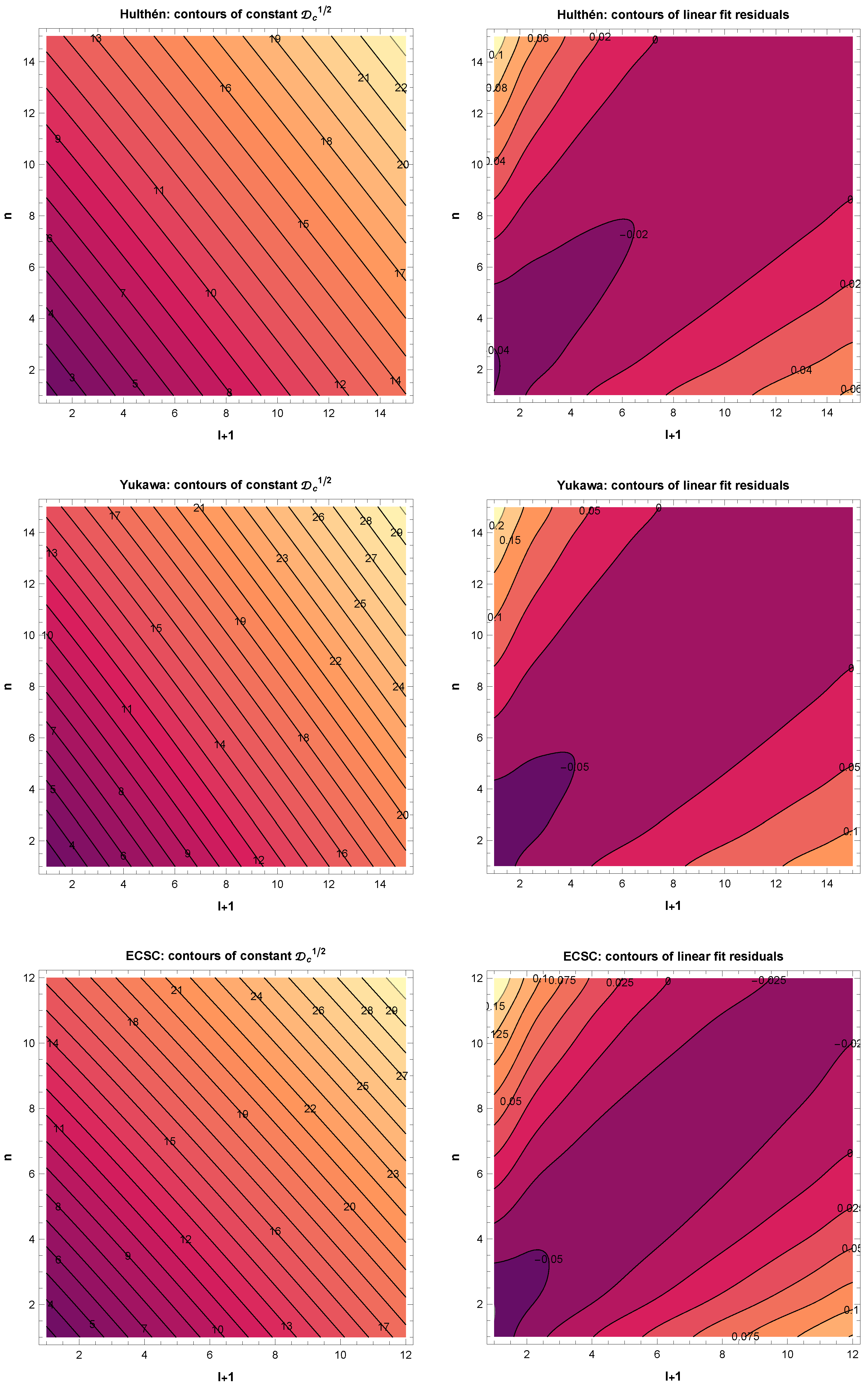
Figure 18.
Hyperbola or . All four quadrants are shown for context. The shaded region in the first quadrant is the physically relevant one that indicates the feasible range of q vs l, i.e. the range that might possibly bind states. The observed from linear fits in Table 2 is fairly close to the slope of the asymptote line, for Yukawa potential (as shown). Similar analysis applies to the other potentials.
Figure 18.
Hyperbola or . All four quadrants are shown for context. The shaded region in the first quadrant is the physically relevant one that indicates the feasible range of q vs l, i.e. the range that might possibly bind states. The observed from linear fits in Table 2 is fairly close to the slope of the asymptote line, for Yukawa potential (as shown). Similar analysis applies to the other potentials.
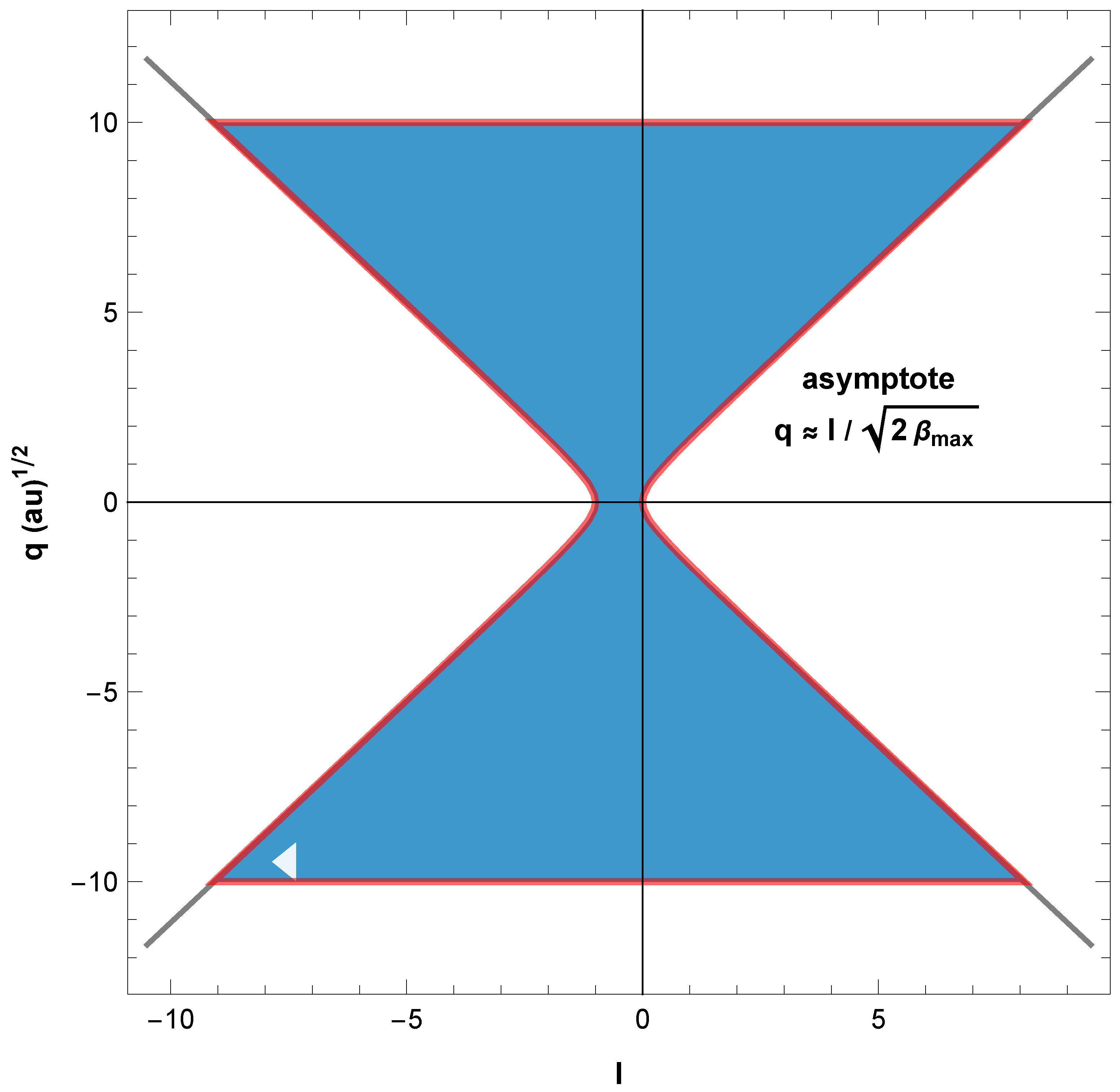
Disclaimer/Publisher’s Note: The statements, opinions and data contained in all publications are solely those of the individual author(s) and contributor(s) and not of MDPI and/or the editor(s). MDPI and/or the editor(s) disclaim responsibility for any injury to people or property resulting from any ideas, methods, instructions or products referred to in the content. |
© 2026 by the authors. Licensee MDPI, Basel, Switzerland. This article is an open access article distributed under the terms and conditions of the Creative Commons Attribution (CC BY) license (http://creativecommons.org/licenses/by/4.0/).
Copyright: This open access article is published under a Creative Commons CC BY 4.0 license, which permit the free download, distribution, and reuse, provided that the author and preprint are cited in any reuse.