

Submitted:
15 May 2026
Posted:
18 May 2026
You are already at the latest version
Abstract
Natural lateral particle segregation commonly occurs during the hydraulic deposition of slurry and thickened tailings in surface tailings storage facilities (TSFs), producing spatial heterogeneity in physical, hydrogeotechnical, and mineralogical properties, as well as in the water table. In sulfide-rich tailings, such heterogeneity complicates the design of reclamation cover systems, which are themselves affected by it. This study investigates the impact of physical and rheological properties of hard-rock mine tailings slurries on their segregation under hydrodynamic conditions. It proposes a multiparametric equation for the segregation index (SI) based on Buckingham's π-theorem. For this purpose, six flume experiments were conducted using tailings with initial solids mass concentrations of 63%, 66%, and 69% at slopes of 0.5% and 1%. Results revealed strong exponential correlations (R² > 0.95) between SI and tailings' physical properties (solids concentration, bulk density) as well as rheological parameters (Herschel–Bulkley yield stress and flow index, Cross infinite dynamic viscosity). The SI equation was developed using MATLAB nonlinear least-squares optimization with a trust-region reflective algorithm. Using an SI threshold of 0.05 to define non-segregating behavior, the proposed model can predict segregation tendencies as a function of tailings properties and slope conditions. Further laboratory and field investigations are needed to validate and generalize the criterion.
Keywords:
tailings
; flume test
; physical-rheological properties
; segregation index
; Buckingham π-theorem
; MATLAB
1. Introduction and Background
Lateral particle segregation is a phenomenon by which certain particles with similar properties tend to preferentially collect in one or another physical zone of an assembly. In the case of mine tailings, lateral particle segregation can occur when hydraulically discharged as a slurry in a tailings storage facility (TSF), creating a spatial distribution of the grain size distribution (GSD) as a function of distance from the discharge point. Three zones can then be distinguished: a beach zone with coarser particles near the discharge point, a decanting zone with finer particles, and a transition zone between the last two zones (MEND2001; Bussière 2007). In addition to GSD, segregation of slurry tailings can generate spatial heterogeneity in their physical properties (specific gravity Gs), GSD-controlled hydrogeotechnical properties (saturated hydraulic conductivity and the water retention capacity), and mineralogical properties.
In sulfide-rich tailings with high acid mine drainage (AMD) potential, this mineralogical lateral heterogeneity can also extend to the material’s reactivity and oxygen consumption capacity (Driouky et al. 2025). The design of efficient cover systems that act as oxygen and water barriers for the TSF reclamation becomes complex because it must consider the heterogeneities mentioned above (Bussière and Guittony 2020; Driouky et al. 2025). This design complexity could be alleviated by discharging non-segregating tailings, resulting in tailings properties that are relatively homogeneous throughout the TSF.
Achieving non-segregating tailings requires a comprehensive understanding of the primary factors governing particle size segregation during hydraulic deposition within TSFs. Generally, the mechanisms that govern the particle segregation process are still not well documented, owing to the complex nature of the phenomenon, where particle features (such as particle size and distribution, shape, and specific gravity), rheological behavior (non-Newtonian fluids), and hydrodynamic conditions (flow velocity) contribute to the complexity. Characterization of the rheological behavior of non-Newtonian fluids becomes then very important from an engineering perspective. Since the mid-1990s, Australian researchers have established relationships between solids mass concentration (= mass of solids/total mass) and tailings rheology (Pashias, 1996; Sofrá & Boger, 2011; Boger, 2012). Zhang et al. (2023) correlated particle-size distribution and solids mass concentration (Cw, 72–78%) with tailings rheology, demonstrating that the shear yield stress (ty) increases quadratically and the dynamic viscosity (h) increases linearly with Cw.
Flume tests are widely used for tailings beach slope prediction (e.g., Pirouz et al. 2005; Fitton 2007; Fourie & Gawu 2010; Nick 2013; Pirouz et al. 2013; Guang & Anstey 2015), segregation during tailings deposition (e.g., Pirouz et al. 2005; Mihiretu 2009; Fourie & Gawu 2010; Pirouz et al. 2013; Furtado et al. 2023), and yield stress estimation of non-Newtonian slurries (e.g., Gao & Fourie 2015). A summary of the flume characteristics, tested material, and principal results from a few studies is provided in the Appendix A. Tests were conducted with flumes of lengths 10, 12.2, and 20 m for 3, 1, and 1 channels, respectively; the remaining flumes were shorter than 10 m. The shortest length was 1.5 m.
The nearly one-dimensional segregation observed in short-length flume tests may not be representative of flow behavior in tailings storage facilities (TSFs). Unfortunately, few studies have evaluated the extent of in-situ segregation of flowing tailings. Maqsoud et al. (2015) investigated the rheological and hydrogeological behavior of flowing, thickened gold tailings (Cw-ini = 69%) using a field-scale experimental cell. The grain size distributions and rheological properties of the ten samples collected along the flow path were highly similar, indicating the absence of segregation and confirming homogeneous deposition. Rheological property analysis showed that the yield stress obtained using the Herschel–Bulkley model was approximately 8 Pa.
Despite these laboratory and field segregation studies, limited attention has been given to developing a predictive criterion for particle lateral segregation that considers both physical and rheological properties. However, in the case of vertical segregation simulated by static sedimentation tests, various researchers used a segregation index (SI) for this purpose (Chalaturnyk and Scott 2001; Mihiretu 2009). Chalaturnyk and Scott (2001) introduced the concepts of average solids mass concentration (Cw-avg) and segregation index (SI) to characterize this segregation boundary. Mihiretu (2009) proposed the segregation index SI defined with (Equation (1)) as a quantitative method for assessing particle segregation in static sedimentation tests.
where = sample height, = solids mass concentration of the sample section i, = average solids mass concentration of the samples.
Mihiretu (2009) suggested that the above-mentioned SI approach and criterion could also be applied to dynamic segregation evaluation (i.e., flume tests). In the case of a flume test, Equation (1) can be rewritten as follows:
where = length of section i along the flume (m), = solids content at the end of section i, = average solids content along the flume length.
Given that no unified model exists to predict particle segregation while accounting for all relevant physical and rheological factors, the objective of this paper is to develop preliminary uni- and multi-parametric non-segregation criteria for hard rock mine tailings slurries. Uni-parametric criteria are based on the relationships between the segregation index (SI) and the initial properties of the tailings. Furthermore, results obtained from flume tests and dimensional analysis using Buckingham’s π theorem are used to develop the multi-parametric criterion that includes rheological properties (shear yield stress and viscosity), solids content, and the flume slope and length.
2. Materials and Methods
2.1. Laboratory Flume Setup
Figure 1 shows the schematic drawing of the laboratory flume setup constructed to examine the depositional behavior of hard rock mine tailings. The flume consists of six sections, fabricated from polytetrafluoroethylene (PTFE), also known commercially as Teflon. Each section has a length (Li) of 2.44 m, resulting in a total flume length (Ltot) of 14.63 m. The internal dimensions of the channel are 0.52 m wide and 0.23 m deep.
The flume was assembled outside the laboratory, where the ground surface was not level. A metal support structure with height adjustment capability was used to stabilize the channel (Figure 2a). To achieve the target slope (0.5% or 1%) along the 14.63 m-long flume, the system first required precise leveling to a zero-slope using a Topcon RL-H4C laser level. The slope of the flume was then adjusted to the desired inclinations of (Figure 2b). Silicone sealant was applied along the joints between the flume panels to ensure watertightness and prevent leakage (Figure 2c), and leakage tests were performed by filling the flume with tap water.
2.2. Experimental Procedure and Program
The following steps were carried out before conducting the flume tests. The tailings received in 200-liter barrels were homogenized using a pump-mixer system (Figure 2d), with water added to achieve target initial solids mass contents (Cw) of 63%, 66%, and 69%. For this purpose, supernatant water was first carefully removed from the top of each barrel and transferred into buckets. Then, the highly concentrated tailings (Cw = 80%) were poured into a mixing pump chamber with the aid of a shovel. Due to the high initial solids content, supernatant water was gradually added until the mixture reached the target solids content Cw.
The amount of water required to achieve the desired solids mass concentration for each flume test was calculated using the following relationship:
where Mw_add is the mass of water to be added (kg), MTi is the initial total mass of tailings (kg), Cw-s the starting solids mass concentration (%), and Cw-f is the final solids mass concentration (%), with Cw-s > Cw-f.
The homogenization process lasted approximately 3 hours, ensuring a uniform mixture. Once homogenized, samples were taken to verify the target solids mass concentration. Then, the tailings were pumped from the mixing unit into a small upstream compartment and distributed across the full width of the flume (Figure 2e). For performing the flume test, four people were required to control the operating speed of the pumps, to hold the discharge tube to the flume (with an internal diameter of 38 mm), to take samples, and to keep the record of time for flow velocity (v) measurement, respectively. To calculate the flow velocity of the tailings along the flume, a time-of-arrival method was employed: the time at which the tailings reached the end of each flume section was recorded with a stopwatch. By calculating the time difference between the arrival of the tailings at consecutive sections, the average velocity (vm) within each section was determined by dividing the section length (2.44 m) by the corresponding travel time. The temperature (T°C) of the tailings was also continuously monitored along the flume using a thermocouple probe during the tests (see datalogger on Figure 2e). Tailings samples were collected at 2.44 m intervals along the flume (Figure 2f) for physical and rheological characterization. The number of samples collected depends on the distance the tailings travel. For example, with Cw-ini = 69%, the flow stopped at a distance L = 11.6 m. Figure 3 is an illustrative image of the flume test at the end of the flow test. After each test, the flume was cleaned thoroughly to prepare it for the next experimental run (Figure 2g).
Table 1 summarizes the experimental program and lists the properties of the tailing’s samples used for the six flume tests that were conducted at ambient air temperatures ranging between 21 and 23 °C.
2.3. Physical and Rheological Characterization of Tailings Samples Collected Along the Flume
Physical properties determined include the solids mass concentration, bulk density, specific gravity, and particle size distribution (PSD). The solids mass concentration, Cw, was derived from the water content (w) obtained after drying the samples in an oven at 70 °C until a constant dry mass was reached. The bulk or total density (ρ), specific gravity (Gs), and grain-size distribution were obtained using a mud balance (Metal Mud Balance, OFI Testing Equipment, USA), a helium pycnometer (Ultrapyc 1200e), and a laser particle size analyzer (Panalytical Mastersizer 3000), respectively. All these characterizations were realized in triplicate.
Rheological tests were conducted in triplicate using an AR2000 rheometer (TA Instruments, New Castle, DE, USA) with a vane geometry (rotor) measuring 28 mm in diameter and 42 mm in length. The vane was immersed in a cylindrical container (stator) (30 mm in internal diameter and 79 mm in height), with a lateral gap of 1 mm and a bottom gap of 4 mm (Figure 4). Before testing, instrument inertia was calibrated, temperature was maintained at 21 °C with the help of a Peltier temperature control system, and sample density was used to prepare the required 28.72 ml of slurry. Controlled shear rate tests were performed by applying a steady-state flow step procedure over shear rates () ranging from 0.1 to 100 s⁻¹ (upward ramp) and from 100 to 0.1 s⁻¹ (downward ramp) and measuring the shear stress (τ).
Experimental data consisted in rheograms (or flow curves) τ() and dynamic viscosity curves η(, where η = τ/. These curves were subsequently fitted with rheological models available in the analysis software (Rheology Advantage). For adjusting the flow curves, the Herschel-Bulkley’s generalized flow model (Equation (4)) was applied.
In this equation, τ is the shear stress (Pa), τ0-HB is the shear yield stress (Pa), i.e., the minimum stress to be applied to initiate flow, is the shear rate (1/s), is the flow index, and k is the consistency index (related to the viscosity of the fluid). Fluids exhibit a shear thinning behavior when n < 1, a shear thickening b when n > 1 and a Bingham behavior for n =1.
For analyzing the viscosity curves, the Cross rheological model was applied (Equation (5)):
where is the dynamic viscosity (Pa·s), is the dynamic viscosity at infinite or sufficiently high shear rate (Pa·s), is the initial dynamic viscosity (Pa·s), is a constant, and is the flow index specific to the Cross model.
The goodness of fit between the experimental and predicted curves was evaluated using the standard error (SE) (Equation (6)), which was calculated by the data analysis software through the least-squares method. According to the TA Instruments manual, the standard error is considered acceptable if it is less than 20 ‰.
where is the experimental value, is the value calculated by the rheological model, is the total number of measured data points, and Range is the difference between the maximum and minimum measured values.
3. Results
In the following, distributions of physical and rheological properties of the tailings along the flume length are presented. It is worth noting that the average flow velocity was 0.05 m/s, 0.03 m/s, and 0.02 m/s for Cw-ini = 63%, 66%, and 69%, respectively, in the flume with a 0.5% slope. For the flume with a slope of 1%, the average velocity was 0.1 m/s, 0.06 m/s, and 0.03 m/s for Cw-ini = 63%, 66%, and 69%. The average temperature of the tailings’ slurries ranged from 19 to 23 °C.
3.1. Distribution of Particle Size Distribution Along the Flume
Particle size distribution (PSD) curves with respect to the sampling distance (L) along the flume with a 1% slope are presented in Figure 5 for tailings with different solids contents (Cw-ini) of 63%, 66%, and 69%. The sample collected at a distance of 0 corresponds to the original tested tailings. By comparing the PSD curves along the flume, a noticeable difference in segregation behavior with respect to the solids content can be observed. At the highest tested Cw-ini of 69% (Figure 5a), the PSD curves at various distances nearly overlap, indicating a homogeneous and non-segregating flow where particles remain uniformly distributed along the flume. When the Cw-ini decreases to 66% (Figure 5b), slight divergence appears among the PSD curves, suggesting moderate segregation with coarser particles tending to settle near the upstream section. At a Cw-ini of 63% (Figure 5c), the variation between the PSD curves along the flume length becomes more pronounced, showing clearer particle-size separation along the flow path, where finer particles are transported further downstream. It should be mentioned that the variations of GSD along the flume with a slope of 0.5% (PSD not provided), for a given solid content, were less pronounced than those observed for a flume slope of 1%.
Figure 6a shows the variation in median particle size (D50, corresponding to 50% passing) along the flume length for different initial solids mass concentrations (Cw-ini = 63%, 66%, and 69%). In all cases, D50 decreases progressively with distance, indicating downstream particle segregation during slurry flow. The reduction is more pronounced at lower solids concentration (63%), whereas higher concentrations (69%) exhibit relatively smaller changes in D50, suggesting more homogeneous particle transport at higher solids contents. Figure 6b illustrates the variation of the fine particle fraction (P80µm) along the flume length for different initial solids mass concentrations (Cw-ini = 63%, 66%, and 69%). In all tests, P80µm increases progressively with distance, indicating downstream enrichment of fine particles due to segregation during slurry transport. The increase is most significant at the lowest solids concentration (63%), while higher concentrations show smaller variations, suggesting reduced segregation intensity and more uniform particle distribution at higher solids contents.
3.2. Distribution of Solids Content and Bulk Density Along the Flume
Figure 7 presents the variations of the solids content (Cw) and bulk density (ρ) along the flume for slopes of 0.5% and 1% (marks) together with the fitted linear trend curves (lines). It should be mentioned that these two parameters are interrelated and can be expressed through a mathematical relationship. As shown in Figure 7a,c, the solids mass concentration decreases progressively along the flume for all tests, with a steeper decline at lower initial Cw-ini.
At Cw-ini of 69%, the variation is minimal (0.32 for 0.5% slope and 0.27 for 1% slope), whereas at Cw-ini of 63%, the sharp reduction downstream (1.14 for 0.5% slope and 0.87 for 1% slope) reflects stronger particle segregation and dilution of the slurry. This trend shows that lower Cw-ini promotes higher segregation along the flow path. Based on Figure 7b,d, the bulk density (ρ) decreases gradually along with the flume for all Cw-ini, with the reduction becoming more pronounced at lower Cw-ini values. At Cw-ini = 69%, the bulk density remains nearly constant (variation of 0.005 for 0.5% slope and 0.003 for 1% slope), indicating limited segregation, whereas at Cw-ini = 63%, a sharp decline downstream (0.017 for 0.5% slope and from 0.015 for 1% slope) reflects significant particle separation and transport of finer and less dense material. Regarding the influence of the slope, Figure 7 and above given values for Cw and ρ at upstream and downstream of the flume indicate that the variation of CW and ρ with respect to the sampling distance along the flume is more pronounced for a 1% slope than for a 0.5% slope.
3.3. Distribution of Rheological Properties Along the Flume
Figure 8a,b display typical flow and viscosity curves obtained from the rheological tests (marks), together with the fitted curves based on the Herschel–Bulkley and Cross models (lines) for the flume test conducted with tailings at Cw-ini = 63% and slope of 0.5%. As shown in Figure 8a, the measured shear stress ranges from approximately 0.5 to 5.8 Pa over a shear rate range of 10 to 100 s⁻¹. The results show that shear stress decreases progressively with the sampling distance along the flume for a given shear rate. Indeed, near the discharge point (distance L = 0 m), shear stress values are the highest (2.0 Pa at 10 s⁻¹ and 5.8 Pa at 100 s⁻¹). As the flow advances downstream, shear stress drops significantly to around 0.5 Pa at 10 s⁻¹ and 1.0 Pa at 100 s⁻¹ at L = 14.63 m, reflecting particle segregation and increased water content. Based on Figure 8b, for Cw-ini = 63% with a flume slope of 0.5%, the viscosity consistently decreases with both increasing shear rate and sampling distance along the flume. Near the discharge point (L = 0 m), the viscosity values range from approximately 0.20 Pa.s at ~10 s⁻¹ to about 0.05 Pa.s at 100 s⁻¹. Farther downstream (L = 14.63 m), viscosity drops to approximately 0.03 Pa.s at ~10 s⁻¹ to about 0.01 Pa.s at ~100 s, indicating a more diluted and less resistant flow due to particle segregation and water enrichment along the flume. The flow and viscosity curves were fitted using the Herschel-Bulkley and Cross rheological models, respectively (see the lines in Figure 8).
Figure 9 presents the boxplots of triplicate rheological test results along the sampling distance at a 0.5% slope, showing the minimum and maximum values, the 25th and 75th percentiles, with the median line splitting them, and the mean values of the shear yield stress from the Herschel–Bulkley model and the dynamic viscosity at infinite (or sufficiently high) shear rate from the Cross model. For all cases, both shear yield stress and viscosity decrease exponentially with increasing sampling distance, indicating a clear reduction in rheological resistance downstream. At higher solids concentration (Cw-ini = 69%), average shear yield stress values are the largest (around 9 Pa near L = 0 m, decreasing to ~2.5 Pa at L = 14.63 m) and the average viscosity η∞ drops from ~0.14 Pa.s to ~0.05 Pa.s. Conversely, at lower solids concentration (Cw-ini = 63%), the average shear yield stress decreases gradually from ~2 Pa to ~0.25 Pa, and the average viscosity η∞ drops from ~0.04 Pa.s to ~0.01 Pa.s.
Figure 10 presents the boxplot of triplicate rheological test results along the sampling distance for 1% slope, showing the minimum, maximum, and mean values of the shear yield stress from the Herschel–Bulkley model, as well as the dynamic viscosity at an infinite (or sufficiently high) shear rate from the Cross model.
For the three solids concentration values, both shear yield stress and viscosity decrease exponentially with sampling distance. The reduction is most pronounced for Cw-ini = 63%, where average shear yield stress decreases from about 1.47 Pa near the discharge point to below 0.21 Pa at the end of the flume, and average viscosity falls from roughly 0.03 Pa.s to 0.01 Pa.s. In contrast, for Cw-ini = 69%, both parameters remain higher (average shear yield stress decreases from 7.32 Pa to 1.97 Pa; average viscosity decreases from 0.13 Pa.s to 0.03 Pa.s).
4. Development of Precursory Non-Segregation Criteria
Uni- and multi-parametric non-segregation criteria are proposed in the following. Uni-parametric criteria represent the threshold values of each initial physical and rheological property of the tailings above which segregation does not occur. In contrast, the multi-parametric criterion combines all these properties into a single equation.
4.1. Uni-Parametric Non-Segregation Threshold Limits
Figure 11 illustrates the relationship between the segregation index (SI) calculated using Equation (2) for the two flume slopes (0.5% and 1%) and various physical and rheological parameters of the tailings. In all cases, the segregation index (SI) decreases exponentially with increasing values of the studied parameters (the initial solids mass concentration (Cw-ini), bulk density (ρ ini), Herschel-Bulkley shear yield stress (τ0-HB-ini), infinite dynamic viscosity (η∞-ini)). The exponential fittings achieved coefficients of determination () greater than 0.95 in all cases (equations not shown), confirming the strong predictive correlation between SI and the examined physical and rheological parameters.
The dashed line represents the approximate threshold between segregating and non-segregating behavior (SI = 0.05). Based on the results presented in this figure, segregation threshold limits can be determined for each parameter. These threshold values define the parameter ranges beyond which segregation no longer occurs. These limits may be identified graphically by locating the intersection between the curve corresponding to SI = 0.05 and the function SI = f (studied parameter).
For the slope of 0.5%, the tailings tested would be non-segregating when the initial solids mass concentration (Cw-ini), bulk density (ρ ini), Herschel-Bulkley shear yield stress (τ0-HB-ini), infinite dynamic viscosity (η∞-ini) is approximately higher than 63% (Figure 11a), 1.68 g/cm3 (Figure 11b), 2.0 Pa (Figure 11c), 0.04 Pa.s (Figure 11d), respectively. For a slope of 1%, the tailings tested would be non-segregating across all tested solid contents.
Since segregation depends not only on the solids concentration but also on rheological properties and hydrodynamic conditions, single-parameter criteria are inherently specific to a given tailings and therefore cannot be considered universally applicable segregation criteria. A multi-parameter criterion, such as the one developed below, would provide a more robust and generalized framework for assessing segregation behavior.
4.2. Multiparametric Non-Segregation Threshold Limit
To develop the non-segregation criterion based on physical and rheological properties, dimensional analysis involving Buckingham’s π-theorem was used. Different authors present applications of the π-theorem to various fluid mechanics and heat/mass transfer problems. It provides a systematic method for reducing the number of variables in a problem by grouping them into dimensionless parameters (Buckingham, 1914; Sofra, 2001; Sofra & Boger, 2002; Yarin, 2012; Gao, 2015; Dumka et al., 2022; Shaikhli et al., 2024).
In this study, an empirical model was developed using the Buckingham π-theorem to evaluate the influence of both rheological and physical properties on the segregation index (SI). The model demonstrates multiparametric nonlinear behavior and was solved in MATLAB using the trust-region reflective algorithm, a robust iterative optimization technique for nonlinear least-squares problems. In this framework, the objective is to minimize the following function:
where = observed segregation index, = model prediction for given input and coefficients are unknown coefficients to be determined. The subscript represents the observation number or data point in the dataset, and N is the total number of data points.
The following six steps are considered to obtain based on the Buckingham’s π-theorem.
Step 1: The independent variables involved in the problem and their dimensions are determined (see Table 2). Here, the total number of variables (n) is 7. The solids content (Cw) is not considered an independent variable, as it is directly dependent on density (ρ) already included in the 7 variables.
Step 2: The fundamental dimensions governing the physical system are identified. The selected dimensions are mass (M), length (L), and time (T), which are sufficient to represent all physical quantities involved in the analysis. The number of fundamental dimensions k is 3.
Step 3: The total number of dimensionless groups according to the Buckingham π-theorem is determined as:
Step 4: The repeating variables that must collectively represent all the fundamental dimensions (M, L, T) are selected. This selection is not necessarily unique, as different researchers may choose different sets of repeating variables. Consequently, the resulting π-terms are also not unique. The methodology recommends selecting a suitable combination of variables, typically including one geometric variable, one kinematic variable, and one fluid property, as is common in fluid mechanics problems. In this study, the repeating variables chosen for each -group are:
Step 5: The π-groups are constructed by combining the selected repeating variables with the remaining variables to form dimensionless groups, as illustrated in Table 3. Each π-group represents a unique combination that captures the relationship among the physical parameters governing the system.
Step 6: The final dimensionless relationship is established by combining the constructed π-groups. The relationship can be expressed as follows:
or:
The proposed multi-parametric segregation model for predicting the segregation index (SI) based solely on the initial physical and rheological parameters of the mine tailings and the flume slope is given as follows:
For the mine tailings used in this paper, β = 7.77629e-07 (physico-rheological weighting factor), a = 0.613127(rheological factor), b = 8.77633(flow index factor), and c = 0.38665(slope factor).
Table 4 presents the physico-rheological properties of the tailings used to calculate the segregation index (SI) and compares the calculated and experimental SI values. Each row in the table represents a single flume test. The columns list the corresponding initial physical and rheological properties. Figure 12 illustrates the correlation between the experimental segregation index (SI-Experiment) and the modeled segregation index (SI-Model). The low root mean square error (RMSE = 0.003) and (R2=0.96) indicate a strong agreement between the two.
where SIExp = segregation index obtained from experimental measurements, SIModel = segregation index predicted by the model, N = number of data points, and i = flume test number (1, 2, …, 6).
The authors are aware that this validation using dependent data (used to develop the model) is insufficient. Independent data obtained from other flume tests with different types of tailings will allow for validation of the model’s robustness.
This model, derived from a single tested material, remains preliminary. Indeed, it was expected that the segregation index (SI) would decrease with increasing yield stress; however, this trend is not observed according to Equation (10). The model will be improved using a larger dataset obtained from tailings with varying initial characteristics. It will then be extended to incorporate additional parameters such as grain-size distribution, specific gravity, and other relevant independent properties.
5. Conclusions
Flume experiments were conducted to investigate the depositional characteristics of hard-rock mine tailings slurries from a geotechnical perspective, focusing on how their physico-rheological properties evolved along a 14.63 m-long flow path. Tailings were sampled at 2.44 m intervals and tested using a laser diffraction particle size analyzer, a helium pycnometer, and an AR2000 rheometer to determine particle size distribution, solid grain density, and rheological properties. The solids content was obtained from the gravimetric water content.
The physical properties of samples collected along the flume showed a progressive decrease in solids concentration (Cw) and bulk density (ρ). Rheological parameters based on the Herschel–Bulkley and Cross models indicated a noticeable reduction in shear yield stress (τ0HB), and infinite-shear viscosity (), respectively. Overall, the segregation index (SI) was found to decrease exponentially with increasing Cw, ρ, τ0HB and η∞. Using a segregation index threshold of SI < 5% or 0.05 as criterium for non-segregating condition, the tested tailings displayed non-segregating behavior when Cw-ini, ρini, τ0-HB-ini or η∞-ini is approximately higher than 63%, 1.68 g/cm3, 2.0 Pa, or 0.04 Pa.s, respectively.
A fundamental dimensional analysis technique using the Buckingham π theorem enabled the development of a multiparametric segregation index model that integrates both physical and rheological tailings properties and the flume slope. The proposed model accurately predicts the segregation index (and, consequently, segregation behavior) using a SI threshold of 5%, achieving a high coefficient of determination (R² = 0.96) and a low RMSE (0.003) between experimental and modeled values. Further flume tests will be carried out soon with other types of tailings to validate the proposed model with independent data.
Author Contributions
Conceptualization, SMD, MM, TB, and AM.; methodology, SMD, MM, TB, and AM.; software, SMD.; validation, SMD, MM, TB, and AM.; formal analysis, SMD, MM, and TB.; investigation, SMD, MM, TB, ADD and OSD; resources, MM and TB.; data curation, SMD; writing—original draft preparation, SMD; writing—review and editing, SMD, MM, TB, AM, ADD and OSD.; visualization, SMD; supervision, MM, TB, and AM.; project administration, MM.; funding acquisition, MM and TB. All authors have read and agreed to the published version of the manuscript.
Funding
This research was funded by the NSERC Collaborative Research and Development (CRD) grants (grant number: RDCPJ518243-17) and the industrial Partners (Iamgold Corporation-Westwood Mine; and the Research Institute of Mines and Environment RIME UQAT-Polytechnique).
Acknowledgments
The authors would like to thank the URSTM research professionals (Akué-Sylvette Awoh and Hadj Ghani Menasria) and the entire technical team (particularly Joël Beauregard, Raphaël Chartier, Alain Perreault, and Ibrahima Hane) for their support in performing the laboratory work.
Conflicts of Interest
The authors declare no conflict of interest. The funders had no role in the design of the study; in the collection, analyses, or interpretation of data; in the writing of the manuscript; or in the decision to publish the results.
Appendix A.

Table A1.
Summary of a few flume tests on mine tailings.
| Reference | Flume Length (m) | Flume Width (m) | Flume Depth (m) | Materials | Cw (%) | Goal of the study | General results |
|---|---|---|---|---|---|---|---|
| Blight et al. (1985) | 1.8 | 0.3 | 0.6 | Silty tailings | 50-70 | Determining beach profile. | Final normalized profile for each test. |
| Lighthall (1987) | 2 | 1.5 | 0.15 | Tailings from a copper and zinc mine | 20-45 | Assessing tailings beach slopes for Dam design. | Steeper laboratory slopes than field slopes. |
| Boldt (1988) | 12.2 | 0.6 | 0.6 | Fine mill tailings from a copper- silver mine |
20-57 | Examining tailings beach formation, shear strength, permeability, and grain size distribution. | Average slope, shear strength, and permeability tests. |
| Fourie (1988) | 2 – 4 | 0.6 | 0.6 | Bauxite, nickel ore slurry, coal tailings | - | Examine the beaching and permeability of bauxite, nickel, and coal tailings. | Non-segregating slurries behaved as viscous fluids, different from sand-based segregating tests. |
| Pirouz et al. (2005) | 10 | 1 | 0.5 | Gold mine tailings | 54-59 | Investigate the beach formation slope. | Overall, the beach slope is governed by the equilibrium slope of self-formed turbulent channels. |
| Fitton et al. (2006), Fitton (2007) | 10 | 0.15 | 0.5 | Gold mine tailings | 44-60 | Prediction of beach slope. | Developed a new semi-empirical model for beach slope prediction. |
| Mihiretu (2009) | 2.44 | 0.11 | 0.5 | Oil sand tailings | 55-57 | Study dynamic segregation under zero, 5%, and 10% slopes for sand–kaolinite mixtures (SFR = 1, 2, and 4). | The beach profile steepness increased with Cw. Increasing SFR increased segregation. |
| Henriquez & Simms (2009) | 2.5 | 0.15 | 0.3 | Gold mine tailings | 40-70 | Compare the dynamic vs the steady-state deposition of the tailings stack. | Angle of a tailings deposit at steady-state is dependent on the scale of the flow. |
| Fourie et al. (2010) | 1.8 | 0.15 | 0.5 | Zinc, gold, and copper tailings | 55-59 | Beach slope prediction considering the wall friction of the flume. | A steeper slope angle than the field observation. |
Table A2.
Summary of a few flume tests on mine tailings (ctd.).
| Reference | Flume Length (m) | Flume Width (m) | Flume Depth (m) | Materials | Cw (%) | Goal of the study | General results |
|---|---|---|---|---|---|---|---|
| Mizani et al. (2010) | 2.43 | 0.15 | 0.3 | Gold mine tailings | 68-75 | How settling and capillary action change the rheology of overland flow and deposition geometry. | The tailings exhibited consistently higher yield stresses with longer deposition times. |
| Nik (2013) | 2.38 | 0.18 | 1 | Oil sand tailings | 37-65 | Quantifying segregation index (SI) based on flume profiles | Increasing CW and yield stress led to shorter flow distances and steeper slopes. |
| Pirouz et al. (2013) | 10 | 1 | 0.5 | Copper mine tailing | 56-72 | Beach slope prediction | Slope value is a complex function of rheology, solid content, PSD, etc. |
| Gao & Fourie (2015) | 2.5 | 0.2 | 2.5 | Mixtures of kaolin clay and water | - | Evaluating the influence of yield stress and viscosity on flow profiles. | Increasing yield stress and viscosity led to shorter flow distances and steeper deposit profiles. |
| Guang & Anstey (2015). | 2.4 | 0.15 | 0.3 | fine tailings from two existing oil sands mines | 30-40 | prediction of field-scale tailings beach slopes by BSLOPE | The ability to apply the BSLOPE model to the flume and full-scale deposits of polymer-treated MFT |
| Gao & Fourie (2019) | 1.5 | 0.2 | 0.1 | thickened tailings | - | Effect of yield stress and viscosity on the slope of deposited tailings by CFD simulation | The yield stress of the fluid generally has more influence on the final profiles than the viscosity. |
| Furtado et al. (2023) | 1.65 | 0.31 | 0.62 | Fine tailings from the niobium ore flotation process. | 57-69 | Evaluating the feasibility of non-segregable high-density tailings. | Particle-size curves along the flume overlapped, no segregation detected. |
| Li et al. (2024) | 20 | 2 | 1.2 | Iron tailings pond | 20-50 | Investigate the flow and depositional behavior of tailings slurry | Developed and validated an empirical beach slope equation for segregating tailings. |
References
- AMEC Environment; Infrastructure. Beach fine captures study; COSIA: Calgary, Alberta, 2013. [Google Scholar]
- Aubertin, M.; Bussière, B.; Chapuis, R. P. Hydraulic conductivity of homogenized tailings from hard rock mines. Canadian Geotechnical Journal 1996, 33(3), 470–482. [Google Scholar] [CrossRef]
- Blight, G.E.; Thomson, R.R.; Vorster, K. Profiles of hydraulic-fill tailings beaches, and seepage through hydraulically sorted tailings. Journal of the South African Institute of Mining and Metallurgy 1985, Vol. 85(N0. 5), 157–161. [Google Scholar]
- Boger, D.V. Personal perspective on paste and thickened tailings: a decade on. Mining Technology, Transactions of the Institutions of Mining and Metallurgy: Section A 2012, 121:1, 29–36. [Google Scholar] [CrossRef]
- Boldt, CMK. Report of Investigation: Beach characteristics of mine waste tailings; U.S. Bureau of Mines Report: Washington D.C, 1988. [Google Scholar]
- Buckingham, E. On physically similar systems: Illustrations of the use of dimensional equations. Physical Review 1914, 4, 345–376. [Google Scholar] [CrossRef]
- Bussière, B. Hydrogeotechnical properties of hard rock tailings from metal mines and emerging geoenvironmental disposal approaches. Canadian Geotechnical Journal 2007, 44(9), 1019–1052. [Google Scholar] [CrossRef]
- Hard rock mine reclamation: From prediction to management of acid mine drainage, 1st ed.; Bussière, B., Guittonny, M., Eds.; CRC Press, 2020. [Google Scholar] [CrossRef]
- Chalaturnyk, R. J.; Scott, J. D. Soil structure behaviour diagram. High Density and Paste Tailings 2001; 2001. [Google Scholar]
- De Groot, M.B.; Heezen, F.T.; Mastbergen, D.R.; Stefess, H. Slopes and density of hydraulically placed sands. In Hydraulic Fill Structures; ASCE Geotechnical Special Publication 21, 1988. [Google Scholar]
- Donahue, R.; Sego, D.; Burk, B.; Krahn, A.; Kung, J.; Islam, N. Impact of ion exchange properties on the sedimentation properties of oil sands mature fine tailings and synthetic clay slurries. In Proceedings of the First International Oil Sands Tailings Conference, Edmonton, Alberta, Canada; 2008. [Google Scholar]
- Driouky, Z.; Mbonimpa, M.; Temgoua, M.D; Demers, I.; Belem, T. Lateral segregation-induced distribution of sulfide tailings reactivity with oxygen in a tailings storage facility. MEDGU 2025 - 5th Mediterranean Geosciences Union, Athens, Greece, 10–12 November; 2025. [Google Scholar]
- Dumka, P.; Chauhan, R.; Singh, A.; Singh, G.; Mishra, D. Implementation of Buckingham’s Pi theorem using Python. Advances in Engineering Software 2022, 173, 103232. [Google Scholar] [CrossRef]
- Fitton, T. G.; Chryss, A. G.; Bhattacharya, S. N. Tailings beach slope prediction: a new rheological method. International Journal of Mining, Reclamation and Environment 2006, 20(3), 181–202. [Google Scholar] [CrossRef]
- Fitton, T. Tailings beach slope prediction. Doctoral dissertation, RMIT University, 2007. [Google Scholar]
- Fourie, AB. Beaching and permeability properties of tailings. In Hydraulic Fill structures, ASCE ceotechnical special publication 21; American Society of Civil Engineers: New York, 1988; pp. 142–154. [Google Scholar]
- Fourie, AB; Gawu, SKY. The validity of laboratory flume data for predicting beach slopes of thickened tailings deposits. In Paste 2010: Proceedings of the Thirteenth International Seminar on Paste and Thickened Tailings; Jewell, R, Fourie, AB, Eds.; Australian Centre for Geomechanics: Perth, 2010; pp. 241–253. [Google Scholar]
- Fourie, AB; Gawu, SKY. The validity of laboratory flume data for predicting beach slopes of thickened tailings deposits. In Paste 2010: Proceedings of the Thirteenth International Seminar on Paste and Thickened Tailings; Jewell, R, Fourie, AB, Eds.; Australian Centre for Geomechanics: Perth, 2010; pp. 241–253. [Google Scholar]
- Furtado, R. M.; Chaves, A. P.; Testa, F. G.; de Paula, P. T. Feasibility of high-density and non-segregable niobium ore tailings. Minerals 2023, 13(6), 820. [Google Scholar] [CrossRef]
- Gao, J.; Fourie, A. Using the flume test for yield stress measurement of thickened tailings. Minerals Engineering 2015, 81, 116–127. [Google Scholar] [CrossRef]
- Guang, R.; Anstey, D. Application of flume testing to field-scale beach slope prediction. 2015. [Google Scholar] [CrossRef]
- Henriquez, J.; Simms, P. Dynamic imaging and modeling of multilayer deposition of gold paste tailings. Minerals Engineering 2009, 22(2), 128–139. [Google Scholar] [CrossRef]
- Li, Q.; Duan, Z.; Shi, H.; Yu, Y.; Zhang, H.; Fu, B. Development of a full-scale flume test system for depositional behavior study of segregating tailings. Bulletin of Engineering Geology and the Environment 2024, 83(2). [Google Scholar] [CrossRef]
- Lighthall, Peter C. Innovative tailings disposal methods in Canada. International Journal of Surface Mining, Reclamation and Environment 1987, 1(1), 7–12. [Google Scholar] [CrossRef]
- Maqsoud, A.; Mbonimpa, M.; Bussière, B. Rheology and hydrogeological behavior of thickened tailings disposal using field experimental cell. 10th International Congress on Acid Rock Drainage and IMWA Annual Conference; 2015. [Google Scholar]
- MathWorks. MATLAB (Version R2025b); The MathWorks, Inc., 2025; Available online: https://www.mathworks.com.
- MEND. Manual report 5.4.2. In Summary, Volume 2: Sampling and Analysis, Volume 3: Prediction, Volume 4: Prevention and Control; Mineral and Energy Technology (CANMET): Ottawa, Ontario, Canada, 2001; Volume 1. [Google Scholar]
- Mihiretu, Y. T. Fundamentals of segregation. Ph.D. thesis, Department of Civil and Environmental Engineering, University of Alberta, 2009. [Google Scholar]
- Mizani, S. Rheology of thickened gold tailings for surface deposition. Master’s thesis, Carleton University, Ottawa, 2010. [Google Scholar]
- Nik, R. M. Application of dewatering technologies in production of robust non-segregating tailings. Ph.D. thesis, Department of Civil and Environmental Engineering, University of Alberta, 2013. [Google Scholar]
- Pashias, N. The characterization of bauxite residue suspensions in shear and compression. PhD thesis, The University of Melbourne, Melbourne, Australia, 1996. [Google Scholar]
- Pirouz, B.; Kavianpour, M. R.; Williams, P. Thickened tailings beach deposition: Field observations and full-scale flume testing. In 8th International Seminar on Paste and Thickened Tailings; Australian Centre for Geomechanics, 2005; pp. 53–72. [Google Scholar] [CrossRef]
- Pirouz, B.; Seddon, K.; Pavissich, C.; Williams, P.; Echevarria, J. Flow through tilt flume testing for beach slope evaluation at Chuquicamata Mine, Codelco, Chile; Proceedings of the 16th International Seminar on Paste and Thickened Tailings, Australian Centre for Geomechanics: Perth, 2013; pp. 457–472. [Google Scholar] [CrossRef]
- Shaikhli, H. A.; Mohammed, S. H.; Al-Khafaji, Z. Using Flow 3D simulation, multiple nonlinear regression, and artificial neural network approaches to study the behavior of vertical drop structures. In Civil and Environmental Engineering; 2024. [Google Scholar] [CrossRef]
- Sofra, F. Minimization of bauxite tailings using dry disposal techniques. Doctoral dissertation, University of Melbourne, 2001. [Google Scholar]
- Sofra, F.; Boger, D. V. Environmental rheology for waste minimization in the minerals industry. Chemical Engineering Journal 2002, 86(3), 319–330. [Google Scholar] [CrossRef]
- Sofra, F.; Boger, D.V. Rheology for thickened tailings and paste — history, state-of-the-art, and future directions. Proc. Paste and thickened tailings, PASTE 2011, Perth, 14 p; 2011. [Google Scholar]
- Yarin, L. P. The Pi-theorem: Applications to fluid mechanics and heat and mass transfer; Springer, 2012. [Google Scholar] [CrossRef]
- Zhang, X.; Wang, H.; Wu, A. Study on correlations between tailings particle size distribution and rheological properties of filling slurries. Minerals 2023, 13(9), 1134. [Google Scholar] [CrossRef]
Figure 1.
Sketch of the laboratory flume setup.
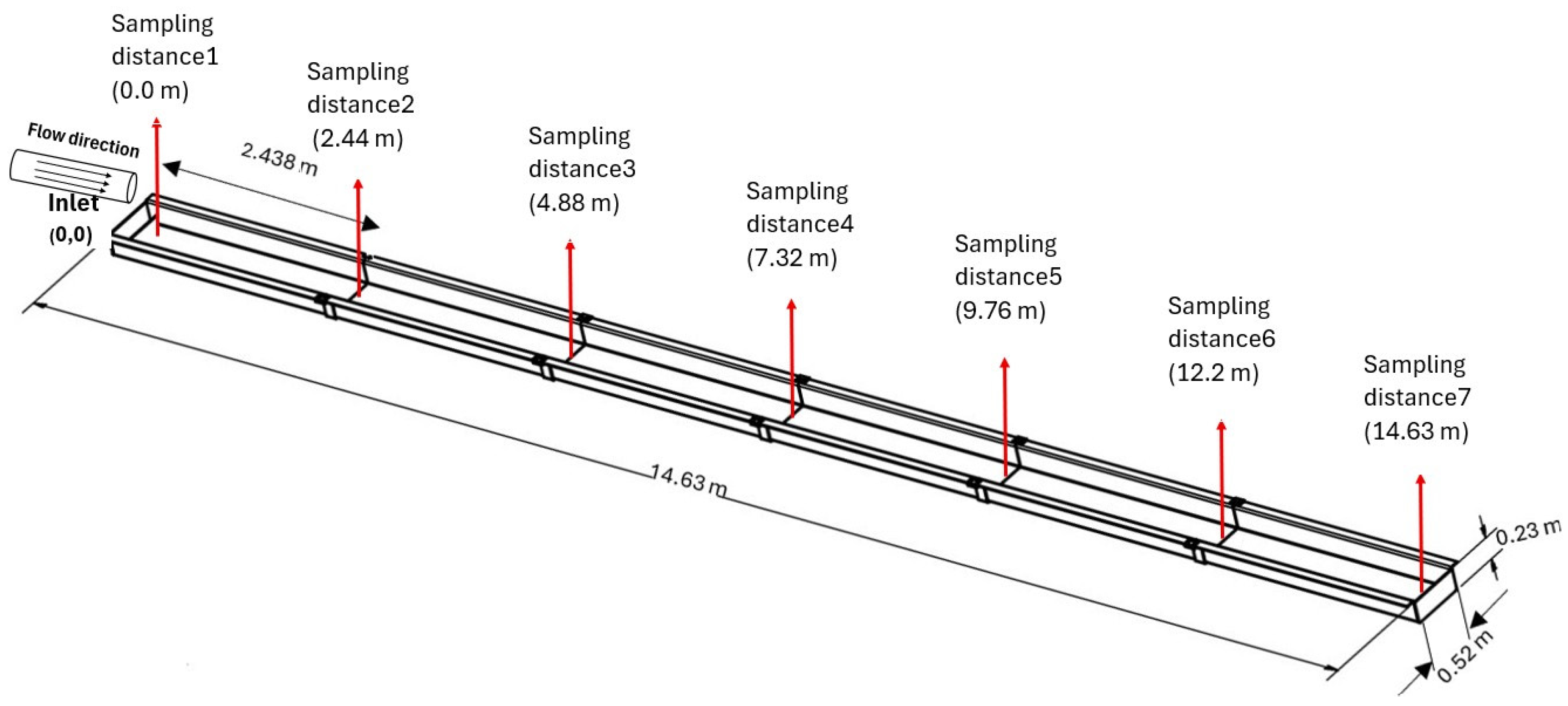
Figure 2.
Flume mounting and experimental procedure of the flume test. a) assembly and alignment of the flume support structure, b) slope adjustment, c) joint sealing, d) tailings homogenization, e) flume test conducting, f) tailings sampling along the flume, and g) flume cleaning.
Figure 2.
Flume mounting and experimental procedure of the flume test. a) assembly and alignment of the flume support structure, b) slope adjustment, c) joint sealing, d) tailings homogenization, e) flume test conducting, f) tailings sampling along the flume, and g) flume cleaning.
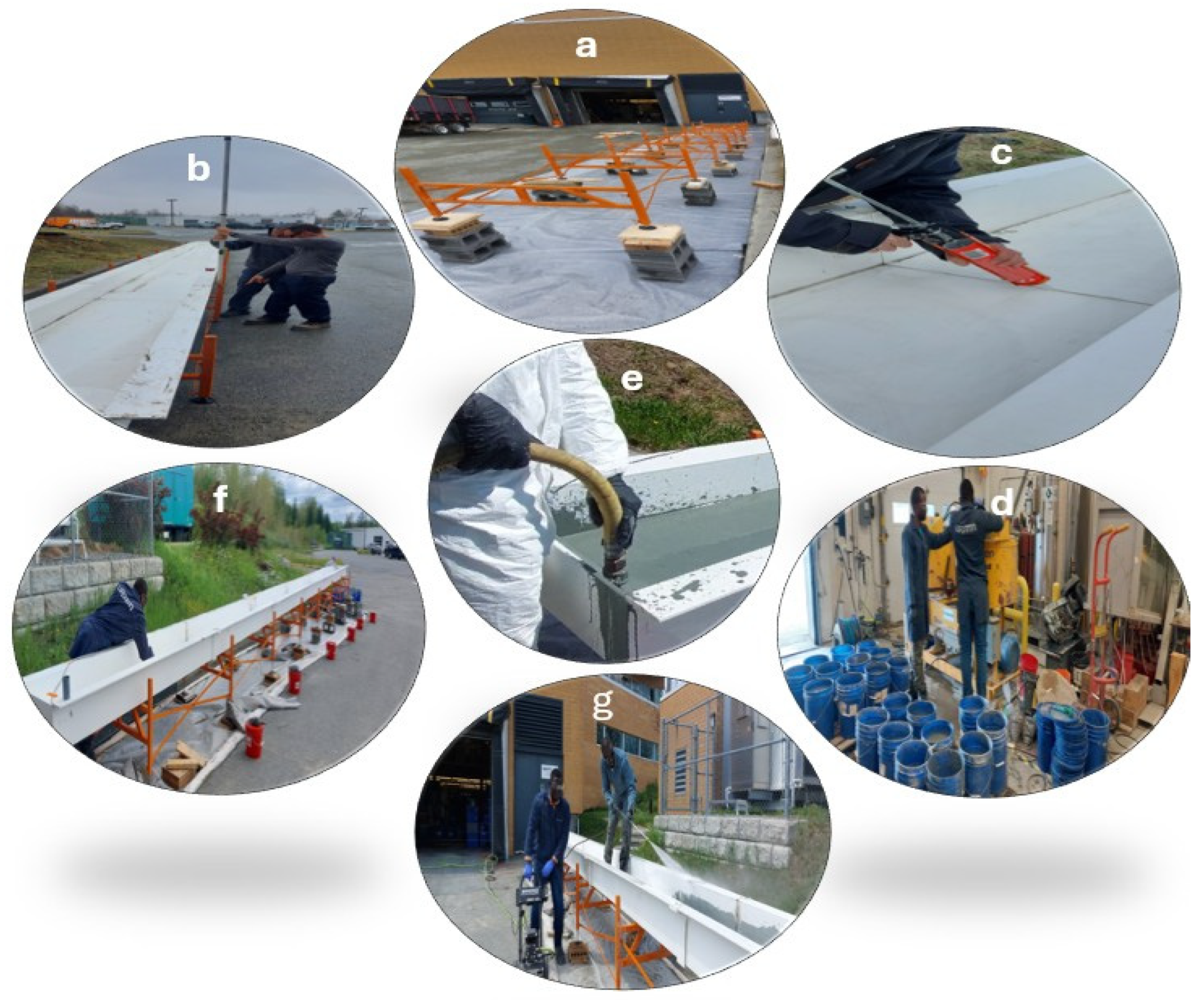
Figure 3.
Photo of the laboratory flume test running.
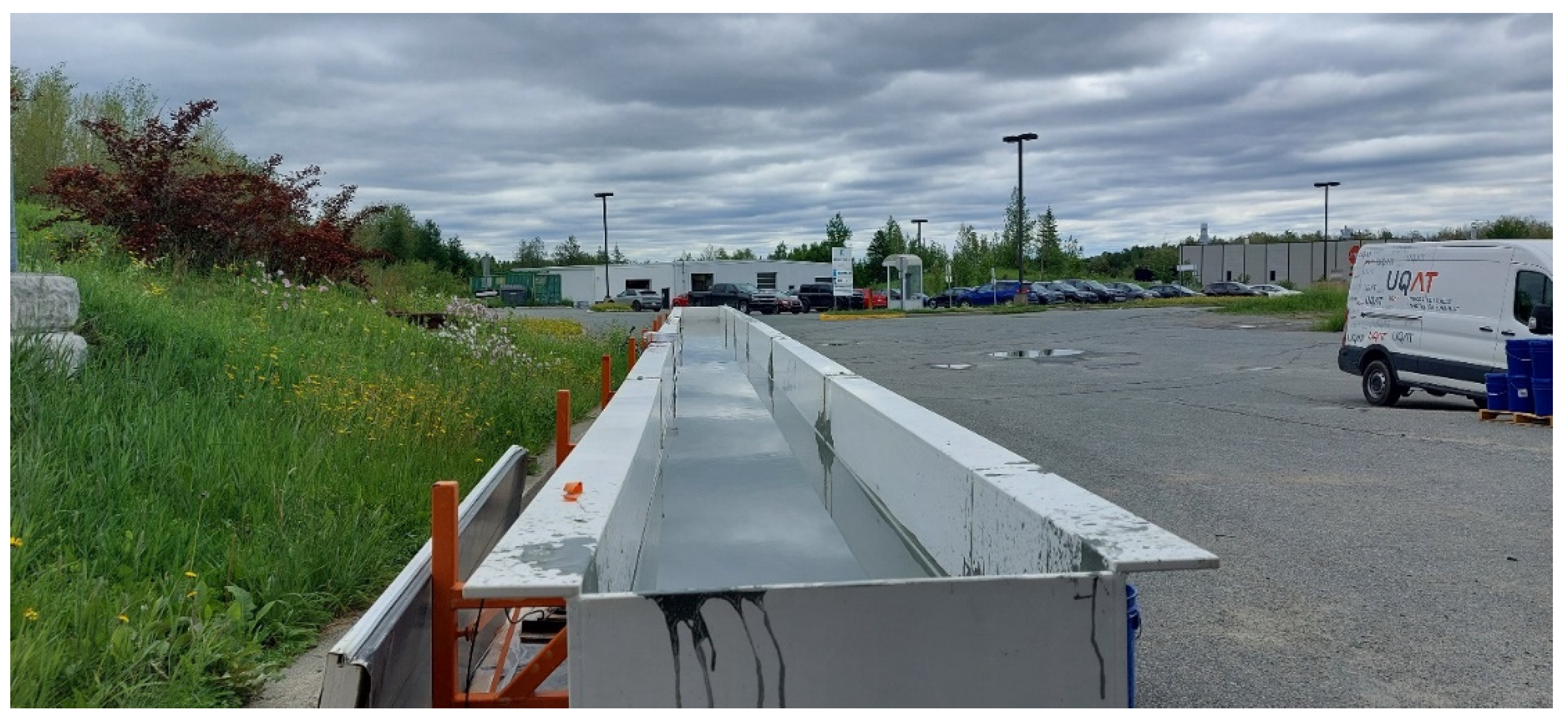
Figure 4.
Testing equipment for rheological analyses: a) AR2000 rheometer, b) vane geometry, and c) post-analysis emptying the stator.
Figure 4.
Testing equipment for rheological analyses: a) AR2000 rheometer, b) vane geometry, and c) post-analysis emptying the stator.
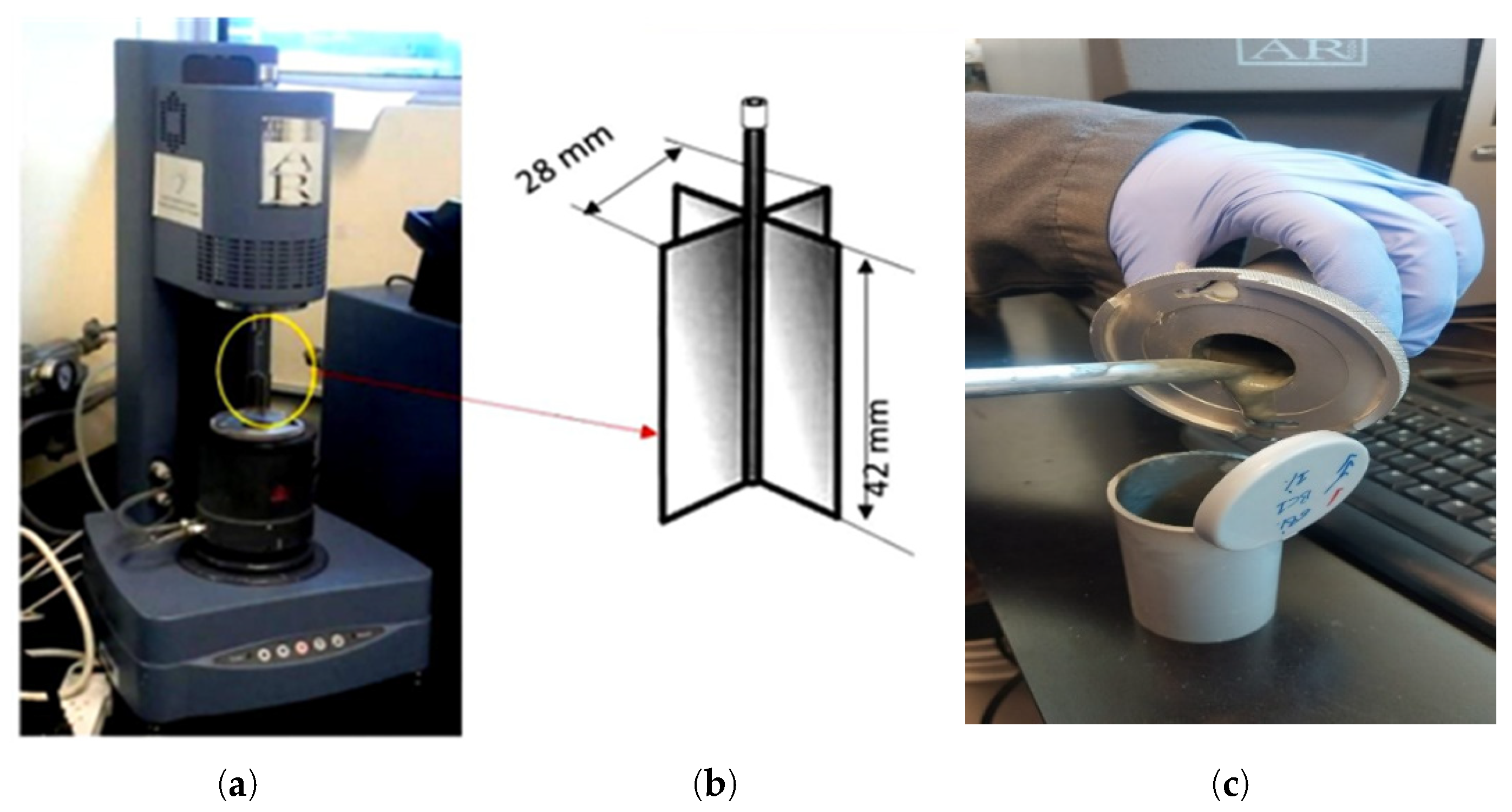
Figure 5.
Typical particle size distribution curves with respect to the sampling distance L along the flume with a slope of 1% for (a) Cw-ini = 69%, (b) Cw-ini = 66%, and (c) Cw-ini = 63%.
Figure 5.
Typical particle size distribution curves with respect to the sampling distance L along the flume with a slope of 1% for (a) Cw-ini = 69%, (b) Cw-ini = 66%, and (c) Cw-ini = 63%.
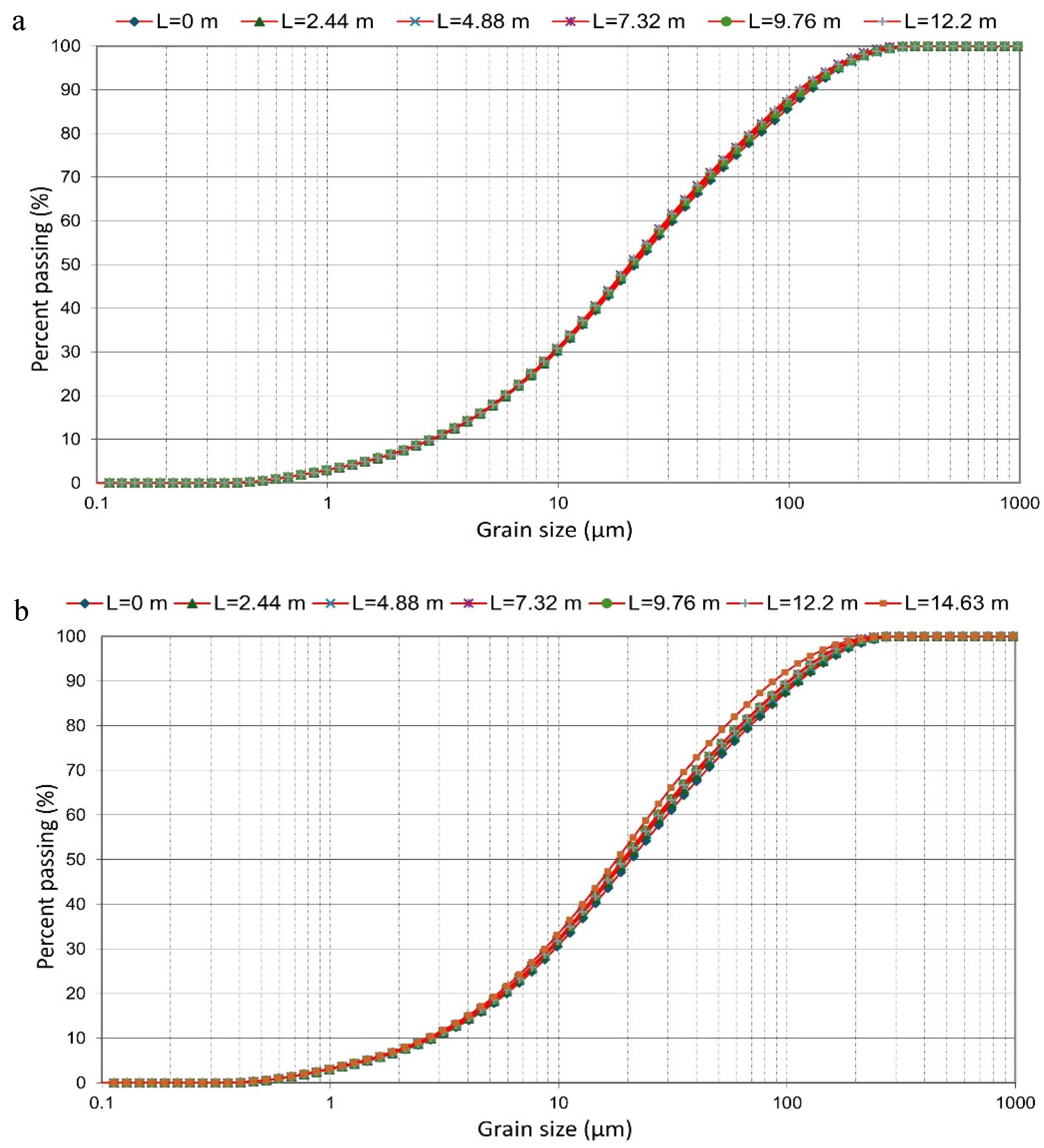
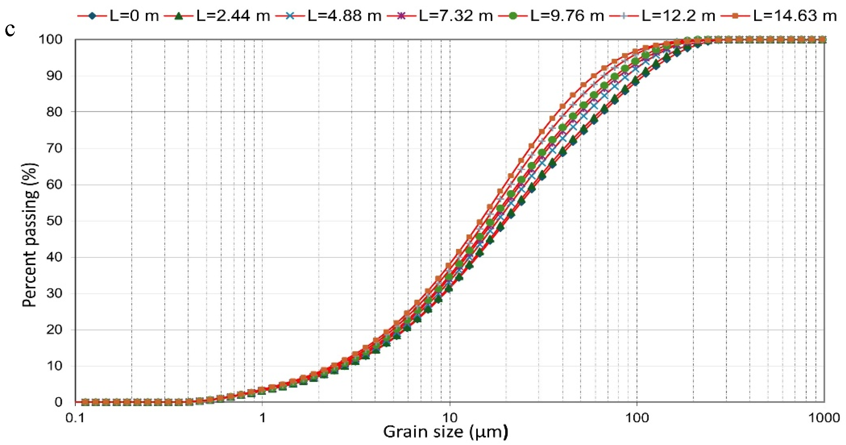
Figure 6.
Variation with the flow distance L along the flume of the mean diameter a) D50 corresponding to 50% passing b) fraction passing 80 µm (P80µm) for slope 1%.
Figure 6.
Variation with the flow distance L along the flume of the mean diameter a) D50 corresponding to 50% passing b) fraction passing 80 µm (P80µm) for slope 1%.
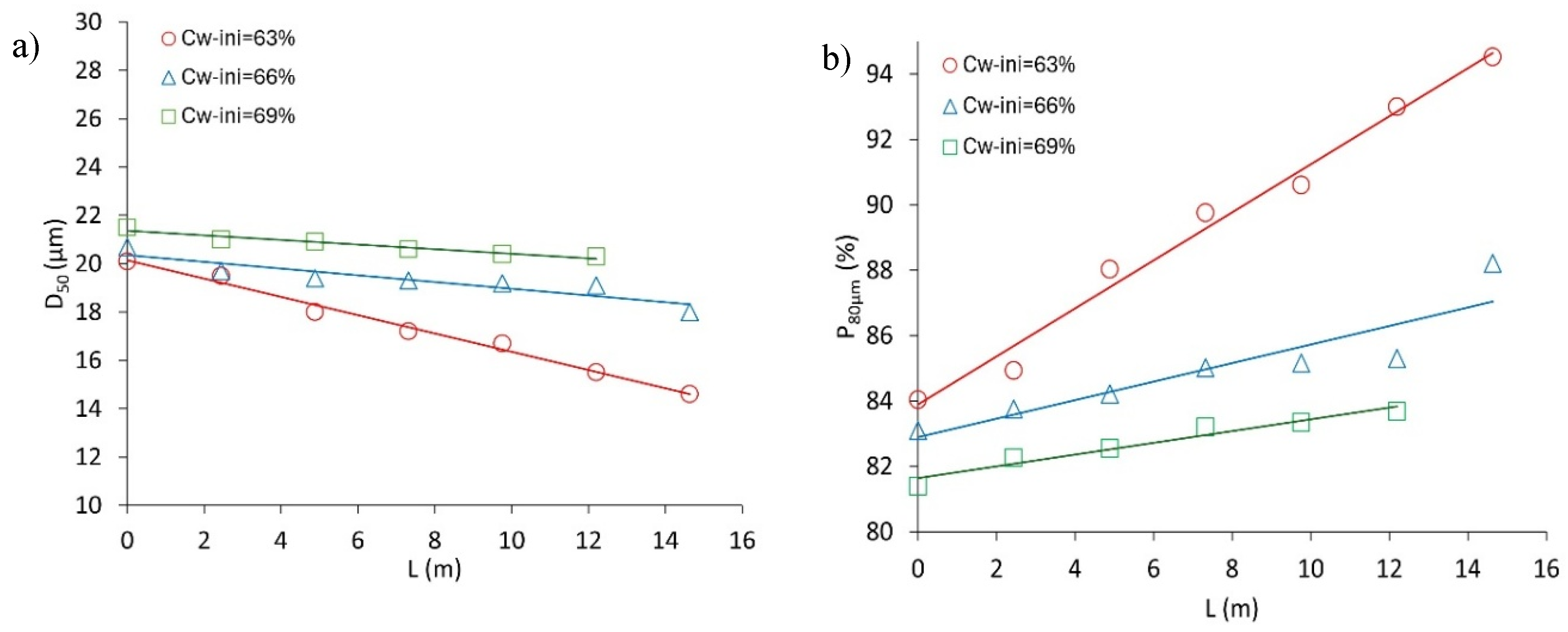
Figure 7.
Variation of solids content (CW) and bulk density (ρ) with respect to the sampling distance L along the flume (marks) together with the fitted linear trend curves (lines) for slopes of 0.5% (a, b) and of 1% (c, d).
Figure 7.
Variation of solids content (CW) and bulk density (ρ) with respect to the sampling distance L along the flume (marks) together with the fitted linear trend curves (lines) for slopes of 0.5% (a, b) and of 1% (c, d).
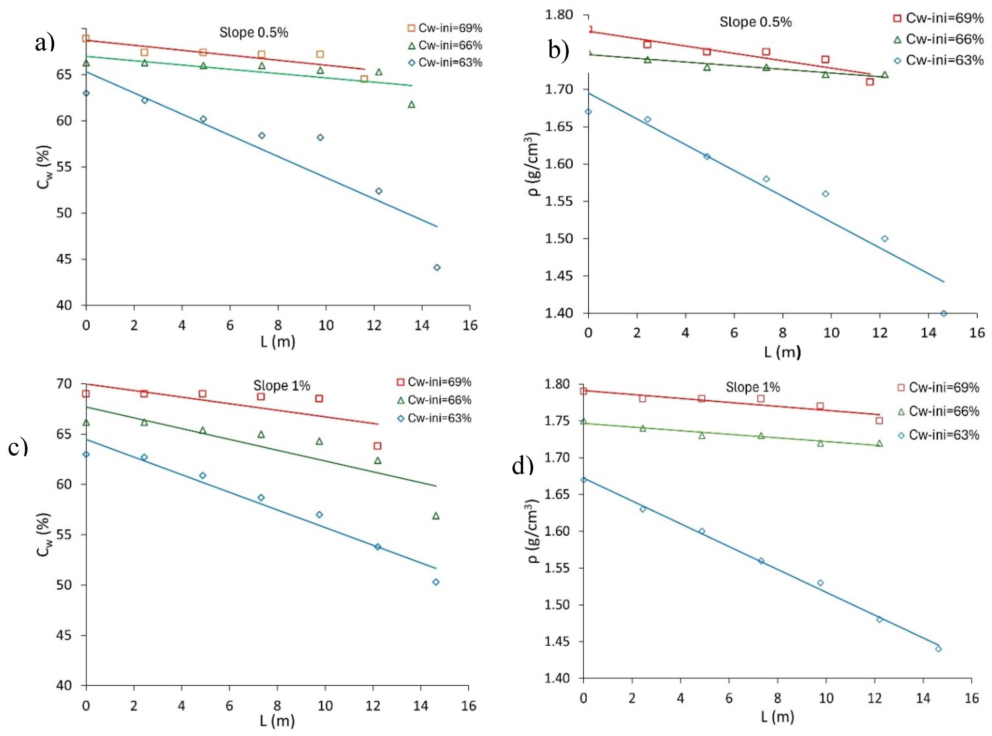
Figure 8.
Typical flow curves (a) and viscosity curves (b) of samples collected along the flume for Cw-ini = 63% and a slope of 0,5% (marks) together with fitting rheological models (lines).
Figure 8.
Typical flow curves (a) and viscosity curves (b) of samples collected along the flume for Cw-ini = 63% and a slope of 0,5% (marks) together with fitting rheological models (lines).
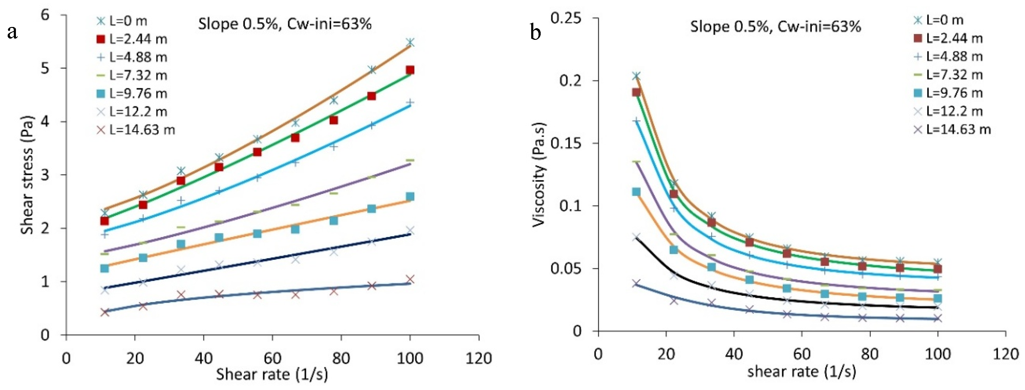
Figure 9.
Boxplots of the variation along the flow distance for the flume at a slope of 0,5% of: (a) shear yield stress τ0-HB (b) viscosity η∞.
Figure 9.
Boxplots of the variation along the flow distance for the flume at a slope of 0,5% of: (a) shear yield stress τ0-HB (b) viscosity η∞.
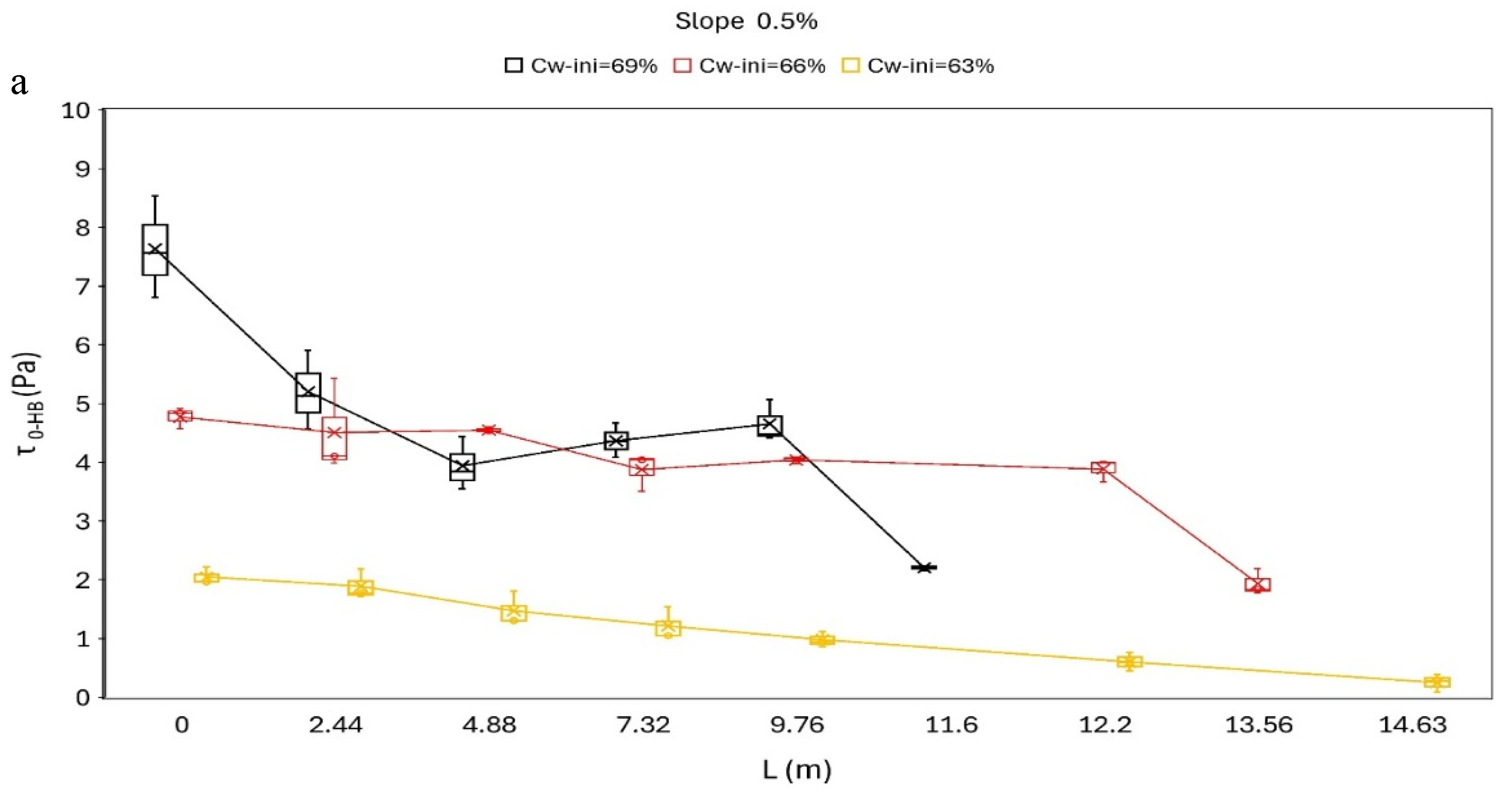
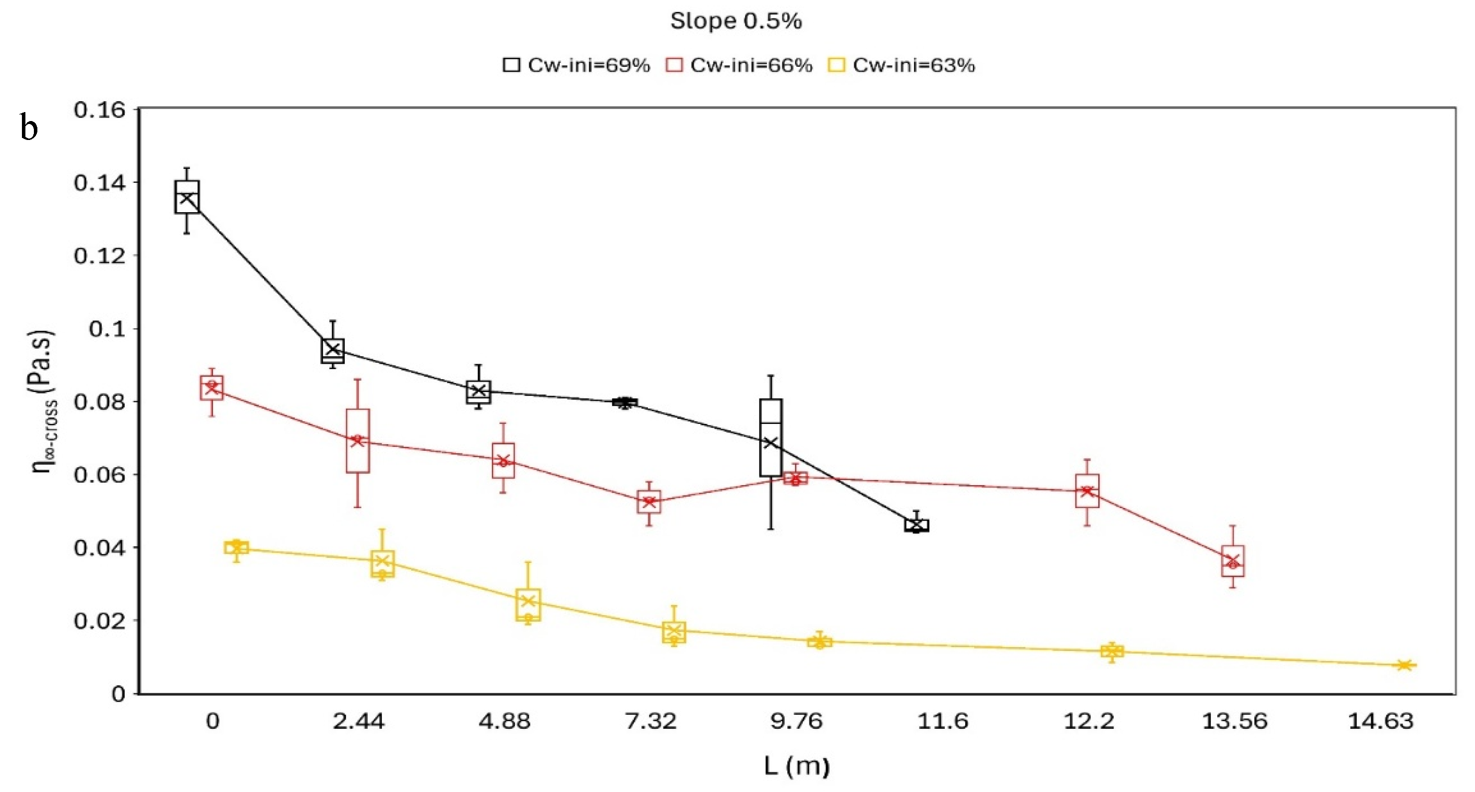
Figure 10.
Boxplots of the variation along the flow distance for the flume at a slope of 1% of: (a) shear yield stress τ0-HB, (b) viscosity η∞.
Figure 10.
Boxplots of the variation along the flow distance for the flume at a slope of 1% of: (a) shear yield stress τ0-HB, (b) viscosity η∞.
Figure 11.
Correlation between SI and initial physiacal and rheological proprties (marks) together with the fitted exponential trend curves (lines): (a) Cw-ini (%), (b) ρini (g/cm3), (c)
(d) (Pa.s).
Figure 11.
Correlation between SI and initial physiacal and rheological proprties (marks) together with the fitted exponential trend curves (lines): (a) Cw-ini (%), (b) ρini (g/cm3), (c)
(d) (Pa.s).
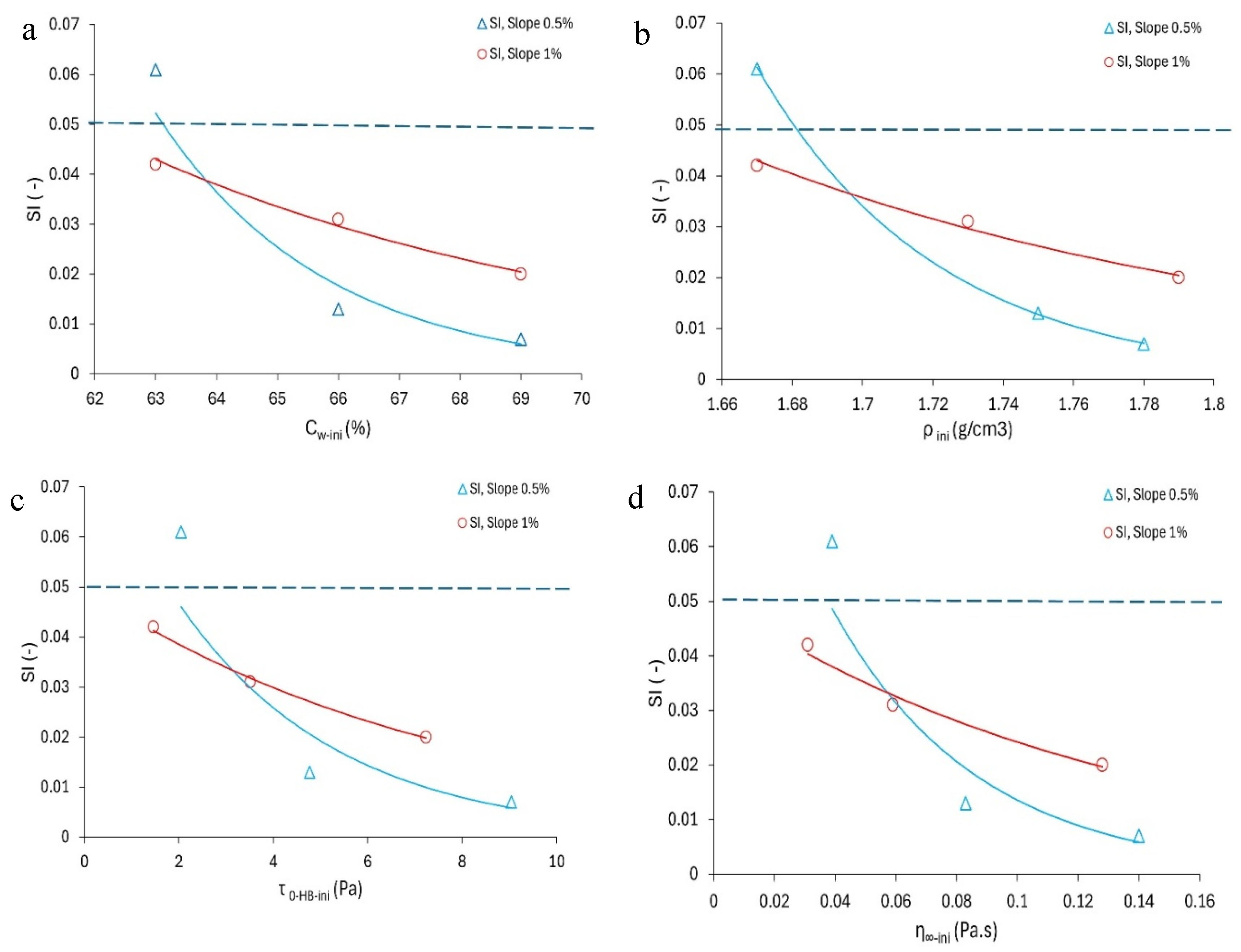
Figure 12.
SI (experimental) vs SI (model prediction).
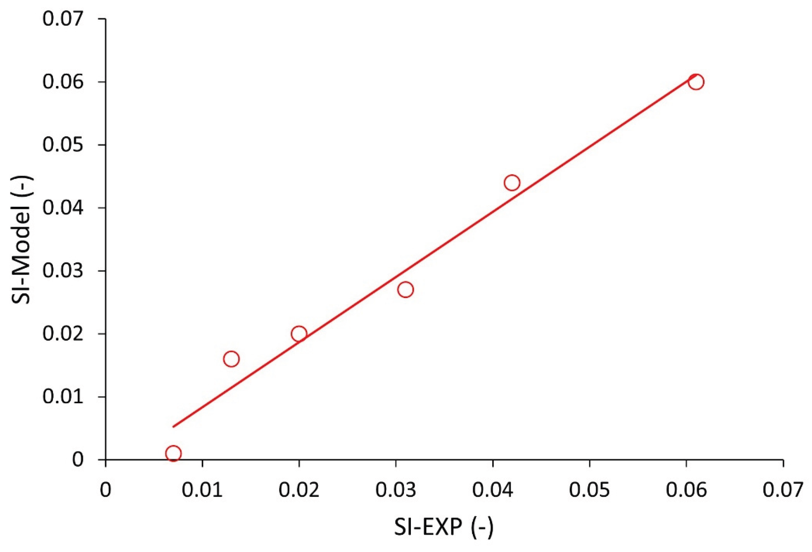
Table 1.
Experimental program.
| Test # | Slope (%) | Cw-ini (%) | Mass of tailings prepared (kg) | Measured density (g/cm3) |
|---|---|---|---|---|
| 1 | 0.5 | 63 | 712 | 1.67 |
| 2 | 66 | 731 | 1.75 | |
| 3 | 69 | 740 | 1.78 | |
| 4 | 1.0 | 63 | 649 | 1.67 |
| 5 | 66 | 711 | 1.73 | |
| 6 | 69 | 695 | 1.79 |
Table 2.
Variables used in the SI model and their units.
| Parameter | Symbol | Unit | Dimensions |
|---|---|---|---|
| Flow running length | |||
| Shear yield stress | |||
| Infinite dynamic viscosity | η∞ | ||
| Flow index | - | - | |
| Slope of flume | - | - | |
| Bulk density | |||
| Segregation Index | - | - |
Table 3.
π-groups by combining the repeating variables with the remaining variables.
| Π groups | Formula |
|---|---|
| Π₁: Shear yield stress () | |
| Π2: Flow index () | |
| Π3: Slope of flume () | |
| Π4: Segregation index () |
Table 4.
Comparison between experimental (Exp.) and predicted (Pred.) SI values.
| Flume Test # | Cw-ini (%) |
(-) | ρini (kg/m3) |
τ HB-ini (Pa) | η∞-ini (Pa.s) |
nini (-) |
Exp. SI (-) | Pred. SI (-) |
|---|---|---|---|---|---|---|---|---|
| 1 | 69 | 0.005 | 1780 | 9.04 | 0.14 | 1.67 | 0.007 | 0.001 |
| 2 | 66 | 0.005 | 1750 | 4.78 | 0.08 | 1.31 | 0.013 | 0.016 |
| 3 | 63 | 0.005 | 1670 | 2.05 | 0.04 | 1.18 | 0.061 | 0.060 |
| 4 | 69 | 0.01 | 1790 | 7.23 | 0.12 | 1.18 | 0.020 | 0.021 |
| 5 | 66 | 0.01 | 1730 | 3.51 | 0.059 | 1.23 | 0.031 | 0.027 |
| 6 | 63 | 0.01 | 1670 | 1.46 | 0.03 | 1.2 | 0.042 | 0.044 |
Disclaimer/Publisher’s Note: The statements, opinions and data contained in all publications are solely those of the individual author(s) and contributor(s) and not of MDPI and/or the editor(s). MDPI and/or the editor(s) disclaim responsibility for any injury to people or property resulting from any ideas, methods, instructions or products referred to in the content. |
© 2026 by the authors. Licensee MDPI, Basel, Switzerland. This article is an open access article distributed under the terms and conditions of the Creative Commons Attribution (CC BY) license (http://creativecommons.org/licenses/by/4.0/).
Copyright: This open access article is published under a Creative Commons CC BY 4.0 license, which permit the free download, distribution, and reuse, provided that the author and preprint are cited in any reuse.


