S-NODE-ANF-RRC: Stochastic Neural ODE for Financial Regime Forecasting and False Alarm Control on JSE Equities

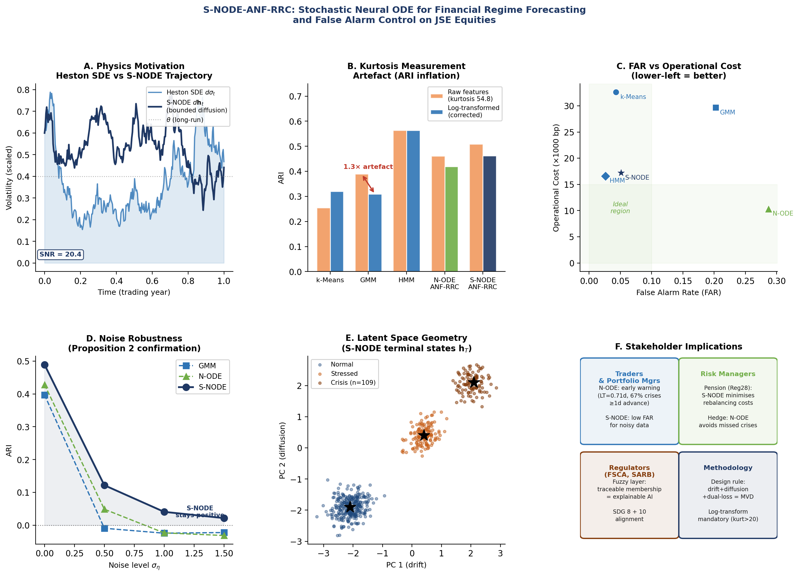
Emerging-market equity exchanges require regime forecasting systems that are continuous in time, robust to heavy-tailed distributions, and optimised against false alarms. No existing method addresses all three simultaneously, and no prior study has reported a crisis false alarm rate on JSE equities. We propose S-NODE-ANF-RRC: a Stochastic Neural ODE embedded within an Adaptive Neuro-Fuzzy Risk-Regime Clustering architecture, motivated by the Heston stochastic volatility framework and integrated by a Milstein scheme with Lyapunov-regularised dual-loss training. The system is evaluated as a one-step-ahead probabilistic forecaster (h = 1 trading day) on 2696 daily observations across 17 JSE securities (March 2015–March 2026). Gaussian mixture clustering on raw features (kurtosis 54.8) inflates ARI by 1.3×; log-transformation corrects this systematic artefact. Two operational profiles emerge after correction: the N-ODE-ANF-RRC achieves the lowest cost (10,350 bp, 65.1% below GMM), longest lead time (0.71 days), and best MCC (0.596); the S-NODE-ANF-RRC achieves the lowest false alarm rate among probabilistic architectures (FAR = 0.051, log-loss = 1.07), with a 42.0% cost reduction versus GMM (bootstrap 95% CI [5, 250, 19, 600] bp; McNemar p = 0.027). Ablation confirms drift, diffusion, and dual-loss as the minimum viable daily-frequency configuration. The interdisciplinary fusion of physics-informed SDE dynamics, time series forecasting, and fuzzy interpretability yields two complementary JSE risk tools: an early-warning forecaster (N-ODE) and a low-false-alarm crisis classifier (S-NODE). Code and data: https://doi.org/10.5281/zenodo.19787658.