Preprint
Article

This version is not peer-reviewed.

Binary Sequences with Low Aperiodic Autocorrelations: Small Peak Sidelobe Levels

Submitted:

12 May 2026

Posted:

13 May 2026

You are already at the latest version

Abstract
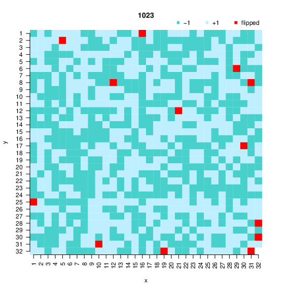
Binary sequences (binary codes), where the elements are −1 or +1, are useful in many fields, including communications, radar, sonar, mathematics, physics, and cryptography. This paper considers binary sequences with low aperiodic autocorrelations and focuses on the small peak sidelobe levels alongside the merit factor. Two families of binary sequences are considered, namely Rudin-Shapiro and Legendre sequences. For both families, we applied a heuristic algorithm to minimize the peak sidelobe levels for sequences of lengths up to 2^16 and 220−1, respectively. The main contribution of the article is two conjectures associated with Legendre sequences: (1) The obtained binary sequences with the best-known peak sidelobe levels have merit factor ≈5.0, (2) The number of elements that differ between the resulting binary sequences and the initial Legendre sequences follows a linear dependence on the sequence length (n), namely ≈0.01n. The Rudin-Shapiro sequences do not exhibit these properties, as worse peak sidelobe level and merit factor values were obtained. The number of elements that differ between the resulting binary sequences and the initial Rudin-Shapiro sequences is also much higher compared to that of the Legendre sequences.
Keywords: 
;  ;  ;  ;  ;  

1. Introduction

A binary sequence of length n is an n-tuple A = ( a 0 , a 1 , , a n 1 ) , where each a i , for i { 0 , 1 , , n 1 } takes the value 1 or + 1 . The aperiodic autocorrelation function of the binary sequence A at shift k is defined as
C A ( k ) : = i = 0 n k 1 a i a i + k for k = 0 , 1 , , n 1 .
The second type of autocorrelation function is periodic. The periodic autocorrelations are usually much easier to study than their aperiodic counterparts [1]. In this work, we consider aperiodic autocorrelations.
Several authors have studied different measures for the collective smallness of the aperiodic autocorrelations of sequences. Two measures of ”smallness” have been used:
1.
merit factor, and
2.
peak sidelobe level.
The merit factor was introduced by Golay [2,3], and it is defined as
F ( A ) : = n 2 2 k = 1 n 1 ( C A ( k ) ) 2 for n > 1 .
The Peak Sidelobe Level (PSL) is defined as
PSL ( A ) : = max 1 k < n | C A ( k ) | .
The autocorrelation function of A at shift 0, C A ( 0 ) , is called the main-lobe level, and it is not included in (3). The rest, C A ( k ) , k = 1 , 2 , , n 1 , are called side-lobe levels. The aperiodic autocorrelation function in (1) is even, since C A ( k ) = C A ( k ) . Therefore, it is sufficient to consider only the shifts k = 0 , 1 , , ( n 1 ) .
Sequence design methods in the literature can be broadly classified into two categories: algebraic constructions and algorithmic design approaches [4]. This work focuses mainly on algorithmic approaches.
In practice, we prefer binary sequences that have a lower PSL value and a higher F value. Some algorithms minimize a combination of metrics to create binary sequences with low aperiodic autocorrelation. A sequence with the optimal PSL usually has a merit factor which is much lower than the optimal merit factor, and vice versa [5,6]. Various algorithms have been proposed recently to solve this challenging optimization problem for F metric. For example, massively parallelized implementation of the memetic tabu search algorithm [7], the quantum approximate optimization algorithm [8], quantum-enhanced memetic tabu search [9], and a competitive NISQ and qubit-efficient solver for the LABS problem. The reader interested in the F metric is referred to the survey [1](Chapter 3.5) and recent works [10,11].
Let A n denote the set of all binary sequences of length n. We would like to understand the behavior of
μ ( n ) : = min A A n PSL ( A ) ,
as n . If someone wishes to compute μ ( n ) for a given length n, then they need, using the most naive approach, to probe 2 n different binary sequences. The exponential term of the time complexity can be reduced from O ( 2 n ) to approximately O ( 1 . 4 n ) by more efficient algorithms [12,13]. The considerable numerical computation effort in finding binary sequences with small PSL values has been put in by various authors, and, nowadays, μ ( n ) for n 61 and n = 64 are known, while for larger lengths, the best-known PSL values are reported in the literature. For 71 n 105 , the PSL values are presented in [14]. Currently, results for all lengths 106 n 300 are reported in [5,15,16], PSL values for selected lengths for 301 n 4000 are published by several authors (see [17] and references therein), for some n up to 8191 in [18,19], and for even longer n (up to 10 6 ) in [5,17,20,21,22] and up to 2 25 1 in [13].

1.1. Contributions of the Paper

In this paper, two families of binary sequences are considered, namely Rudin-Shapiro and Legendre sequences. Experimental works include the minimization of the peak sidelobe levels of Legendre sequences of length up to 2 20 1 .
Based on numerical experimentation, two conjectures associated with Legendre sequences are proposed:
  • The obtained resulting binary sequences with the best-known peak sidelobe levels have merit factor 5.0 . It appears to be close to a whole number.
  • The number of elements that differ between the resulting binary sequences and the initial Legendre sequences follows a linear dependence on the sequence length (n), namely 0.01 n .
Additional experimentation indicates that no such results can be observed with the Rudin-Shapiro sequences, where worse peak sidelobe level and merit factor values were obtained.

1.2. Structure of the Paper

The paper is organized as follows. Section 2 provides the necessary background knowledge to understand the main ideas of the paper. Related work is discussed in Section 3. Section 4 outlines the methodology used for the experimental part. Extensive experiments conducted to find binary sequences with small peak sidelobe levels and experimental results are presented in Section 5. Based on the results obtained, we also proposed two conjectures in this section. Section 6 highlights some additional notes. Finally, Section 7 summarizes the findings and concludes the paper.

2. Preliminary

In this section, we give a brief overview of some families of binary sequences, how we generate them, their properties, and some known results.
The Rudin-Shapiro sequence requires a four-letter alphabet with the following substitution rule [23]:
( 1 ) S ST , T SU , U VT , V VU , ( 2 ) S , T 0 , U , V 1 .
The first symbolic generations are:
w ( 0 ) = S , w ( 1 ) = ST , w ( 2 ) = STSU , w ( 3 ) = STSUSTVT ,
Applying the binary conversion rules to the Rudin-Shapiro symbolic generations yields:
w ( 0 ) = 0 , w ( 1 ) = 00 , w ( 2 ) = 0001 , w ( 3 ) = 00010010 ,
Changing each symbol 0 to 1 yields the binary sequence in our format. The length of the Rudin-Shapiro sequence is n = 2 m , where m { 1 , 2 , } .
Calculations by Littlewood show that the Rudin–Shapiro sequences have low mean square autocorrelation [24]. We now examine the lower and upper bounds for PSL values of Rudin–Shapiro sequences. Here we use the abbreviated text from [24] [Theorem 3, p. 3457].
Theorem 1 
(Katz and van der Linden [24]). If n is a nonnegative integer and x n and y n the n-th Rudin-Shapiro sequence and its companion, then PSL ( x n ) = PSL ( y n ) , and we have the lower and upper bound
0.382159 . . . lim sup n PSL ( x n ) α 0 n 0.660113 . . .
where α 0 = 1.658967 . . . is the real root of X 3 + X 2 2 X 4 .
The difference between binary sequences A and B, both of length n, can be written as the Hamming distance:
d = d ( A , B ) = i = 0 n 1 d i ,
where
d i = 1 , A i B i , 0 , A i = B i .
We are interested in how different the two binary sequences are, where the first sequence is an initial sequence and the second sequence has an optimized value of PSL . The second sequence is obtained during the optimization process using the heuristic algorithm, presented in [17].
Ein-Dor et al. [25] proposed an “educated guess” about the growth rate of the function μ ( n ) .
Conjecture 1 
(Ein-Dor et al. [25]). As n , we have
μ ( n ) n d , where d = 0.435 . . . .
Theorem 2  
(Moon and Moser [26]).
(i) 
For any fixed ϵ > 0 , the proportion of sequences A A n such that μ ( n ) ( 2 + ϵ ) n log n approaches 1 as n .
(ii) 
If K ( n ) is any function of n such that K ( n ) = o ( n ) , then the proportion of sequences A A n for which μ ( n ) approaches 1 as n .
Theorem 2, the only proven PSL result for general binary sequences, examines the growth rate of the peak sidelobe level of almost all binary sequences and this growth rate lies between order n and order n log n .
A Legendre sequence A of length p, where p is an odd prime number, is defined as:
A ( k ) = k p , for 0 k < p ,
where k p is the Legendre symbol [27,28]. The Legendre symbol is defined as:
k p = + 1 , if p | k or k is a quadratic residue modulo p , 1 , otherwise .
Note that we use the convention that k p = 1 if k = 0 .
Dimitrov [21] gave a complete list of all PSL-optimal Legendre sequences, with or without rotations, for lengths up to 432100. The numerical experiments suggest that the PSL values of all PSL-optimal Legendre sequences, with or without rotations, and with lengths n greater than 235723, are strictly greater than n .
Let us consider another family of binary sequences, namely Galois sequences, also called m-sequences. Galois sequences can be efficiently generated using linear feedback shift registers [29]. There is a direct correspondence between m-sequences of degree q and primitive polynomials of degree q over GF(2) [30].
Dmitriev and Jedwab [13] performed experiments on m-sequences up to length 2 25 1 and they showed numerically:
Conjecture 2  
(Dmitriev and Jedwab [13]). The PSL of all m-sequences of length n appears to grow like O ( n · log log n ) .
In the same work, Dmitriev and Jedwab also numerically showed:
Conjecture 3  
(Dmitriev and Jedwab [13]). The PSL of almost all m-sequences of length n appears to grow like Θ ( n ) .
Numerical evidence in Conjecture 3 relies on an algorithm for calculating the maximum PSL over all cyclic shifts of an m-sequence for m 25 . The mean (taken over all primitive elements α of GF(n+1) [13,31]) of the maximum PSL over all cyclic shifts appears to be approximately 1.31 n for all values of m between 13 and 25.

4. Methodology

We will analyze the PSL values of the binary sequences that were optimized a heuristic algorithm. The initial binary sequences, which served as seeds for the optimization algorithm, were selected from two well-known families of binary sequences, namely the Rudin-Shapiro and Legendre sequences. The applied heuristic algorithm [17] minimizes only the PSL value during the optimization process. We will be interested in the difference between the initial and the optimized binary sequence. For the sequence obtained after optimization, we will also calculate the merit factor and compare it with the merit factor of the initial sequence, whose merit factor is known. The obtained results will also be compared with results from the literature.
The length of Rudin-Shapiro sequence is n = 2 m and our heuristic algorithm performed the optimization process on that length. We denote the initial and optimized Rudin-Shapiro sequences as B i n i t R S and B o p t R S , respectively.
A Legendre sequence is defined for length p, where p is an odd prime number. We wish to use a binary sequence of length n = 2 m 1 , so we applied the following procedure to ensure the length. We used the first prime p that satisfies n p . A Legendre binary sequence of length p is generated using (7) and rotated by 1/4. It is then truncated, if needed, to ensure that the length of the initial binary sequence is equal to n. We denote the initial, 1/4-rotated, and truncated Legendre sequence as B i n i t L e g and the optimized Legendre sequence B o p t L e g .

5. Experiments

In this section, we present the results of finding good PSL values for two families of binary sequences, and then give two conjectures.

5.1. Results on Rudin-Shapiro Sequences

The construction of the Rudin–Shapiro sequences is described in Section 2. For selected lengths, the lower (LB) and upper (UB) bounds alongside the PSL value of the Rudin-Shapiro sequences are shown in Table 1. The bounds are calculated using Theorem 1.
Next, we present experimental results of optimized Rudin-Shapiro sequences. For this purpose, we used the heuristic algorithm [17]. The algorithm started with the initial Rudin-Shapiro sequence ( B i n i t R S ) with length n, and during the optimization process, the algorithm made improvements to the binary sequence by changing a small number of elements of the sequence, yielding the optimized Rudin-Shapiro sequence ( B o p t R S ).
Table 2 shows PSL of the optimized sequence ( B o p t R S ), and difference between the initial Rudin-Shapiro sequence ( B i n i t R S ) and the optimized sequence ( B o p t R S ) for 10 m 16 . Comparing the PSL values in Table 1 and Table 2, it can be seen that the PSL values of the initial sequences are much higher than those of the optimized sequences. For example, for m = 16 , the PSL values are 1717 and 209, respectively. Differences between the Rudin-Shapiro sequences (initial) and the optimized sequences are between 30% and 50%. This indicates that the heuristic algorithm had to flip quite a few elements of the binary sequence.
When we compare the corresponding merit factors, we notice that the merit factors in the optimized sequences increased from the initial F = 3.0 , which is known for Rudin-Shapiro sequences, to values between 3.8 and 4.2 . In general, we can see that with the improvement of the PSL value (lower value is better), the merit factor value also managed to improve (higher value is better).

5.2. Results on Legendre Sequences

Table 3 shows PSL and merit factor values of the optimized sequence starting from the initial Legendre sequence for lengths n = 2 m 1 , m { 10 , 20 } . Values PSL / n show an increasing trend, but all of them are lower than 0.75 . Merit factor values are very close to 5.0 , except for the two shortest lengths (1023 and 2047), where F is 4.8 . Note that our heuristic algorithm applied the minimization criteria on the PSL. The difference (d) between the initial Legendre sequence ( B i n i t L e g ) and the optimized sequence ( B o p t L e g ), and the ratio d / n in percent are presented in the last two columns. One can see that the ratio d / n follows a constant value that is close to 1% for m { 12 , 13 , , 20 } .
Comparing the optimized PSL values of Rudin-Shapiro (Table 2) and the optimized Legendre (Table 3) sequences, we can see that the PSL values of optimized Rudin-Shapiro sequences are much higher. Also, the differences between the initial and optimized binary sequences are much higher for Rudin-Shapiro compared to Legendre ones, i.e., more than 30% for Rudin-Shapiro and only approximately 1% for Legendre.
Results in Table 3 are taken from work [17], except for m = 13 , 18 , 19 , and 20, which were obtained using the heuristic algorithm also presented in [17]. PSL values for m = 18 , 19 , and 20 were improved by 1, 1, and 4, respectively, and are currently the best-known values. Note, the best-known PSL is 65 for m = 13 [17].
Let us briefly compare PSL results of optimized Legendre sequences with selected results from the literature. Mow et al. [32] reported PSL = 61 and F = 3.4589 for n = 4096 , while Zhang et al. [37] obtained PSL = 56 and F = 4.8197 . Dimitrov et al. [15] gave PSL = 77 for n = 8191 . PSL = 71 and F = 4.00397 for n = 8191 , and PSL = 50 and F = 4.0049 for n = 4095 are reported by Bošković and Brest [34]. Brest and Bošković [5] gave PSL = 70 and PSL = 48 for n = 8191 and 4095, respectively. In all five works just mentioned, the algorithms were run from a random binary sequence, and from the comparison of their results, we can see slightly higher PSLs (i.e., worse) than those shown in Table 3. Also, the merit factors are usually lower than 5.0.
Figure 1, Figure 2, and Figure 3 illustrate the differences between the initial Legendre sequence ( B i n i t L e g ) and the resulting optimized sequence ( B o p t L e g ) for length 1023, 2047, and 4095, respectively. Each binary sequence is represented as a square, the sequence starts in the first row in the upper left corner, followed by the second row, etc., the sequence ends in the last row in the lower-right corner. The elements that represent the difference between the initial and resulting sequences are marked in red. For example, there are 40 flipped components, i.e., differences, between the compared sequences (marked with red color) in Figure 3, which is 40 / 4095 = 0.009768 1 % .
Figure 4 shows how the difference d and merit factor F changed versus the number of PSL value improvements during the optimization process on the sequence of length 131071 ( 2 17 1 ). The merit factor initially starts at 6.0 , then decreases to values below 4.4 , followed by a more pronounced increase, eventually approaching approximately 5.0 toward the end. One can also observe the increasing and decreasing trends in the number of flipped elements d from the initial sequence. At the end, d = 1394 and d / n = 0.0106 1 % .
Figure 5 shows the values of PSL / n log n , PSL / n log log n , and PSL / n , respectively. The values of PSL / n log n and PSL / n log log n show a non-increasing trend for m 10 , while PSL / n shows an increasing trend for m 10 . This suggests, based on experimental investigation up to 2 20 1 , that currently best-known PSL appears to grow like O ( n log log n ) .

5.3. Two Conjectures

Based on the experimental results in this section, we provide the following two conjectures.
Conjecture 4.  
Let B o p t L e g be an optimized Legendre sequence, then F ( B o p t L e g ) 5.0 .
Conjecture 5.  
d ( B i n i t L e g , B o p t L e g ) 0.01 n .
Conjecture 4 is conjectured based on the results of optimized binary sequences ( B o p t L e g ) of length 2 20 1 , where the merit factors are approximately 5.0.
The asymptotic merit factor of the Legendre sequence B i n i t L e g appears to be close to a whole number, although we do not yet have a good explanation as to why. Based on experimental results, a similar observation can be seen for the merit factor of the optimized Legendre sequence B o p t L e g , i.e., it is also close to a whole number. Note that the difference between the two merit factors is 1.
Conjecture 5 shows that
d ( B i n i t L e g , B o p t L e g ) n 0.01 ,
i.e., ratio d / n appears to be close to a constant value 0.01 .

6. Discussion

In the discussion, we highlight three notes:
1.
An optimization algorithm can take into account Conjecture 5 as heuristic knowledge. Let (integer) value q = 0.01 n . Then the number of possible choices of q elements within a binary sequence of length n is equal to n q . Suppose n = 1023 , then the number of possible choices is approximately 3.3 × 10 23 . It becomes a huge value when n is increased.
2.
Since the search space for finding (optimal) binary sequences is huge, the obtained PSLs in Table 3 are not necessarily optimal. Binary sequences with even better PSLs may be found in the future, but this will likely require considerable computational effort.
3.
Conjectures 2 and 3 proposed by Dmitriev and Jedwab [13] show the excellent grow rate of m-sequences. These sequences may also be good candidates to be used as seed/initial sequences in our heuristic algorithm. This can be a great challenge for further work.

7. Conclusions

In this paper, the experimental work includes the minimization of the peak sidelobe of binary sequences. Two families of binary sequences were considered, namely Rudin-Shapiro and Legendre sequences. The main contributions are as follows: Based on numerical experimentation with Legendre sequences of length up to 2 20 1 two conjectures associated with Legendre sequences are proposed: (1) The obtained resulting binary sequences with the best-known peak sidelobe levels have merit factor 5.0 , and (2) The number of elements that differ between the resulting binary sequences and the initial Legendre sequences follows a linear dependence on the sequence length (n), namely 0.01 n . Three new best-known PSL values were obtained for binary sequences of lengths n = 2 m 1 for m = 18 , 19 , and 20.

Author Contributions

Conceptualization, J.B. and B.B.; methodology, J.B., B.P. and B.B.; software, J.B., A.B.; validation, J.B., J.P. and B.P.; investigation, J.B. and B.B.; writing—original draft preparation, J.B.; writing—review and editing, J.B., B.P., J.P., A.B. and B.B.; visualization, J.B., B.P., J.P. and A.B. All authors have read and agreed to the published version of the manuscript.

Funding

This work was supported by the Slovenian Research and Innovation Agency (research core funding P2-0041 — Computer Systems, Methodologies, and Intelligent Services).

Data Availability Statement

The data is available at https://github.com/J-Brest/LABS.

Acknowledgments

The authors would like to acknowledge the Slovenian Initiative for National Grid (SLING) for using computational resources for performing some experiments in this paper.

Conflicts of Interest

The authors declare no conflicts of interest.

References

  1. Schmidt, K.U. Sequences with small correlation. Des. Codes Cryptogr. 2016, 78, 237–267. [Google Scholar] [CrossRef]
  2. Golay, M. A class of finite binary sequences with alternate auto-correlation values equal to zero (corresp.). IEEE Trans. Inf. Theory 1972, 18, 449–450. [Google Scholar] [CrossRef]
  3. Golay, M. The merit factor of Legendre sequences (corresp.). IEEE Trans. Inf. Theory 1983, 29, 934–936. [Google Scholar] [CrossRef]
  4. Zhang, M.; Adhikary, A.R.; Yang, Y.; Zhou, Z.; Fan, P. Designing Unimodular Arrays With Low Correlation Sidelobes for Omnidirectional Transmission in Massive MIMO Systems. IEEE Trans. Commun. 2026, 74, 5670–5683. [Google Scholar] [CrossRef]
  5. Brest, J.; Bošković, B. Low Autocorrelation Binary Sequences: Best-Known Peak Sidelobe Level Values. IEEE Access 2021, 9, 67713–67723. [Google Scholar] [CrossRef]
  6. Brest, J.; Brest, A.; Pšeničnik, B.; Popič, J.; Borko, B. Oddaljenost neperiodičnih binarnih zaporedij glede na dve meri avtokorelacijskih lastnosti. Elektrotehniski Vestn. 2025, 92, 97–103. (In Slovene). Available online: https://ev.fe.uni-lj.si/3-2025/Brest.pdf.
  7. Zhang, Z.; Shen, J.; Kumar, N.; Pistoia, M. New Improvements in Solving Large LABS Instances Using Massively Parallelizable Memetic Tabu Search. arXiv 2025, arXiv:2504.00987. [Google Scholar] [CrossRef]
  8. Shaydulin, R.; Li, C.; Chakrabarti, S.; DeCross, M.; Herman, D.; Kumar, N.; Larson, J.; Lykov, D.; Minssen, P.; Sun, Y.; et al. Evidence of scaling advantage for the quantum approximate optimization algorithm on a classically intractable problem. Sci. Adv. 2024, 10, eadm6761. [Google Scholar] [CrossRef]
  9. Cadavid, A.G.; Chandarana, P.; Romero, S.V.; Trautmann, J.; Solano, E.; Patti, T.L.; Hegade, N.N. Scaling advantage with quantum-enhanced memetic tabu search for LABS. arXiv 2025, arXiv:2511.04553. [Google Scholar] [CrossRef]
  10. Chen, Y.; Lin, R. Computationally Efficient Long Binary Sequence Designs with Low Autocorrelation Sidelobes. IEEE Trans. Aerosp. Electron. Syst. 2022, 58, 1966–1980. [Google Scholar] [CrossRef]
  11. Pšeničnik, B.; Mlinarič, R.; Brest, J.; Bošković, B. Dual-step optimization for binary sequences with high merit factors. Digit. Signal Process. 2025, 165, 105316. [Google Scholar] [CrossRef]
  12. Coxson, G.; Russo, J. Efficient exhaustive search for optimal-peak-sidelobe binary codes. IEEE Trans. Aerosp. Electron. Syst. 2005, 41, 302–308. [Google Scholar] [CrossRef]
  13. Dmitriev, D.; Jedwab, J. Bounds on the growth rate of the peak sidelobe level of binary sequences. Adv. Math. Commun. 2007, 1, 461–475. [Google Scholar] [CrossRef]
  14. Nunn, C.J.; Coxson, G.E. Best-known autocorrelation peak sidelobe levels for binary codes of length 71 to 105. IEEE Trans. Aerosp. Electron. Syst. 2008, 44, 392–395. [Google Scholar] [CrossRef]
  15. Dimitrov, M.; Baitcheva, T.; Nikolov, N. On the Generation of Long Binary Sequences With Record-Breaking PSL Values. IEEE Signal Process. Lett. 2020, 27, 1904–1908. [Google Scholar] [CrossRef]
  16. Dimitrov, M.; Baicheva, T.; Nikolov, N. Hybrid Constructions of Binary Sequences With Low Autocorrelation Sideobes. IEEE Access 2021, 9, 112400–112410. [Google Scholar] [CrossRef]
  17. Brest, J.; Popič, J.; Herzog, J.; Bošković, B. An efficient algorithm for designing long aperiodic binary sequences with low auto-correlation sidelobes. IEEE Access 2024, 12, 108921–108927. [Google Scholar] [CrossRef]
  18. Bose, A. Waveform Synthesis for Active Sensing with Emerging Applications. PhD thesis, University of Illinois at Chicago, 2021. [Google Scholar]
  19. Bose, A.; Soltanalian, M. Constructing binary sequences with good correlation properties: An efficient analytical-computational interplay. IEEE Trans. Signal Process. 2018, 66, 2998–3007. [Google Scholar] [CrossRef]
  20. Lin, R.; Soltanalian, M.; Tang, B.; Li, J. Efficient Design of Binary Sequences With Low Autocorrelation Sidelobes. IEEE Trans. Signal Process. 2019, 67, 6397–6410. [Google Scholar] [CrossRef]
  21. Dimitrov, M. On the aperiodic autocorrelations of rotated binary sequences. IEEE Commun. Lett. 2021, 25, 1427–1430. [Google Scholar] [CrossRef]
  22. Lin, R.; Chen, Y.; So, H.C.; Li, J. On Binary Sequence Design via PSL Minimization. IEEE Signal Process. Lett. 2024, 31, 151–155. [Google Scholar] [CrossRef]
  23. Ximenes, J.J.; Pires, M.A.; Villas-Bôas, J.M. Enhanced spreading in continuous-time quantum walks using aperiodic temporal modulation of defects. Phys. Rev. A 2026, 113, 022410. [Google Scholar] [CrossRef]
  24. Katz, D.J.; van der Linden, C.M. Peak Sidelobe Level and Peak Crosscorrelation of Golay–Rudin–Shapiro Sequences. IEEE Trans. Inf. Theory 2022, 68, 3455–3473. [Google Scholar] [CrossRef]
  25. Ein-Dor, L.; Kanter, I.; Kinzel, W. Low autocorrelated multiphase sequences. Phys. Rev. E 2002, 65, 020102. [Google Scholar] [CrossRef]
  26. Moon, J.; Moser, L. On the correlation function of random binary sequences. SIAM J. Appl. Math. 1968, 16, 340–343. [Google Scholar] [CrossRef]
  27. Jedwab, J.; et al. A Survey of the Merit Factor Problem for Binary Sequences. In Proceedings of the SETA; Springer, 2004; pp. 30–55. [Google Scholar] [CrossRef]
  28. Baden, J. Efficient Optimization of the Merit Factor of Long Binary Sequences. IEEE Trans. Inf. Theory 2011, 57, 8084–8094. [Google Scholar] [CrossRef]
  29. Golomb, S.W. Shift Register Sequences Holden-Day; San Francisco, 1967. [Google Scholar]
  30. Golomb, S.W. Periodic binary sequences: solved and unsolved problems. In Proceedings of the Sequences, Subsequences, and Consequences: International Workshop, SSC 2007, Los Angeles, CA, USA, May 31-June 2, 2007; Springer, 2007; pp. 1–8. Available online: https://link.springer.com/chapter/10.1007/978-3-540-77404-4_1.
  31. Jedwab, J. What can be used instead of a Barker sequence? Contemp. Math. 2008, 461, 153–178. Available online: https://www.sfu.ca/~jed/Papers/Jedwab.%20Barker%20Sequence%20Alternatives.%202008.pdf.
  32. Mow, W.H.; Du, K.L.; Wu, W.H. New evolutionary search for long low autocorrelation binary sequences. IEEE Trans. Aerosp. Electron. Syst. 2015, 51, 290–303. [Google Scholar] [CrossRef]
  33. Coxson, G.E.; Russo, J.C.; Luther, A. Long Low-PSL Binary Codes by Multi-Thread Evolutionary Search. In Proceedings of the 2020 IEEE International Radar Conference (RADAR); IEEE, 2020; pp. 256–261. [Google Scholar] [CrossRef]
  34. Bošković, B.; Brest, J. Two-phase optimization of binary sequences with low peak sidelobe level value. Expert Syst. With Appl. 2024, 251, 124032. [Google Scholar] [CrossRef]
  35. Jedwab, J.; Yoshida, K. The peak sidelobe level of families of binary sequences. IEEE Trans. Inf. Theory 2006, 52, 2247–2254. [Google Scholar] [CrossRef]
  36. R Core Team. R: A Language and Environment for Statistical Computing. R Foundation for Statistical Computing, Vienna, Austria, 2021; Available online: https://www.R-project.org/.
  37. Zhang, M.; Zhou, Z.; Yang, M.; Liu, Z.; Yang, Y. A hybrid algorithm for the search of long binary sequences with low aperiodic autocorrelations. Soft Comput. 2021, 25, 12725–12744. [Google Scholar] [CrossRef]
Figure 1. Binary sequence of L = 1023 depicted as a square of 32 × 32 . Red color indicates the differences between the rotated Legendre sequence and the optimized sequence with PSL = 22 . (The figures in this article were created in R [36].)
Preprints 213302 g001
Figure 2. Binary sequence of n = 2047 depicted/placed as a square of 46 × 46 . Red color indicates the differences between the rotated Legendre sequence and the optimized sequence with PSL = 32 .
Preprints 213302 g002
Figure 3. Binary sequence of n = 4095 depicted as a square of 64 × 64 . Red color indicates the differences between the rotated Legendre sequence and the optimized sequence with PSL = 45 .
Preprints 213302 g003
Figure 4. (a) Difference d and (b) merit factor F as a function of the number of PSL value improvements (x-axes) for the sequence of length 131071 ( 2 17 1 ).
Preprints 213302 g004
Figure 5. Comparison the growth rate of: PSL / n log n , PSL / n log log n , and PSL / n .
Preprints 213302 g005
Table 1. The lower and upper bounds, and the PSL value for Rudin-Shapiro sequences.
m n = 2 m LB UB PSL
10 1024 60 104 85
11 2048 100 172 153
12 4096 166 286 217
13 8192 275 475 373
14 16384 457 789 557
15 32768 768 1309 961
16 65536 1257 2172 1717
17 131072 2086 3604 2445
18 262144 3461 5779 4285
19 524288 5743 9920 6257
20 1048576 9527 16457 11153
1 LB = 0.382159 α 0 m  2 UB = 0.660113 α 0 m
Table 2. PSL and F of the optimized sequence ( B o p t R S ), and difference between the Rudin-Shapiro sequence ( B i n i t R S ) and the optimized sequence ( B o p t R S ).
m n = 2 m PSL PSL / n F d d / n [%]
10 1024 24 0.7500 3.84815 519 50.68
11 2048 34 0.7513 4.26986 1002 49.93
12 4096 49 0.7656 4.13834 1952 47.66
13 8192 69 0.7623 4.29800 3590 43.82
14 16384 101 0.7891 4.11236 5535 33.78
15 32768 146 0.8065 3.95976 10872 33.18
16 65536 209 0.8164 3.94681 21477 32.77
Table 3. PSL and F of the optimized sequence ( B o p t L e g ), and difference between the initial Legendre sequence ( B i n i t L e g ) and the optimized sequence ( B o p t L e g ).
m n = 2 m 1 PSL PSL / n F d d / n [%]
10 1023 22 0.6878 4.78203 13 1.27
11 2047 32 0.7073 4.82918 31 1.51
12 4095 45 0.7032 5.09739 40 0.98
13 8191 66 0.7292 5.02281 86 1.05
14 16383 93 0.7266 5.03535 165 1.01
15 32767 133 0.7347 4.99564 353 1.08
16 65535 189 0.7383 5.06485 700 1.07
17 131071 269 0.7430 5.00051 1394 1.06
18 262143 380 0.7422 4.99135 2855 1.09
19 524287 540 0.7457 5.02356 5319 1.01
20 1048575 766 0.7480 4.99350 10873 1.04
Disclaimer/Publisher’s Note: The statements, opinions and data contained in all publications are solely those of the individual author(s) and contributor(s) and not of MDPI and/or the editor(s). MDPI and/or the editor(s) disclaim responsibility for any injury to people or property resulting from any ideas, methods, instructions or products referred to in the content.
Copyright: This open access article is published under a Creative Commons CC BY 4.0 license, which permit the free download, distribution, and reuse, provided that the author and preprint are cited in any reuse.
Prerpints.org logo

Preprints.org is a free preprint server supported by MDPI in Basel, Switzerland.

Subscribe

Disclaimer

Terms of Use

Privacy Policy

Privacy Settings

© 2026 MDPI (Basel, Switzerland) unless otherwise stated