

Submitted:
12 May 2026
Posted:
12 May 2026
You are already at the latest version
Abstract
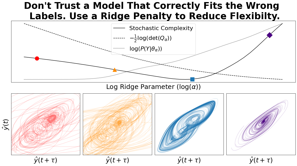
We derive a penalty strength criterion for ridge regression using stochastic complexity,
which is a refined variant of the minimum description length principle. Since stochastic
complexity doesn’t typically account for the effect of regularisation on complexity, despite
its ability to simplify models, we are required to make a slight modification to the un-
derlying coding scheme. Our scheme makes use of a weighted ensemble of regularised
model fits rather than a mixture of maximum likelihood estimates. Under this modification,
regularisation is interpreted as reducing model complexity by constraining flexibility. In
the case of ridge regression, the complexity penalty term that we derive can be expressed
analytically as the log determinant of the residual operator. We demonstrate the effect of
this complexity penalty by fitting a linear readout to a reservoir computer.
Keywords:
description length
; model selection
; information theory
; stochastic complexity
; regularisation
; ridge regression
1. Introduction
We approach the problem of selecting a regularisation strength for ridge regression with the intent of producing the simplest generalised linear model (GLM). This complexity-based approach is particularly relevant since the popularity of GLMs stems, in part, from their simplicity as a model class [1,2,14,22,43]. They are often used to identify and characterise relationships from data in fields like medicine [6], dietary science [7], economics [8,9] and sociology [10,11] . Such applications lie in accordance with Occam’s razor principle, which tells us to seek simple explanations, or in this case, simple model classes.
In these endeavours, it is common to use some form of regularisation in the fitting process, like an L1 ridge penalty. In the case of ridge regularisation, the penalty term stabilises the matrix inverse under multicollinearity of input variables [12,13,14] and improves generalisation to new data by reducing model variance at the expense of increased model bias [15,16,17]. The application of regularisation also further reduces the complexity of linear models. This makes it possible to choose the regularisation strength that minimises model complexity.
In this paper, we measure complexity in terms of stochastic complexity [18], which is a refined variant of the minimum description length principle [19] (MDL). The stochastic complexity of a model is directly related to its flexibility. When used for model selection, it suggests that we should hesitate to choose a model class that fits our dataset well if it also provides good fits to unrelated datasets using the same predictors. While regularisation constrains flexibility and produces simpler models, this is not directly accounted for by stochastic complexity. As such, the purpose of this paper, as well as deriving a ridge strength criterion, is to demonstrate a method for determining the effect of regularisation on the stochastic complexity of a model. Our method makes use of a novel interpretation of stochastic complexity’s underlying coding scheme in order to directly account for the constraint imposed by regularisation on model flexibility.
Our work is organised as follows: In Section 2, we provide an overview of stochastic complexity, including an explanation of the typical underlying coding scheme. In Section 3 we discuss our method for modifying this scheme to account for regularisation. In Section 4 we derive an analytical form for the stochastic complexity of a linear model fitted by ridge regression using our modified scheme. We also present our ridge penalty selection criterion. In Section 5 we compare our criterion with several other information-theoretic criteria. In particular, we note that our work is closely related to that of Dwivedi et al [20] who recently used luckiness normalised maximum likelihood [21] (LNML) for ridge strength selection. Their approach produces a different selection criterion, which stems from a different interpretation of regularisation’s effect on complexity. In Section 6 we use our criteria to train linear readouts with the example of reservoir computing. In Section 7, we conclude with a discussion and summary.
2. Background into Stochastic Complexity and the Minimum Description Length Principle
The premise behind MDL is that models compress information. This is done by making use of a parametric model class to derive a coding scheme for possible data sets. The shorter the encoding of the dataset we wish to model under the scheme we derive, the better the compression achieved by the model. For example, in classical two-part MDL, the scheme is to first encode our model parameters and then to encode the errors that the model makes using these parameters. The best models, according to two-part MDL, minimise the combined lengths of their error and parameter codes.
The coding scheme assumed by stochastic complexity is more abstract. No one set of model parameters is used. Instead, a probability is assigned to each potential dataset Y from the set of possibilities using a weighted ensemble of parameterisations from the same model class . If we denote the weighting associated with each parametrisation in the ensemble as , then the probability assigned by the resulting ensemble would be equivalent to the marginal probability under as a prior
Importantly, the ensemble weightings are chosen deterministically based on the model class. This is what enables the resulting code to be deciphered and makes stochastic complexity a valid description length. Under the stochastic complexity scheme, ensemble weights are chosen before the dataset Y is known in the way that minimises regret for the worst possible scenario of Y. This regret is the difference between the length of code assigned to Y by the weighted ensemble (which we denote by ) and the shortest length that could be used to encode Y with any other ensemble. Under the lower bound for efficiency given by Shannon’s source coding theorem, these code lengths are negative log probabilities . Since the best ensemble for encoding any particular dataset Y is just its maximum likelihood estimate , the worst-case regret which we seek to minimise by choice of weightings is the following
The weightings that minimise this worst-case regret are those that induce proportionality to the maximum likelihood estimate (). This means that we can work directly with without ever actually determining the optimal weightings. Under proportionality, regret is constant across all datasets . The constant of proportionality c must be the sum of all maximum likelihood estimates in order for it to induce a probability distribution that integrates to one. The probability of Y under is therefore given as follows
When we work with continuous data, and therefore an infinite set of possible datasets , the ensemble weights become difficult to determine. They have been shown [22,23], to approach the Jeffreys prior [24] for large datasets under certain conditions [25]. However, we are not required to determine the ensemble weights since proportionality still holds, and we can again work directly with . In the case of continuous data, the stochastic complexity makes use of the integral version for
Notice that stochastic complexity can be broken into two terms, the first being the model’s negative log likelihood. The other term measures the complexity of the parametric model class
and functions as the penalty term in model selection. This penalty directly measures flexibility and it lends stochastic complexity an important intuition beyond its meaning as a code length. It tells us not to trust models that fit the data well if they can also provide good fits to unrelated data using the same predictors.
3. The effect of Regularisation on Complexity
The role of model regularisation on stochastic complexity can potentially be interpreted in different ways. Our interpretation is to directly consider the effect of regularisation on the flexibility of the model class. This follows on from the intuitive meaning of stochastic complexity described in the previous section: that we should have more confidence in our regularised model if the regularisation applied prevents the model from easily fitting unrelated datasets using the same predictors.
Rather than building a weighted ensemble of maximum likelihood estimates, we build a weighted ensemble of regularised fits. The weightings of this ensemble will depend on the regularisation strength . We select the weightings such that the probability assigned by the ensemble is proportional to the probability assigned by the regularised fit , which again minimises worst-case regret. This regret, which we now denote by , because of its dependence on the regularisation strength , is still the length of code that could have been saved had the parameter fit for the dataset been known ahead of time. The only difference is that this parameter fit is now the set of regularised parameters and not the maximum likelihood estimate
Assuming that the encoder and decoder also know the regularisation strength ahead of time, the resulting ensemble weights can be calculated by the decoder, allowing them to decipher any subsequent encoding. Under this interpretation, which therefore describes a valid description length, the stochastic complexity of a dataset Y becomes the following
One benefit of this approach is its generalisability. It can be applied directly to other methods for fitting and regularising parameters. Another benefit is the fairness of the comparison it draws between regularisation techniques. One technique can be compared with another based purely on how much each restricts the flexibility of the model class. The caveat, which is not unique to our approach, is that to derive an analytical value for stochastic complexity, we still need an analytical form for the model likelihood when regularisation is applied.
4. Deriving a Ridge Penalty to Minimise Stochastic Complexity
In the case of regression with a known state matrix X, the parametric model class is the multivariate normal distribution . This is the model class for which the regression solution provides the maximum likelihood estimate. From a Bayesian perspective, the ridge penalty comes from maximising the posterior with the added assumption of a normal prior over the parameters. However, it is not strictly necessary to assume a prior over the parameters in order to calculate stochastic complexity. We only need to know the probability of each dataset given the regularised parameter fit . According to our model class, that probability is the following
Fortunately, an analytical form for this probability exists. First, we can express the ridge regression solution in terms of the penalty , the state matrix X and the dataset Y. It is given by . This means that an analytical form for the mean square error, which we denote by , also exists
In the expression above, n refers to the length of Y.
To find the stochastic complexity penalty term, we integrate the resulting probability over the space of all possible datasets. For continuous datasets of length n, this space is and the penalty is the following
We can write the value of this integral in terms of the determinant of
or in terms of the eigenvalues of the design matrix , which we denote by
This penalty describes how well we can fit various possible datasets using regression with a ridge constant of and a gram matrix that has the given spectrum . Lastly, we need the other component of the stochastic complexity, which is the log likelihood of Y under its own parameter fit . Together, the stochastic complexity becomes the following function of the ridge penalty:
The constant term, which we ignore because it is irrelevant for our purpose, is .
Calculating the stochastic complexity requires choosing a variance for the multivariate Gaussian used in our coding scheme. This is also the case for various other ridge penalty criteria [26,27]. A typical method for doing so in the under-parameterised case () is to estimate in terms of the adjusted mean square error of the linear regression solution . A more robust method, which is not limited to the under-parametrised case, is provided by Liu et al [28]. They suggest approximating by the following
Our formulation for optimising the ridge penalty passes two sanity checks that we can construct from our understanding of ridge regression. Firstly, the optimal penalty scales correctly with the terms of the state matrix. If X is multiplied by a scalar , the optimal ridge penalty should scale with its square , since this leaves the projection matrix unchanged. This is the case. Multiplying the state matrix X by a scalar adds a trivial constant to the penalty term and maps to . Secondly, since the penalty term is a measure of model flexibility, it should only depend on the unique, non-zero columns in X. This is also true. Duplicate columns, or columns of zeros, add eigenvalues of zero to the spectrum and these do not contribute to the penalty term.
5. Alternative Approaches
In Section 3 we accounted for regularisation by devising a coding scheme from an ensemble of regularised parameter fits. An alternative approach is to build the ensemble from maximum posterior likelihood estimates after assuming a prior distribution over parameter space. This is similar to the way that luckiness normalised maximum likelihood (LNML) assumes a so-called `luckiness function’ to derive a model score
Dwivedi et al [20] chose to be a Gaussian density for ridge regression
This choice is meaningful because a Gaussian prior over the parameters produces a posterior likelihood which is maximal at the ridge regression solution. The numerator and denominator therefore both measure posterior likelihoods. The corresponding description length assigned by Dwivedi et al, which we denote by and provide below, is similar to our own, but includes an additional log parameter likelihood term
The approach taken by Dwivedi et al can be generalised to any regularisation techniques that offer a Bayesian interpretation. The luckiness score would simply be replaced with whatever prior distribution is implicitly assumed over the parameters.
The MDL-inspired approach taken by Silhavy et al [29] makes use of a two-part coding scheme. They take the description length found for linear regression by Giurcaneanu et al [30] and consider the additional cost of encoding the ridge parameter (or Lasso parameter). It should be noted, that Giurcaneanu et al found the description length for linear regression under a different framing of the model class. They encode the error variance and then use the variance to encode the errors . As such, Silhavy et al’s method for choosing an MDL ridge parameter is quite different from our own. They seek to minimise the following criterion
It should also be noted that the major objective of Silhavy et al’s work was to apply MDL to multi-criteria decision analysis. This means seeking a tradeoff between model complexity and a combination of various performance measures. In this paper, we only deal with a single objective, which is model log likelihood (effectively mean square model error).
Other information criteria, like the Akaike [31] and Bayesian [32] Information Criteria (AIC and BIC respectively), can also be used to choose a ridge strength if the number of model parameters is replaced with the number of effective degrees of freedom which has dependence on [33,34]. The commonly used measure of effective degrees of freedom is the trace of the projection matrix [35,36]. This results in the modified AIC and BIC criteria provided below
6. Fitting a Reservoir Computer
As a proof of concept, we use our ridge penalty criterion to select a penalty strength for fitting reservoir computer readouts. Reservoir computers are high-dimensional dynamical systems that become conditionally stable when driven by an input signal. Their dynamic response is mapped to the future state of the input with a linear readout. This mapping is possible because the reservoir state-space becomes a time-delay embedding-space of the driving time series [37] according to the echo-state property [38,39], which reservoirs must satisfy. Reservoir readouts are often fitted with ridge regression [40,41,42] and their complexity is a subject of interest [43,44,45,46]. In particular, we use echo-state networks [47] as our reservoirs and perform time series prediction on Lorenz-96 [48]. Our exact method is detailed in the Appendix along with a description of echo-state networks.
The average generalisation error for one-step prediction of Lorenz-96 is compared with network size in Figure 1. The ridge penalty chosen according to stochastic complexity (in black) produces smaller generalisation error on average than any fixed penalty magnitude. This is true across a range of network sizes and suggests that our method leads to sensible choices for the ridge parameter. Our criterion also achieves comparable results to some of the alternative approaches mentioned in Section 5, and performs comparatively well on large networks. This is demonstrated in Figure 2. It should be noted that the relative strength of the model complexity term is dependent on the value of for these methods, which we choose to be the smaller of the two values described in Section 4
The first of these values is always positive and defined, since the length of the training time series is 1200 points and the largest network has 1096 nodes.
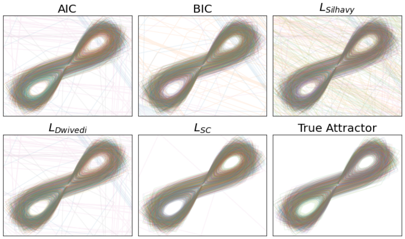
Qualitative comparisons of reconstruction ability are also provided in Figure 3 and Figure 4. This time, echo-state networks are trained for one-step-ahead prediction of the Lorenz system. Individual trajectories in each subplot are generated by continuously driving echo-state networks with their own past predictions. These predictions depend on output coefficients, which in turn depend on the ridge strength selected by each criterion. All criteria tend to produce reconstructions that are qualitatively similar to the Lorenz attractor when networks and prediction step sizes are small. This indicates that the ridge strengths they select tend to be appropriate for capturing the underlying dynamics. For example, the reconstruction composites in Figure 3 are made using 200 node networks trained at a sampling rate of s. On the other hand, ridge strengths selected by stochastic complexity appear to produce reasonable reconstructions more often when networks and step sizes are larger. This is the case in Figure 4 where predictions are made using 800 node networks and a step size of s.
7. Summary and Comments
We have proposed a selection criterion for the choice of penalty strength in ridge regression. In the process, we have demonstrated an application of stochastic complexity to a common problem. This required that we devise a model encoding scheme in accordance with the typical stochastic complexity scheme, but which is sensitive to the application of regularisation. Our scheme suggests that we can consider the reduction in model complexity induced by regularisation as a constraint on model flexibility. We believe that this result is consistent with the intuitive message espoused by stochastic complexity - that we should be hesitant in choosing a model class that fits our data well if it provides good fits to unrelated datasets using the same predictors. Regularisation should ease our hesitancy by preventing our model from easily fitting these unrelated datasets.
The ridge penalty selection criterion that we derived produced promising results when used to fit linear readouts for echo-state networks. Moreover, the interpretation of stochastic complexity from which it was derived is generalisable to other regularisation techniques and different model classes.
Author Contributions
Conceptualization, A.M.; methodology, A.M.; software, A.M.; validation, A.M., D.W. and M.S.; formal analysis, A.M.; investigation, A.M.; resources, A.M.; data curation, A.M.; writing—original draft preparation, A.M.; writing—review and editing, A.M., D.W. and M.S.; visualization, A.M.; supervision, D.W. and M.S.; project administration, A.M., D.W. and M.S. All authors have read and agreed to the published version of the manuscript.
Funding
Not applicable yet.
Institutional Review Board Statement
Not applicable.
Informed Consent Statement
Not applicable.
Data Availability Statement
The data that support the findings of this study are openly available in the github repository Stochastic_Complexity_for_RR, accessible at https://github.com/antony-mizzi/Stochastic_Complexity_for_RR.
Acknowledgments
A.M. was supported by the Australian Government RTP scholarship at the University of Western Australia. M.S. and D.M.W. are supported by the ARC Discovery Grant (No. DP200102961), funded by the Australian Government.
Conflicts of Interest
The authors declare no conflicts of interest.
Abbreviations
The following abbreviations are used in this manuscript:
| GLM | Generalised Linear Model |
| MDL | Minimum Description Length |
| LNML | Luckiness Normalised Maximum Likelihood |
| AIC | Akaike Information Criterion |
| BIC | Bayesian Information Criterion |
| ESN | Echo-State Network |
Appendix A
Appendix A.1
Echo-state networks (ESNs) are a specific type of reservoir. They consist of a network and a set of input weights and behave like the recurrent part of a recurrent neural network. At each time step, the network is driven according to the value of the time series . The network state updates according to the governing equation
Unlike recurrent neural networks, the adjacency matrix A, input connections and node biases b all remain untrained. The activation function f, which in our case is the hyperbolic tangent , introduces non-linearity. Predictions at each time step are given by the linear combination of node values with parameters determined from ridge regression . We train echo-state networks for one-step-ahead prediction. In this case, X is the matrix with a row of and Y is the vector with a entry of .
In the experiments performed in Section 6, every sample involves a new ESN architecture and a newly generated time series. We generate the network adjacency A as a weighted Watts-Strogatz network with a connectivity of 6 weightings drawn from the standard normal. The adjacency matrix is then normalised to have a spectral radius of which is sampled uniformly between and . Input connection strengths are sampled from a Gaussian with zero mean and a standard deviation of . We do not use node biases ().
For Figure 1 and Figure 2 the driving time series consists of 1200 points generated from a Runge-Kutta (RK4) integration of Lorenz-96 with a sampling rate of s. Lorenz96 is a high-dimensional dynamical system with a Lyapunov time that we calculate to be about s using the method in [49]. It has a governing set of equations detailed below in eq Appendix A.1, and we use the hyperparameters .
Note that in this equation, is the same as .
For the time delay embedding plots (Figure 3 and Figure 4), we instead train the reservoir at one-step prediction using 1200 points from the Lorenz system. The governing equations of this system are provided below. We use standard hyperparameters for which we calculate the Lyapunov time to be around seconds.
The trajectories shown in Figure 3 and Figure 4 are generated autonomously. This means that rather than driving ESNs by an external signal, we instead drive them at each time step by their previous prediction. Effectively, their predictions are an Eulerian integration of the following system of equations
This autonomous prediction is continued for a fixed duration of 200 time steps. For each predicted trajectory , We graph against in Figure 3 and against in Figure 4. Both plots are comprised of 50 different trajectories, each of which is produced by a different ESN architecture trained on a different time series. The same 50 architectures and time series are used in each subplot.
References
- Judd, K.; Mees, A. On selecting models for nonlinear time series. Phys. D. Nonlinear Phenom. 1995, 82, 426–444. [Google Scholar] [CrossRef]
- Myers, R.H.; Montgomery, D.C.; Vining, G.G.; Robinson, T.J. Generalized Linear Models: With Applications in Engineering and the Sciences; John Wiley & Sons, 2012. [Google Scholar]
- Fan, L.; Miao, Z.; Shah, S.; Cheng, Y.; Rose, J.; Huang, S.H.; Pal, B.; Xie, X.; Modi, N.; Wang, S.; Zhu, S. Real-world 20-Hz IBR subsynchronous oscillations: Signatures and mechanism analysis. IEEE Trans. Energy Convers. 2022, 37, 2863–2873. [Google Scholar] [CrossRef]
- Nozari, E.; Bertolero, M.A.; Stiso, J.; Caciagli, L.; Cornblath, E.J.; He, X.; Mahadevan, A.S.; Pappas, G.J.; Bassett, D.S. Macroscopic resting-state brain dynamics are best described by linear models. Nat. Biomed. Eng. 2024, 8, 68–84. [Google Scholar] [CrossRef] [PubMed]
- Gonzalez-Lopez, M.E.; Laureano-Anzaldo, C.M.; Pérez-Fonseca, A.A.; Arellano, M.; Robledo-Ortiz, J.R. A critical overview of adsorption models linearization: Methodological and statistical inconsistencies. Sep. Purif. Rev. 2022, 51, 358–372. [Google Scholar] [CrossRef]
- Schneider, A.; Hommel, G.; Blettner, M. Linear regression analysis: Part 14 of a series on evaluation of scientific publications. Dtsch. ÄRzteblatt Int. 2010, 107, 776–782. [Google Scholar]
- Zhang, F.; Tapera, T.M.; Gou, J. Application of a new dietary pattern analysis method in nutritional epidemiology. BMC Med. Res. Methodol. 2018, 18, 119. [Google Scholar] [CrossRef]
- Hellwig, Z. Linear Regression and its Application to Economics; Elsevier, 2014. [Google Scholar]
- Peters, G. A linear forecasting model and its application to economic data. J. Forecast. 2001, 20, 315–328. [Google Scholar] [CrossRef]
- Torres, A.F.C.; Akbaritabar, A. The hegemonic use of linear models in quantitative social sciences. Bull. Sociol. Methodol. Bull. De Méthodologie Sociol. 2025, 167, 78–95. [Google Scholar] [CrossRef]
- Mize, T.D. Best practices for estimating, interpreting, and presenting nonlinear interaction effects. Sociol. Sci. 2019, 6, 81–117. [Google Scholar] [CrossRef]
- Luqman, M.; Bhatti, S.H.; Aydin, D.; Jamil, M. Addressing multicollinearity in general linear model: A novel approach for ridge parameter with performance comparison. PLoS ONE 2025, 20, e0335072. [Google Scholar] [CrossRef] [PubMed]
- Hoerl, A.E.; Kennard, R.W. Ridge regression—1980: Advances, algorithms, and applications. Am. J. Math. Manag. Sci. 1981, 1, 5–83. [Google Scholar] [CrossRef]
- Conniffe, D.; Stone, J. A critical view of ridge regression. J. R. Stat. Soc. Ser. D. (The Statistician) 1973, 22, 181–187. [Google Scholar] [CrossRef]
- Wu, D.; Xu, J. On the optimal weighted ℓ2 regularization in overparameterized linear regression. Adv. Neural Inf. Process. Syst. 2020, 33, 10112–10123. [Google Scholar]
- Gillariose, J.; Joseph, J.; Chesneau, C. Lasso and ridge regression: A comprehensive review of applications and developments in machine learning. Int. J. Data Sci. Anal. 2026, 21, 7. [Google Scholar] [CrossRef]
- Reid, S.; Grudic, G. Regularized linear models in stacked generalization. In Proceedings of the International Workshop on Multiple Classifier Systems; Springer: Berlin/Heidelberg, Germany, 2009; pp. 112–121. [Google Scholar]
- Rissanen, J. Stochastic complexity. J. R. Stat. Soc. Ser. B (Methodological) 1987, 49, 223–239. [Google Scholar] [CrossRef]
- Rissanen, J. Modeling by shortest data description. Automatica 1978, 14, 465–471. [Google Scholar] [CrossRef]
- Dwivedi, R.; Singh, C.; Yu, B.; Wainwright, M. Revisiting minimum description length complexity in overparameterized models. J. Mach. Learn. Res. 2023, 24, 1–59. [Google Scholar]
- Grünwald, P.D. The Minimum Description Length Principle; MIT Press, 2007. [Google Scholar]
- Clarke, B.S.; Barron, A.R. Information-theoretic asymptotics of Bayes methods. IEEE Trans. Inf. Theory 2002, 36, 453–471. [Google Scholar] [CrossRef]
- Grunwald, P. The Minimum Description Length Principle and Reasoning Under Uncertainty. Ph.D. Thesis, University of Amsterdam, Amsterdam, Netherlands, January 1998. [Google Scholar]
- Jeffreys, H. An invariant form for the prior probability in estimation problems. In Proceedings of the Royal Society of London. Series A: Mathematical and Physical Sciences, London, UK, 24 September 1946; 186, pp. 453–461. [Google Scholar]
- Kontkanen, P.; Buntine, W.; Myllymäki, P.; Rissanen, J.; Tirri, H. Efficient computation of stochastic complexity. In Proceedings of the Ninth International Conference on Artificial Intelligence and Statistics, Key West, Florida, USA, 21 March 2003; Society for Artificial Intelligence and Statistics; pp. 233–238. [Google Scholar]
- Kibria, B. G. More than hundred (100) estimators for estimating the shrinkage parameter in a linear and generalized linear ridge regression models. J. Econom. Stat. 2022, 2, 233–252. [Google Scholar]
- Cule, E.; Do Iorio, M. Ridge regression in prediction problems: automatic choice of the ridge parameter. Genet. Epidemiol. 2013, 37, 704–714. [Google Scholar] [CrossRef]
- Liu, X.; Zheng, S.; Feng, X. Estimation of error variance via ridge regression. Biometrika 2020, 107, 481–488. [Google Scholar] [CrossRef]
- Silhavy, P.; Hlaváčková-Schindler, K.; Silhavy, R. Minimum description length and multi-criteria decision analysis in predictive modeling. IEEE Access 2025, 13, 19388–19407. [Google Scholar] [CrossRef]
- Giurcăneanu, C.D.; Razavi, S.A.; Liski, A. Variable selection in linear regression: Several approaches based on normalized maximum likelihood. Signal Process. 2011, 91, 1671–1692. [Google Scholar] [CrossRef]
- Akaike, H. A new look at the statistical model identification. IEEE Trans. Autom. Control 1974, 19, 716–723. [Google Scholar] [CrossRef]
- Schwarz, G. Estimating the dimension of a model. Ann. Stat. 1978, 6, 461–464. [Google Scholar] [CrossRef]
- Van Le, C. How to choose tuning parameters in lasso and ridge regression? Asian J. Econ. Bank. 2020, 4, 61–76. [Google Scholar]
- Flynn, C.J.; Hurvich, C.M.; Simonoff, J.S. Efficiency for regularization parameter selection in penalized likelihood estimation of misspecified models. J. Am. Stat. Assoc. 2013, 108, 1031–1043. [Google Scholar] [CrossRef]
- Dijkstra, T.K. Ridge regression and its degrees of freedom. Qual. Quant. 2014, 48, 3185–3193. [Google Scholar] [CrossRef]
- Boonstra, P.S.; Mukherjee, B.; Taylor, J.M. A small-sample choice of the tuning parameter in ridge regression. Stat. Sin. 2015, 25, 1185–1206. [Google Scholar] [CrossRef]
- Duan, X.-Y.; Ying, X.; Leng, S.-Y.; Kurths, J.; Lin, W.; Ma, H.-F. Embedding theory of reservoir computing and reducing reservoir network using time delays. Phys. Rev. Res. 2023, 5, L022041. [Google Scholar] [CrossRef]
- Jaeger, H. Erratum note for the techreport: The “echo state” approach to analysing and training recurrent neural networks. Technical Report, 2010.
- Yildiz, I.B.; Jaeger, H.; Kiebel, S.J. Revisiting the echo state property. Neural Netw. 2012, 35, 1–9. [Google Scholar] [CrossRef]
- Panahi, S.; Zhai, Z.-M.; Haile, M.; Lai, Y.-C. Neuromorphic reservoir computing. Chaos An. Interdiscip. J. Nonlinear Sci. 2025, 35. [Google Scholar] [CrossRef]
- Cucchi, M.; Abreu, S.; Ciccone, G.; Brunner, D.; Kleemann, H. Hands-on reservoir computing: A tutorial for practical implementation. Neuromorphic Comput. Eng. 2022, 2, 032002. [Google Scholar] [CrossRef]
- Kent, R.; Lienhard, B.; Lafyatis, G.; Gauthier, D.J. Superconducting qubit readout using next-generation reservoir computing. Phys. Rev. Appl. 2026, 25, 044009. [Google Scholar] [CrossRef]
- Abdalla, M.; Zrounba, C.; Cardoso, R.; Jimenez, P.; Ren, G.; Boes, A.; Mitchell, A.; Bosio, A.; O’Connor, I.; Pavanello, F. Minimum complexity integrated photonic architecture for delay-based reservoir computing. Opt. Express 2023, 31, 11610–11623. [Google Scholar] [CrossRef] [PubMed]
- Dale, M.; Dewhirst, J.; O’Keefe, S.; Sebald, A.; Stepney, S.; Trefzer, M.A. The role of structure and complexity on reservoir computing quality. In Proceedings of the International Conference on Unconventional Computation and Natural Computation, Tokyo, Japan, 3-7 June2019; Springer; pp. 52–64. [Google Scholar]
- Zeng, Y.; Li, Z.; Gao, X.; Cheng, M. Optical chaos shift keying communication system via neural network-based signal reconstruction. Nonlinear Dyn. 2025, 113, 32849–32863. [Google Scholar] [CrossRef]
- Fong, R.S.; Li, B.; Tino, P. Universality of real minimal complexity reservoir. In Proceedings of the AAAI Conference on Artificial Intelligence, Philadelphia, Pennsylvania, USA, 25 February - 4 March 2025; Vol. 39, pp. 16622–16629. [Google Scholar]
- Jaeger, H. The “echo state” approach to analysing and training recurrent neural networks—with an erratum note. GMD Technical Report 148, 2001.
- Lorenz, E.N. Predictability: A problem partly solved. Proceedings of Seminar on Predictability, Shinfield Park, Reading, UK, 4-8 September 1996; Vol. 1, pp. 1–18. [Google Scholar]
- Benettin, G.; Galgani, L.; Giorgilli, A.; Strelcyn, J.M. Lyapunov characteristic exponents for smooth dynamical systems and for Hamiltonian systems; a method for computing all of them. Meccanica 1980, 15, 9–20. [Google Scholar] [CrossRef]
Figure 1.
Reservoir performance compared with network size for different choices of regularisation strength. The black line represents the performance achieved by the ridge strength that minimises our selection criterion. All results are averaged over 200 samples and the error bounds indicate twice the standard deviation of bootstrap means.
Figure 1.
Reservoir performance compared with network size for different choices of regularisation strength. The black line represents the performance achieved by the ridge strength that minimises our selection criterion. All results are averaged over 200 samples and the error bounds indicate twice the standard deviation of bootstrap means.
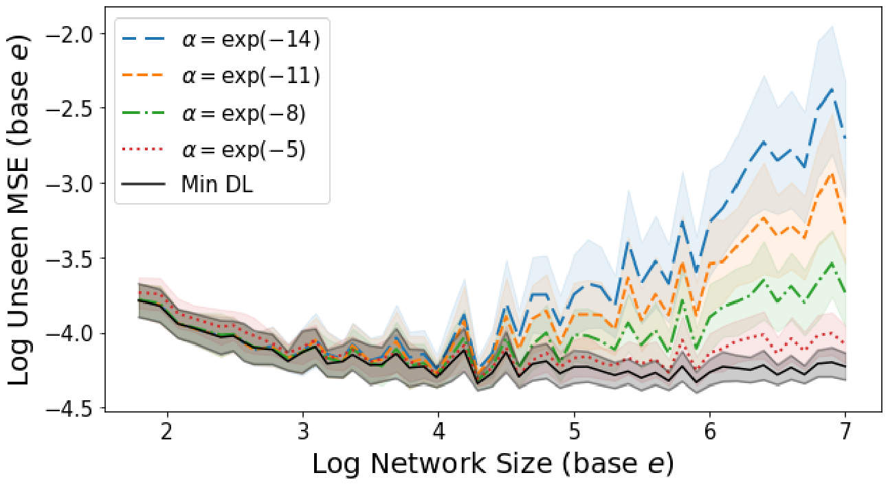
Figure 2.
Reservoir performance compared with network size using ridge parameters selected by information theoretic criteria. Our criterion is graphed in black, and the other criteria are described in Section 5. All results are averaged over 200 samples, and the error bounds indicate twice the standard deviation of bootstrap means.
Figure 2.
Reservoir performance compared with network size using ridge parameters selected by information theoretic criteria. Our criterion is graphed in black, and the other criteria are described in Section 5. All results are averaged over 200 samples, and the error bounds indicate twice the standard deviation of bootstrap means.
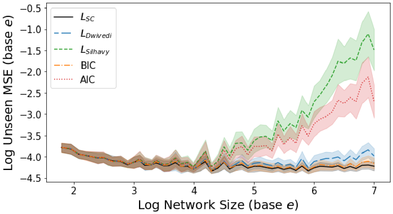
Figure 3.
Composite time-delay embedding plots made from 50 trajectories autonomously reconstructed by echo-state networks. Each trajectory consists of 200 points predicted by a different network trained on a different integration of Lorenz. Each network has 200 nodes, and the prediction step size is s. The plot in the bottom right corner contains 50 trajectories from the Lorenz attractor for comparison.
Figure 3.
Composite time-delay embedding plots made from 50 trajectories autonomously reconstructed by echo-state networks. Each trajectory consists of 200 points predicted by a different network trained on a different integration of Lorenz. Each network has 200 nodes, and the prediction step size is s. The plot in the bottom right corner contains 50 trajectories from the Lorenz attractor for comparison.
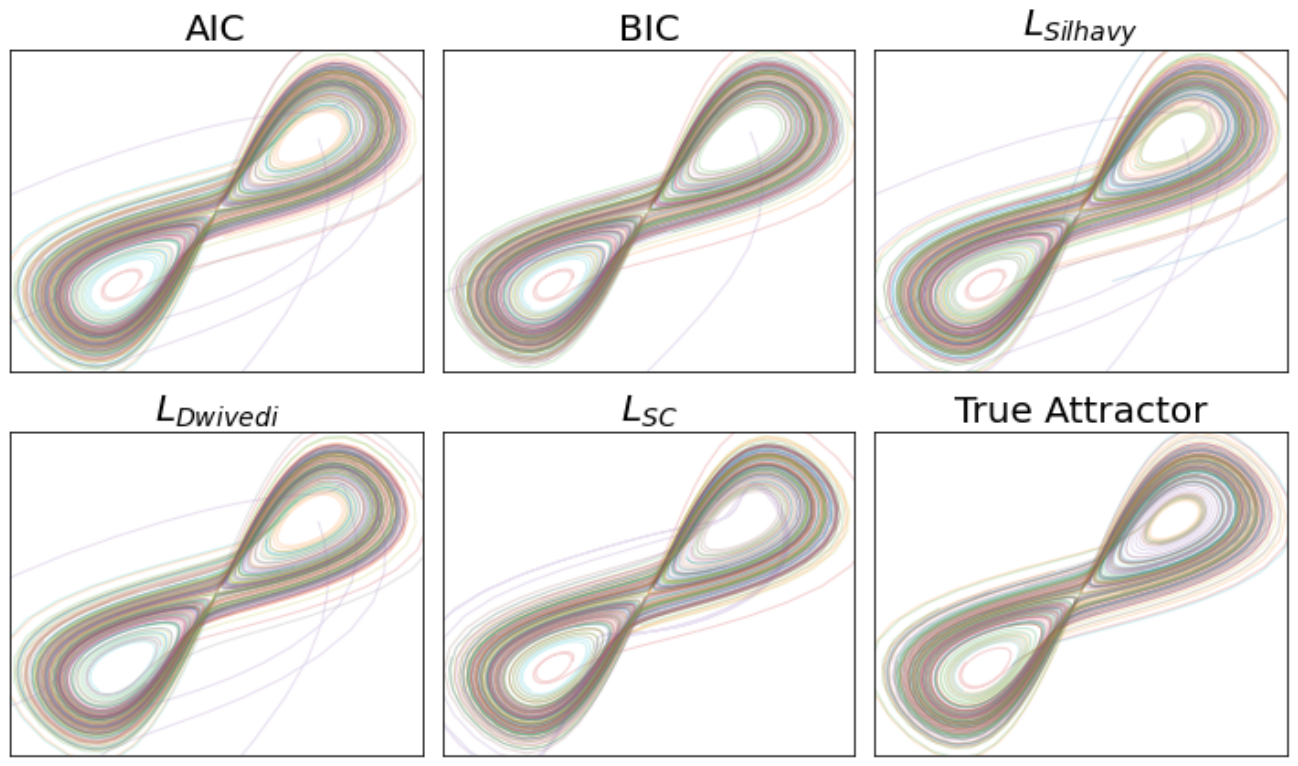
Figure 4.
Composite time-delay embedding plots, this time using 800 node networks and a prediction step size of s.
Figure 4.
Composite time-delay embedding plots, this time using 800 node networks and a prediction step size of s.
Disclaimer/Publisher’s Note: The statements, opinions and data contained in all publications are solely those of the individual author(s) and contributor(s) and not of MDPI and/or the editor(s). MDPI and/or the editor(s) disclaim responsibility for any injury to people or property resulting from any ideas, methods, instructions or products referred to in the content. |
© 2026 by the authors. Licensee MDPI, Basel, Switzerland. This article is an open access article distributed under the terms and conditions of the Creative Commons Attribution (CC BY) license (http://creativecommons.org/licenses/by/4.0/).
Copyright: This open access article is published under a Creative Commons CC BY 4.0 license, which permit the free download, distribution, and reuse, provided that the author and preprint are cited in any reuse.


