
Submitted:
07 May 2026
Posted:
11 May 2026
You are already at the latest version
Abstract
This article analyzes the impact of agricultural support measures on food import dependency for a 52-country sample from 1985 to 2017 using databases from the World Bank, the Center for Systemic Peace and the Groningen Center for Growth and Development. We apply a continuous treatment effect and control for endogeneity to describe the extent of food import dependency in response to domestic support for agriculture. Our results show strong evidence of heterogeneous impacts on aggregate food import dependency at different levels of political aid intensity. Estimates of dose-response functions confirm that countries providing moderate support to agriculture tend to do better in reducing their use of agri-food imports.
Keywords:
food import dependency
; trade
; agricultural support
; continuous treatment effect
; doseresponse
; developing countries
1. Introduction
1.1. Context
Classical international trade theory does not predict that trade openness mechanically reduces food trade deficits. Rather, the theory of comparative advantage emphasizes welfare and income gains from trade, which may reduce the share of income spent on food and improve access to food through imports. In economies with limited agricultural resources, however, trade liberalization may be associated with higher food import dependence, especially when free trade replaces restrictive agricultural import policies. Consequently, the relationship between trade, agricultural policies, and food import dependence remains theoretically ambiguous [9]. This ambiguity suggests that the effect of trade openness on food import dependence crucially depends on domestic agricultural support policies and their intensity, which motivates our empirical investigation.
Importantly, food import dependence is not interpreted here as an inherently undesirable outcome, but rather as an equilibrium outcome reflecting countries’ structural characteristics, policy choices, and exposure to international markets. Food import dependence should not be interpreted as food insecurity. Food trade has long been recognized as a key mechanism for smoothing consumption and mitigating food insecurity, particularly in the presence of weather-related supply shocks. By integrating local markets into broader trading networks, food imports reduce exposure to local yield shocks. Burgess and Donaldson [22] show that the dramatic reduction in transport costs brought by railroads in India substantially lowered famine incidence and weakened the link between local weather shocks and food availability. In this sense, food import dependence reflects exposure to international markets rather than food insecurity per se. While such exposure can enhance food security by stabilizing supplies, it may also increase vulnerability to external price shocks, foreign exchange constraints, or policy disruptions. This dual role of food imports underscores the importance of examining how domestic agricultural support policies condition the relationship between trade openness and food import dependence.
Food import dependence is also shaped by deep structural factors such as factor endowments, geography, and climatic constraints. Landlocked countries, small island states, or countries located in temperate zones face inherent limitations in producing certain food products, irrespective of agricultural support policies. In such contexts, some degree of food import dependence is unavoidable unless agricultural support generates substantial technological change and productivity gains. Despite the stabilizing role of food trade, several authors have expressed skepticism toward agricultural development strategies that prioritize export promotion in developing countries. Such strategies, when focused on a limited set of export-oriented crops, may increase dependence on food imports and heighten vulnerability to external shocks, with potential adverse implications for food security [9,40]. In this context, agricultural support policies play a central role, as they can either reinforce import dependence or, alternatively, create conditions under which export revenues are used to support domestic food production.
Nevertheless, other contributions emphasize that export earnings may relax foreign exchange constraints and finance investments in domestic food production, thereby mitigating food import dependence [38,52]. Lamb [52] concludes that a country’s export earnings could enable it either to import more food products or to import intermediate goods needed to increase domestic food crop productivity. In the latter case, local agricultural product promotion follows from the promotion of export crops and would help to limit dependence on food imports. In the same vein, other authors [38] have explored how the development of export crops could finance the creation of institutions to support agriculture (e.g., through investments in infrastructure, extension services, agricultural research, subsidies, etc.).
On the one hand, the literature highlights how changes in agricultural support and trade policies, often motivated by domestic price stabilization objectives, can increase countries’ exposure to international food markets. In particular, policies of food price insulation, which are generally explained by governments’ desire to reduce domestic price volatility or by loss aversion, are well documented in the literature. In this context, policies of food price insulation are well known, as are their unintended consequences in terms of magnifying price volatility at the world level. Larochez-Dupraz and Huchet-Bourdon [53], for instance, focus on how changes in the Nominal Rate of Assistance (NRA) affect the vulnerability of food security to trade, rather than on food import volumes per se. On the other hand, other contributions emphasize that export earnings may relax foreign exchange constraints and finance investments in domestic food production, thereby mitigating food import dependence [38,52].
However, agricultural support measures can be heterogeneous between countries and between regions, and this heterogeneity could affect trade results, including food imports [77]. Moreover, different farming systems imply different levels of agricultural support [77].
Based on these conclusions, one can question the role that support measures play in the food import dependencies of developing countries. To our knowledge, except for the works of Larochez–Dupraz and Huchet–Bourdon [53] and some others, very few studies have attempted to provide answers. We contribute to the literature by examining how the intensity of agricultural support policies conditions food import dependency across developing countries, recognizing that such dependency reflects both policy choices and structural constraints.
To achieve this, we estimate a dose-response function that considers endogeneity using the continuous treatment model proposed by Cerulli et al. [27]. Unlike other techniques for analyzing treatment effects [49], this model is based on an instrumental variable stepwise regression technique [27] that corrects the potential endogeneity biases that exist in the estimation of the relationship between agricultural support measures and food import dependencies in the studied countries [54]. However, one difficulty in using instrumental variables for the estimation of the endogenous treatment model is the identification of valid instruments [46]. Faced with such difficulty, the theoretical and empirical literature on the determinants of agricultural support offers instruments that can provide a solution to the endogeneity problem [6,16,39,70].
In this article, we present some stylized facts below and review the literature on the determinants of agricultural support and food security in Section 2. Section 3 illustrates the econometric framework of our study. Section 4 presents the data and the estimation strategies. Section 5 reports and discusses the results of our study. Section 6 provides the policy implications, and we conclude this work in Section 7.
1.2. Some Stylized Facts
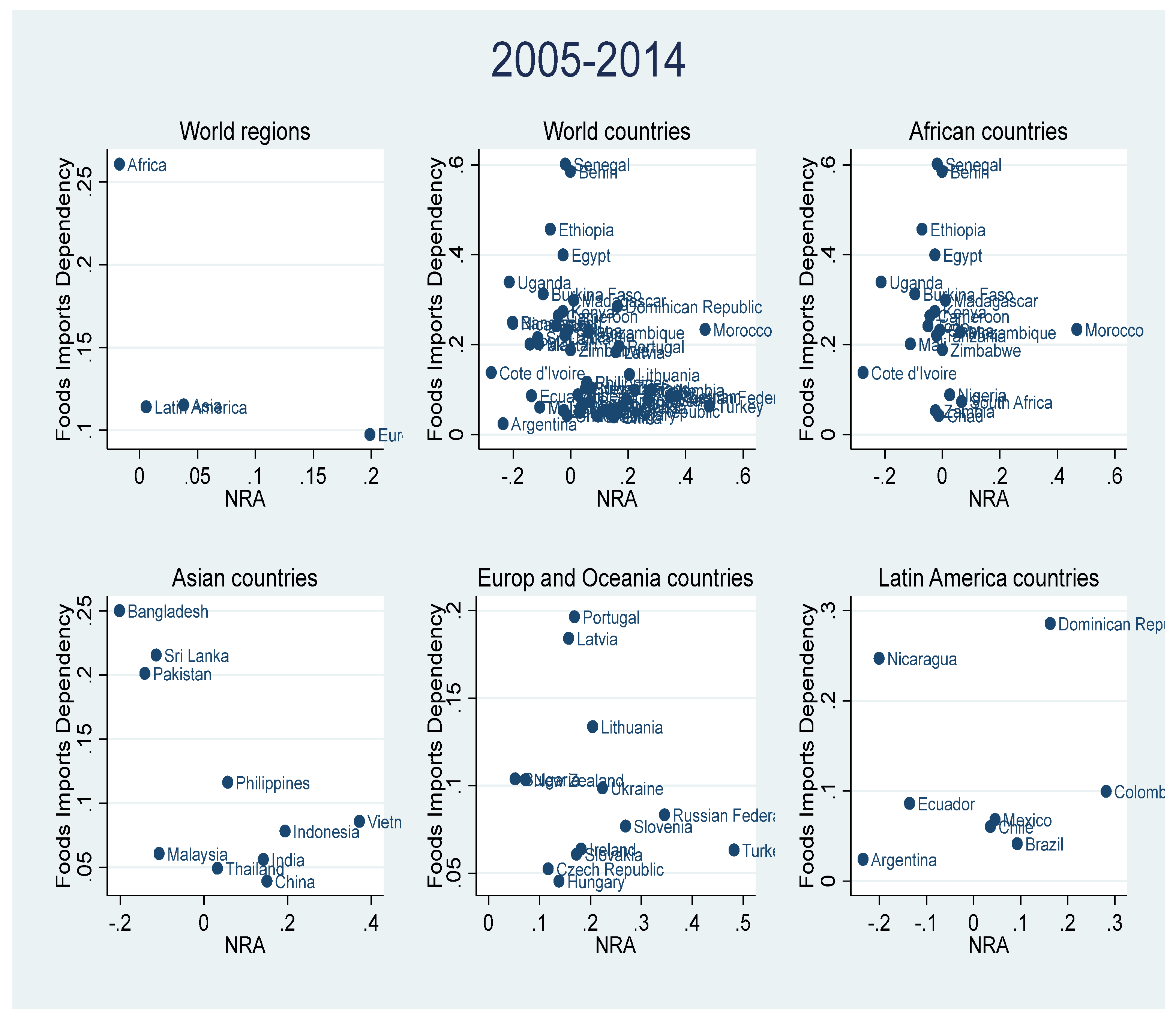
Figure A2, Figure A3 and Figure A4 (Appendix C) reveal that over the periods 1985–1994, 1995–2004, and 2005–2017, the Africa region had, on average, the lowest levels of agricultural support compared to other studied regions of the world; at the same time, the Africa region records the highest levels of food import dependencies during the same periods. The figures also show that although the average level of agricultural support in this region of the world increased over the different periods, such support has not always improved the incomes of agricultural producers (the average values of nominal rates of assistance to agriculture have remained negative over all these periods in the Africa region).
In the Latin America and Asia regions, the individual country situation is identical to that of the Africa region, although when considering the countries considered in these regions of the world overall, on average, the rates of food import dependency have remained considerably lower than those observed in Africa for the periods 1985–1994, 1995–2004 and 2005–2017 (see Figure A2, Figure A3 and Figure A4 – World Regions and Latin American Countries); Similarly, the Asia region has remained relatively less dependent on food imports than has the Latin American region over all these periods.
In the Europe and Oceania regions, agricultural assistance measures remained positive for most countries over the three periods 1985–1994, 1995–2004, and 2005–2017 (see Figure A2, Figure A3 and Figure A4 – World regions and Country Europe and Oceania). Therefore, support for agriculture consolidates the income of producers. However, at the same time, the import dependence of these countries has remained low compared to countries in other regions of the world (see Figure A2, Figure A3 and Figure A4).
These findings suggest the heterogeneity of support for agriculture among both regions and countries. Therefore, an analysis of the effects of support for agriculture on food import dependency must be considered. To accomplish that, we adopt an endogenous treatment approach based on instrumental variable techniques. Our approach postulates that macroeconomic and sociopolitical factors can explain the differences in treatments for agricultural assistance.
2. Materials and Methods
2.1. Theory
2.1.1. Determinants of Agricultural Support
Theoretical contributions in the field of political economy on institutions and democracy [2,58], the role of constitutions [60], political competition [34], and electoral institutions [20] have deepened research on the determinants of support in agriculture. For Olper [58], farmers’ voices can be better heard in an electoral democracy where interest groups are free to compete for political rents. In contrast, authoritarian regimes, which are better able to discourage the rent-seeking activities of interest groups, tax or do not support their agricultural sectors [58]. These different arguments suggest that agricultural protection should increase in a democracy [2].
However, the problem with this view of democracy is the likelihood that governments will adopt ineffective policies that benefit specific interest groups [2]. Indeed, an important difference between democratic and authoritarian regimes is the degree of external influence [58]. In a well-functioning democracy, public policies are defined under the influence of various interest groups that sometimes have competing interests [2]. According to Olper [58]), divergences in the interests of different groups can undermine the effectiveness of defined public policies. In contrast, in a less democratic environment, the government is less affected by such interest groups [58]. Thus, one might suggest that agricultural policy transfers should decrease in a democracy [2,58]. Thus, it emerges that, theoretically, the net effect of democracy on agricultural protection is uncertain; a result that, in general, is consistent with existing empirical evidence (e.g., see [7]).
Based on these theoretical contributions from the literature, Fałkowskia and Olper [34] confirm a positive link between political competition and agricultural protection. For these authors, political platforms cannot neglect the preferences of the majority [34]. In countries where the agricultural population is the majority, Fałkowskia and Olper [34] find that political competition increases the chances of the implementation of public policies favoring agricultural interests. However, a second reason why increased political competition is likely to increase agricultural protection can be found in the literature on the median voter theorem [32]. The assumption is that, in countries where the agricultural population constitutes the majority, the median income likely closely follows agricultural income [34].
Therefore, winning an election requires satisfying the wishes of agricultural voters. Nevertheless, political competition on agricultural protection can also have a positive impact in countries where the agricultural electorate is only marginal [34]. The idea is that parties with a high level of political competition are more encouraged to attract voters outside their traditional electoral base [20]. Political platforms can thus respond to the wishes of relatively small groups of pivotal voters [34].
However, political competition could also increase the level of agricultural protection without reference to the size of the agricultural electorate [34]. First, work on the process of political reversal shows that, depending on the risk of losing elections, political elites can be encouraged to adopt socially ineffective policies. Second, Persson et al. [63] show that government spending is higher in coalition governments than in a one-party government. This makes it possible to conclude that a positive relationship exists between political competition and public spending, which thus affects agricultural protectionism [34]. As we have shown previously, a positive link between political competition and agricultural policy could be established in several respects.
Olson [61] finds that a shift from taxes to agricultural subsidies during economic development is linked to the reduction in the stowaway problem associated with farmers’ collective actions. If, in addition, transport, communication infrastructures and education develop as the economy develops, organizational efficiency increases, which increases the difficulties of collective action in rural areas [61]. However, Becker [19] adds that the influence of each group depends on how well the group expends resources to produce pressure. It is therefore not difficult to imagine that, in the context of inequalities in income ownership, agricultural policies reflect the expectations of the most vulnerable groups of people [19].
The various developments above suggest a variety of instruments for agricultural support measures. For the purposes of this study, we choose the human capital index, income inequality, degree of democracy, regime sustainability, openness, and competitiveness of executive recruitment as determinants of governmental decisions to provide agriculture support measures.
Beyond political and institutional determinants, the literature emphasizes the central role of factor endowments - particularly land endowments - in shaping agricultural protection policies. Countries with limited arable land relative to population, such as Japan or Korea, tend to protect agriculture, reflecting both concerns about food availability and the political economy of protection instruments. By contrast, land-abundant countries, such as Argentina, have historically taxed agriculture, as protecting large export-oriented sectors would require costly export subsidies and impose substantial fiscal burdens. Even high-income net exporters face strong constraints in protecting agriculture due to the budgetary costs associated with financing export support.
In addition to explaining cross-country differences in the level of agricultural support, the literature also examines short-term variations in protection. A large body of work on food price insulation shows that protection rates tend to vary inversely with world prices, as governments adjust trade policies to reduce domestic price volatility or in response to loss aversion. Consistent with this view, Bastos et al. [15] documents a direct link between domestic output shocks and trade policy responses, finding that adverse rainfall shocks are associated with reductions in import tariffs.
2.1.2. Agricultural Support and Import Dependency
Multiple agricultural support instruments are used by various countries both singly and in combination [57] and have varying effects on food imports [24](p.48). These instruments differ fundamentally in the channels through which they affect food imports. Border measures such as tariffs influence food imports through a dual mechanism by simultaneously encouraging domestic production and discouraging domestic consumption. By contrast, domestic support measures primarily operate through production incentives, without directly restraining demand. As a result, instruments of similar ad valorem magnitude may have markedly different effects on food imports. Against this analytical background, literature commonly distinguishes three broad categories of policy instruments that may distort trade [24,57,79]: First are the instruments aimed at limiting imports (e.g., import quotas, customs duties, variable levies, nontariff barriers, etc.). Second are measures to encourage exports (e.g., export subsidies, variable refunds, export credits, etc.). Last are the so-called internal support measures aimed directly at increasing the incomes of producers (e.g., production subsidies, subsidies for the use of factors of production, subsidies for domestic consumption, support for producer prices through public purchases, guaranteed prices, etc.). Import restriction measures protect local producers against competing imports [79].
According to many authors, the use of these instruments can induce local production exceeding the level that would exist at market prices, to the detriment of international producers and exporters [55]. For example, customs duties have the effect of raising consumer prices for imported products; they increase government revenues and tend to encourage domestic producers to increase their production of import substitutes [79]. Thus, customs duties are a form of incentive to develop local production and limit dependence on imports [57]. Because tariffs simultaneously reduce domestic demand and increase domestic supply, their expected impact on food imports is generally larger than that of domestic support measures of comparable magnitude. By contrast, import quotas operate through a different mechanism. Unlike customs duties, the income from the differential between the sale price of an imported product with and without protection, in the context of the application of import quotas, goes in whole or in part to the license holders [1]. They form what are called quota rents which, to some extent, can be captured by the state when licenses are sold or auctioned [1].
Furthermore, nontariff barriers, for example sanitary and phytosanitary measures applied to imports, are not in themselves instruments of trade protection; however, they can become so [74,79]. This is often the case when they are used in such a way as to serve as a shield for national producers against international competition [74]. Indeed, it is not uncommon for states to adopt such measures—not so much to prevent health risks [79], but rather in response to the activism developed by certain lobbies [74]. Regarding export support instruments, export subsidies increase effective producer prices and producer incomes, but at a fiscal cost to governments [30,44]. By encouraging exports, such subsidies may also create incentives for imports unless they are paired with border measures - such as import tariffs or export restrictions - designed to prevent arbitrage or “round-tripping.”
The exchange rate is also a significant trade determinant [30]. Indeed, all other things being equal, an exchange rate reduction can lead to an increase in exports and a fall in imports [30]. It is important to remember, however, that because depreciation can raise the prices of exported and imported goods, it tends to have an inflationary effect [30]. As a result, a fear of fueling internal inflation often prevents authorities from resorting to depreciation when faced with an unrealized inflation situation, despite its potentially positive impact on the trade balance [30].
Finally, agricultural subsidies can increase local production and reduce competing imports. For example, input subsidies and investment subsidies aim to reduce production costs by lowering the costs of inputs and investments, respectively [50,56]. Consequently, they can stimulate local production [56] while simultaneously causing local products to be more competitive than foreign products [50]. Again, however, these are measures that affect product prices and/or producer income. Output price subsidies affect food imports exclusively through their supply-side effects. By contrast, input subsidies - when applied to inputs supplied elastically - may generate a stronger production response than output price subsidies of equivalent value, as a smaller share of the policy benefit accrues to fixed factors. In addition, as discussed above, the effects of these measures on import demand will need to consider the price elasticity and income elasticity of import demand [67].
Increasingly, the literature that assesses the effects of agricultural support measures on food imports uses aggregate support measures, such as the nominal or effective rate of protection [45], the equivalent of production subsidies [13,77], or the nominal or effective assistance rate [6,10,53]. In their work, Larchent–Dupraz and Huchet–Bourdon [53] analyzed the effects of the nominal assistance rate for agriculture on the imports of 39 developing countries over the period 2005–2010. Using two random-effects panel data models, these authors estimated the effects of the nominal assistance rate on food market prices and then the effects of the latter on food imports [53]. Their results show that changes in the nominal rate of assistance move inversely with world food prices, consistent with price insulation behavior [53]. However, such adjustments do not necessarily imply stabilization of food import volumes or values, as price and quantity effects may offset each other [53].
Although interesting, these results could be biased, because they do not consider the potential presence of endogeneity in the adopted measure of domestic support to agriculture. Indeed, the decision of whether to support agriculture is a nonrandom decision that could be influenced by unobserved factors, which could also influence food imports. In addition to these elements of criticism, it should be noted that the aggregates of nominal assistance rates are not able to accurately capture the relative contribution to the reduction in food imports of the various policy instruments used in their construction [28]. This is particularly true in the case when we know that certain policies, such as import taxes, could have negative effects on those imports, while other policies, such as export subsidies, could have positive effects on imports [28]. Likewise, if the import-competing and exportable sectors are each subject to trade taxes, the nominal rates of assistance obtained can be close to zero even without zero food import flows [28]. In this case, using a random effects model to estimate the effects of the nominal assistance rate on imports might not show the contribution of zero values to the nominal assistance rate.
Taken together, these considerations highlight that aggregate measures such as the nominal rate of assistance combine policy instruments with heterogeneous and sometimes offsetting effects on food imports. This complexity, combined with the endogenous nature of agricultural support policies, motivates an empirical approach that explicitly accounts for heterogeneous responses to support intensity. To this end, we estimate a dose–response function of the nominal rate of assistance on food imports.
2.2. Methodology
Our econometric framework is inspired by Baum and Cerulli [18] and Cerulli [26]. We let the treatment variable be the “nominal rate of assistance1“ transformed into the “nominal coefficient of assistance” (cna) and the outcome be the “food import dependency index2“ (fidi). We consider two different and exclusive outcomes: one referring to a country i at time T when it is treated, ; and the other referring to the same country when it is not treated, . We denote as a treatment indicator, which takes the value 1 for treated countries and 0 for untreated countries, where = (, , , …, ) is a line-vector of M exogenous and observable characteristics for country i (i = 1,... N). N represents the number of countries participating in the experiment. Here, is the number of treated countries, and is the number of untreated countries; thus, N = +.
We define two separate functions, () and (), as the responses of country i to the vector of variables when country i is treated and untreated, respectively, at time T. Suppose that and are two scalars, and and are two random variables with unconditional mean zero and constant variance. Finally, we define the variable, which takes continuous values in the range [0, 100], as the continuous processing indicator, and h() is a general derivable function of . In all that follows, to simplify the notation, we will discard the indices i and T when defining quantities and relations.
Given the above notations, we assume a specific country category generation process for the two exclusive potential outcomes, and, as follows:
where the function h(cna) is only nonzero in the processed state. Given this, we can also define the causal parameters of interest. Indeed, by defining the treatment effect as the difference TE = (-), we define the causal parameters of interest as the population average treatment effects (ATE) conditional on x and f, in other words:
where ATE denotes the effect of the overall average treatment, ATET represents the effect of the average treatment on treated countries, and ATENT represents the effect on untreated countries. Assuming a linear parametric form of the parameters and, we can write the average treatment effect conditional on x and cna as follows:
where and , , . Then, the unconditional ATE related to Model (4.1) is equal to
where p() is a probability, and is the average of the response function taken over cna>0. Insofar as, by the law of iterated expectation, we have ATE = , we can derive the following from the previous formula:
where the dose-response function is obtained by averaging the ATE (x, cna) over x:
which is a function of the treatment intensity cna. Estimating Equation (6) under different identification assumptions is the main objective of the following sections.
2.2.1. Regression Model Under Exogenous Treatment
In view of the previous developments, starting from the definitions and assumptions established above and considering in particular the form of the potential outcomes in Model (1), we adopt the potential outcome equation [65]: = + t ( - ). Hence, the model to be estimated takes the following form:
In practice, Equation (7) provides the basic model for estimating all our parameters (, , , and ATE), by ordinary least squares, as well as all remaining ATEs. A semiparametric or parametric approach can be used if a parametric or nonparametric form of the function h(cna) is assumed. However, to obtain a consistent estimate of the basic parameters, we must consider the likely existence of endogeneity in the treatment variable, which sends us to the regression model under endogenous treatment.
2.2.2. Regression Model Under Endogenous Treatment
Assuming endogeneity in our treatment variable, Equation (7) can no longer be estimated by ordinary least squares. However, an estimation by instrumental variables can be implemented to restore consistency. To this end, it is sufficient to express the previous Model (7) in a semi structural form. The model to be estimated then becomes:
where = – E(), = – E(), and = – E(). Here, represents the unobservable latent counterpart of the binary variable , and are two sets of exogenous regressors and , and are error terms. Equation (8b) is the selection equation; it defines the regression explaining the net benefit indicator t, and the covariate vector records the selection criteria used by countries to define the treated and untreated groups. On the other hand, Equation (8c) is the treatment-level equation; it defines how the treatment level of countries is decided. The vector of covariates captures the exogenous variables considered to determine the treatment level. In Equation (8a), the variables , , , and are endogenous; the last three being functions of the endogenous treatment cna.
2.3. Empirical Application
2.3.1. Data and Variables
We used annual data from 52 developing countries (Table A4 in Appendix E) over the period 1985–2017. The data were derived from different sources (see Table 1). One known problem with selection models is the use of weak exclusion restrictions or instruments [23]. In our case, we tested the validity of the exclusion restrictions used (see Table 3). Appendix A describes how the indicator of agricultural support measures, and the food import dependency index are calculated.
Table 2 presents the descriptive statistics for the variable data used:
2.3.2. Estimation Strategy
In practice, our analysis estimates both the model with exogenous treatment (i.e., where selection into the treatment level depends only on observable factors, as in Equation (7)) and the model with endogenous treatment (i.e., where selection into the treatment level depends on both observable and unobservable factors, see Equations (8a) to (8c)). Because we postulated from the outset that treatment is endogenous, we then draw from the work of Heckman [47], Durbin [33], Wu [80] and Hausman [44] to confirm or refute our hypothesis regarding the endogeneity of our treatment variable.
We test the validity of instruments used, using both Durbin and Wu–Hausman’s endogeneity tests [69] and Basmann’s [15] and Sargan’s [66] chi-squared tests, supplemented with a correlation test between the variables.
Compared to the estimation approach proposed by Hirano and Imbens [49], our estimation approach, which was inspired by the work of Cerulli [26], does not require a full normality assumption. We model the outcome variable for both zero and nonzero values of the treatment variable. Moreover, we can account for both the importance of null values in the treatment variable and the endogeneity of the latter under reasonable assumptions.
Finally, it should be added that for both the ordinary least squares and the instrumental variables estimation, we model the dose-response function by approximating it with a third-degree polynomial3
. Because trade-weighted tariffs may understate protection levels in the presence of prohibitive tariffs, we acknowledge potential endogeneity concerns arising from the construction of weighted average tariffs. Future robustness checks will explore alternative tariff measures, including simple averages, to assess the sensitivity of our results.
3. Results4
3.1. Estimation Results
We begin by estimating the effects of the nominal assistance rate on the vulnerability of food security to trade, using the OLS regression. The results are presented in Table A1 (Appendix D). Because we suspect that endogeneity bias exists in the estimation of the treatment effects of the nominal assistance rate on food import dependency, we estimate this relationship and use the dose-response regression with instrumental variables.
We start by testing the endogeneity of the treatment variable (the nominal assistance coefficient) and the validity of our instruments. The results of the endogeneity tests are presented in Table 3.

Table 3.
Endogeneity tests.
| Tests | Score - Fischer | P-value |
| Endogeneity test | ||
| Durbin | (Score) chi2(2) = 15.353 | (p=0.0005) |
| Wu-Hausman | F (2,1707) = 7.70503 | (p=0.0005) |
| Test for over-identification of restrictions | ||
| Sargan | (Score) chi2(6) = 305.811 | (p=0.0000) |
| Basmann | (Score) chi2(6) = 369.31 | (p=0.0000) |
Source: Authors’ calculations based on World Bank and FAO data.
The different tests presented in Table 3 show significant results at the 1% statistical level. The null hypothesis of exogeneity of the nominal assistance coefficient is rejected by the Durbin and Wu–Hausman test. Furthermore, the Basmann [15] and Sargan [67] chi-squared tests confirm the validity of our instruments. All these results seem to be consistent with the correlation table shown in Table A2 (Appendix E) of this document, where a relative correlation between the instruments used and the treatment variables can be observed.
In addition to the above results, which confirm the endogeneity of our treatment variable and the validity of the instruments used, the Mills ratio proposed by Heckman [47] is calculated in the instrumental variables estimation. Mills ratio is used to detect the existence of potential selection bias, thanks to the chi-squared test. Table A3 (Appendix E) presents the results of the Heckman selection model [47] and shows that the chi2 test is significant at the 1% statistical level. This result suggests that the correction of the selection bias is justified. In view of all these results, the instrumental variables estimation model seems definitively superior to the ordinary least squares estimation model in the context of the present study [47]. Table 4 presents the results of the instrumental variables estimation.
We observe that the average treatment effect is still negative (-2.827) and significant; moreover, it is higher in absolute value than that observed in the exogenous treatment above. The dose-response curve (Figure 1) shows a similar pattern to that obtained in the ordinary least square’s estimation model; however, its derivative has a less convex shape (although the minimum is still between doses 60 and 70).
Table A3 (Appendix E) shows that the entrenchment of democracy, the sustainability of regimes and an increase in the share of the rural population among the total population each have significant effects at the 1% statistical level and positive effects on the likelihood of interventions being applied to agriculture in the developing countries studied; however, the increase in the degree of competition in the process of executive recruitment, although statistically significant at the 5% level, reduces the likelihood for such interventions. While the former results are consistent with those expected, the latter result is not.
Furthermore, we can observe that while an increase in these countries in the annual growth rate of household consumption expenditure per capita, in the Gini index, or in the size of the population could be accompanied by a statistically significant increase at the 1% level in the probability that governments will intervene in agriculture, it would also reduce the levels of such support. While the reduction in support levels is significant in the first two cases, it is not significant in the case of population size.
In contrast, an increase in tariffs would reduce both the probability that governments would support agriculture (significant at the 1% statistical level) and the levels of support granted (not significant). The results in Table A3 (Appendix E) also suggest that the crisis in 2008 had a significantly negative effect on both the probability of government agricultural support and on the levels of such support, without being significant. Finally, they show that the effects of the human capital index are positive both on the probability of governments agricultural support and on the levels of support granted but are significant only in the latter case.
To complete this picture of results from the instrumental variable model estimation, Table 4 shows that agricultural support, the annual growth rate of household consumption expenditure, population size and the share of agriculture in GDP have significant effects at the 1% statistical level on food import dependencies. Specifically, if the annual growth rate of consumption expenditure, population size, and the share of agriculture in GDP each increase by 1%, the dependence on food imports increases by 2.06%, 3.23% and 1.87% respectively, all other things being equal. Tariffs, on the other hand, have a negative but insignificant effect on food import dependencies.
3.2. Estimation of Treatment Effects
Table 5 presents statistics on the ATE, the ATET, and the ATENT.
Thus, conditional on the covariates used in the estimation of the instrumental variables dose-response model, food import dependency would decrease by an average of 2,827% for all countries if they were to benefit from agricultural support measures. For beneficiary countries, the reduction averages 2,136%, while for nonbeneficiaries it averages 14,363%. Figure 2 presents the density functions for the ATE, ATET and ATENT kernel5
and the dose-response function.
An analysis of the distributions of the kernel density estimates in Figure 2 shows a highly similar trend in the evolution of the effects between the ATE(x) and ATET(x) curves, suggesting that the trend in food imports of countries that have agricultural support measures in place is almost the same as that of all the countries taken together. The observation of the dose-response function reveals an inverted U-shaped relationship for lower doses of approximately 70 and a U-shaped relationship for doses above 70. This implies that for doses smaller than 70, dependence on food imports grows faster under weak support measures and decreases as support measures become stronger. The opposite situation seems to emerge for doses above 70.
While the overall pattern of treatment effects for all countries seems relatively like that of the treated countries, differences may exist between countries and even regions. Indeed, support measures differ from one country to another, as do the intensities of these support measures. It could be argued that from one region to another, the intensity of the implementation of support measures vary and, in turn, so do their effects. Based on the results of our dose-response function estimation, we compare the average treatment effects across the regions6 under study
Table 6 presents the results of the average effects per region, which statistically confirm the fact that the average treatment effects differ7 from one region to another. Furthermore, it can be observed that in absolute terms, the effects of support measures on food import dependency are larger in the regions of Asia, Central Europe, Latin America, and Africa. While this overall trend is similar to the observations for both treated and untreated individuals, it should be noted that for the latter, supportive measures appear to be relatively more effective at countering food import dependency in Africa than in Latin America.
In view of these different results, it is necessary to refer to the characteristics of each region based on the covariates used to better understand the effects obtained. Table 7 provides descriptive statistics by region.
Essentially, Table 7 shows that the regions with the highest levels of support for agriculture (Asia, Europe, and Oceania) are the ones that experience relatively strong declines in food imports. Compared to the rest of the regions under study, these regions are also characterized by relatively more advanced democratic processes, relatively lower levels of income inequality, relatively higher levels of human capital index and relatively high average population levels (overall or rural). In contrast, the regions with lower levels of support for agriculture (Latin America and Africa) show relatively smaller improvements in food import dependency.
4. Policy Implications
4.1. Determinants of the Decision for and/or Intensity of Agricultural Support
The results in this paper suggest that strengthening the democratic process in developing countries through openness and competitiveness in the recruitment of managers or the intensity of the democratic process are determinants of the decision for or the intensity of support to agriculture. This would seem to be consistent with the predictions of many authors [34,58,76], who start from the observation that, in these countries, the agricultural sector is more important than the manufacturing sector [76] and would involve most of the poor [34]. Thus, as the democratic process strengthens, it can be expected that this sizeable segment of the global population will also increase pressure on government elites to act in favor of agriculture [34,58].
In addition, the results of this work support the thesis that agricultural support measures can be used to help ensure the sustainability of political systems in developing countries. The idea is that agriculture in developing countries still uses rudimentary means [64]. Under these conditions, where the needs involve a modernization of agricultural means, the survival of policy regimes—far from depending on detailed management of society or tight governmental control over social processes—would instead depend on the outcomes of policy responses sensitive to the forces of change, flexible adjustments of system structures to meet the needs of innovation, and open policy processes that would allow for progressive and orderly agricultural development [42]. For example, much of the Western democratic world made peaceful progress in this way, despite new political philosophies (see “Redistricting: The Key to Politics in the 1980’s” of Heslop [49]).
The results also suggest that strengthening the democratic process or improving the sustainability of regimes in developing countries would play an important role in the decision and/or intensity of support to agriculture only if attention is paid to both income inequality and human capital development. Indeed, human capital development would require a well-trained and well-educated population [34,74] who would understand the costs and benefits of agricultural policy [34]. Therefore, policymakers should be sensitive to strengthening human capital as well as to impacts from the pressures their electorate may exert in terms of demanding improved agricultural support. The fact that an increase in income inequality would be accompanied by an increase in agricultural support reinforces the work that shows that this support can be used as a means of redistributing agricultural income [36]. However, those authors point out that the generic nature of many measures implies that the bulk of agricultural support would go to farm households that do not truly need it [36].
4.2. Agricultural Support and Dependence on Food Imports
Our analysis shows that in developing countries, agricultural support measures affect food import dependency patterns, which may interact with food security outcomes depending on country-specific contexts. Moreover, the magnitude of the improvement appears to increase as the intensity of support increases. These results are consistent with the findings of Anderson et al. [11] and d’Hammoudi et al. [43], who show that agricultural support measures can reduce food import dependency while ensuring the welfare of both producers and consumers. The idea is that applying such measures, which are mainly focused on export crops in developing countries, would create or be accompanied by conditions favorable for the promotion of domestic food crops [43].
Indeed, the governments of these countries could contribute by ensuring that the implementation of measures to support export crops does not come at the expense of domestic food production. In doing so, food producers (who typically comprise the poorest portion of the rural population in these countries) could participate in and benefit from domestic production activities as do export crop producers, which, in addition to ensuring their income, could contribute to enhancing food stocks [43]. However, it should be noted that in the absence of a food stock management mechanism, food producers could suffer losses that would undermine efforts to build up the national food stock [25]. This is the case, for example, with export taxes or import subsidies.
Moreover, policies aimed solely at reducing food import dependency may entail significant environmental and ecosystem costs if they encourage production in agro-ecologically unsuitable areas, highlighting the need to balance trade, sustainability, and food security objectives.
5. Conclusions
Agricultural policies target agri-food production activities to benefit populations. Several studies have been conducted to highlight their impacts on food security; however, very few studies have succeeded in establishing causality and providing an adequate picture of treatment effects [54]. This study fills this gap by assessing whether countries with different agricultural support strategies differ in their food import performance. To accomplish this, we applied the continuous treatment model to estimate a dose-response function under endogeneity as developed by Cerulli et al. [27].
As in the work of Magrini et al. [54], our results suggest that the role of support measures in achieving food security goals must not be trivialized. In other words, support measures can impact the dependence of countries on food imports—and their impact varies nonlinearly based on the level of intensity of the measure. Like Magrini et al. [54], we found that countries that provide moderate agricultural support tend to exhibit lower levels of food import dependency, conditional on observed covariates and structural characteristics. These results support analyses that deal with the effects of specific policy instruments and actual policy combinations at the country level.
Our approach has one important limitation: It is based on observational data. In other words, we do not have an experimental research design. As such, our results test only the observable implications of causal theories on agricultural support measures and food import dependency. A full causal statement must therefore await future research.
Author Contributions
Conceptualization, A.B.T. and L.D.T.; methodology, A.B.T.; software, A.B.T.; validation, A.B.T. and L.D.T.; formal analysis, A.B.T.; investigation, A.B.T.; resources, L.D.T.; data curation, A.B.T.; writing - original draft preparation, A.B.T.; writing - review and editing, A.B.T., L.D.T., S.O., M.B.D. and E.A.; visualization, A.B.T.; supervision, L.D.T.; project administration, A.B.T. All authors have read and agreed to the published version of the manuscript.
Data Availability Statement
The data used in this study are derived from publicly available secondary sources. Specifically, the datasets were obtained from the World Bank databases, the Penn World Table (PWT), and the Center for Systemic Peace, as described in the manuscript. No new data were created for this study. The processed data and code used to support the findings of this study are available from the corresponding author upon reasonable request.
Appendix A
Agricultural Support Measures Index
In this work, the nominal rate of assistance (NRA), calculated by the World Bank [8,10], is used as an indicator of the level of support to agriculture following Larochez–Dupraz and Huchet–Bourdon [53]. We used the database from the latest update by Anderson and Nelgen [10].
Because these data update extended the coverage period only to 2011 [10], we opted to extend it by predicting the NRA values for the period 2012–2017, after regressing the NRA on the variables exchange rates, taxes, and government subsidies.
Data on exchange rates were acquired from the FAO website; data on government taxes were acquired from the UNU-WIDER website; and those on subsidies were sourced from the World Bank website.
The figure shows the evolution of nominal assistance rates for the selected countries over the period 1985–2011.
Figure A1.
Changes in the NRA of selected countries over the period 1985-2011.
Appendix B
Food Import Dependency Index
According to Díaz–Bonilla and Ron [31], the ratio of national expenditure on food imports to the value of total exports is a useful indicator of national access to the global food supply. This ratio is known as the Bonilla index [53]. As in the work of Larochez–Dupraz and Huchet–Bourdon [23], w5e use the Bonilla index as a measure of the food import dependency index (fidi) and calculate it for each country as follows:
where V_mft is the value of food imports at time t; V_xt is the total value of merchandise exports at time t; v_mft is the percentage value of food imports to the total value of merchandise imports and V_mt is the total value of merchandise imports at time t. Data on food imports and on total merchandise imports and exports are available from the World Bank website.
Appendix C
Dose-Response and Derivative Functions
Figure A2.
Dose-response function and derivative. Source: Authors, 2021.
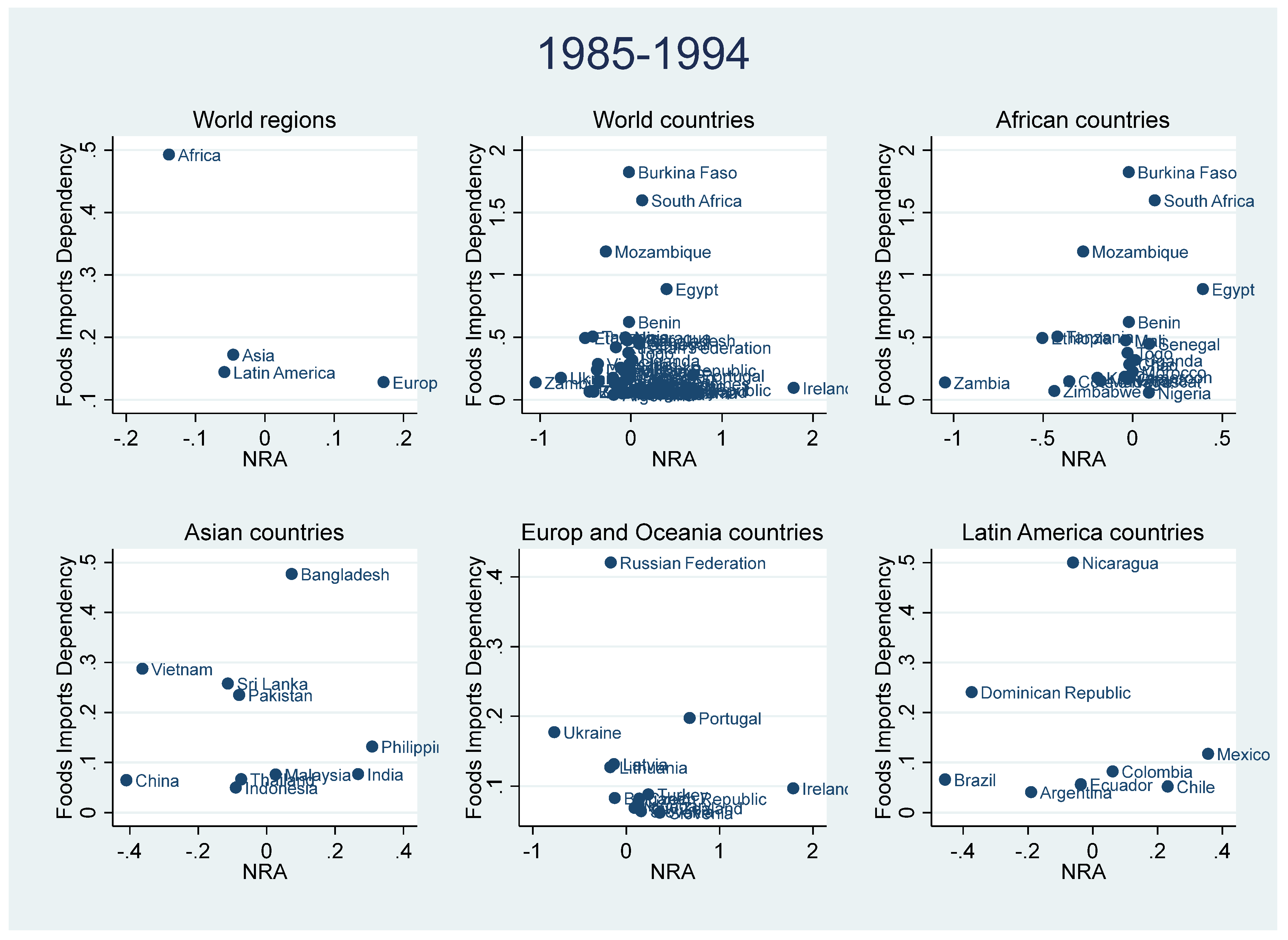
Figure A3.
Dose-response function and derivative. Source: Authors, 2021.
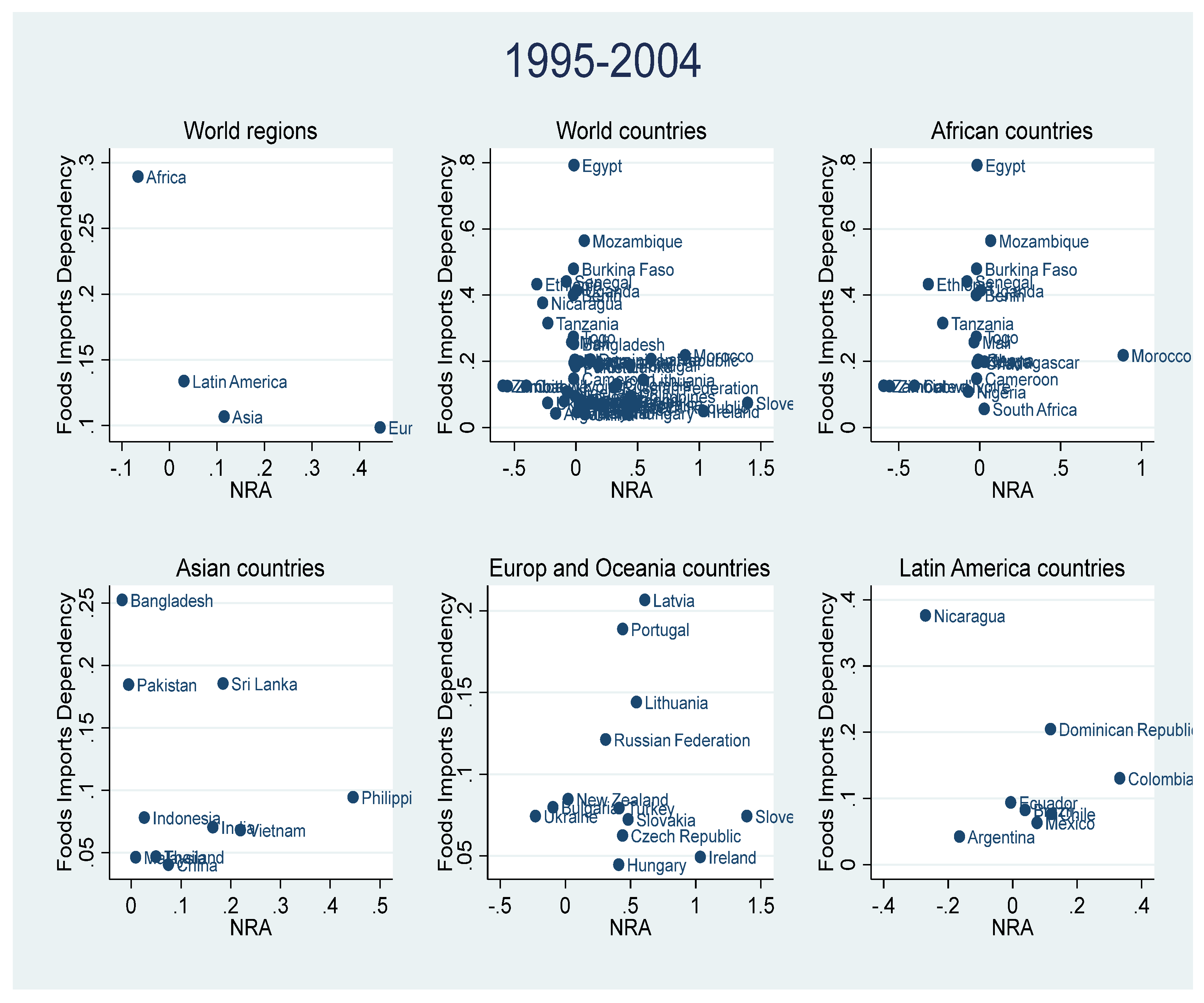
Figure A4.
Dose-response function and derivative. Source: Authors, 2021.
Appendix D
OLS Model Estimation
Table A1.
Dose-response model estimates with exogenous treatment.
| Dependent variable: lfidi | lfidi |
| t | -0.468*** |
| (-4.33) | |
| lcons | 2.692*** |
| (17.55) | |
| ltar | 0.310* |
| (2.54) | |
| lpop | 0.746*** |
| (4.30) | |
| lagripib | 0.164*** |
| (3.63) | |
| _ws_ltar | -0.088 |
| (-0.71) | |
| _ws_lpop | -0.926*** |
| (-5.33) | |
| _ws_lagripib | -0.185*** |
| (-4.05) | |
| Tw_1 | 0.0514 |
| (1.68) | |
| Tw_2 | -0.000 |
| (-1.58) | |
| Tw_3 | 0.000 |
| (1.35) | |
| cons | -3.542*** |
| (-9.36) | |
| R2 | 0.317 |
| N | 1716 |
Note: All the variables are specified in logarithms. T statistics. in parentheses *p < 0.05; **p < 0.01; ***p < 0.001. Source: Authors, 2021.
Looking at Figure A5, the derivative of the dose-response function reveals a convex parabola. The minimum of the derivative function is around the value 2, where the dose-response function has an inflection point.
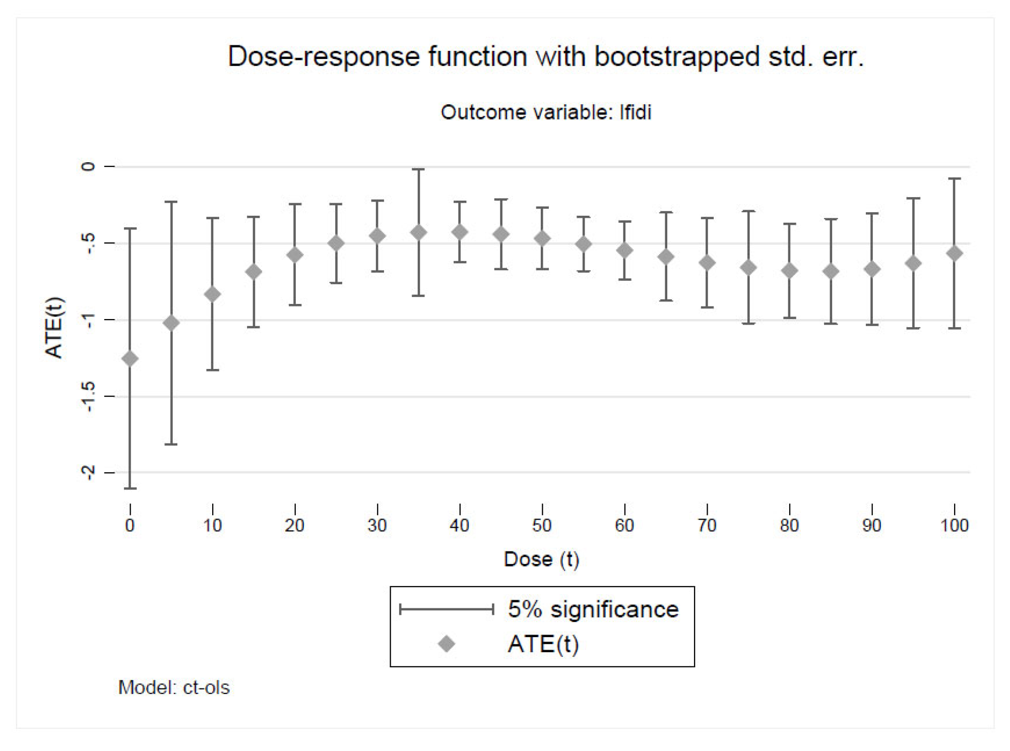
Figure A6 illustrates the results of dose-response function estimation with bootstrapped standard errors using 20 replications. The bootstrapped standard errors and the analytical standard errors show a similar pattern (see Figure A6).
Figure A5.
Dose-response function and derivative. Source : Authors, 2021.
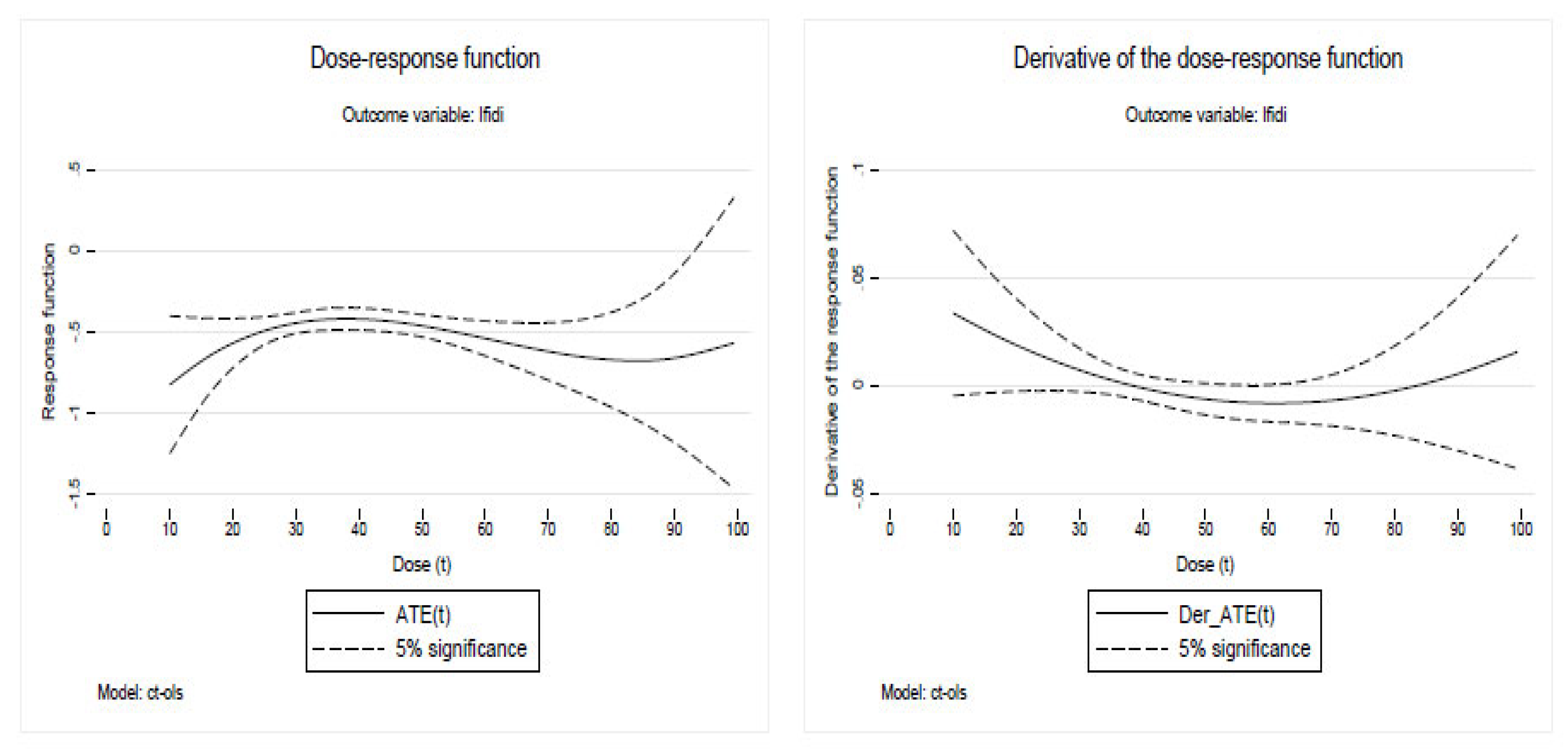
Figure A6.
Fonction dose-réponse avec bootstrapp sur l’erreur standard. Source : Authors, 2021.
Appendix E
Other Tables
Table A2.
Correlation table.
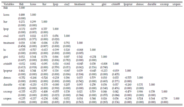 |
Source : Authors, 2021.
Table A3.
Heckman selection model.
| t | cna | |
| lcons | 4.506*** | -9.555*** |
| (0.62) | (3.02) | |
| ltar | -0.440*** | -0.637 |
| (0.13) | (0.487) | |
| lpop | 0.424*** | -0.166 |
| (0.13) | (0.32) | |
| lagripib | -0.039 | 0.322*** |
| (0.04) | (0.11) | |
| hc | 0.261*** | 1.213** |
| (0.18) | (0.58) | |
| gini | 0.039*** | -0.120*** |
| (0.01) | (0.03) | |
| crisis08 | -1.062*** | -1.189 |
| (0.26) | (1.67) | |
| lpoprur | 0.764*** | |
| (0.22) | ||
| democ | 0.232*** | |
| (0.06) | ||
| durable | 0.018*** | |
| (0.00) | ||
| xrcomp | -0.508** | |
| (0.20) | ||
| xropen | 0.024 | |
| (0.07) | ||
| _cons | -4.851*** | 50.888*** |
| (1.39) | (3.41) | |
| N | 1716 |
Note : All the variables are specified in logarithms. T statistics in parentheses *p < 0.05; **p < 0.01; ***p < 0.001. Source: Authors, 2021.
Table A4.
List of developing countries used in the study.
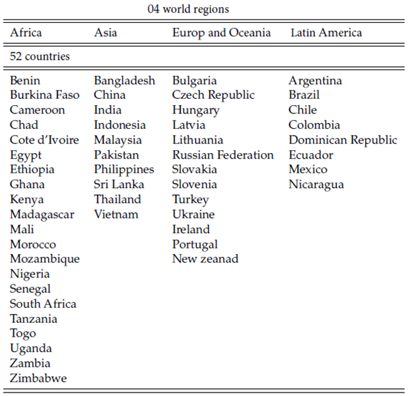 |
Source : Authors, 2021.
| 1 | See Appendix A. |
| 2 | See Appendix B. |
| 3 | A third-degree polynomial is used to allow for flexible non-linearities in the dose-response relationship, while avoiding overfitting that may arise with higher-order polynomials. This choice is consistent with prior applications in the continuous treatment literature (Cerulli [26]; Baum and Cerulli [18]). |
| 4 | To improve readability, detailed dose-response and derivative plots are reported in the Appendix. The main text focuses on the average treatment effects and their economic interpretation. |
| 5 | The kernel density estimate is a non-parametric estimate that allows the visualization of the distributions. |
| 6 | See the study regions in the Appendix E (Table 11) of this document. |
| 7 | The results of the t-test of the means reject at the 1% statistical threshold the equality of the observed means between the regions. |
References
- Abbott, P. C.; Morse, B. A. Tariff rate quota implementation and administration by developing countries. Agric. Resour. Econ. Rev. 2000, 29(1203-2016-95133), 115–124. [Google Scholar] [CrossRef]
- Acemoglu, D.; Johnson, S.; Robinson, J. A. The colonial origins of comparative development: An empirical investigation: Reply. Am. Econ. Rev. 2012, 102(6), 3077–3110. [Google Scholar] [CrossRef]
- Acemoglu, D.; Robinson, J. Economic backwardness in political perspective. Am. Polit. Sci. Rev. 2006, 100(1), 115–131. [Google Scholar] [CrossRef]
- Acemoglu, D.; Robinson, J. Political losers as a barrier to economic development. Am. Econ. Rev. Pap. Proc. 2000, 90, 126–130. [Google Scholar] [CrossRef]
- Anderson, K.; Strutt, A. Food security policy options for China: Lessons from other countries. Food Policy 2014, 49, 50–58. [Google Scholar] [CrossRef]
- Anderson, K. The political economy of agricultural price distortions; Cambridge Univer- sity Press, 2010. [Google Scholar]
- Anderson, K. Distortions to agricultural incentives: A global perspective; The World Bank, 2009. [Google Scholar]
- Anderson, K.; Hayami, Y.; Mulgan, A. G. The political economy of agricultural protection: East Asia in international perspective; World Scientific, 1986. [Google Scholar]
- Anderson, K.; Nelgen, S. Updated national and global estimates of distortions to agricultural incentives, 1955 to 2010. Database to be uploaded in March. 2012. [Google Scholar]
- Anderson, K.; Rausser, G.; Swinnen, J. Political economy of public policies: insights from distortions to agricultural and food markets. J. Econ. Lit. 2013, 51(2), 423–77. [Google Scholar] [CrossRef]
- Anderson, K.; Valenzuela, E. Global estimates of distortions to agricultural incen- tives, 1955 to 2007. 2008. Available online: www.
- Baliño, S.; Laborde, D.; Murphy, S.; Parent, M.; Smaller, C.; Traoré, F. Agricultural Bias in Focus; International Institute for Sustainable Development, 2019. [Google Scholar]
- Ballenger, N.; Mabbs-Zeno, C. Treating food security and food aid issues at the GATT. Food Policy 1992, 17(4), 264–276. [Google Scholar] [CrossRef]
- Basmann, R. L. On finite sample distributions of generalized classical linear identi- fiability test statistics. J. Am. Stat. Assoc. 1960, 55(292), 650–659. [Google Scholar] [CrossRef]
- Bastos, P.; Straume, O. R.; Urrego, J. A. Rain, agriculture, and tariffs. J. Int. Econ. 2013, 90(2), 364–377. [Google Scholar] [CrossRef]
- Bates, R. H.; Block, S. Political institutions and agricultural trade interventions in africa. Am. J. Agric. Econ. 2011, 93(2), 317–323. [Google Scholar] [CrossRef]
- Baum, C. F.; Cerulli, G. Estimating a dose-response function with heterogeneous response to confounders when treatment is continuous and endogenous. Working Paper 9388, 2016; EcoMod. [Google Scholar]
- Bawn, K.; Rosenbluth, F. Coalition parties versus coalititions of parties. How electoral agency shapes the political logic of costs and benefits. Am. J. Polit. Sci. 2006, 50(2), 251–266. [Google Scholar] [CrossRef]
- Becker, H. S. Mondes de l’art et types sociaux. Sociol. Du. Trav. 1983, 404–417. [Google Scholar] [CrossRef]
- Besley, T.; Persson, T.; Sturm, D.M. Political competition, policy, and growth: Theory and evidence from the United States. Rev. Econ.Stud. 2010, 77(4), 1329–1352. [Google Scholar] [CrossRef]
- Bia, M.; Mattei, A. A stata package for the estimation of the dose-response function through adjustment for the generalized propensity score. Stata J. 2008, 8(3), 354–373. [Google Scholar] [CrossRef]
- Burgess, R.; Donaldson, D. Can openness mitigate the effects of weather shocks? Evidence from India’s famine era. Am. Econ. Rev. 2010, 100(2), 449–453. [Google Scholar] [CrossRef]
- Bushway, S.; Johnson, B.D.; Slocum, L.A. La magie est-elle toujours là ? L’utilisation de la correction en deux étapes de Heckman pour le biais de sélection en criminologie. J. De Criminol. Quant. 2007, 23(2), 151–178. [Google Scholar] [CrossRef]
- Butault, J.-P.; Le Mouël, Chantai. « Pourquoi et comment intervenir en agriculture? » dans. In Les Soutiens à l’agriculture, théorie, histoire, mesure; INRA Éditions: Paris, 2004; pp. 11–67. [Google Scholar]
- Campbell, D. J. Strategies for coping with severe food deficits in rural Africa: a review of the literature. Food Foodways 1990, 4(2), 143–162. [Google Scholar] [CrossRef]
- Cerulli, G. ctreatreg: Command for fitting dose–response models under exogenous and endogenous treatment. Stata J. 2015, 15(4), 1019–1045. [Google Scholar] [CrossRef]
- Cerulli, G.; et al. A continuous treatment model for estimating a dose response func- tion under endogeneity and heterogeneous response to observable confounders: Descrip- tion and implementation via the stata module “ctreatreg”; Technical report; Institute for Economic Research on Firms and Growth-Moncalieri (TO) ITALY., 2012. [Google Scholar]
- Croser, J.; Anderson, K. Changing contributions of different agricultural policy instruments to global reductions in trade and welfare. World Trade Rev. 2011, 10(3), 297–323. [Google Scholar] [CrossRef]
- De Grauwe, P. Exchange rate variability and the slowdown in growth of international trade. Staff Pap. 1988, 35(1), 63–84. [Google Scholar] [CrossRef] [PubMed]
- De Schutter, O. Acquisitions et locations de terre à grande échelle: ensemble de principes minimaux et de mesures pour relever le défi au regard des droits de l’homme; Assemblée Générale des Nations Unies, 2009. [Google Scholar]
- Díaz-Bonilla, E.; Ron, J. F. Food security, price volatility, and trade: Some reflec- tions for developing countries. Issue paper, 2010; 8. [Google Scholar]
- Downs, A. An Economic Theory of Democracy; Harper Collins: New York, 1957. [Google Scholar]
- Durbin, J. Errors in variables. In Revue de l’institut International de Statistique; 1954; pp. pages 23–32. [Google Scholar]
- Fałkowski, J.; Olper, A. Political competition and policy choices: the evidence from agricultural protection. Agric. Econ. 2014, 45(2), 143–158. [Google Scholar] [CrossRef]
- Feenstra, Robert C.; Inklaar, Robert; Timmer, Marcel P. Human capital in PWT 9.0. In Groningen Growth and Development Centre, University of Groningen; 2015. [Google Scholar]
- Finger, R.; El Benni, N. A note on the effects of the Income Stabilization Tool on income inequality in agriculture. J. Agric. Econ. 2014, 65(3), 739–745. [Google Scholar] [CrossRef]
- Flatters, F. Measuring the impacts of trade policies: Effective rates of protection; Technical report; Citeseer, 2005. [Google Scholar]
- Fuglie, K. R&D capital, R&D spillovers, and productivity growth in world agriculture. Appl. Econ. Perspect. Policy 2018, 40(3), 421–444. [Google Scholar]
- Gawande, K.; Hoekman, B. Lobbying and agricultural trade policy in the united states. Int. Organ. 2006, 60(3), 527–561. [Google Scholar] [CrossRef]
- Grant, J. H.; Boys, K. A. Agricultural trade and the GATT/WTO: Do membership make a difference? Am. J. Agric. Econ. 2012, 94(1), 1–24. [Google Scholar] [CrossRef]
- Guardabascio, B.; Ventura, M. Estimating the dose–response function through a generalized linear model approach. Stata J. 2014, 14(1), 141–158. [Google Scholar] [CrossRef]
- Gwartney, J. D.; Lawson, R.; Holcombe, R. G. The size and functions of government and economic growth; Joint Economic Committee: Washington, 1998; pp. 1–32. [Google Scholar]
- Hammoudi, A.; Hamza, O.; Migliore, S. Sécurité alimentaire dans les pays en développement: quelle contribution des Filières d’exportation? Rev. D’économie Polit. 2015, 125(4), 601–631. [Google Scholar] [CrossRef]
- Hassan, R.; Greenaway, D.; Reed, G. V. Nominal and effective protection in the Egyptian agricultural sector: a multicommodity analysis. Appl. Econ. 1992, 24(5), 483–492. [Google Scholar] [CrossRef]
- Hausman, J. A. Specification tests in econometrics. Econom. J. Econo-Metr. Soc. 1978, pages 1251–1271. [Google Scholar] [CrossRef]
- Hausman, J. A. An instrumental variable approach to full information estimators for linear and certain nonlinear econometric models. Econom. J. Econom. Soc. 1975, 727–738. [Google Scholar] [CrossRef]
- Heckman, J. J. Sample selection bias as a specification error. Econom. J. Econom. Soc. 1979, pages 153–161. [Google Scholar] [CrossRef]
- Heslop, A. Redistricting: The Key to Politics in the 1980’s; Rose Institute of State and Local government, 1980. [Google Scholar]
- Hirano, K.; Imbens, G. W. The propensity score with continuous treatments. Appl. Bayesian Model. Causal Inference From Incomplete-Data Perspect. 2004, 226164, 73–84. [Google Scholar]
- Jayne, T. S.; Rashid, S. Input subsidy programs in sub-Saharan Africa: a synthesis of recent evidence. Agric. Econ. 2013, 44(6), 547–562. [Google Scholar] [CrossRef]
- Josling, T.; Valdés, A. Agricultural policy indicators. Technical report. 2004. [Google Scholar]
- Lamb, R. L. Food crops, exports, and the short-run policy response of agriculture in Africa. Agric. Econ. 2000, 22(3), 271–298. [Google Scholar] [CrossRef]
- Larochez-Dupraz, C.; Huchet-Bourdon, M. Agricultural support and vulnerabi- lity of food security to trade in developing countries. Food Secur. 2016, 8(6), 1191–1206. [Google Scholar] [CrossRef]
- Magrini, E.; Montalbano, P.; Nenci, S.; Salvatici, L. Agricultural (dis) incentives and food security: Is there a link? Am. J. Agric. Econ. 2017, 99(4), 847–871. [Google Scholar] [CrossRef]
- Marchenko, Y. V.; Genton, M. G. A heckman selection-t model. J. Am. Stat. Assoc. 2012, 107(497), 304–317. [Google Scholar] [CrossRef]
- Medellín-Azuara, J.; Howitt, R. E.; Harou, J. J. Predicting farmer responses to water pricing, rationing and subsidies assuming profit maximizing investment in irrigation technology. Agric. Water Manag. 2012, 108, 73–82. [Google Scholar] [CrossRef]
- Morin-Rivet, L. Le découplage des aides aux revenus: un concept économique imprécis; 2008. [Google Scholar]
- Olper, A. Determinants of agricultural protection: The role of democracy and institutional setting Alessandro Olper. J. Agric. Econ. 2001, 52(2), 75–92. [Google Scholar] [CrossRef]
- Olper, A.; Raimondi, V. Electoral rules, forms of government and redistributive policy: Evidence from agriculture and food policies. J. Comp. Econ. 2013, 41(1), 141–158. [Google Scholar] [CrossRef]
- Olper, A.; Raimondi, V. Constitutional rules and agricultural policy outcomes; World Bank, 2009. [Google Scholar]
- Olson, M. Agricultural exploitation and subsidization: There is an explanation. Choices 1990, 5, 316-2016-7378. [Google Scholar]
- OECD. Agriculture in a changing world: which policies for tomorrow? Press communiqué SG/COM? NEWS? (98)22; OECD: Paris, 1998. [Google Scholar]
- Persson, T.; Roland, G.; Tabellini, G. Separation of powers and political accountability. Quart. J. Econ. 1997, 112(4), 1163–1202. [Google Scholar] [CrossRef]
- Peterman, A.; Behrman, J. A.; Quisumbing, A. R. A review of empirical evidence on gender differences in nonland agricultural inputs, technology, and services in developing countries. Gend. Agric. 2014, 145–186. [Google Scholar]
- Rubin, D. B. Causal inference using potential outcomes: Design, modeling, decisions. J. Am. Stat. Assoc. 2005, 100(469), 322–331. [Google Scholar] [CrossRef]
- Santos-Paulino, A. U. The effects of trade liberalization on imports in selected developing countries. World Dev. 2002, 30(6), 959–974. [Google Scholar] [CrossRef]
- Sargan, J. D. The estimation of economic relationships using instrumental variables; Journal of the Econometric Society: Econometrica, 1958; pp. pages 393–415. [Google Scholar]
- Sen, A. Food and freedom; Washington, DC-October, 1987; volume 29. [Google Scholar]
- Sheikhi, A.; Bahador, F.; Arashi, M. On a generalization of the test of endogeneity in a two stage least squares estimation. In Journal of Applied Statistics; 2020; pp. pages 1–13. [Google Scholar]
- Swinnen, J. F. A positive theory of agricultural protection. Am. J. Agri-Cult. Econ. 1994, 76(1), 1–14. [Google Scholar] [CrossRef]
- Swinnen, J.; de Gorter, H.; Rausser, G.C.; Banejee, A. N. The Political Economy of Public Research Investment and Commody Policy in Agriculture: An Empirical Study. Agn’mkural Econ. 2000a, 22, 11 1–122. [Google Scholar]
- Swinnen, J. F. Political economy of agricultural distortions: The literature to date; World Bank, 2009. [Google Scholar]
- Tello, M. D. Non tariffs barriers’ rates of nominal protection faced by developing countries’ exporters of agricultural products: The case of Peru, 2000-2008. Glob. Horiz. 2008, 2(1), 27–56. [Google Scholar]
- Thies, C. G.; Porche, S. The political economy of agricultural protection. J. Politics 2007, 69(1), 116–127. [Google Scholar] [CrossRef]
- Thomson, H. Food and power: agricultural policy under democracy and dictatorship. Comp. Politics 2017, 49(2), 273–296. [Google Scholar] [CrossRef]
- Thomson, H. Food and power: Regime type, agricultural policy, and political stability; Cambridge University Press, 2019. [Google Scholar]
- Weersink, A. The growing heterogeneity in the farm sector and its implications. Can. J. Agric. Econ. Can. D’agroeconomie 2018, Vol. 66(No. 1), 27–41. [Google Scholar] [CrossRef]
- Wolfe, R. Yours is bigger than mine! Could an index like the Producer Subsidy Equivalent help in understanding the comparative incidence of industrial subsidies? World Econ. 2021, 44(2), 328–345. [Google Scholar] [CrossRef]
- World Bank. Reforming Trade, Price, and Subsidy Policies; 2007. [Google Scholar]
- Wu, D.-M. Alternative tests of independence between stochastic regressors and disturbances; journal of the Econometric Society: Econometrica, 1973; pp. pages 733–750. [Google Scholar]
Figure 1.
Dose-response function and derivative. Source : Authors’ calculations based on World Bank and FAO data.
Figure 1.
Dose-response function and derivative. Source : Authors’ calculations based on World Bank and FAO data.
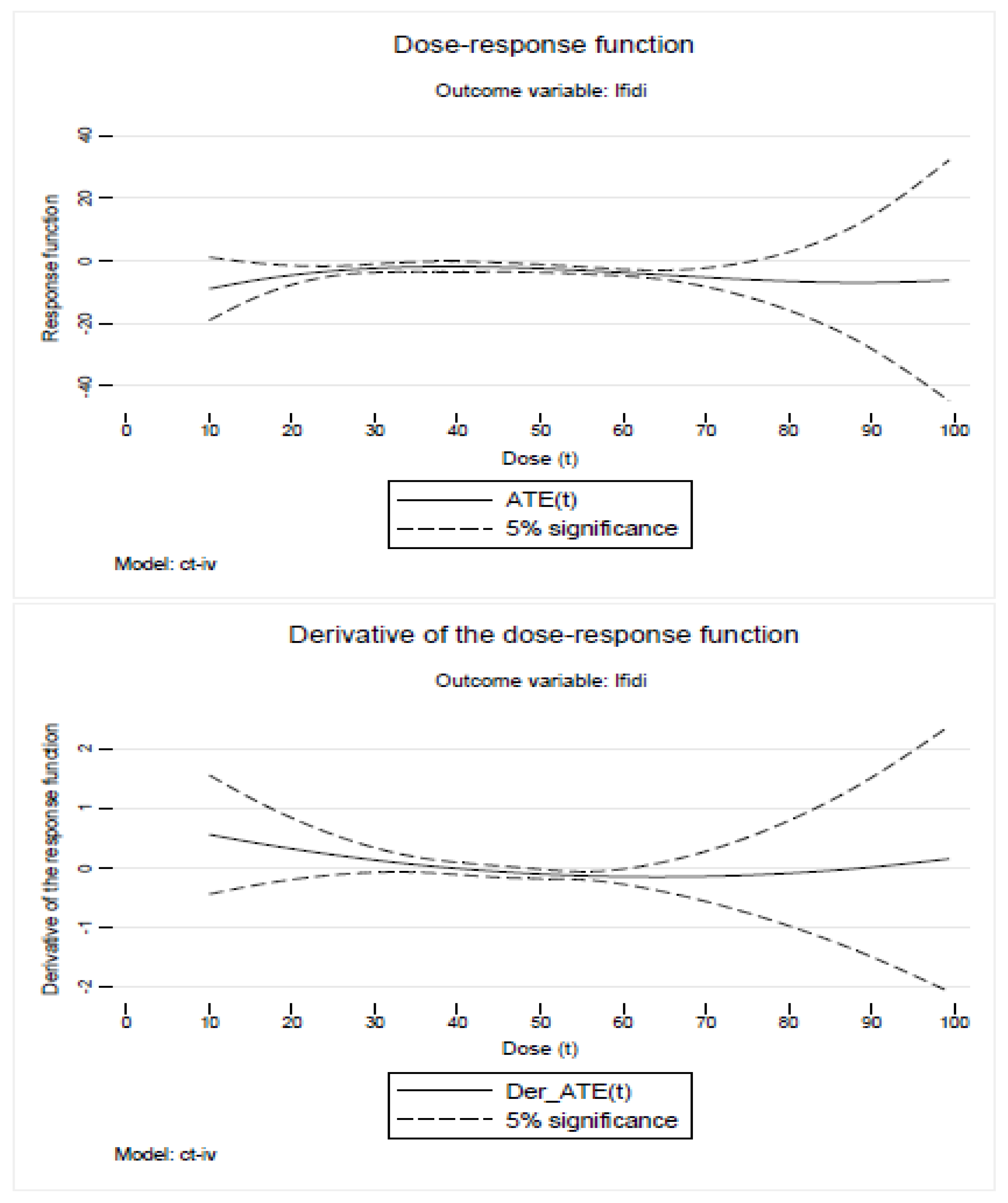
Figure 2.
Distribution of treatment effects and dose-response function. Source: Authors’ calculations based on World Bank and FAO data.
Figure 2.
Distribution of treatment effects and dose-response function. Source: Authors’ calculations based on World Bank and FAO data.
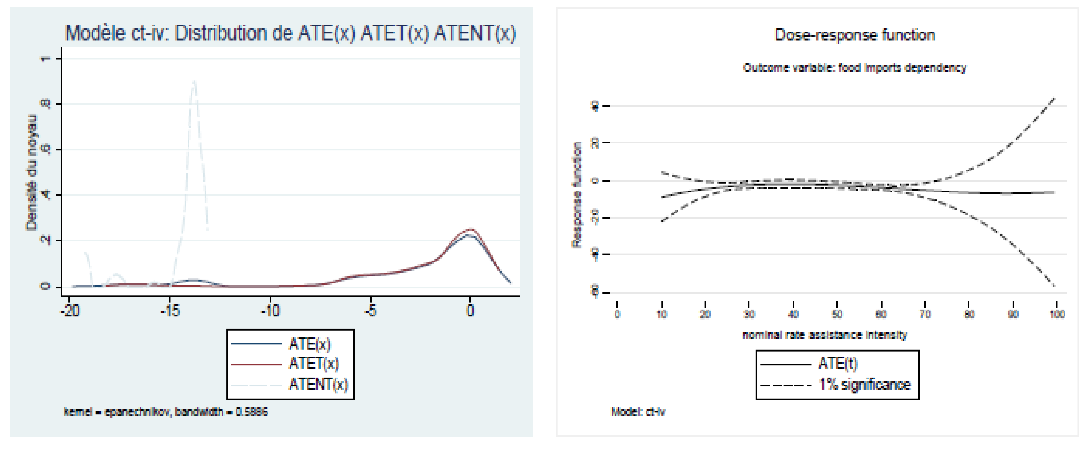
Table 1.
Variables.
| Variables | Meanings and references | Sources | |
| Dependent variable | |||
| lfidi | logarithm of the food import dependency index (in %) (Larochez-Dupraz et al., 2016) | The method of calculation and the sources of the data used are specified in the following paragraphs. |
|
| Treatment variables | |||
| cna | nominal assistance coefficient (Magrini et al., 2017) | Calculated from nominal rate data. These are taken from the World Bank database (see details in the following paragraphs). | |
| t | binary variable that takes the value 1 if cna>0 and 0 if cna=0 (Magrini et al., 2017) | Calculations of authors | |
| Covariates | |||
| lcons | logarithm of the annual growth rate of household consumption expenditure per capita (in %) (Swinnen, 2009; Thies and Porche, 2007) | World Bank (Https ://data.worldbank.org/indicator/ //NE.CON.PRVT.PC.KD. ZG) |
|
| ltar | logarithm of average tariff rates applied (in %) (Magrini et al., 2017) | World Bank (Https ://data.worldbank.org/indicator/ //TM.TAX.MRCH.WM.AR.ZS) |
|
| lpop | logarithm of total population (in 100 million people) (Magrini et al. 2017) | World Bank (Https ://data.worldbank.org/indicator/ //SP.POP.TOTL) |
|
| lagri | logarithm of share of agricultural production in GDP (in %) (Magrini et al. 2017) | World Bank (Https ://data.worldbank.org/indicator/ //SP.POP.TOTL) |
|
| Instruments | |||
| cna | hc | human capital index (in %) (Feenstra and al., 2015) | Growth and Development Centre of Groningen (www.ggdc.net/pwt) |
| gini | gini index (Swinnen, 1994) | World Bank (http ://ire- search.worldbank.org/PovcalNet/index.htm) |
|
| t | democ | democracy index (Olper et Raimondi, 2013) | Center for systemic peace (https ://www.systemicpeace.org/inscrdata.html) |
| durable | indicator of the sustainability of schemes (Olper et Raimondi, 2013) | Center for systemic peace (https ://www.systemicpeace.org/inscrdata.html) |
|
| xropen | opening indicator for executive recruitment (Fałkowskia and Olper, 2013) | Center for systemic peace (https ://www.systemicpeace.org/inscrdata.html) |
|
| xrcomp | competitiveness indicator for executive recruitment (Fałkowskia and Olper, 2013) | Center for systemic peace (https ://www.systemicpeace.org/inscrdata.html) |
|
| hc | human capital index (en %) (Feenstra et al., 2015) | Growth and Development Centre of Groningen (www.ggdc.net/pwt) | |
| gini | gini index (Swinnen, 1994) | World bank (http ://ire- search.worldbank.org/PovcalNet/index.htm) |
|
Source: Authors.
Table 2.
Descriptive statistics.
| Variable | Description (units) | Mean | Std. Dev. | Min | Max |
| fidi | food import dependency ratio (in %) | 0.2108 | 0.2864 | 0.1328 | 4.9876 |
| cons | growth rate of per capita consumption expenditure (in %) | 0.6542 | 0.1281 | 0.2748 | 1.3842 |
| tar | average of the weighted tariff rates per imported product (in %) |
9.6665 | 7.4791 | 0.0440 | 56.3600 |
| pop | total population (in millions of inhabitants) | 85.1634 | 226.5825 | 1.9434 | 1421.0220 |
| cna | nominal assistance coefficient | 38.8640 | 12.0160 | 0 | 100 |
| t | binary variable which takes the value 1 if cna> 0 and 0 if cna = 0 | 0.9435 | 0.2310 | 0 | 1 |
| hc | human capital index | 2.1810 | 0.6620 | 1.0220 | 3.7940 |
| gini | gini index | 41.0970 | 9.1680 | 19.1720 | 64.80 |
| agripib | production of the agricultural sector (in % of GDP) | 0.2975 | 2.1740 | 4.92×10⁻⁶ | 57.0475 |
| poprur | rural population (in millions of inhabitants) | 48.8789 | 147.0594 | 0.5185 | 889.2167 |
| democ | democracy index | 5.2930 | 3.6750 | 0 | 10 |
| durable | sustainability index of regimes | 18.5820 | 22.8380 | 0 | 140 |
| xrcomp | competitiveness index for executive recruitment | 2.0520 | 1.0840 | 0 | 3 |
| xropen | opening index of executive recruitment | 3.4580 | 1.3410 | 0 | 4 |
| N | sample size | 1716 |
Source : Authors.
Table 4.
Dose-response model estimates with endogenous treatment.
| Dependent variable | lfidi |
| t | -2.827*** |
| (-2.09) | |
| _ws_ltar | 0.679 |
| (1.23) | |
| _ws_lpop | -3.436*** |
| (-5.22) | |
| _ws_lagripib | -1.833*** |
| (-4.90) | |
| Tw_1 | 0.845 |
| (1.01) | |
| Tw_2 | -0.0156 |
| (-0.83) | |
| Tw_3 | 0.000 |
| (0.60) | |
| lcons | 2.501*** |
| (7.48) | |
| ltar | -0.413 |
| (-0.80) | |
| lpop | 3.229*** |
| (5.04) | |
| lagripib | 1.87*** |
| (4.71) | |
| _cons | 1.290 |
| (0.77) | |
| N | 1716 |
Note : All the variables are specified in logarithms.T statistics in parentheses *p < 0.05; **p < 0.01; ***p < 0.001. Source: Authors’ calculations based on World Bank and FAO data.
Table 5.
Statistics on average treatment effects.
| Variables | Mean | N |
| ATE | -2.827 | 1716 |
| ATET | -2.136 | 1619 |
| ATENT | -14.363 | 97 |
Source: Authors’ calculations based on World Bank and FAO data.
Table 6.
Average effect statistics by region.
| Variable | Statistics | Africa | Asia | Europ and Oceania | Latin America |
| ATE(x) | Mean | -1,201 | -6,200 | -3,411 | -1,933 |
| Std. Dev. | 0,12 | 0,31 | 0,23 | 0,18 | |
| N | 693 | 330 | 429 | 264 | |
| ATET(x) | Mean | -0,644 | -6,028 | -1,724 | -1,664 |
| Std. Dev. | 0,06 | 0,31 | 0,09 | 0,15 | |
| N | 663 | 325 | 373 | 258 | |
| ATENT(x) | Mean | -13,518 | -17,315 | -14,645 | -13,489 |
| Std. Dev. | 0,06 | 0,4 | 0,24 | 0,01 | |
| N | 30 | 5 | 56 | 6 |
Source : Authors’ calculations based on World Bank and FAO data.
Table 7.
Descriptive statistics of covariates in the analysis of treatment effects by region.
| Variable | Statistics | Africa | Asia | Europ and Oceania | Latin America |
| nra | Moyenne | -0,067 | 0,042 | 0,263 | 0,001 |
| Ecart-type | 0,28 | 0,26 | 0,48 | 0,28 | |
| cons | Moyenne | 0,728 | 0,618 | 0,554 | 0,669 |
| Ecart-type | 0,12 | 0,12 | 0,08 | 0,08 | |
| tar | Moyenne | 11,549 | 13,971 | 3,763 | 8,938 |
| Ecart-type | 6,16 | 10,78 | 2,47 | 4,44 | |
| pop | Moyenne | 28930,490 | 310754,300 | 24537,780 | 49301,250 |
| Ecart-type | 30488,27 | 444426,50 | 39840,18 | 56537,12 | |
| agri_pib | Moyenne | 0,406 | 0,006 | 0,473 | 0,084 |
| Ecart-type | 3,22 | 0,01 | 1,42 | 0,38 | |
| hc | Moyenne | 1,653 | 2,151 | 2,946 | 2,362 |
| Ecart-type | 0,40 | 0,44 | 0,45 | 0,37 | |
| gini | Moyenne | 42,805 | 37,746 | 34,057 | 52,239 |
| Ecart-type | 7,61 | 6,28 | 7,61 | 5,00 | |
| poprur | Moyenne | 66,075 | 64,544 | 33,935 | 27,129 |
| Ecart-type | 12,57 | 13,37 | 9,27 | 12,22 | |
| democ | Moyenne | 2,887 | 4,594 | 8,520 | 7,239 |
| Ecart-type | 3,05 | 3,49 | 2,17 | 2,03 | |
| xrcomp | Moyenne | 12,266 | 23,882 | 26,065 | 16,375 |
| Ecart-type | 12,90 | 20,94 | 35,03 | 13,48 | |
| xropen | Moyenne | 1,355 | 2,109 | 2,739 | 2,693 |
| Ecart-type | 1,06 | 1,02 | 0,52 | 0,70 | |
| durable | Moyenne | 2,860 | 3,721 | 3,972 | 3,865 |
| Ecart-type | 1,75 | 1,02 | 0,33 | 0,73 | |
| N | 693 | 330 | 429 | 264 | |
Source : Authors’ calculations based on World Bank and FAO data.
Disclaimer/Publisher’s Note: The statements, opinions and data contained in all publications are solely those of the individual author(s) and contributor(s) and not of MDPI and/or the editor(s). MDPI and/or the editor(s) disclaim responsibility for any injury to people or property resulting from any ideas, methods, instructions or products referred to in the content. |
© 2026 by the authors. Licensee MDPI, Basel, Switzerland. This article is an open access article distributed under the terms and conditions of the Creative Commons Attribution (CC BY) license (http://creativecommons.org/licenses/by/4.0/).
Copyright: This open access article is published under a Creative Commons CC BY 4.0 license, which permit the free download, distribution, and reuse, provided that the author and preprint are cited in any reuse.


