

Submitted:
23 April 2026
Posted:
08 May 2026
You are already at the latest version
Preprints on COVID-19 and SARS-CoV-2
Abstract
A three-year (January 2020–December 2022) daily dataset of 16 polycyclic aromatic hydrocarbons (PAHs) co-sampled with PM2.5 and a suite of meteorological variables at a Mediterranean coastal urban site in southern Italy (Pomigliano d’Arco, Campania) is presented and analysed. Raw PAH time series were decomposed into a long-term trend component (LT), a seasonal component (ST), and a residual component (RT) using an iterative missing-value-robust Kolmogorov–Zurbenko (KZ) moving-average filter. Spearman rank correlations between PAH concentrations and four meteorological predictors (mean temperature, relative humidity, mean wind speed, and maximum wind speed) were computed for each congener. Diagnostic molecular ratios — Fluoranthene/(Fluoranthene+Pyrene), BaP/BghiP, Indeno[1,2,3-cd]pyrene/(IcdP+BghiP), and Benz[a]anthracene/(BaA+Chrysene) — were evaluated seasonally and subjected to an information-theoretic Bayesian mixture modelling procedure (SNOB/MML) to estimate the number and nature of prevailing emission source classes. Total PAH concentrations (sum of 16 congeners) ranged from <1 ng m−3 in summer to 46 ng m−3 during winter high-pollution episodes, with BaP peaking at ≈6.7 ng m−3. Pronounced seasonal variability was driven primarily by residential heating emissions, and the incremental lifetime cancer risk (ILCR) for inhalation exposure reached 1.03×10⁻⁴ (95% CI: 0.88−1.20×10⁻⁴) during the heating season, exceeding standard regulatory thresholds. An anomalous near-background PAH signal during spring 2020 is attributed to the COVID-19 national lockdown, which reduced total PAH concentrations by approximately 85% relative to the seasonal component predicted by the iterative moving-average filter for the same calendar window. Source apportionment via diagnostic ratios identifies residential/biomass combustion as the dominant cold-season source and vehicular emissions as the prevailing warm-season source. These results provide a novel characterisation of PAH pollution dynamics in the undersampled southern Mediterranean and offer insights for targeted abatement policies.
Keywords:
polycyclic aromatic hydrocarbons
; PM2.5
; Mediterranean air quality
; source apportionment
; time-series decomposition
; Bayesian mixture model
; benzo[a]pyrene
; seasonal variability
; COVID-19 lockdown
; Italy
1. Introduction
Polycyclic aromatic hydrocarbons (PAHs) are persistent organic pollutants generated predominantly through the incomplete combustion of organic matter [1]. Their chemical structure — two or more fused aromatic rings — determines both their physical behaviour and their toxicological relevance: high-molecular-weight (HMW, 4–6 rings) species partition preferentially onto the PM2.5 fraction and can thus penetrate deeply into the human respiratory tract [2]. Benzo[a]pyrene (BaP), the most widely studied congener, is classified as a Group 1 human carcinogen by the International Agency for Research on Cancer (IARC) [3]. European Directive 2004/107/EC establishes an annual target value of 1 ng m−3 for BaP measured in the PM10 fraction [4]. Despite this framework, approximately 31% of European monitoring stations recorded exceedances in 2016 [5], highlighting persistent gaps between policy ambition and ambient reality.
Atmospheric PAH concentrations in urban environments have been documented to exceed those in rural areas by approximately one order of magnitude, with vehicle exhaust and industrial emissions identified as the primary anthropogenic sources in the majority of studies conducted worldwide [6]. Despite this broad consensus, high-temporal-resolution monitoring records for the southern Mediterranean basin remain comparatively scarce, limiting the ability to quantify source contributions and assess population exposure with confidence in this atmospherically distinct region [7].
In urban environments, PAH concentrations are far from static: they fluctuate over hours, seasons, and years in response to emission patterns and atmospheric conditions. Seasonal contrasts are particularly striking in southern Europe, where winter concentrations can exceed summer values by one to two orders of magnitude. This contrast arises from the combined effect of increased residential heating emissions during cold months, a shallower boundary layer that limits atmospheric dilution, and the much stronger photochemical degradation characteristic of Mediterranean summers. The Mediterranean basin represents a distinct atmospheric setting — warm, dry summers alternate with mild, wet winters and a heterogeneous mix of emission sources including vehicular traffic, shipping, industrial facilities, and domestic combustion [7]. Against this background, a multi-year dataset collected at a single well-characterised site is particularly valuable, as it disentangles the inter-annual consistency of source patterns from episodic variability driven by short-term meteorological forcing.
Road traffic constitutes one of the principal sources of PM-bound PAHs in urban areas, emitting both primary particles and gaseous precursors. A tunnel experiment carried out in the Campania region quantified real-world PAH emission factors and concentration profiles from the local vehicle fleet [8]. Complementary measurements of inorganic ionic species in the same tunnel campaign showed that road traffic accounts for approximately 10% of PM mass as water-soluble ions, underlining the chemical complexity of traffic-related aerosol [9]. At broader spatial scales, PM2.5 and PM10 chemical composition in the Naples metropolitan area has been further characterised in terms of ionic balance, metal concentrations, and air-mass back-trajectory clusters [10], providing essential contextual information for In addition, ship-related exhaust has been characterised through direct stack sampling on high-speed passenger vessels in the Gulf of Naples, providing detailed chemical fingerprints for PM10 emitted by marine traffic [11].
Beyond purely observational studies, data assimilation frameworks that fuse ground-based measurements with chemical transport model (CTM) ensembles have been shown to provide spatially and temporally resolved diagnostics of particulate pollution over large domains. For example, Chianese et al. [12] implemented a Bayesian hierarchical data-assimilation approach that combines daily PM10 observations from the Italian monitoring network with CAMS ensemble forecasts over the Po Valley, achieving a substantial reduction of model bias and an out-of-sample of 0.83. Their results underscore the added value of integrating observational and modelling information when assessing population exposure, particularly in regions where monitoring stations are sparsely distributed.
Molecular diagnostic ratios have long served as practical tools for identifying PAH emission sources, exploiting the fact that the relative abundance of isomeric congeners differs systematically between pyrogenic and petrogenic sources [13]. Ratios such as Fla/(Fla+Pyr), BaP/BghiP, IcdP/(IcdP+BghiP), and BaA/(BaA+Chr) carry source-specific information, yet their interpretation is complicated by atmospheric ageing, phase repartitioning, the mixing of multiple source types, and measurement uncertainties near detection limits [14]. Probabilistic and information-theoretic clustering of ratio vectors offers a more principled alternative to simple threshold-based decision trees. Earlier work on PAH contamination in rural Campanian soils already demonstrated the diagnostic power of these ratios and their limitations when sources overlap [15], providing a regional baseline against which atmospheric PAH levels can be contextualised.
The COVID-19 pandemic provided an exceptional natural experiment for air-quality research: the Italian national lockdown (9 March – 4 May 2020) sharply reduced traffic, industrial output, and commercial activity, creating a unique opportunity to isolate anthropogenic PAH contributions from baseline background levels [16,17]. Quantifying the resulting reduction in PM2.5 is of direct relevance for impact assessment, since uncertainties in modelled PM2.5 fields propagate substantially into estimates of premature mortality and crop damage [18]; an observational dataset with near-zero anthropogenic influence therefore provides a valuable reference for reducing such uncertainties.
The present study brings together these threads by (i) presenting and analysing a three-year daily PAH time series at a southern Italian Mediterranean urban site (Pomigliano d’Arco, Campania); (ii) decomposing PAH signals into long-term trend, seasonal, and residual components via an iterative missing-value-robust moving-average filter; (iii) quantifying Spearman rank correlations between each congener and key meteorological variables; (iv) applying diagnostic ratio analysis combined with a Bayesian minimum message length mixture model to characterise emission source classes; (v) estimating incremental lifetime cancer risk through toxic equivalency factors and Monte Carlo uncertainty propagation; and (vi) documenting the PAH response to the COVID-19 lockdown. Together, these analyses yield an original, multidimensional picture of PM2.5-bound PAH dynamics in a region that is atmospherically significant yet chronically undermonitored.
2. Materials and Methods
2.1. Monitoring Site and Sampling
Sampling was conducted from January 2020 to December 2022, covering three complete annual cycles, in the city of Pomigliano d’Arco, Italy (40.908∘ N, 14.392∘ E), on the roof of the Town Hall (Figure 1). Pomigliano d’Arco is located approximately 15 km north-east of Naples city centre and is part of the wider Naples metropolitan area. The city hosts one of the largest industrial districts in southern Italy, situated within the municipal territories of Acerra and Pomigliano d’Arco, bordering the municipality of Castello di Cisterna. The monitoring site combines residential zones, major road arteries, and more distant industrial areas, making it well suited for source apportionment studies that aim to disentangle combustion from traffic and industrial contributions. Sampling was conducted using a SWAM 5a Dual Channel Monitor low-volume sequential sampler (FAI Instruments s.r.l., Rome, Italy), set at a volumetric flow rate of 2.3 m3/h. Although the SWAM 5a instrument collects PM10 and PM2.5 fractions concurrently, only the PM2.5 fraction was subjected to PAH analysis in this study, consistent with the primary research objective of characterising fine-particle-bound PAH dynamics. As required by the UNI-EN 12341:2014 standard, each sampling period lasted 24 h and the sample was collected on quartz filters (Whatman, 47 mm diameter, 0.45 m pore size). After collection, filters were stored at 4∘ C until analysis. A total of 872 valid samples were collected over the three years, corresponding to 79% of possible sampling days, well above the 33% minimum required by the EU Commission directive for calculating yearly average BaP concentrations.
2.2. Analytical Methods
Particulate-phase PAH material was analysed for 16 priority congeners following the ISO 12884 protocol using Gas Chromatography–Mass Spectrometry (GC-MS; TQ8030, Shimadzu) in selected ion monitoring mode. Chemical analysis was performed on PM2.5 samples following the procedure described in Annex VI of Italian Legislative Decree 155/2010. Compound determination was carried out after ultrasonic extraction, extending the official UNI-EN 15549:2008 method (originally validated for BaP alone) to the other 15 congeners: naphthalene (Nap), acenaphthylene (Acy), acenaphthene (Ace), fluorene (Flu), phenanthrene (Phe), anthracene (Ant), fluoranthene (Fla), pyrene (Pyr), chrysene (Chr), benzo[a]anthracene (BaA), benzo[b]fluoranthene (BbF), benzo[k]fluoranthene (BkF), indeno[1,2,3-cd]pyrene (IcdP), dibenz[a,h]anthracene (DahA), and benzo[ghi]perylene (BghiP).
Extraction was performed using a Sonica ultrasonic extractor (seven samples simultaneously). Each PM2.5 filter was placed in a glass vial with 5 mL of an acetone:hexane mixture (60:40 v/v) and extracted for 6 min. The purified extract was concentrated using an automatic evaporator (Labtech MultiVap 8) at 40∘ C under a constant nitrogen flow at 6 psi to a final volume of 1 mL. Concentrated extracts were analysed by GC-MS (Shimadzu TQ8030) fitted with a capillary column of 95% dimethylpolysiloxane/5% phenylmethylpolysiloxane. Helium was used as carrier gas at 0.92 mL/min; injection was splitless at 250∘ C. The oven programme started at 60∘ C (held 2 min), increased at 25∘ C/min to 200∘ C, then at 10∘ C/min to 270∘ C (held 6 min), and finally at 25∘ C/min to 310∘ C (held 10 min).
Calibration curves were constructed from six dilutions of a certified 10 g/mL PAH mixture (Restek PAH Mix), spanning 2–100 g/L. A 10 L aliquot of an internal standard mixture containing deuterated PAHs (naphthalene-D8, acenaphthene-D10, phenanthrene-D10, chrysene-D12, and perylene-D12) was added to each 1 mL solution prior to injection to ensure quantitative accuracy.
Quality assurance and quality control (QA/QC) protocols comprised field blanks (), laboratory blanks (; one per batch of approximately ten field samples), and spiked surrogate recoveries (mean recovery: , ). The method detection limit (MDL) was / for all congeners, estimated as three times the standard deviation of replicate blank measurements (), consistent with the approach recommended by U.S. Environmental Protection Agency [19]. The limit of quantification (LOQ) was set at ( /), in accordance with standard analytical practice [19]. Concentration values falling between the MDL and the LOQ were retained with a flag; values below the MDL were substituted by for the purposes of summary statistics and ratio calculations, following the convention of Helsel [20].
2.3. Meteorological Data
Concurrent meteorological observations — daily mean, minimum, and maximum temperature, dew-point temperature, relative humidity, visibility, mean and maximum wind speed, and atmospheric pressure — were obtained from the co-located meteorological station operated by the regional environmental agency (ARPA Campania). Precipitation events (rain, fog, thunderstorms) were recorded as categorical variables and used to contextualise episodic PAH variability. The same meteorological record was previously exploited to characterise the influence of air-mass origin on PM composition at this site [10].
2.4. Time Series Decomposition
The seasonal component ST was obtained using a Kolmogorov–Zurbenko (KZ) filter [21], implemented as an iterative convolution of a box-car filter of width w applied N times. The composite filter acts as a low-pass filter with half-power wavelength days, so that the configuration , passes variability with periods longer than days, while suppressing shorter-scale fluctuations. The long-term component LT was estimated analogously with , , yielding days, i.e. sensitivity to inter-annual variability over the three-year record. An additive decomposition was adopted,
because inspection of log-transformed data showed that the winter-to-summer contrast in absolute concentration (1–2 orders of magnitude) is relatively stable across years; a multiplicative (log-space) decomposition produced qualitatively similar seasonal patterns and is reported in the Supplementary Material for comparison.
Because the measurement record contains occasional missing days, a missing-value-robust convolution was used to prevent biasing the moving-average estimates [22].
2.5. Uncertainty Estimation
Bootstrap resampling (1000 iterations with replacement) was used to derive 95% confidence intervals for monthly mean concentrations and diagnostic ratio medians (Table 2 and Table 5). For health risk metrics (BaPTEQ and incremental lifetime cancer risk, ILCR), uncertainty was propagated through a Monte Carlo approach. In each of 10 000 simulations, PAH concentrations were drawn from the empirical distributions of the measured dataset, and BaPTEQ was computed as:
with the corresponding ILCR estimated as:
The inhalation unit risk adopted here, (ng m−3)−1, is consistent with the WHO air-quality guideline derivation [23] and with values employed in comparable European assessments [24]. Exposure was assumed to occur continuously (24 h day−1, 365 days year−1) over a 70-year lifetime at the ambient concentrations measured at the monitoring site, with an average adult inhalation rate of 20 /day [25]. This represents a worst-case scenario for a resident of Pomigliano d’Arco; actual population exposure would be lower for individuals spending time indoors or at locations with lower PAH concentrations. TEF values follow the scheme of Nisbet and Lagoy [26], which remains the most widely used framework in regulatory practice despite subsequent revisions [27]. A sensitivity analysis was conducted by recomputing using the EFSA (2008) TEF scheme [27]; the resulting heating-season ILCR was (95% CI: –), within 8% of the primary estimate, confirming that the choice of TEF scheme does not materially alter the health risk conclusions.
2.6. Meteorological Correlations
Spearman rank correlations () between each PAH congener and four meteorological predictors — mean temperature , relative humidity RH, mean wind speed , and maximum wind speed — were computed using pairwise-complete observations. Only correlations with two-sided are reported.
2.7. Diagnostic Ratio Analysis
Four diagnostic PAH isomer ratios were computed daily for all valid measurements above the limit of quantification (LOQ):
Days on which the numerator was at or below the LOQ were assigned (missing); days on which both numerator and denominator were at or below the LOQ were assigned , following the censoring procedure described in Section 2.2 [13].
Analyses were stratified into a heating season (HS: November–February) and a non-heating season (NHS: March–October). Seasonal distributions were visualised using violin plots with overlaid bootstrap confidence intervals. The same PAH ratios were previously computed for soil samples collected in rural Campanian sites [15], providing a useful pedospheric counterpart to the atmospheric dataset presented here.
The noise amplitude was chosen to represent approximately twice the analytical repeatability of the diagnostic ratios, estimated from replicate analyses of reference standards and spiked blanks; sensitivity analyses with yielded identical class structures with posterior probabilities differing by less than 3%. The subsetting to 400 samples per seasonal run was imposed by computational constraints of the SNOB implementation; to assess the influence of this limitation, the algorithm was re-run on five independent random subsets of 400 samples per season, producing consistent class structures (Rand index across replicate runs), indicating that the class solution is robust to the particular subsample selected. The log-normal marginal assumption for each mixture component was assessed via probability plots of the class-conditional ratio distributions after model convergence; Kolmogorov–Smirnov tests failed to reject the log-normal null hypothesis for all four ratios in both seasons (), supporting the parametric assumption. Sensitivity to initialisation was examined by repeating the algorithm from starting configurations of two, five, and eight components; in all cases the algorithm converged to the same final number of classes (two for the non-heating season, three for the heating season), confirming that the MML criterion provides a stable solution irrespective of initialisation.
Several authors have cautioned that PAH molecular diagnostic ratios are susceptible to alteration by atmospheric ageing, phase repartitioning, the mixing of multiple source types, and measurement uncertainties near detection limits [6,28]. It has therefore been recommended that ratio-based source attribution be used in conjunction with probabilistic receptor models rather than in isolation [13,28].
2.8. Bayesian Mixture Modelling
Source classes embedded in the four-dimensional ratio vector were identified using the SNOB algorithm, which implements minimum message length (MML) Bayesian mixture modelling [29]. MML selects both the number of mixture components and their parameters by minimising the total description length of model plus data, providing an internally consistent model-selection criterion without cross-validation. Each component was modelled with a log-normal marginal distribution, appropriate for ratio-scale variables bounded on [30]. To improve numerical stability, the vector was augmented with 10-fold bootstrapped replicates with additive Gaussian noise (, applied after clamping to to prevent out-of-bound values for bounded ratios); a random subset of 400 samples was used for each seasonal run, with the starting number of components set to five, corresponding to five canonical urban PAH source categories: (1) residential/domestic heating, (2) vehicular exhaust, (3) industrial processes, (4) biomass/open burning, and (5) petrogenic sources.
Unlike conventional threshold-based decision trees, which assign each observation to a single source category using fixed cut-off values [13], the MML approach provides posterior class-membership probabilities and automatically selects the number of components. This explicitly accounts for the uncertainty in ratio-based source attribution arising from atmospheric transformation and mixed-source contributions [6,28].
3. Results
3.1. Overview of Concentrations
The total sum of 16 PAH congeners (PAH) spanned more than two orders of magnitude, from the multi-congener LOQ ( ng m−3) on warm-season days to a peak of 46.2 ng m−3 on 20 December 2020. PM2.5 mass concentrations ranged from 4.8 to 228.2 g m−3, with winter maxima co-occurring with PAH maxima. These values are consistent with the PM2.5 characteristics previously reported for the Naples metropolitan area, where air masses of Eastern European origin are associated with elevated concentrations and greater secondary aerosol fractions [10]. Table 1 summarises season-stratified descriptive statistics for the principal regulated congeners and for PM2.5. Only high-molecular-weight (HMW) PAH congeners (4–6 aromatic rings) are shown, as these compounds are predominantly particle-bound, exhibit greater atmospheric stability, and carry the most direct association with combustion sources and inhalation health risk.
Mean PAH concentrations with bootstrap 95% confidence intervals are provided in Table 2, complementing the median-based statistics in Table 1 and confirming the pronounced seasonal contrast: winter means exceed summer means by factors of 5.3 (BkF) to 10.1 (BaP), with all winter confidence intervals lying well above the corresponding summer bands.
BaP in PM2.5 exceeded 1 ng m−3 on the majority of winter sampling days, reaching peak values of 6.7 ng m−3 (16 January 2020), 6.2 ng m−3 (17 December 2020), and 6.5 ng m−3 (16 February 2021). These values are of the same order of magnitude as the EU annual target of 1 ng m−3 set for BaP in PM10 (Directive 2004/107/EC) and therefore indicate a high likelihood of local exceedances. However, in the absence of site-specific BaP measurements in PM10, the comparison with the regulatory target should be regarded as indicative rather than exact.

Table 2.
Seasonal PAH concentrations with bootstrap 95% confidence intervals.
| Compound | HS (95% CI) | NHS (95% CI) | W/S |
|---|---|---|---|
| BaP | 1.40 [1.20-1.63] | 0.14 [0.11-0.17] | 10.1 |
| BbF | 2.20 [1.91-2.51] | 0.27 [0.22-0.32] | 8.2 |
| BkF | 0.72 [0.65-0.80] | 0.14 [0.12-0.16] | 5.3 |
| IcdP | 0.90 [0.79-1.03] | 0.13 [0.12-0.15] | 6.8 |
| BghiP | 0.68 [0.60-0.77] | 0.12 [0.10-0.13] | 5.9 |
| BaA | 1.29 [1.11-1.46] | 0.15 [0.13-0.17] | 8.5 |
| Chr | 1.26 [1.10-1.41] | 0.13 [0.11-0.15] | 9.6 |
| DahA | 0.14 [0.12-0.16] | 0.05 [0.05-0.06] | 2.6 |
Values represent mean concentrations (ng m−3) with bootstrap confidence intervals (1000 iterations with replacement).
PAH-to-PM2.5 mass ratios, computed as the mean concentration of each congener divided by the contemporaneous PM2.5 mass concentration and expressed in ng µg−1, are reported in Table 3 together with log-transformed bootstrap 95 % confidence intervals. These normalised ratios separate the influence of overall PM2.5 loading from changes in aerosol composition, providing a direct measure of PAH enrichment relative to the bulk particle mass.
During the heating season, BbF exhibits the highest mass ratio (0.023 ng µg−1, HS/NHS = 4.6), followed by Chr (0.015 ng µg−1), BaA (0.014 ng µg−1) and BaP (0.012 ng µg−1). All high-molecular-weight congeners display statistically distinct HS and NHS intervals (non-overlapping bootstrap confidence bands), indicating that the cold-season PM2.5 matrix is substantially enriched in PAHs beyond what is expected from the increase in total PM2.5 mass alone. This enrichment is most pronounced for BbF and BaP, both recognised tracers of residential biomass and wood combustion, and least pronounced for BghiP (HS/NHS = 2.1), which retains a stronger vehicular component throughout the year.
The sole exception to the HS-enrichment pattern is DahA, whose mass ratio is higher in the non-heating season (0.0032 ng µg−1) than in the heating season (0.0023 ng µg−1), yielding an HS/NHS ratio of 0.71. This inversion does not imply higher absolute DahA concentrations in summer (Table 2 still shows a winter-to-summer ratio of 2.6), but rather that the fraction of DahA in the total PM2.5 mass is relatively larger in the warm season. DahA’s comparatively high stability towards photochemical degradation and its association with traffic-related combustion help sustain a residual DahA-bearing particle population during summer even as total PM2.5 loadings decline.
The seasonal enrichment of PAH congeners relative to bulk PM2.5 mass observed here is consistent with the thermodynamic behaviour of high-molecular-weight (HMW) species, which preferentially partition onto fine and ultrafine particles and exhibit longer atmospheric residence times than their low-molecular-weight counterparts [28,31]. The implications of this compositional enrichment for inhalation health risk are discussed in Section 4.1.
3.2. Health Risk Assessment
BaP-toxic equivalency concentrations (BaPTEQ) and incremental lifetime cancer risk (ILCR) were estimated via the Monte Carlo approach described in Section 2.5 (equations 1–2). During the heating season, the mean BaPTEQ reached ng m−3 (mean ± Monte Carlo 95% CI), yielding an ILCR of (95% CI: –). During the non-heating season, BaPTEQ dropped to ng m−3, corresponding to an ILCR of (95% CI: –). The heating-season ILCR exceeds the commonly used acceptable risk threshold [26] by approximately two orders of magnitude, underscoring the public health burden concentrated in the winter months. The annual-average ILCR, computed by weighting seasonal means by their respective sample counts, was (95% CI: – ), well above the threshold of concern.
3.3. Time Series Decomposition
Figure 2 illustrates the LT+ST decomposition of PAH. The long-term component LT shows a slight inter-annual oscillation without a statistically detectable monotonic trend over the three-year record. The seasonal component ST captures an amplitude of approximately one order of magnitude between winter maxima and summer minima, consistent with the dominant role of space-heating emissions. Monthly ensemble means of the residual component RT (Figure 3) remain small (within ±1 ng m−3 for individual HMW PAHs and within ±40 g m−3 for PM2.5) and show no systematic trend, confirming that the decomposition captures the dominant variability structures. Residual winter-to-summer ratios of 2–4 are visible in Figure 3, suggesting the presence of persistent baseline sources — notably traffic and industrial emissions — that operate year-round independently of heating-season forcing.
3.4. COVID-19 Lockdown Signal
The Italian national lockdown (9 March – 4 May 2020) is clearly visible in the PAH time series (Figure 4 and Figure 5) as a sustained period during which all HMW PAH congeners remained at or below the LOQ [16]. Compared with the seasonal filter ST prediction for the same 56-day window, measured PAH concentrations were approximately 85% lower, representing an almost complete suppression of the anthropogenic signal. PM2.5 values during the same period were anomalously low (4.8–36 g m−3), consistent with the broader literature on lockdown air quality improvements [17]. The residual component RT confirms that this reduction reflects a genuine decline in emission strength rather than a meteorological artefact, because the seasonal filter predicted substantially higher concentrations for this period. The lockdown thus provides direct evidence that vehicle traffic, commercial activities, and the general suppression of human movement collectively account for the dominant fraction of non-heating-season PAH loading at this site.
3.5. Meteorological Controls
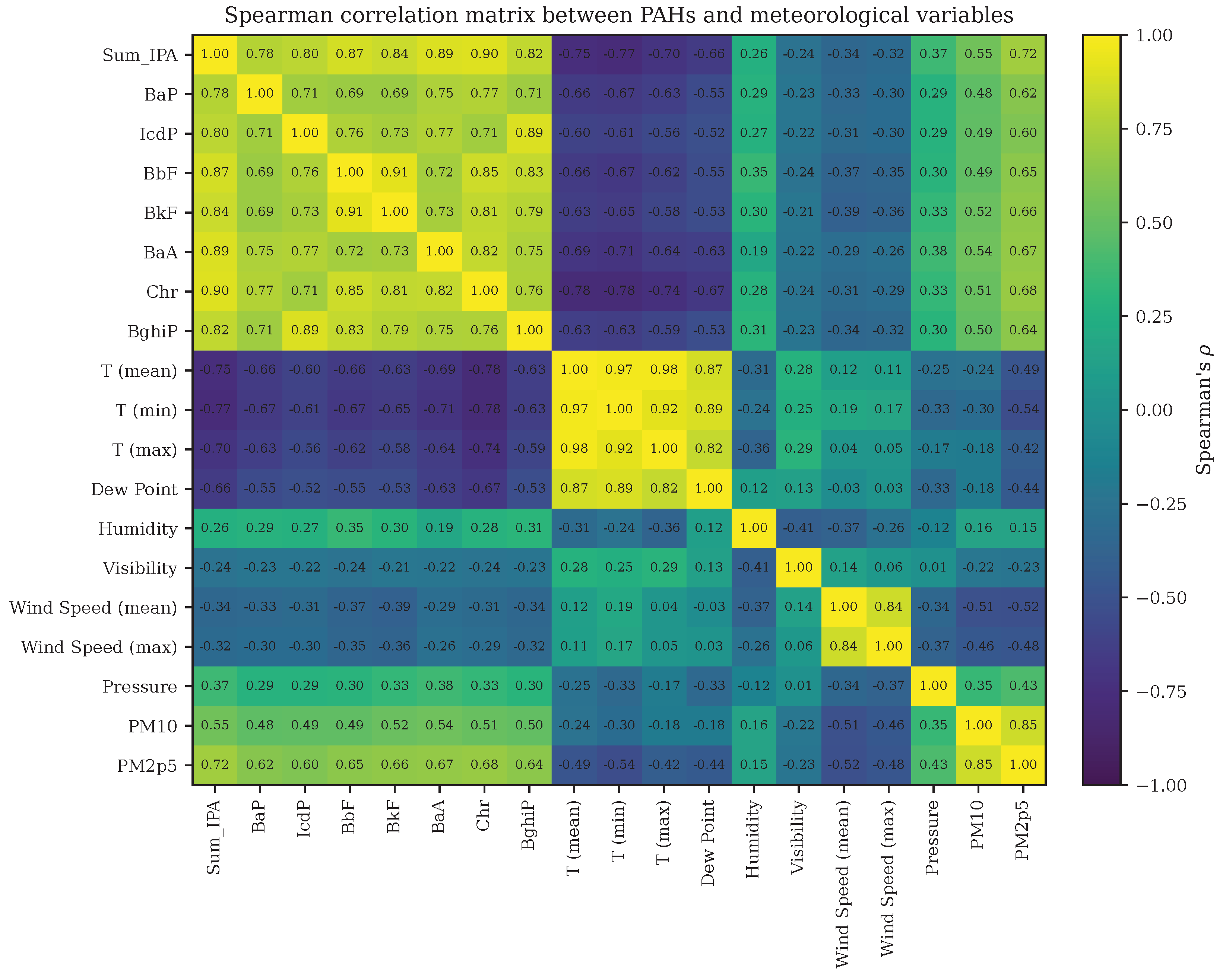
Statistically significant Spearman rank correlations (Table 4) were obtained between individual PAH congeners and meteorological variables. All HMW PAHs exhibited strong negative correlations with mean temperature (, ), reinforcing the dominant role of residential heating emissions during cold weather. Positive correlations with relative humidity (–) point to fog events and stable boundary-layer conditions as factors that promote PAH accumulation. Negative correlations with mean and maximum wind speed confirm efficient dilution under well-ventilated conditions, consistent with the established relationship between boundary-layer ventilation and urban aerosol concentrations [32].
3.6. Diagnostic Ratio Analysis
Figure 6 presents seasonal violin plots of the four diagnostic ratios computed from ST-smoothed time series. Bootstrapped mean values and 95% confidence intervals for all four ratios are reported in Table 5, where the very narrow intervals for IcdP/(IcdP+BghiP) and BaA/(BaA+Chr) indicate high reproducibility of these source-attribution signals, whereas the wider interval for BaP/BghiP (2.14 [1.77–2.55]) reflects its greater sensitivity to meteorological dilution and photochemical transformation.
Table 5.
Diagnostic ratios with bootstrap confidence intervals.
| Ratio | Mean (95% CI) |
|---|---|
| IcdP/(IcdP+BghiP) | 0.52 [0.51-0.52] |
| BaA/(BaA+Chr) | 0.54 [0.53-0.54] |
| Flu/(Flu+Pyr) | 0.38 [0.37-0.39] |
| BaP/BghiP | 2.14 [1.77-2.55] |
Bootstrap confidence intervals computed with 1000 iterations with replacement.
Fla/(Fla+Pyr).
Heating-season values clustered in the 0.50–0.60 range, consistent with coal and biomass combustion [13]. Non-heating-season values shifted to lower medians (approximately 0.45–0.50), overlapping the coal/traffic boundary but with a clear drift towards petroleum-combustion signatures.
BaP/BghiP.
The HS ratio was approximately 3.5× higher than in the NHS, reflecting the preferential emission of BaP relative to BghiP from biomass and coal combustion versus traffic-dominated periods [7]. HS median ratios exceeding unity confirm combustion-source dominance in winter.
IcdP/(IcdP+BghiP).
HS values above 0.50 are indicative of grass/wood burning and coal combustion, while NHS values near 0.40–0.50 are consistent with mixed petroleum combustion from traffic and mild stationary sources [13].
BaA/(BaA+Chr).
HS values above 0.35 confirm a pyrogenic origin; NHS values below 0.25 point to a stronger petrogenic or petroleum-combustion contribution typical of vehicle exhaust [2]. Violin plots reveal narrow winter distributions indicative of source homogeneity, and broader, occasionally multimodal summer distributions that reflect the co-occurrence of traffic, residual combustion, and episodic agricultural burning in transitional seasons.
3.7. Source Classification by Mixture Modelling
Application of the MML-SNOB algorithm to the HS four-dimensional ratio vector identified two dominant mixture classes accounting for % of samples. Class 1 (% of HS observations) is characterised by high , , and , consistent with residential biomass/solid-fuel combustion. Class 2 (% of HS observations) exhibits intermediate ratio values pointing to a mixed traffic-plus-heating source. A minor Class 3 (%) shows lower ratios consistent with petrogenic or heavy-fuel-oil combustion, possibly linked to port activities given the coastal character of the wider area.
For the NHS, the algorithm converged to two classes: a dominant class (%) with ratio values typical of gasoline and diesel vehicular combustion, and a secondary class (%) showing episodic biomass-burning signatures (e.g., agricultural waste burning in autumn). Cross-plot analysis is provided in Figure 7.
Figure 7.
Cross-plot of IcdP/(IcdP+BghiP) vs. BaA/(BaA+Chr) coloured by MML-SNOB class membership. Standard source-attribution regions from the literature [13] are superimposed.
Figure 7.
Cross-plot of IcdP/(IcdP+BghiP) vs. BaA/(BaA+Chr) coloured by MML-SNOB class membership. Standard source-attribution regions from the literature [13] are superimposed.
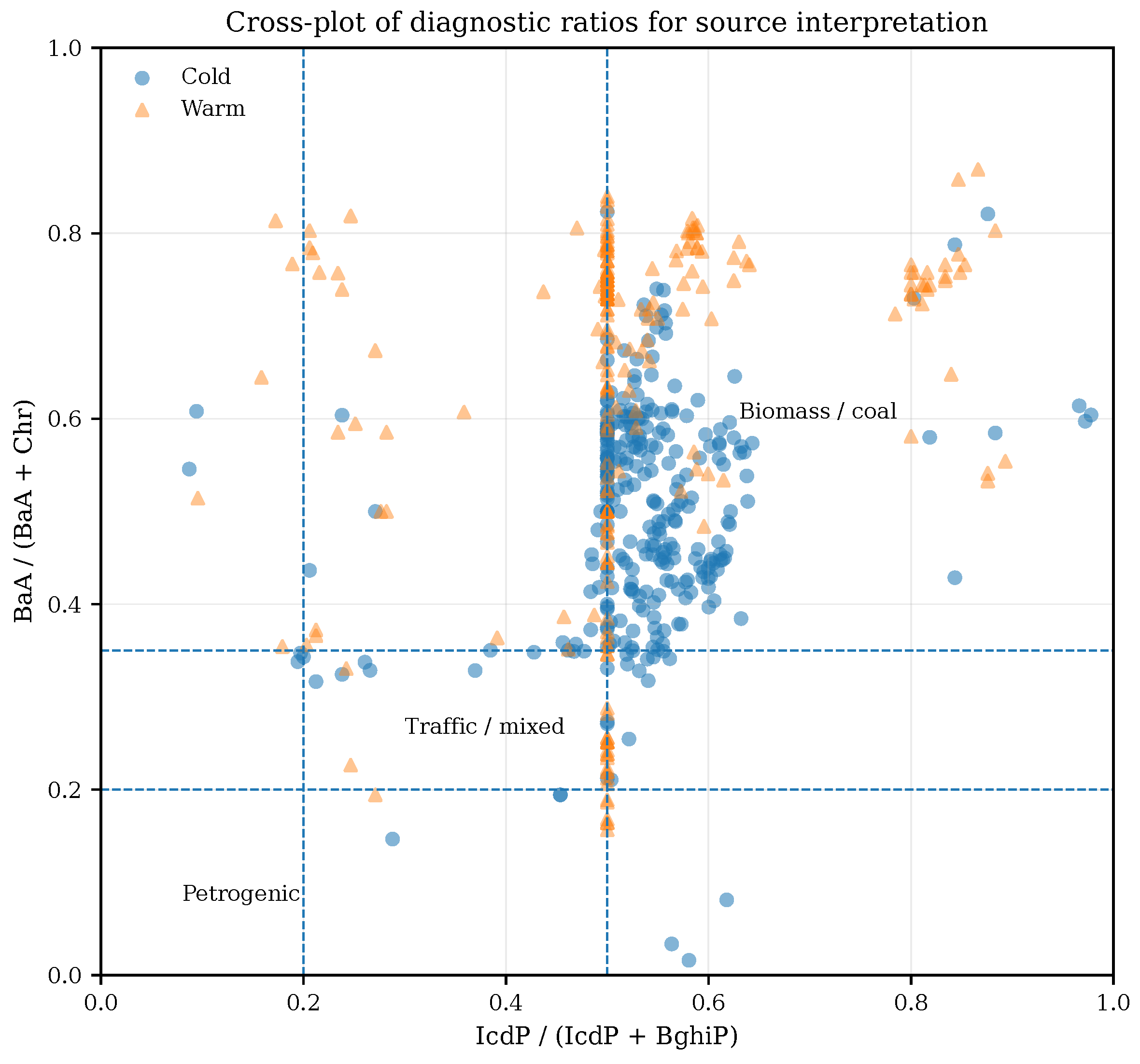
Figure 8.
Spearman correlation matrix between PAH congeners and meteorological variables. Only correlations with at are colour-coded.
Figure 8.
Spearman correlation matrix between PAH congeners and meteorological variables. Only correlations with at are colour-coded.
4. Discussion
4.1. Seasonal Dynamics and Comparison with the Literature
The winter enhancement of BaP documented here (winter-to-summer mean ratio of 10.1; Table 2) lies at the upper end of the range reported for Mediterranean and central European cities [1,7,14]. This is partly explained by the mild Campanian winters, during which wood-burning stoves and open fireplaces are used both as supplementary heaters and for recreational purposes, leading to a disproportionately strong biomass-combustion signal. Unlike northern European cities where coal combustion dominates the wintertime PAH signal [5], the ratio signatures at this site point primarily to biomass combustion, consistent with the near-absence of residential coal use in southern Italy. The BaP concentrations documented here (HS median ng m−3, peak 6.7 ng m−3) substantially exceed the EU annual target of 1 ng m−3 [4] on many individual winter days, underlining the public health relevance of short-term stagnation episodes and the need for monitoring strategies able to capture these transient extremes.
The dominance of residential biomass and wood combustion during the heating season is consistent with independent radiocarbon-based source apportionment conducted in the historic centre of Naples, approximately 15 km south-west of Pomigliano d’Arco. Sirignano et al. [33] showed that primary biomass-burning carbon accounts for about 31% of total carbon (roughly 15% of PM2.5 mass) during winter, while fossil fuel sources contribute less than one third of total carbon. This regional-scale evidence supports the interpretation that biomass combustion is a major driver of wintertime PAH loadings in the wider Naples metropolitan area.
The PAH-to-PM2.5 mass ratios reported in Table 3 add a compositional perspective to the seasonal contrast discussed above. The 2–4.6-fold increase in PAH/PM2.5 ratios from non-heating to heating season implies that not only does total PM2.5 mass increase in winter, but the particle matrix also becomes chemically enriched in mutagenic PAHs independently of the mass effect. This dual amplification – higher PM2.5 mass and higher PAH fraction per unit mass – helps explain why heating-season BaPTEQ exceeds the non-heating season value by nearly an order of magnitude, whereas absolute PM2.5 concentrations differ by a factor of only about five (Table 1). From a health-risk perspective, population exposure during winter stagnation episodes is therefore penalised twice: a larger inhaled particle mass combined with a higher carcinogenic potency per unit mass.
At a broader scale, our findings are consistent with the picture emerging from data-assimilation studies over Northern Italy. Using a Bayesian hierarchical framework, Chianese et al. [12] showed that PM10 annual mean concentrations in the Po Valley frequently exceed or approach the EU limit of 40 g m−3, with a large fraction of the population exposed to levels above WHO interim targets. While the present study focuses on a single Mediterranean urban site and on PM2.5-bound PAHs, both analyses point to a persistent regional burden of particulate pollution with significant implications for public health.
The anomalous DahA inversion (HS/NHS = 0.71) is consistent with the source-attribution results obtained from MML-SNOB. While biomass combustion dominates DahA emissions in absolute terms during winter, the relative DahA enrichment in summer PM2.5 confirms the persistent contribution of traffic-related sources throughout the year, a signal that is also visible in the residual component of the time-series decomposition. In future receptor modelling applications, the contrasting seasonal behaviour of DahA versus BbF and BaP could be exploited as an additional discriminant between traffic and biomass-combustion source profiles.
4.2. Health Risk Implications
The heating-season ILCR values quantified in Section 3.2 () place Pomigliano d’Arco within the potential-to-high risk tier (–) documented across a broad range of urban and industrial environments worldwide [6]. This upper-end positioning within the Mediterranean range is consistent with findings from southern European coastal cities where residential wood combustion coexists with urban traffic under conditions of episodic boundary-layer suppression [7,24]. The disproportionate contribution of the heating season to the annual risk burden (> 80% of the annual-average ILCR concentrated in four winter months) reinforces the public health case for targeting residential biomass combustion as the single highest-priority abatement measure. Although the present study does not resolve the ultrafine fraction (), the literature consistently demonstrates that HMW congeners — which dominate the BaPTEQ in this dataset — are predominantly associated with the PM2.5 and sub-micrometre fractions [28,31], and that the ultrafine fraction carries a disproportionately high PAH burden per unit mass [6]. Consequently, the ILCR estimates reported here should be regarded as conservative lower bounds. Future investigations incorporating parallel size-resolved sampling would strengthen the exposure assessment and facilitate direct comparison with the emerging literature on ultrafine-particle PAH risk.
4.3. Role of Meteorology
Temperature acts as the dominant meteorological driver, simultaneously controlling residential heating demand and atmospheric stability. The independent contributions of wind speed (ventilation/dilution) and relative humidity (boundary-layer stability, fog formation) indicate that episode severity is jointly determined by emission strength and dispersion conditions [32]. Fog events recorded on several winter days likely enhanced scavenging of gas-phase PAHs onto droplets, but the net effect on PM2.5-bound concentrations depends on the balance between increased boundary-layer confinement and enhanced wet deposition — a mechanistic interplay that merits dedicated future investigation.
4.4. COVID-19 Lockdown as a Natural Experiment
The near-complete suppression of HMW-PAH signals during the Italian national lockdown (9 March–4 May 2020) provides one of the most direct observational demonstrations available in the Mediterranean literature of the dominance of anthropogenic activity over natural and long-range transport contributions to non-heating-season PAH loading [16,17]. The residual near-background floor of approximately 0.8 ng m-3 for PAH quantified under conditions of near-complete traffic cessation is broadly consistent with background levels inferred in comparable lockdown studies conducted in northern Italian cities [17,34], and provides a useful lower-bound reference for evaluating the efficacy of future emission control interventions.
The integration of toxic equivalency factors and the inhalation unit risk provides a direct bridge from atmospheric measurements to health risk assessment [26]. The Monte Carlo approach propagates observational variability through the risk calculation, yielding probabilistic ILCR estimates rather than single deterministic values. Winter exposure contributes disproportionately to the annual risk burden, an observation with direct implications for the timing and targeting of regulatory interventions.
4.5. Methodological Contributions and Future Directions
The probabilistic source classification achieved through the MML-SNOB algorithm represents an intermediate step towards full mass-balance receptor modelling. As recommended by Safo-Adu et al. [6] and Dat and Chang [28], ratio-based source attribution should ideally be complemented by Positive Matrix Factorisation (PMF) applied to the complete 16-congener concentration matrix, which provides quantitative source apportionment with mass-balance constraints and explicit uncertainty estimation via bootstrap resampling [35]. The three-year daily dataset presented here constitutes a robust foundation for such an extension, particularly if augmented with additional chemical markers — e.g., levoglucosan or water-soluble potassium for biomass combustion, and hopanes or elemental carbon for vehicular emissions — to improve source profile resolution and reduce cross-contamination between the residential-heating and traffic-related factors. The complementary soil-based PAH inventory available for rural Campania [15] could serve as an additional constraint for source profiles in future receptor modelling efforts.
The combination of a missing-value-robust moving-average decomposition, bootstrap uncertainty quantification, and MML-SNOB mixture modelling constitutes a methodologically coherent and reproducible framework for multi-year PAH datasets with irregular data gaps. Unlike conventional threshold-based ratio classification [13], the MML approach furnishes explicit posterior class-membership probabilities, an objective model-selection criterion, and automatic uncertainty quantification. The seasonal shift in class composition — from combustion-dominant in winter to traffic-dominant in summer — is physically coherent and aligns with both the ratio analysis and the meteorological correlations.
The strong seasonal concentration of PAH exposure suggests that targeted interventions during the heating season could yield substantial health benefits. Reducing emissions from residential biomass combustion emerges as the single highest-priority action, given that Class 1 combustion sources account for ≈58% of heating-season observations. At the same time, the persistence of a residual background signal means that traffic and industrial emissions remain relevant throughout the year, calling for continuous mitigation strategies alongside seasonal measures.
5. Conclusions
A three-year daily monitoring campaign of 16 PM2.5-bound PAH congeners at the Pomigliano d’Arco monitoring site in the Naples metropolitan area has yielded the following main findings.
- 1.
- A pronounced and statistically robust seasonal cycle, with winter-to-summer mean ratios ranging from 2.6 (DahA) to 10.1 (BaP) and median concentrations up to 12× higher in the heating season, driven primarily by residential biomass combustion.
- 2.
- BaP peak concentrations reaching 6.7 ng m−3 during meteorological stagnation episodes — well above the EU annual target of 1 ng m−3 — with associated heating-season ILCR values of , two orders of magnitude above the acceptable risk threshold.
- 3.
- The iterative missing-value-robust moving-average decomposition revealed that the residual PAH component (RT) retains a persistent winter-to-summer ratio of 2–4 after removal of the primary seasonal cycle, indicating the presence of year-round baseline sources — predominantly traffic and industrial emissions — whose contribution is partially masked by the dominant heating-season signal in raw concentration data.
- 4.
- Strong negative Spearman correlations of all HMW congeners with air temperature () and wind speed, and positive correlations with relative humidity, quantifying the meteorological modulation of PAH episode intensity.
- 5.
- A clear lockdown fingerprint in spring 2020 demonstrating that near-background PAH conditions ( ng m−3) are achievable when anthropogenic activities are substantially suppressed, with concentrations ≈85% below the seasonal prediction.
- 6.
- A novel application of the MML-SNOB Bayesian mixture model to diagnostic PAH ratios, identifying residential biomass combustion as the dominant winter source class (% of HS samples) and vehicular emissions as the dominant summer class (% of NHS samples), supported by bootstrap-validated diagnostic ratios (Table 5).
These results advance the characterisation of PAH pollution in the undersampled southern Mediterranean and provide an empirical basis for season-specific emission control policies, with particular emphasis on regulating residential biomass combustion during winter atmospheric stagnation events.
Supplementary Materials
The following supporting information can be downloaded at the website of this paper posted on Preprints.org.
Author Contributions
Conceptualisation M.T.; methodology, A.G., E.C. A.R. and M.T.; software, A.R.; validation, A.R., A.G. and E.C.; formal analysis, E.E. and E.C.; investigation, E.E., M.A. and A.G.; data curation, M.A., E.E., E.C.; writing original draft preparation, E.C., M.T. and A.R.; writing—review and editing, E.C and A.R.; project administration, M.T. All authors have read and agreed to the published version of the manuscript.
Funding
This research received no external funding.
Institutional Review Board Statement
Not applicable.
Informed Consent Statement
Not applicable.
Data Availability Statement
The dataset and the python programs used to develop figures and tables enclosed in this work are available on Zenodo, on the following doi number: 10.5281/zenodo.19692361.
Acknowledgments
The authors would like to thank the Municipality of Pomigliano d’Arco for providing the sampling site.
Conflicts of Interest
The authors declare no conflicts of interest.
References
- Yang, L.; Zhang, H.; Zhang, X.; et al. Exposure to atmospheric particulate matter-bound polycyclic aromatic hydrocarbons and their health effects: A review. Int. J. Environ. Res. Public Health 2021, 18, 2177. [Google Scholar] [CrossRef] [PubMed]
- National Toxicology Program. Polycyclic Aromatic Hydrocarbons: 15 Listings. Report on Carcinogens, Fifteenth Edition; National Institute of Environmental Health Sciences (NIEHS): Research Triangle Park, NC, USA, 2021. [Google Scholar]
- IARC Working Group. Chemical Agents and Related Occupations. IARC Monographs on the Evaluation of Carcinogenic Risks to Humans, Volume 100F; International Agency for Research on Cancer: Lyon, France, 2012. [Google Scholar]
- European Parliament and Council of the European Union. Directive 2004/107/EC of the European Parliament and of the Council of 15 December 2004 Relating to Arsenic, Cadmium, Mercury, Nickel and Polycyclic Aromatic Hydrocarbons in Ambient Air. Off. J. Eur. Union 2004, L 23, 3–16. [Google Scholar]
- European Environment Agency (EEA). Air Quality in Europe – 2018 Report. 2018. [Google Scholar]
- Safo-Adu, G.; Attiogbe, F.; Emahi, I.; Ofosu, F. A review of the sources, distribution sequences, and health risks associated with exposure to atmospheric polycyclic aromatic hydrocarbons. Cogent Eng. 2023, 10, 2199511. [Google Scholar] [CrossRef]
- Tsiodra, I.; Grivas, G.; Tavernaraki, K.; Bougiatioti, A.; Apostolaki, M.; Paraskevopoulou, D.; Tsagkaraki, M.; Zarmpas, P.; Oikonomou, K.; Theodosi, C.; et al. Annual Exposure to Polycyclic Aromatic Hydrocarbons in Urban Environments Linked to Idling Automobiles and Biomass Burning. Atmos. Chem. Phys. 2021, 21, 17865–17883. [Google Scholar] [CrossRef]
- Riccio, A.; Chianese, E.; Monaco, D.; Costagliola, M.; Perretta, G.; Prati, M.; Agrillo, G.; Esposito, A.; Gasbarra, D.; Shindler, L.; et al. Real-world automotive particulate matter and PAH emission factors and profile concentrations: Results from an urban tunnel experiment in Naples, Italy. Atmos. Environ. 2016, 141, 379–387. [Google Scholar] [CrossRef]
- Riccio, A.; Chianese, E.; Tirimberio, G.; Prati, M.V. Emission Factors of Inorganic Ions from Road Traffic: A Case Study from the City of Naples (Italy). Transp. Res. Part D. Transp. Environ. 2017, 54, 239–249. [Google Scholar] [CrossRef]
- Chianese, E.; Tirimberio, G.; Riccio, A. PM2.5 and PM10 in the Urban Area of Naples: Chemical Composition, Chemical Properties and Influence of Air Masses Origin. J. Atmos. Chem. 2019, 76, 151–169. [Google Scholar] [CrossRef]
- Chianese, E.; Tirimberio, G.; Appolloni, L.; Dinoi, A.; Contini, D.; Di Gilio, A.; Palmisani, J.; Cotugno, P.; Miniero, D.V.; Dusek, U.; et al. Chemical characterisation of PM10 from ship emissions: a study on samples from hydrofoil exhaust stacks. Environ. Sci. Pollut. Res. 2022, 29, 17723–17736. [Google Scholar] [CrossRef]
- Chianese, E.; Galletti, A.; Giunta, G.; Landi, T.; Marcellino, L.; Montella, R.; Riccio, A. Spatiotemporally resolved ambient particulate matter concentration by fusing observational data and ensemble chemical transport model simulations. Ecol. Model. 2018, 385, 173–181. [Google Scholar] [CrossRef]
- Yunker, M.B.; Macdonald, R.W.; Vingarzan, R.; Mitchell, R.H.; Goyette, D.; Sylvestre, S. PAHs in the Fraser River Basin: A Critical Appraisal of PAH Ratios as Indicators of PAH Source and Composition. Org. Geochem. 2002, 33, 489–515. [Google Scholar] [CrossRef]
- Siudek, P. Seasonal distribution of PM2. 5-bound polycyclic aromatic hydrocarbons as a critical indicator of air quality and health impact in a coastal-urban region of Poland. Sci. Total Environ. 2022, 827, 154375. [Google Scholar] [CrossRef]
- Monaco, D.; Riccio, A.; Chianese, E.; Adamo, P.; Di Rosa, S.; Fagnano, M. Chemical Characterization and Spatial Distribution of PAHs and Heavy Hydrocarbons in Rural Sites of Campania Region, South Italy. Environ. Sci. Pollut. Res. 2015, 22, 14993–15003. [Google Scholar] [CrossRef]
- Collivignarelli, M.C.; Abbà, A.; Bertanza, G.; Pedrazzani, R.; Ricciardi, P.; Carnevale Miino, M. Lockdown for CoViD-2019 in Milan: What Are the Effects on Air Quality? Sci. Total Environ. 2020, 732, 139280. [Google Scholar] [CrossRef] [PubMed]
- Pala, D.; Baj, A.; Strano, S.; Manzoni, A.; Salinelli, G.; Rossi, V.; Ferrante, S. Impact of COVID-19 Lockdown on PM Concentrations in an Italian Northern City: A Study in Pavia Using 23 Air Quality Sensors. PLoS ONE 2022, 17, e0263265. [Google Scholar] [CrossRef]
- Solazzo, E.; Riccio, A.; Van Dingenen, R.; Valentini, L.; Galmarini, S. Evaluation and Uncertainty Estimation of the Impact of Air Quality Modelling on Crop Yields and Premature Deaths Using a Multi-model Ensemble. Sci. Total Environ. 2018, 633, 1437–1452. [Google Scholar] [CrossRef] [PubMed]
- U.S. Environmental Protection Agency. Method 8000D: Determinative Chromatographic Separations. Technical Report, 2014. SW-846 Update V.
- Helsel, D.R. Statistics for censored environmental data using Minitab and R; John Wiley & Sons, 2011; Vol. 77. [Google Scholar]
- Zurbenko, I.G.; Smith, D. Kolmogorov–Zurbenko filters in spatiotemporal analysis. Wiley Interdiscip. Rev. Comput. Stat. 2018, 10, e1419. [Google Scholar] [CrossRef]
- Moisan, S. nanconvn: MATLAB Convolution Correcting for NaN Values. MATLAB File Exch. 2013. [Google Scholar]
- World Health Organization. Air Quality Guidelines for Europe. WHO Regional Publications, European Series No. 91, 2000.
- Sánchez-Piñero, J.; Moreda-Piñeiro, J.; Turnes-Carou, I.; Fernández-Amado, M.; Muniategui-Lorenzo, S.; López-Mahía, P. Polycyclic aromatic hydrocarbons in atmospheric particulate matter (PM10) at a Southwestern Europe coastal city: status, sources and health risk assessment. Air Qual. Atmos. Health 2021, 14, 1325–1339. [Google Scholar] [CrossRef]
- U.S. Environmental Protection Agency. Exposure Factors Handbook: 2011 Edition. EPA/600/R-09/052F, 2011.
- Nisbet, I.C.; Lagoy, P.K. Toxic equivalency factors (TEFs) for polycyclic aromatic hydrocarbons (PAHs). Regul. Toxicol. Pharmacol. 1992, 16, 290–300. [Google Scholar] [CrossRef]
- EFSA Panel on Contaminants in the Food Chain. Polycyclic Aromatic Hydrocarbons in Food. EFSA J. 2008, 724, 1–114.
- Dat, N.; Chang, M. Review on characteristics of PAHs in atmosphere, anthropogenic sources and control technologies. Sci. Total Environ. 2017, 609, 682–693. [Google Scholar] [CrossRef]
- Wallace, C.S.; Dowe, D.L. MML Mixture Modelling of Multi-state, Poisson, vonMises Circular and Gaussian Distributions. Proceedings of the Proceedings of the Sixth International Workshop on Artificial Intelligence and Statistics 1997, Vol. R1, PMLR, 529–536. [Google Scholar]
- Dale, M.; Allison, L.; Dale, P. Model selection using Minimal Message Length: an example using pollen data. Community Ecol. 2010, 11, 187–201. [Google Scholar] [CrossRef]
- Liang, B.; et al. Size distribution of particulate PAHs and their health risks: a review. J. Environ. Sci. 2020, 88, 370–384. [Google Scholar] [CrossRef]
- Stull, R.B. An Introduction to Boundary Layer Meteorology; Springer Science & Business Media, 1988. [Google Scholar]
- Sirignano, C.; Riccio, A.; Chianese, E.; Ni, H.; Zenker, K.; D’Onofrio, A.; Meijer, H.A.; Dusek, U. High contribution of biomass combustion to PM2. 5 in the city centre of Naples (Italy). Atmosphere 2019, 10, 451. [Google Scholar] [CrossRef]
- Altuwayjiri, A.; Soleimanian, E.; Moroni, S.; Palomba, P.; Borgini, A.; De Marco, C.; Sioutas, C. The Impact of Stay-Home Policies during Coronavirus-19 Pandemic on the Chemical and Toxicological Characteristics of Ambient PM2.5 in the Metropolitan Area of Milan, Italy. Sci. Total Environ. 2021, 758, 143582. [Google Scholar] [CrossRef]
- Paatero, P.; Tapper, U. Positive Matrix Factorization: A Non-Negative Factor Model with Optimal Utilization of Error Estimates of Data Values. Environmetrics 1994, 5, 111–126. [Google Scholar] [CrossRef]
Figure 1.
Location of the monitoring site in Pomigliano d’Arco (red dot), approximately 15 km north-east of Naples. The inset shows the regional location within southern Italy. Road network and urban features were derived from OpenStreetMap data.
Figure 1.
Location of the monitoring site in Pomigliano d’Arco (red dot), approximately 15 km north-east of Naples. The inset shows the regional location within southern Italy. Road network and urban features were derived from OpenStreetMap data.
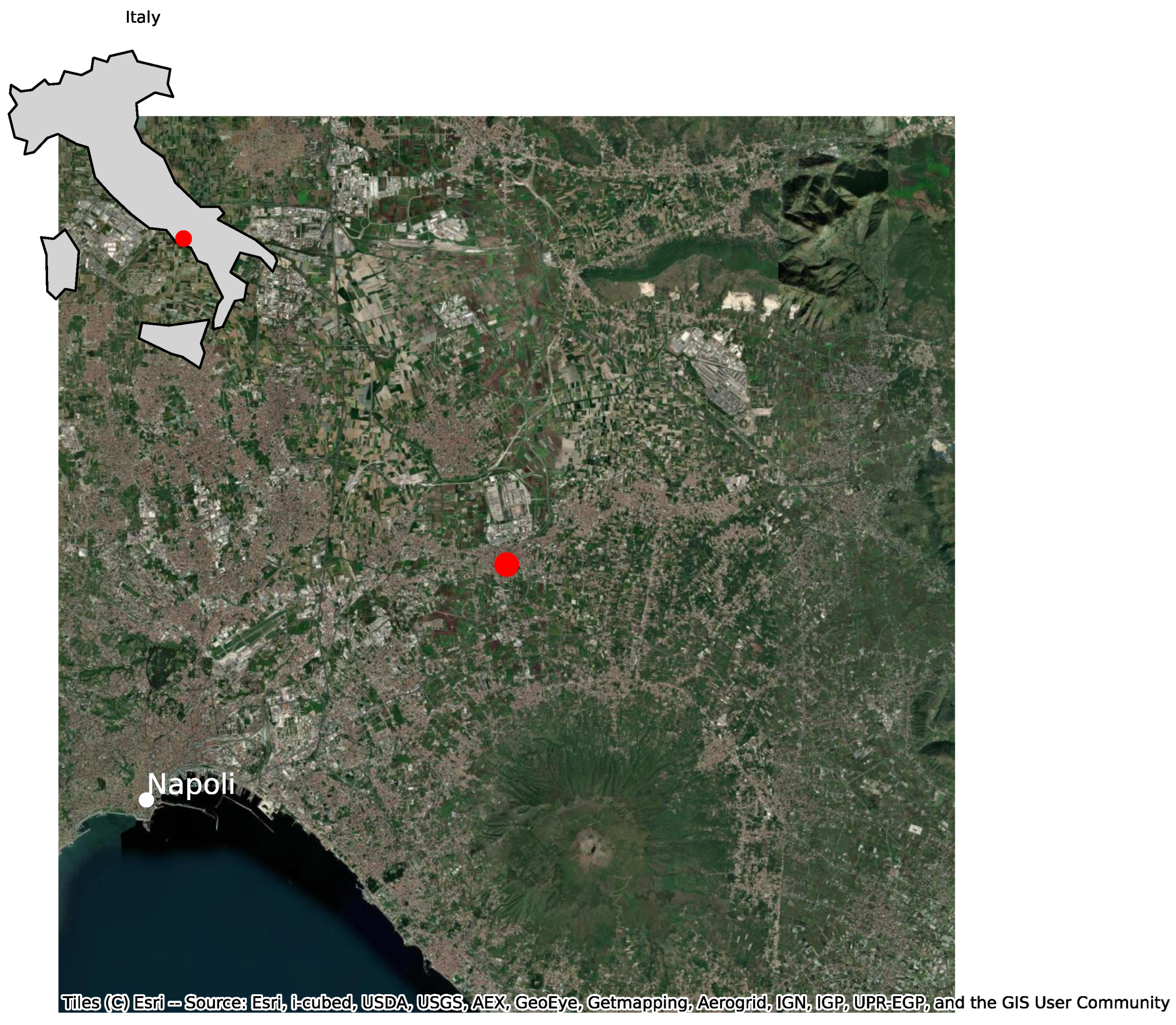
Figure 2.
Monthly mean seasonal components from time-series decomposition. Error bars represent bootstrap 95% confidence intervals (1000 iterations with replacement).
Figure 2.
Monthly mean seasonal components from time-series decomposition. Error bars represent bootstrap 95% confidence intervals (1000 iterations with replacement).
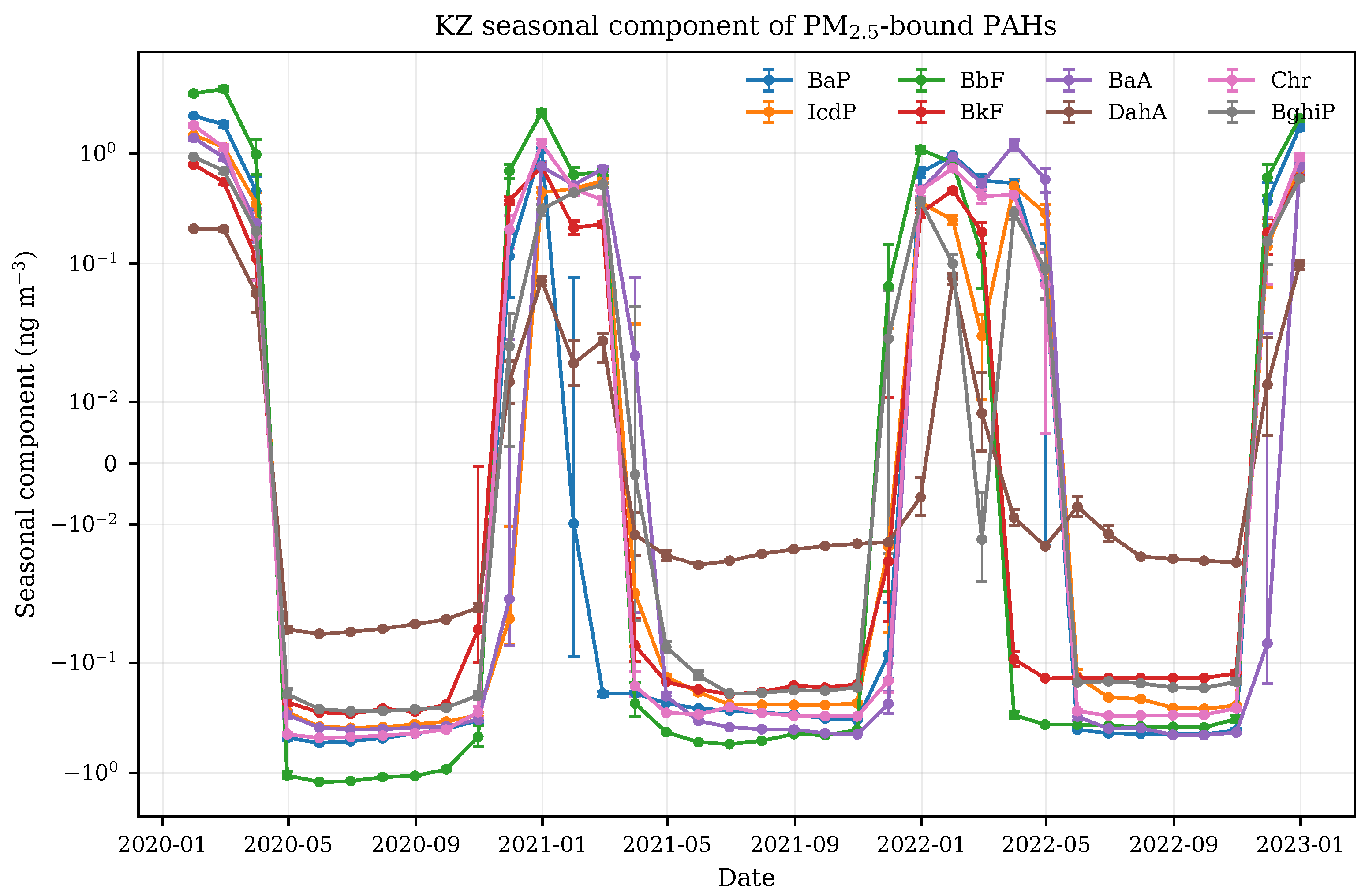
Figure 3.
Residual components (RT) representing episode-scale variability not explained by the seasonal or trend signals, for selected HMW PAH congeners and PM2.5.
Figure 3.
Residual components (RT) representing episode-scale variability not explained by the seasonal or trend signals, for selected HMW PAH congeners and PM2.5.
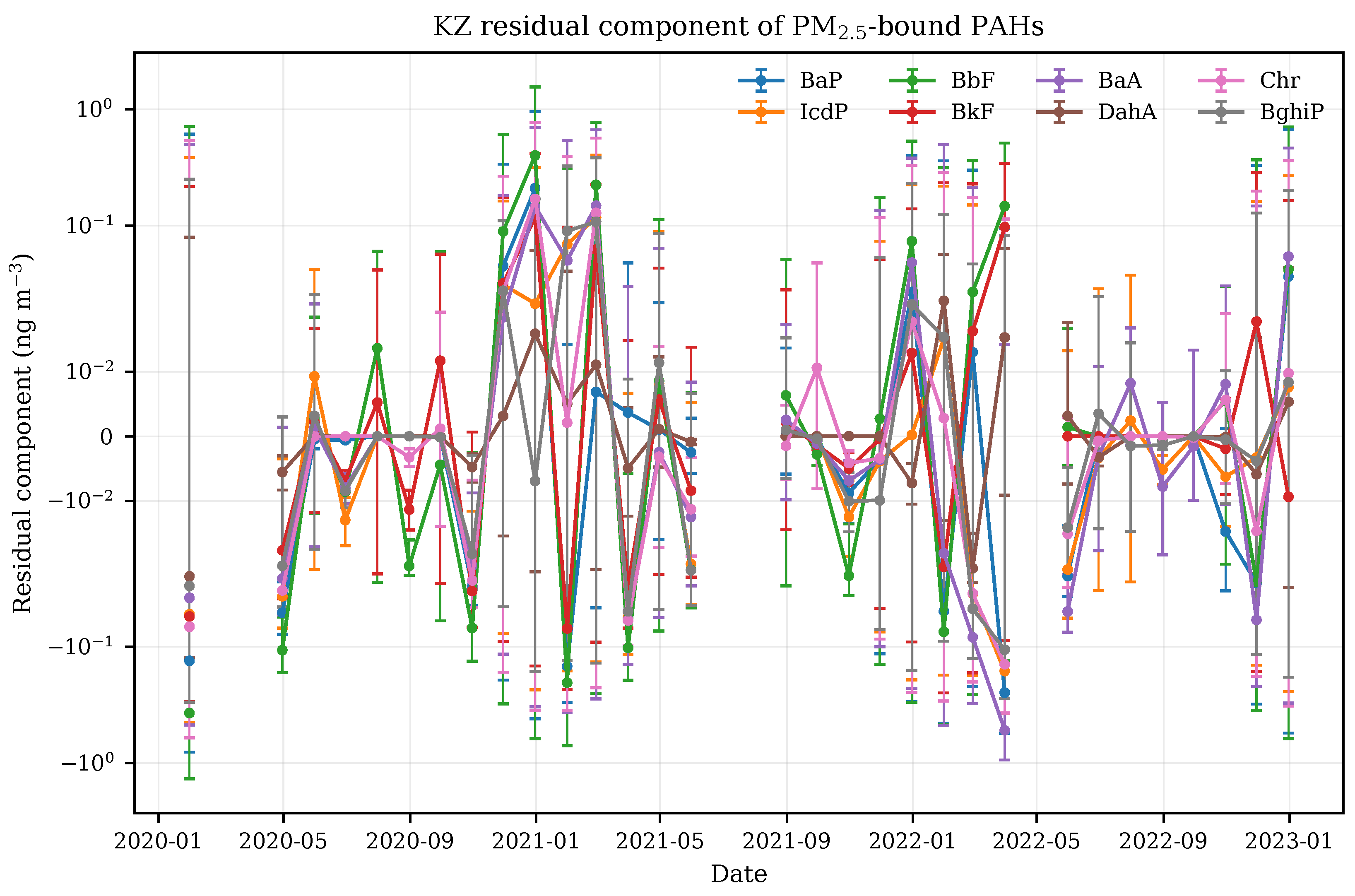
Figure 4.
Zoomed time series of total PAHs during 2020. The shaded region indicates the COVID-19 lockdown period (9 March – 4 May 2020), during which concentrations dropped to near-detection levels (% below the seasonal baseline).
Figure 4.
Zoomed time series of total PAHs during 2020. The shaded region indicates the COVID-19 lockdown period (9 March – 4 May 2020), during which concentrations dropped to near-detection levels (% below the seasonal baseline).
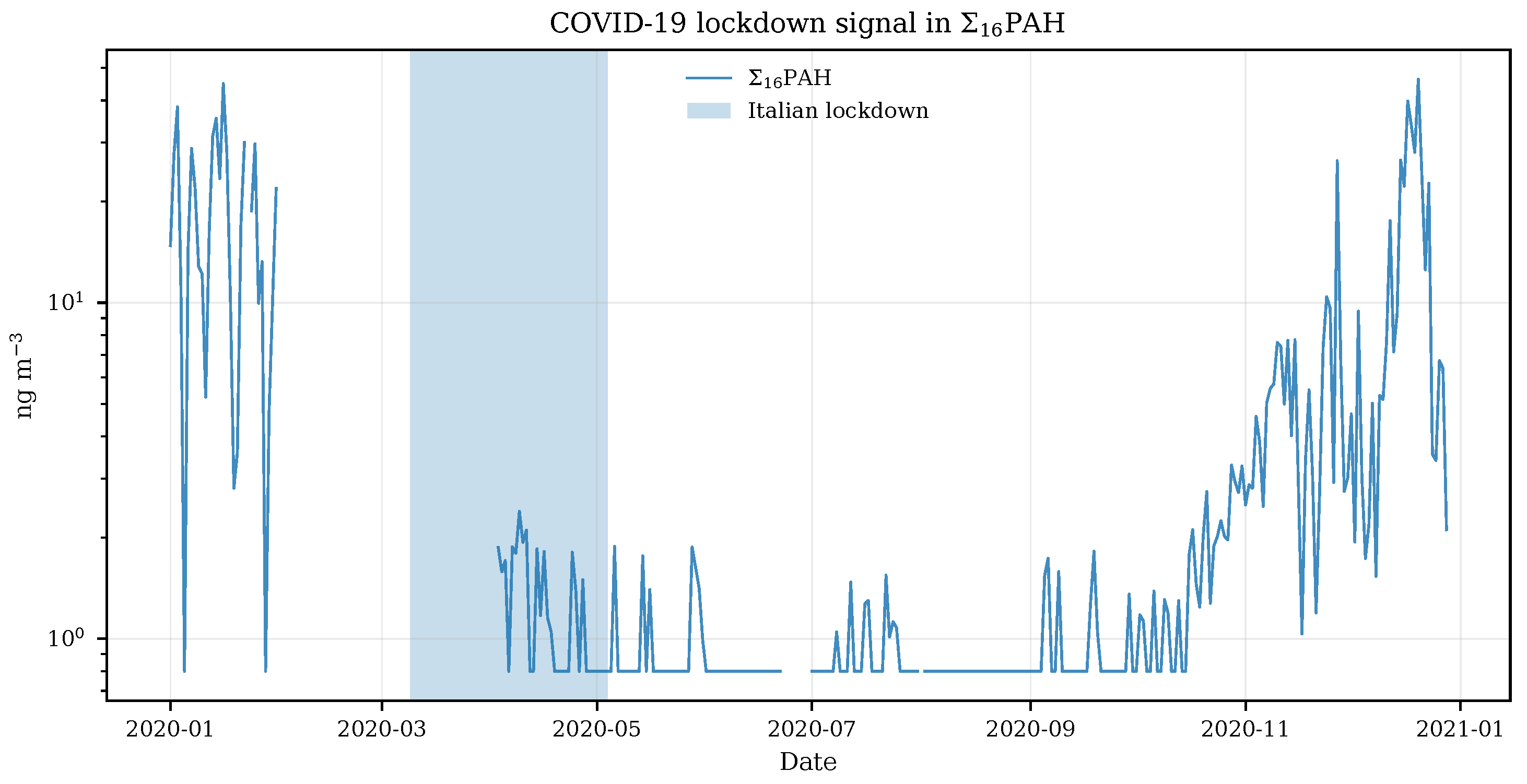
Figure 5.
Time series of PAH and BaP concentrations over 2020–2022. Shaded areas indicate bootstrap 95% confidence intervals. The grey band marks the COVID-19 lockdown period.
Figure 5.
Time series of PAH and BaP concentrations over 2020–2022. Shaded areas indicate bootstrap 95% confidence intervals. The grey band marks the COVID-19 lockdown period.
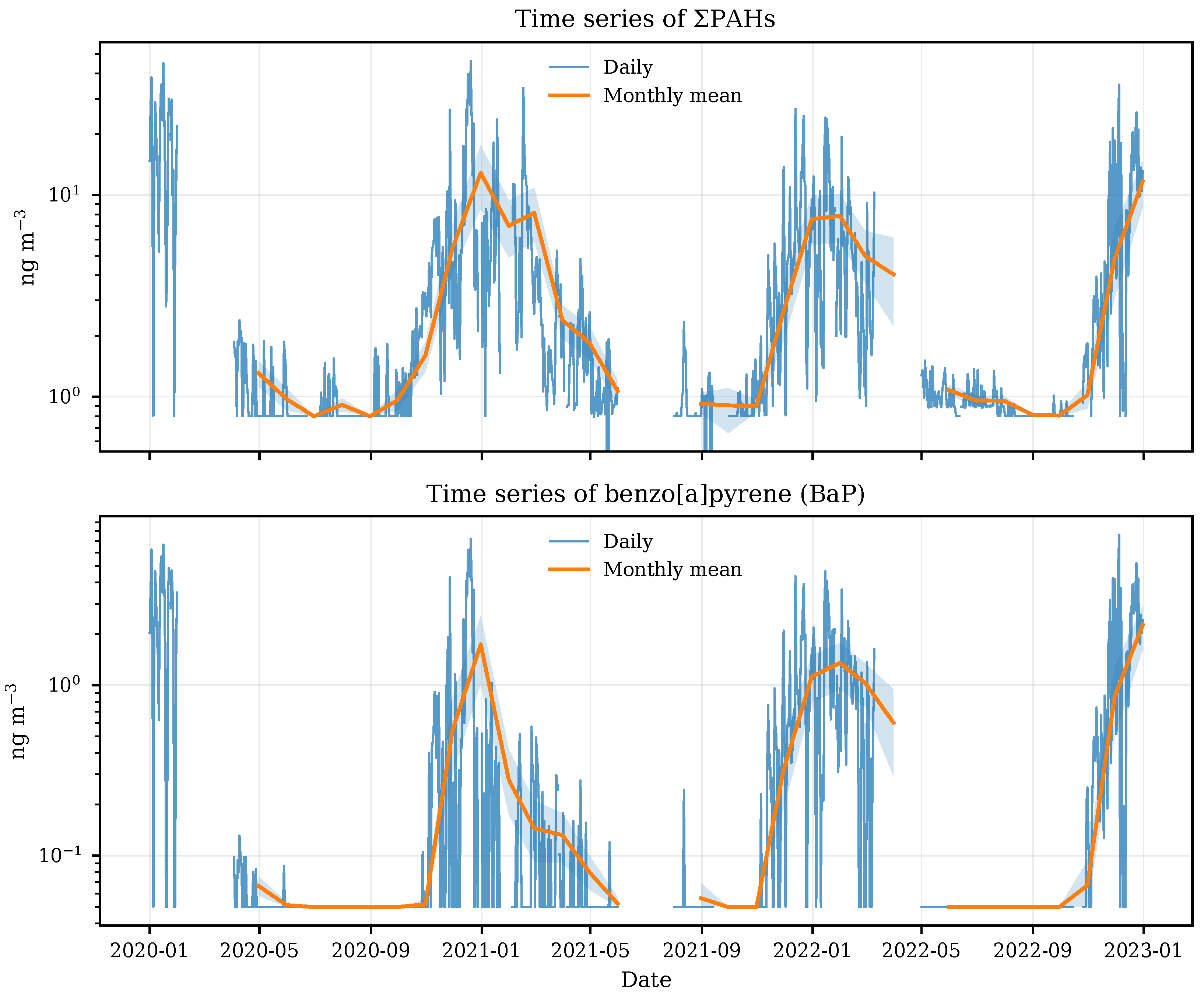
Figure 6.
Violin plots of the four diagnostic PAH ratios stratified by heating season (HS, November–February) and non-heating season (NHS, March–October). Bootstrap 95% confidence intervals are shown for the seasonal medians.
Figure 6.
Violin plots of the four diagnostic PAH ratios stratified by heating season (HS, November–February) and non-heating season (NHS, March–October). Bootstrap 95% confidence intervals are shown for the seasonal medians.
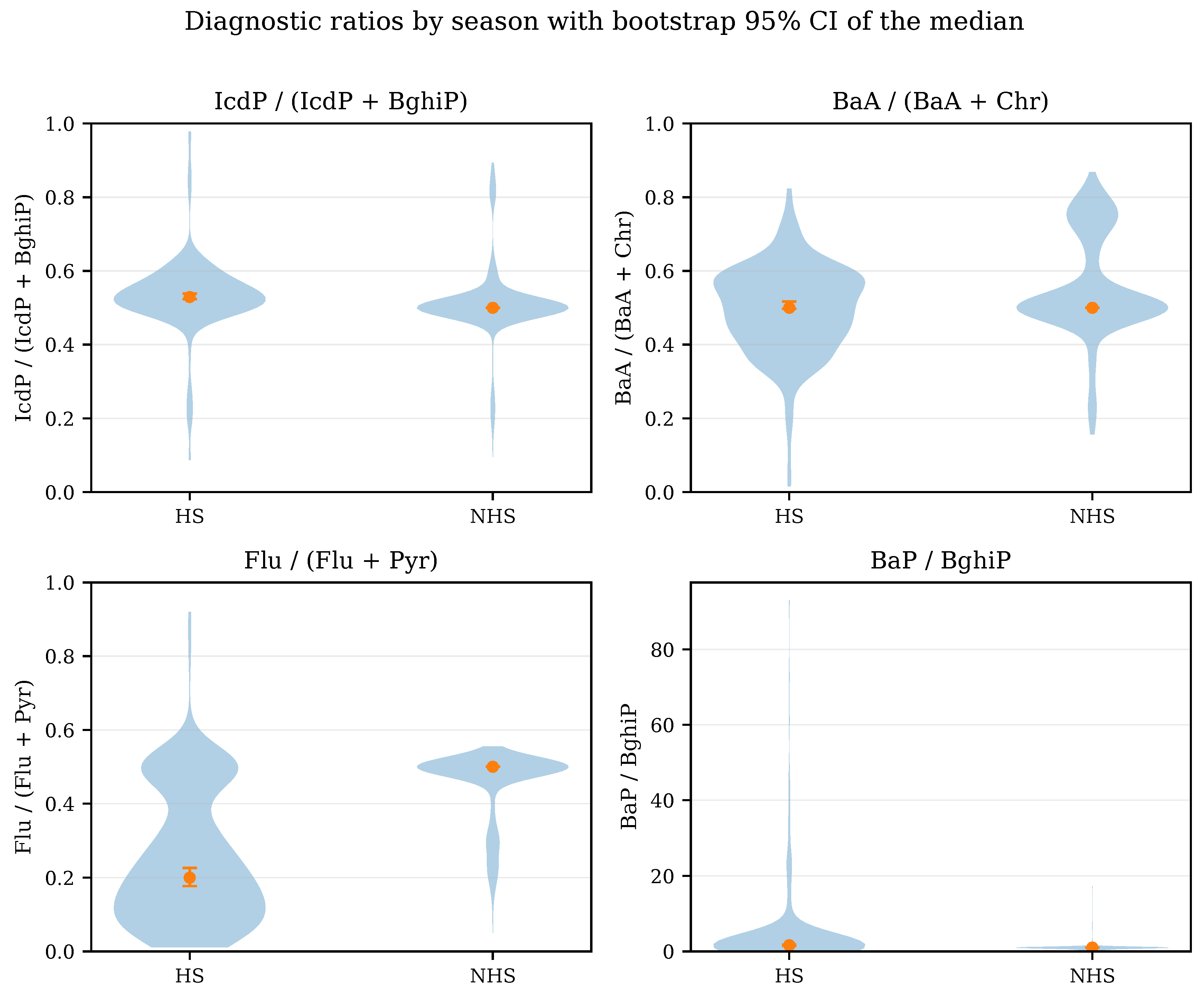
Table 1.
Seasonal statistics median and inter-quartile range (IQR; expressed as – interval, ng m−3 for PAHs and g m−3 for PM2.5) of PAH, BaP, IcdP, BbF, BkF, BaA, DahA, Chr, BghiP, and PM2.5 at the Pomigliano d’Arco monitoring site (2020–2022). Concentrations in ng m−3 (PAH) and g m−3 (PM2.5). HS = heating season (Nov–Feb); NHS = non-heating season (Mar–Oct).
Table 1.
Seasonal statistics median and inter-quartile range (IQR; expressed as – interval, ng m−3 for PAHs and g m−3 for PM2.5) of PAH, BaP, IcdP, BbF, BkF, BaA, DahA, Chr, BghiP, and PM2.5 at the Pomigliano d’Arco monitoring site (2020–2022). Concentrations in ng m−3 (PAH) and g m−3 (PM2.5). HS = heating season (Nov–Feb); NHS = non-heating season (Mar–Oct).
| Parameter | Heating Season (HS) | Non-Heating Season (NHS) | ||
|---|---|---|---|---|
| Median | IQR | Median | IQR | |
| PAH | 10.4 | 4.7–21.9 | 0.8 | 0.8–1.9 |
| BaP | 2.5 | 0.9–4.7 | <0.05 | <0.05–0.05 |
| IcdP | 1.9 | 0.5–3.6 | <0.05 | <0.05–0.05 |
| BbF | 5.2 | 2.0–8.7 | <0.05 | <0.05–0.10 |
| BkF | 1.6 | 0.6–2.4 | <0.05 | <0.05–0.05 |
| BaA | 3.1 | 0.8–5.0 | <0.05 | <0.05–0.15 |
| DahA | 0.8 | 0.05–1.6 | <0.05 | <0.05–0.05 |
| Chr | 4.1 | 1.3–6.1 | 0.05 | <0.05–0.15 |
| BghiP | 1.3 | 0.4–2.2 | <0.05 | <0.05–0.05 |
| PM2.5 | 72 | 40–107 | 14 | 9–20 |
Table 3.
Seasonal PAH-to-PM2.5 mass ratios with log-transformed bootstrap 95% confidence intervals.
| Compound | HS (95% CI) | NHS (95% CI) | HS/NHS |
|---|---|---|---|
| BaP | 0.012 [0.011-0.014] | 0.0036 [0.0034-0.0037] | 3.5 |
| BbF | 0.023 [0.02-0.027] | 0.005 [0.0046-0.0053] | 4.6 |
| BkF | 0.0094 [0.0085-0.01] | 0.0041 [0.0039-0.0043] | 2.3 |
| IcdP | 0.01 [0.0089-0.011] | 0.0043 [0.0041-0.0045] | 2.3 |
| BghiP | 0.0087 [0.0078-0.0097] | 0.0041 [0.0039-0.0043] | 2.1 |
| BaA | 0.014 [0.013-0.016] | 0.0053 [0.005-0.0056] | 2.7 |
| Chr | 0.015 [0.013-0.016] | 0.004 [0.0039-0.0042] | 3.6 |
| DahA | 0.0023 [0.0021-0.0025] | 0.0032 [0.0031-0.0034] | 0.71 |
Ratios have dimension (ng/g) with bootstrap confidence intervals (1000 iterations with replacement).
Table 4.
Statistically significant () Spearman rank correlations () between selected PAH congeners and meteorological variables at the Pomigliano d’Arco monitoring site (2020–2022). Only absolute values are shown.
Table 4.
Statistically significant () Spearman rank correlations () between selected PAH congeners and meteorological variables at the Pomigliano d’Arco monitoring site (2020–2022). Only absolute values are shown.
| Congener | ||||
|---|---|---|---|---|
| PAH | ||||
| BaP | ||||
| IcdP | ||||
| BbF | ||||
| BkF | ||||
| BaA | ||||
| Chr | ||||
| BghiP | ||||
| Fla |
* .
Disclaimer/Publisher’s Note: The statements, opinions and data contained in all publications are solely those of the individual author(s) and contributor(s) and not of MDPI and/or the editor(s). MDPI and/or the editor(s) disclaim responsibility for any injury to people or property resulting from any ideas, methods, instructions or products referred to in the content. |
© 2026 by the authors. Licensee MDPI, Basel, Switzerland. This article is an open access article distributed under the terms and conditions of the Creative Commons Attribution (CC BY) license (http://creativecommons.org/licenses/by/4.0/).
Copyright: This open access article is published under a Creative Commons CC BY 4.0 license, which permit the free download, distribution, and reuse, provided that the author and preprint are cited in any reuse.


