

Submitted:
06 May 2026
Posted:
07 May 2026
You are already at the latest version
Abstract
Urban coastal cities increasingly confront compounded flood hazards driven by sea-level rise, intense precipitation, and dense impervious surfaces. This study evaluates a cloud-native Python GIS framework for flood susceptibility mapping and critical facility exposure analysis in the City of Miami, Florida, being one of the most flood-exposed coastal cities in the United States. Implemented entirely within a Google Colab cloud native environment, the workflow integrates three open-source spatial indicators: (i) terrain elevation retrieved via the py3dep interface to the USGS 3D Elevation Programme at 10 m resolution; (ii) Euclidean proximity to water bodies extracted from OpenStreetMap (OSM) using OSMnx; and (iii) building footprint density as a proxy for impervious surface cover, also sourced from OSM. These raster-based indicators were standardised, weighted using a Multi-Criteria Decision Analysis (MCDA) framework (water proximity: 0.40; elevation: 0.35; building density: 0.25), and combined via weighted overlay to produce a continuous flood risk index. The index was classified into low, medium, and high susceptibility zones using quantile thresholds at the 33rd and 66th percentiles. Results show that high-susceptibility areas cover 48.66 km² (34.0%) of the city, concentrated along coastal waterfronts and inland water corridors. Exposure analysis reveals that 9 of 16 hospitals (56.2%), 61 of 244 schools (25.0%), and 5 of 17 fire stations (29.4%) are situated in high-susceptibility zones. The framework is fully reproducible, cost effective, low hardware requirement and transferable decision-support methodology.
Keywords:
flood susceptibility
; MCDA
; cloud-native GIS
; python
; OpenStreetMap
; critical infrastructure
; coastal urban risk
; Miami
; open-source geospatial
1. Introduction
Flooding is the most frequent, spatially extensive, and economically destructive natural hazard on the planet, responsible for approximately 23% of global disaster economic losses and affecting roughly 250 million people annually [1,2]. Climate change is intensifying this threat through sea-level rise, increased frequency of extreme precipitation events, and amplified storm surge along low-lying coastlines [3]. Coastal cities are disproportionately exposed: more than 800 million people now live in areas at risk of coastal flooding, a figure projected to more than double by 2100 under high-emission scenarios [4] As urban populations continue to concentrate near waterfronts and river corridors, the intersection of hydrological hazard with dense built infrastructure creates escalating risks to human life, economic productivity, and critical service continuity [5,6].
Miami, Florida, exemplifies this compound vulnerability. Situated on a low-lying limestone platform at a mean elevation of approximately 2m above sea level, the city faces simultaneous threats from tidal flooding, coastal storm surge, pluvial inundation from intense rainfall, and groundwater rise induced by sea-level change [7,8], document that proximity to coastal and riparian zones is significantly associated with elevated flood insurance claims in Miami, and that urban compactness interacts non-linearly with flood outcomes depending on the magnitude of the event. The 2024 flash flood emergency, triggered by a tropical disturbance that delivered record-breaking rainfall across South Florida, underscored the city’s acute vulnerability to extreme precipitation events that exceed existing stormwater infrastructure capacity. Scientific American has characterised Miami as the most vulnerable coastal city in the world in terms of projected asset exposure [9], and [10] modelling indicates that more than 1,100 pieces of coastal critical infrastructure nationally (including hospitals, schools, and fire stations), will experience monthly flooding by 2050 under medium sea-level rise scenarios.
In this context, spatially explicit, reproducible, and resource-efficient flood susceptibility assessment tools are critically needed. Traditional approaches rely on hydraulic simulation models such as HEC-RAS, LISFLOOD-FP, or MIKE FLOOD, which, though physically based, require detailed topographic data, extensive calibration datasets, high-performance computing resources, and substantial domain expertise [11,12]. These requirements render full hydraulic modelling impractical for rapid screening, comparative urban assessments, or applications in data-scarce environments. GIS-based Multi-Criteria Decision Analysis (MCDA) approaches have therefore attracted growing attention as complementary frameworks that can generate indicative susceptibility estimates at urban scales with modest data and computational requirements [13,14].
The convergence of open-source Python geospatial libraries, cloud-based execution environments, and volunteered geographic information (VGI) platforms such as OpenStreetMap has dramatically expanded the accessibility and reproducibility of GIS-based flood assessment. Libraries including GeoPandas, Rasterio, RioxArray, Shapely, and OSMnx now provide a coherent open-source stack capable of supporting complete spatial analysis pipelines, from data retrieval to raster algebra to cartographic output; without proprietary software dependencies [15,16,17]. This democratisation of spatial intelligence is further enhanced by Cloud execution environments such as Google Colaboratory. Google Colab eliminate local hardware barriers and facilitate transparent, shareable science through self-contained reproducible notebooks [18]. However, systematic methodological documentation of complete cloud-native Python workflows for urban flood susceptibility assessment remains limited, particularly for high-exposure US coastal cities. This paper addresses this gap by developing, implementing, and evaluating a complete cloud-native Python GIS framework for flood susceptibility mapping and critical facility exposure analysis in Miami, Florida
1.1. Aim and Objectives
The aim of this research is to develop, implement, and evaluate a cloud-native Python GIS framework for flood susceptibility mapping and critical facility exposure analysis in Miami, Florida.
The specific objectives are to:
- Construct a reproducible, fully open-source three-factor MCDA workflow integrating DEM-based elevation, water proximity, and building density indicators.
- Classify the resulting flood risk index using quantile methods and quantify susceptibility class distributions,
- Conduct point-in-polygon exposure analysis for hospitals, schools, and fire stations; and
- Discuss transferability, limitations, and pathways for validation and enhancement.
2. Literature Review and Conceptual Framework
2.1. GIS-Based Flood Susceptibility Mapping: Approaches and Evolution
Flood susceptibility mapping using GIS has evolved through three broad methodological generations over the past two decades. The first generation relied on single-factor or simple bivariate overlay approaches combining terrain derivatives such as elevation, slope, and drainage density [19] The second generation embraced MCDA frameworks, notably the Analytical Hierarchy Process (AHP), to assign evidence-based weights to multi-factor indicator combinations, enabling spatial aggregation of diverse biophysical and socioeconomic variables into composite susceptibility indices [13,20]. The third and currently dominant generation integrates machine learning algorithms, including Random Forest, Support Vector Machines, Extreme Gradient Boosting, and deep neural networks; with remote sensing and geospatial data to achieve higher predictive accuracy where flood inventory datasets are available for training and validation [21,22]
Despite the predictive power of machine learning approaches, MCDA-based GIS frameworks retain significant utility for three reasons. First, they are explainable: the contribution of each indicator to the composite risk index is transparent and auditable, facilitating communication with planners and decision-makers who require interpretable outputs [14]. Second, they are applicable where historical flood inventory data are sparse or absent, a common condition in rapidly urbanising coastal cities (Kaya & Derin, 2023). Third, MCDA frameworks can be operationalised at high speed with open-source tools, supporting rapid preliminary screening before computationally intensive hydraulic simulation is warranted [23]
Recent literature documents the breadth of flood conditioning factors incorporated in GIS-MCDA frameworks. [13] systematically reviewed 130 flood susceptibility studies and identified elevation, slope, distance to stream, land use/land cover, TWI, rainfall, and drainage density as the most frequently applied factors. For urban contexts specifically, building density and impervious surface fraction have emerged as important proxies for reduced infiltration capacity and elevated runoff coefficients [8,24]. [14] demonstrated the applicability of GIS-AHP for urban flood susceptibility in Hanoi at a resolution directly comparable to the 10 m cell size used in the present study. [25] applied a weighted overlay approach to produce county-level compound flood susceptibility estimates for Miami-Dade, confirming the validity of multi-factor MCDA in this specific regional context.
2.2. Open-Source Geospatial Technologies and Cloud-Native Workflows
The open-source Python geospatial ecosystem has matured considerably since 2020 into a production-capable alternative to proprietary GIS platforms for spatial analysis, raster processing, and cartographic output [15,16]. GeoPandas provides a vectorised spatial data model compatible with Pandas operations, enabling efficient manipulation of point, line, and polygon layers with direct CRS management [26]. Rasterio and RioxArray provide comprehensive raster I/O, reprojection, masking, and algebraic operations through NumPy-compatible array interfaces [17]. OSMnx, developed by [15] and continuously updated, enables dynamic retrieval of OpenStreetMap features including street networks, building footprints, points of interest, and natural features, with full CRS projection and graph-theoretic capabilities. The py3dep library provides programmatic access to the USGS 3D Elevation Programme, enabling dynamic DEM retrieval for any US bounding box at resolutions ranging from 1 to 30 m [27].
The integration of these libraries within Google Colaboratory (a cloud-based Jupyter notebook environment providing free GPU/CPU compute resources), has enabled a new generation of spatially sophisticated, fully reproducible analyses that require no local software installation [18]. This research signposts a democratisation of spatial intelligence through ‘python in the cloud’ [28]. This architecture has important implications for open science: complete analytical workflows can be shared as self-contained notebooks that any researcher with a Google account can execute and verify. [29] demonstrated the value of OSM building footprint data for urban analysis across Canadian provinces, validating completeness levels that support building density proxy calculations of the kind employed in the present study. [30] demonstrated that OSM data quality is sufficient for urban disaster risk screening applications, though completeness varies by urban typology and region.
Cloud-native workflow architectures offer additional benefits beyond reproducibility: they scale naturally to multi-city comparative analyses, can be integrated with APIs that provide continuously updated data streams, and eliminate the maintenance overhead of local software environments. [27] demonstrated that py3dep provides elevation data quality comparable to direct USGS download workflows, with the significant advantage of automated bounding-box clipping and format harmonisation. For coastal flood assessments specifically, [31] employed open-source Python workflows to produce national-scale coastal flood projections, demonstrating the scalability of the paradigm to datasets far exceeding single-city scope.
2.3. OpenStreetMap as a Geospatial Data Source for Flood Risk Applications
OpenStreetMap has become a primary data source for urban hazard assessment in data-scarce environments and as a complement to authoritative datasets where detailed infrastructure inventories are not publicly available [30,32]. With over 10.5 million registered contributors and near-global coverage of street networks, building footprints, amenities, and natural features [33] OSM provides a uniquely accessible basis for urban exposure analysis. The volunteer geographic information (VGI) paradigm underlying OSM introduces questions of data quality, temporal currency, and spatial completeness that must be acknowledged in applications [29,34]. However, multiple validation studies confirm that OSM data in well-mapped urban areas such as Miami achieves completeness levels exceeding 80–90% for building footprints and critical facilities [35].
OSM’s amenity and landuse tag schema provides direct support for critical facility extraction: hospitals, schools, fire stations, police stations, and emergency services are formally tagged and retrievable through the OSMnx interface without requiring API keys or subscription agreements [15]. [36] demonstrated the use of OSM water feature tags for flood extent delineation in Sub-Saharan Africa, while [37] applied OSM building inventories to flash flood damage estimation in mountain watersheds. The combination of OSM’s open database licence (ODbL) and the OSMnx retrieval API thus provides an open, reproducible, and globally extensible foundation for the kind of multi-factor spatial analysis conducted in this study.
For water feature extraction specifically, OSM’s combination of natural:water, natural:coastline, waterway:river, and waterway:canal tags captures the full hydrographic network relevant to coastal urban flood modelling [15] In Miami, the dense network of canals managed by the South Florida Water Management District is extensively mapped in OSM, providing comprehensive coverage of the water proximity indicator. Building footprint completeness in Miami’s urban core has been assessed at high levels in comparative VGI quality studies [35], supporting the use of building density as a reliable proxy for impervious surface fraction.
2.4. Urban Flood Risk and Critical Infrastructure Exposure
Critical infrastructure, particularly healthcare facilities, schools, and emergency services, represents a category of exposure that amplifies the broader social consequences of flooding far beyond the immediate physical damage [38]. When hospitals are inundated or access routes are severed, emergency response capacity degrades precisely when demand is highest. School closures displace working-age populations, constrain recovery timelines, and impose disproportionate burdens on low-income [39]. Fire station inundation reduces suppression capacity in the immediate post-flood period when secondary hazards such as gas leaks and electrical fires are elevated [6].
[8] provide direct empirical evidence for Miami using insurance claims data, demonstrating that census tracts with higher proximity to coastal and riparian zones, the same spatial variable operationalised as the water proximity indicator in this study; exhibit significantly elevated flood damage even when controlling for building age and construction quality. Their finding that over 95% of Miami census tracts have majority building stock with significant storm surge, pluvial, or fluvial flood risk aligns with the present study’s finding that high-susceptibility areas cover 34% of the city and are spatially extensive rather than confined to isolated hotspots. [7] modelled compound flooding, the simultaneous occurrence of storm surge, rainfall, and tidal forcing; in Miami’s low-elevation karst landscape, finding that compound events produce inundation extents far exceeding those predicted by single-mechanism models, particularly in the western and northern portions of the city where the present study also identifies elevated susceptibility.
[10] analysis of coastal critical infrastructure nationally identifies wastewater treatment plants, schools, hospitals, and fire stations as among the most exposed categories of assets to chronic tidal flooding under projected 2050 sea-level rise scenarios. Their findings for Florida are consistent with the exposure levels identified in this study: a substantial proportion of healthcare and emergency service facilities are in areas of elevated flood susceptibility, reflecting historical patterns of urban development that pre-dated systematic flood risk mapping. [25] specifically analyse Miami-Dade hospital exposure to compound flooding using modelled flood scenarios, finding that hospital-centric disruption during extreme events substantially exceeds single-hospital damage assessments due to cascading effects on patient routing and emergency response networks.
2.5. Conceptual Framework
This study conceptualises flood susceptibility as a spatially heterogeneous property of the urban landscape that is jointly determined by topographic exposure, hydrological proximity, and built environment characteristics. The framework draws on the widely adopted pressure-state-response (PSR) model (EEA, 1999) to position the three indicator dimensions: elevation represents the topographic state of the terrain relative to flooding potential; water proximity represents hydrological pressure from the network of rivers, canals, and coastal water bodies; and building density represents a response-modifying factor that amplifies flood consequences by reducing infiltration and concentrating assets.
The MCDA weighted overlay integrates these dimensions through a transparent, auditable, and readily revisable weighting scheme. Weight assignments follow the literature consensus for coastal urban environments: hydrological proximity (0.40) is assigned the highest weight consistent with findings by [19] and [13] that distance to water bodies is the single most predictive factor in urban flood susceptibility; terrain elevation (0.35) captures the dominant gravitational control on inundation depth and extent; and building density (0.25) captures the urban amplification effect on runoff generation and asset exposure. The resulting composite index provides a relative ranking of susceptibility that is interpretable as a decision-support tool rather than an absolute flood depth or inundation probability estimate.
Critical facility exposure is conceptualised as a spatial overlay problem: the geographic coincidence of facility locations with high-susceptibility zones provides a first-order indicator of risk requiring further investigation through hydraulic modelling, resilience assessment, and adaptive planning. This framework does not attempt to quantify economic losses or probability of damage but provides the spatial prioritisation logic necessary to direct more intensive assessment resources toward the most exposed assets.
3. Study Area
Miami is the principal city of Miami-Dade County, situated in southeastern Florida at the southern tip of the Florida Peninsula, between Biscayne Bay to the east and the Everglades ecosystem to the west (25.77°N, 80.19°W). With a resident population of approximately 480,000 (City of Miami) within a metropolitan area exceeding 6 million, Miami is one of the largest and most economically productive urban centres in the southeastern United States. The city occupies a low-lying carbonate limestone platform with mean ground surface elevation of approximately 1–2 m above mean sea level, with significant areas at or below the 1 m contour in coastal neighbourhoods including Wynwood, Brickell, and the Port of Miami area. Figure 1 depicts the study area from Google map.
Miami’s hydrographic context is characterised by multiple interacting water bodies: Biscayne Bay provides the eastern coastline, the Miami River bisects the urban core, and a dense network of engineered drainage canals, managed by the South Florida Water Management District; traverses the city from west to east, providing the primary stormwater conveyance infrastructure. These canals are simultaneously essential flood control assets and primary vectors of flood risk when water levels approach bank-full capacity during extreme rainfall events. Miami receives approximately 1,570 mm of annual rainfall, concentrated in a wet season from May to October, with individual convective events capable of delivering 100–200 mm in 24 hours, magnitudes that regularly exceed stormwater infrastructure design capacity [7].
Miami has been identified as the global coastal city with the highest projected economic exposure to extreme sea-level events by 2070 [9] and as the most vulnerable US coastal city for compound flooding under climate change scenarios [7]. The June 2024 flash flood emergency, driven by a tropical disturbance that produced approximately 400 mm of rainfall in the northern Miami-Dade metropolitan area within 24 hours, demonstrated the city’s acute vulnerability to extreme pluvial flooding events that exceed historical design return periods. These characteristics collectively make Miami an ideal case study for evaluating cloud-native GIS tools for rapid urban flood susceptibility assessment.
4. Methodology
4.1. Overall Framework and Cloud Architecture
The analytical pipeline was implemented as a self-contained Python notebook executed in Google Colab, providing a cloud-native, reproducible execution environment requiring no local software installation. All dependencies were installed at runtime using pip within the notebook, including py3dep (v0.17+), OSMnx (v1.9+), GeoPandas (v0.14+), Rasterio (v1.3+), RioxArray (v0.15+), Shapely (v2.0+), SciPy (v1.11+), Matplotlib (v3.8+), and Contextily (v1.4+). This architecture ensures complete reproducibility: any researcher with a Google account and access to the notebook can re-execute the full pipeline and obtain identical results given the same input data versions. The complete methodological workflow is illustrated in Figure 2.
4.2. Study Area Delineation and Coordinate Reference System
The City of Miami administrative boundary was retrieved dynamically using OSMnx’s geocode_to_gdf() function with the query string ‘City of Miami, Florida, USA’, returning the official administrative polygon from OpenStreetMap’s Nominatim geocoding service. All spatial operations were performed in the projected coordinate reference system EPSG:26917 (UTM Zone 17N, NAD83), which provides metric distance and area units appropriate for the southeastern Florida study area with minimal distortion. Transformation between EPSG:4326 (WGS84 geographic) and EPSG:26917 was handled by RioxArray’s rio.reproject() and GeoPandas’s to_crs() functions throughout the pipeline.
4.3. DEM Acquisition and Elevation Indicator
A 10 m resolution Digital Elevation Model was retrieved for the study area bounding box using py3dep.get_dem(), which interfaces programmatically with the USGS 3D Elevation Programme (3DEP) web service. The 3DEP dataset provides consistent national coverage derived from airborne LiDAR surveys, with horizontal accuracy of ±1 m and vertical accuracy of ±0.1–0.3 m RMSE for the southeastern Florida region [27]. The raw DEM was reprojected to EPSG:26917 using bilinear resampling and clipped to the city boundary using RioxArray’s rio.clip() function with the city polygon as the mask geometry. The clipped DEM shown in Figure 3 established the spatial template, defining the raster extent, resolution, and transform; to which all subsequent raster layers were aligned.
The elevation risk indicator was derived by min-max normalising the clipped DEM to the [0,1] range and inverting the result, so that lower elevations (higher flood susceptibility) receive values approaching 1.0 and higher elevations receive values approaching 0.0. Pixels outside the city boundary mask were assigned NaN to exclude them from downstream calculations. This inversion follows the established convention in GIS-based flood susceptibility mapping ([20]; Kaya & Derin, 2023) whereby topographic indicators are inverted to align with a uniform risk-increasing direction.
4.4. Water Feature Extraction and Proximity Indicator
Water bodies and linear waterways were extracted from OpenStreetMap using OSMnx’s features_from_polygon() function with the tag dictionary {‘natural’: [‘water’, ‘coastline’], ‘waterway’: [‘river’, ‘canal’]}. The extracted water feature is shown in Figure 4. This query captures the major coastal water bodies, inland lakes and ponds, rivers, and drainage canals constituting the primary hydrographic network of the study area. Retrieved features, comprising a mix of polygon, multipolygon, and linestring geometries; were projected to EPSG:26917 and clipped to the city boundary using GeoPandas’s gpd.clip() function. The clipped vector layer was then rasterised (Figure 5), at the DEM resolution using Rasterio’s rasterize() function, producing a binary water presence raster (1 = water, 0 = land).
Water proximity was computed as the Euclidean distance from each non-water cell to the nearest water cell using SciPy’s distance_transform_edt() function, with pixel sampling parameters set to (pixel_height, pixel_width) in metres to produce a distance surface in metric units. The resulting distance raster was masked to the city boundary, min-max normalised within the valid study area, and inverted to produce the water proximity risk indicator, in which cells immediately adjacent to water bodies receive values approaching 1.0 and cells far from water receive values approaching 0.0. This approach operationalises the well-established positive relationship between proximity to water bodies and flood susceptibility (Kaya & Derin, 2023; Nguyen et al., 2024).
4.5. Building Density Indicator
Building footprints were extracted from OpenStreetMap for the study area using OSMnx’s features_from_polygon() function with the tag dictionary {‘building’: True}. The retrieved polygon and multipolygon geometries were projected to EPSG:26917, and the full building footprint layer (244 km2 of floor space across approximately 15,000 mapped polygons) was rasterised (Figure 6) at the DEM resolution to produce a binary building presence raster (1 = building footprint, 0 = non-building). Spatial density was estimated by applying SciPy’s uniform_filter() moving-window smoother with a window size of 15 pixels (equivalent to a 150 m × 150 m spatial neighbourhood at 10 m resolution), producing a continuous density surface in which each cell value represents the mean building coverage fraction within its local neighbourhood.
The resulting density surface was masked to the city boundary and min-max normalised to the [0,1] range to produce the building density risk indicator. This indicator serves as a proxy for impervious surface fraction and built environment exposure: areas of high building density exhibit both reduced infiltration capacity — elevating surface runoff during precipitation events, and higher concentrations of potentially flood-damaged assets per unit area. This interpretation is consistent with the urban flooding literature (Xu et al., 2020; Li et al., 2026).
4.6. Weighted Overlay and Risk Classification
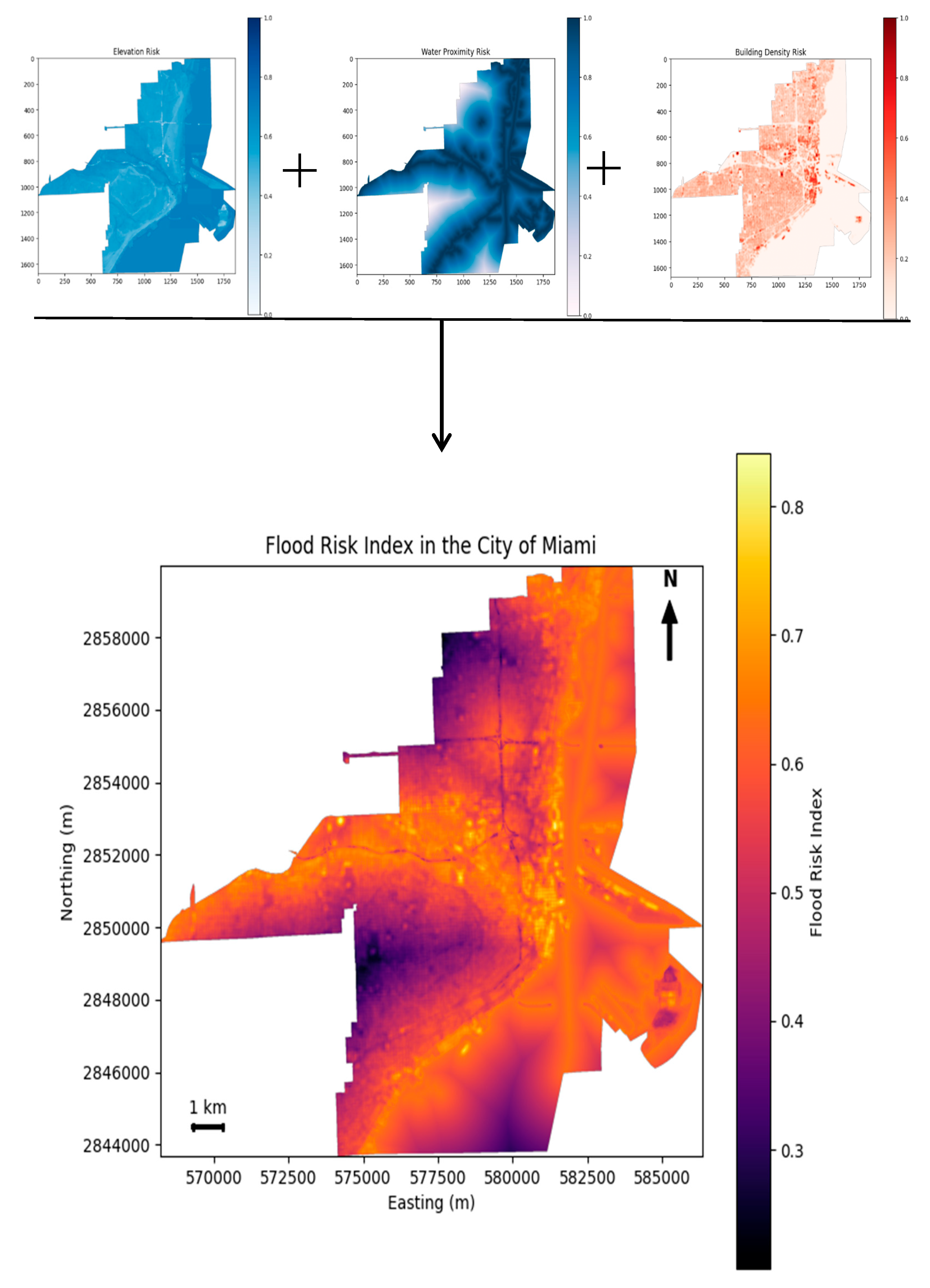
The three normalised risk indicators, elevation risk (elev_risk), water proximity risk (water_risk), and building density risk (density_n), were combined using a weighted linear overlay to produce a continuous composite flood risk index:
Risk = 0.40 × water_risk + 0.35 × elev_risk + 0.25 × density_n
The weight assignments reflect the theoretical priority ordering in coastal urban flood contexts: hydrological proximity is assigned the highest weight (0.40) consistent with literature consensus that distance to water is the dominant predictor of flood susceptibility [13,20]; terrain elevation receives the second-highest weight (0.35) reflecting gravitational controls on inundation; and building density receives a supplementary weight (0.25) capturing urban amplification effects. These weights sum to 1.0 and were applied without formal AHP consistency testing in the present study, a limitation discussed in Section 6.
The continuous risk index was classified into three susceptibility classes (low, medium, high) using quantile thresholds at the 33rd and 66th percentiles computed over valid (non-NaN) pixels within the study area. Quantile classification was selected over equal-interval or standard-deviation approaches to ensure an approximately equal distribution of study area pixels across classes, facilitating proportional comparison and reducing the influence of extreme value outliers on class boundaries [40].
4.7. Critical Facility Exposure Analysis
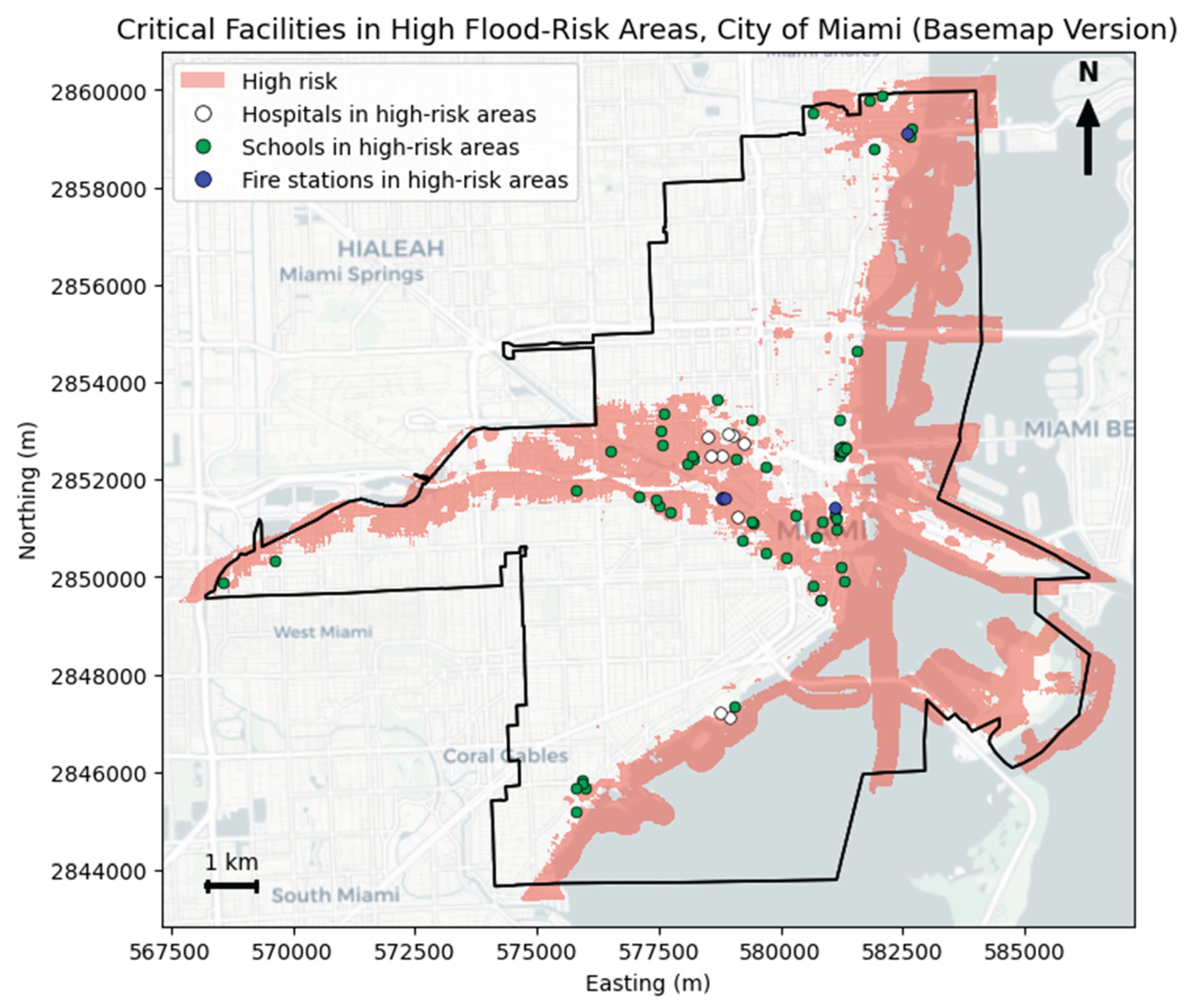
Hospitals, schools, and fire stations were extracted from OpenStreetMap using separate OSMnx queries with the tag dictionaries {‘amenity’: ‘hospital’}, {‘amenity’: ‘school’}, and {‘amenity’: ‘fire_station’} (with {‘emergency’: ‘fire_station’} as a fallback tag for legacy-tagged features). Retrieved polygon geometries were converted to representative point geometries using centroid calculation (to_point_geometry()), providing a consistent point-in-raster extraction basis. Risk class values were extracted at each facility point location from the classified risk raster using rasterio’s dataset indexing with the computed transform, yielding an integer class label (1 = low, 2 = medium, 3 = high) for each facility. Figure 7 shows the extracted critical facilities.
Facilities assigned class 3 were designated as high-risk and isolated for further reporting. Summary statistics were computed for each facility type: total count, high-risk count, and the proportion of each facility type located in the high-risk class. These proportional exposure indicators provide the primary metric for assessing differential vulnerability of healthcare, educational, and emergency service infrastructure to flood susceptibility.
Figure 8.
Flood Risk Index
5. Results
5.1. Flood Susceptibility Distribution
The continuous flood risk index exhibits clear spatial variation across the City of Miami, with high-risk values concentrated along the Biscayne Bay coastline, the Miami River corridor, and the dense network of drainage canals extending westward across the urban fabric. Lower risk values characterise the elevated ridgeline of the Miami Rock Ridge in the central and western portions of the city, corresponding to slightly higher terrain elevations and greater distance from major water bodies. Figure 9 shows low, medium, and high risks classification
Quantile classification at the 33rd and 66th percentile thresholds produces three susceptibility classes of approximately equal pixel count (Table 1). The low-susceptibility class covers 47.23 km2 (33.0% of study area), the medium-susceptibility class also covers 47.23 km2 (33.0%), and the high-susceptibility class covers 48.66 km2 (34.0%). The slight predominance of the high-risk class reflects the asymmetric distribution of the composite risk index, which is positively skewed by the extensive coastal and canal frontage areas that receive near-maximum water proximity risk values. The near-equal distribution across classes confirms that the quantile threshold selection provides reasonable discriminatory power across the study area.
5.2. Spatial Patterns of Flood Susceptibility
Spatially, the high-susceptibility class exhibits a distinctive coastal-corridor pattern. The highest risk values occur in a near-continuous band along the Biscayne Bay waterfront from Coconut Grove in the south through Brickell, Downtown, and Edgewater to Wynwood and Little Haiti in the north. Elevated susceptibility also extends inland along the principal drainage canal network, creating a west-east gradient of risk that reflects both water proximity and the relatively flat topography of the Miami coastal plain. Areas of consistently lower susceptibility correspond to the slight topographic elevation of the Overtown and Allapattah neighbourhoods where the Miami Rock Ridge provides 1–3 m of additional elevation above the coastal plain.
The spatial pattern of medium susceptibility occupies transition zones between the high-risk coastal and canal corridors and the lower-risk elevated interior. This zonal structure is broadly consistent with published FEMA flood insurance rate map boundaries for the City of Miami, in which Zone AE (100-year floodplain) and Zone VE (coastal high-hazard areas) concentrate along the same coastal and riverine corridors as the modelled high-susceptibility class.
5.3. Critical Facility Exposure
Exposure analysis reveals that a substantial proportion of critical facilities across all three categories are located within the high-susceptibility class (Table 2 & Figure 10). Hospitals exhibit the highest proportional exposure: 9 of 16 mapped hospital facilities (56.2%) are situated in high-susceptibility zones, representing a greater-than-expected proportion given that the high class covers only 34.0% of the study area (exposure ratio = 1.65). Schools show 25.0% exposure (61 of 244 facilities), slightly lower than the area-proportional expectation, suggesting partial correlation between school siting and neighbourhood-level flood risk variation. Fire stations exhibit 29.4% exposure (5 of 17 facilities), marginally below area-proportional expectation.
The disproportionate exposure of hospitals (exposure ratio = 1.65) is particularly noteworthy from a disaster risk perspective. Healthcare facilities are both especially critical during flood emergencies, serving simultaneously as treatment centres for flood-related injuries and as refuges for medically dependent populations, and are generally less replaceable in the short term than schools or fire stations, which have greater operational flexibility. This pattern echoes national findings by [10] and regional assessments by [25] identifying Miami-Dade hospitals as among the most flood-exposed healthcare assets in the southeastern United States.
Figure 11.
Exposure of critical facilities.
6. Discussion
6.1. Framework Performance and Spatial Validity
The cloud-native Python GIS framework presented in this study successfully generates a spatially coherent, interpretable flood susceptibility surface for the City of Miami that exhibits strong visual and qualitative agreement with established flood risk patterns documented in the existing literature. The high-susceptibility zones align with the coastal waterfront areas, Miami River corridor, and canal networks identified as primary flood exposure zones in FEMA flood insurance rate maps, Miami Beach’s Sea Level Rise Vulnerability Assessment (2024), and published hydraulic modelling studies of compound flooding in the city [7]. The hospital exposure finding (56.2% in high-susceptibility zones) aligns with [25] modelling-based assessment of Miami-Dade healthcare vulnerability and with [10] national coastal infrastructure risk analyses.
The framework’s three-factor MCDA design reflects a deliberate balance between simplicity, interpretability, and scientific defensibility. Water proximity, terrain elevation, and building density represent the three dominant physical controls on urban flood generation and exposure and are precisely the factors most consistently identified in GIS-MCDA flood susceptibility literature as high-importance indicators in coastal urban contexts ([13,14]. The use of uniform, data-driven normalisation (min-max scaling) ensures that all three indicators contribute across their full value ranges without artificial compression or expansion of distributions. The Euclidean distance transform approach for water proximity captures continuous spatial proximity more sensitively than binary buffer zones, while the uniform-filter approach for building density produces a smooth, noise-reduced proxy that more accurately represents neighbourhood-scale impervious surface patterns than raw pixel-level building presence.
The near-equal three-class distribution produced by quantile classification (33/33/34%) confirms that the chosen thresholds provide meaningful spatial discrimination rather than artificially concentrating risk estimates in a small geographic area. This is an important property for a decision-support tool intended to identify priority areas for further investigation: a susceptibility map that assigns 80% of the city to high risk provides little analytical leverage. The quantile approach thus ensures practical utility by providing a differentiated spatial risk signal across the full study area.
6.2. Transferability and Reproducibility
A key contribution of this framework is its demonstrated transferability: because all data sources are retrieved programmatically from publicly available APIs (USGS 3DEP via py3dep, OpenStreetMap via OSMnx), and all processing is implemented in open-source Python libraries executed in a cloud environment, the complete workflow can be re-applied to any US city by modifying a single geocoding string. Extension to international cities requires substitution of the DEM source (py3dep is US-specific; global alternatives include the NASADEM, COPERNICUS DEM, or SRTM retrieved via py3dep-compatible APIs) but all other components remain directly applicable. The OSMnx data retrieval functions are globally operational, and the GeoPandas/Rasterio/SciPy processing stack is entirely geography-agnostic.
This transferability has significant practical implications for flood risk governance. Many mid-size and lower-income coastal municipalities lack the resources for full hydraulic simulation campaigns but require spatial prioritisation tools to guide infrastructure investment, emergency preparedness planning, and zoning decisions. The cloud-native Python framework described here can be executed by a single analyst with basic Python literacy in Google Colaboratory within a few hours, providing a first-order susceptibility assessment that can directly inform planning processes. This aligns with the broader movement toward open, reproducible, and accessible geospatial science advocated by [15] [17], and [27].
6.3. Limitations
Several important limitations must be acknowledged. First, the framework produces a relative flood susceptibility index rather than an absolute flood hazard estimate in physical units. The composite risk index cannot be interpreted as flood depth, inundation probability, or return period frequency. It identifies areas that are more or less susceptible relative to the rest of the study area under the specified indicator weighting scheme, but does not quantify the physical flood mechanism or its statistical recurrence. For applications requiring quantitative risk thresholds, such as insurance underwriting, infrastructure design standards, or regulatory floodplain delineation; full hydraulic simulation models validated against observed flood events are required.
Second, the weighting scheme is partially subjective. While the weight assignments (0.40 / 0.35 / 0.25) are grounded in literature consensus and theoretical reasoning, they were applied without formal AHP pairwise comparison, consistency testing, or sensitivity analysis of alternative weight combinations. Different weight assignments could shift the spatial distribution of risk classes and alter the facility exposure proportions. Future extensions of this framework should include systematic sensitivity testing across plausible weight ranges and, where flood inventory data are available, calibration of weights against observed flood events using logistic regression or ROC curve optimisation ([20]).
Third, several relevant flood-conditioning factors were not incorporated due to data availability constraints within the open-source API ecosystem: soil permeability and infiltration capacity, stormwater drainage network capacity and condition, land cover beyond building footprints, groundwater depth, antecedent moisture conditions, and sea-level rise projections. The absence of a drainage infrastructure layer is a particularly significant omission for Miami, where the managed canal system plays a dominant role in stormwater conveyance and where infrastructure condition varies substantially across the city. Fourth, the centroid-based facility point extraction method simplifies large or irregular-footprint facilities to single points, potentially misclassifying facilities that span multiple risk classes.
Fifth, OSM data quality and completeness, while generally high in well-mapped cities like Miami [35], introduces uncertainty in facility inventories. Manual validation of the extracted hospital, school, and fire station datasets against authoritative municipal records would strengthen the exposure analysis. Some facilities may be absent from OSM or tagged with non-standard schemas, and the amenity taxonomy may not capture all relevant critical infrastructure categories.
6.4. Pathways for Enhancement
The framework can be enhanced through several tractable extensions. Validation against FEMA Flood Insurance Rate Maps, observed flood event records, or remote sensing-derived inundation extents would provide a quantitative assessment of classification accuracy and support weight calibration [14]. Integration of NLCD or Sentinel-2 derived land cover products would add an impervious surface fraction indicator that is physically more directly related to runoff generation than building density alone. Incorporation of LIDAR-derived void-filled DEMs at 1 m resolution, available for Miami-Dade through NOAA’s Digital Coast Programme; would substantially improve the elevation indicator’s sensitivity to the subtle microtopographic relief that governs local inundation patterns in such flat terrain. Future work should also extend the exposure analysis to additional critical infrastructure categories including water treatment plants, power substations, transportation hubs, and residential care facilities.
7. Conclusions
This paper has presented and evaluated a complete cloud-native Python GIS framework for flood susceptibility mapping and critical facility exposure analysis in Miami, Florida. The framework integrates three open-source spatial indicator; terrain elevation (10 m 3DEP DEM), Euclidean proximity to water bodies (OSM), and building footprint density (OSM), within a weighted MCDA overlay implemented in Google Colaboratory using Python geospatial libraries. The framework requires no proprietary software, no subscription data licences, and no local hardware beyond internet connectivity, making it immediately accessible and reproducible by any researcher or analyst.
Key findings demonstrate that high flood susceptibility covers 48.66 km2 (34.0%) of Miami, concentrated along coastal waterfronts, the Miami River corridor, and the drainage canal network. Hospitals exhibit the highest proportional exposure to high-susceptibility zones (56.2%; exposure ratio = 1.65), substantially exceeding the area-proportional expectation, while schools (25.0%) and fire stations (29.4%) show exposure levels near or below the area-proportional baseline. These findings highlight healthcare infrastructure as a priority target for detailed hydraulic analysis, climate adaptation planning, and emergency preparedness investment in Miami.
Methodologically, this study advances the case for open-source, cloud-native GIS as a viable and scientifically defensible platform for urban flood risk assessment, particularly in rapid screening and multi-city comparative applications where full hydraulic simulation is not practical. The framework’s single-parameter adaptability, requiring only a geocoding string change for application to other US cities, positions it as a transferable tool for the broader coastal urban risk governance community. Future work will extend the framework through integration of additional conditioning factors, validation against observed flood records, and sensitivity analysis of the weighting scheme.
References
- Tanoue, M.; Hirabayashi, Y.; Ikeuchi, H. Global-scale river flood vulnerability in the last 50 years. Sci. Rep. 2022, 6, 36021. [Google Scholar] [CrossRef]
- Wing, O. E. J.; Lehman, W.; Bates, P. D.; Sampson, C. C.; Quinn, N.; Smith, A. M.; Nardi, F. Inequitable patterns of US flood risk in the Anthropocene. Nat. Clim. Change 2022, 12, 156–162. [Google Scholar] [CrossRef]
- IPCC. Climate Change 2022: Impacts, Adaptation and Vulnerability. Contribution of Working Group II to the Sixth Assessment Report; Cambridge University Press, 2022. [Google Scholar] [CrossRef]
- Kulp, S. A.; Strauss, B. H. New elevation data triple estimates of global vulnerability to sea-level rise and coastal flooding. Nat. Commun. 2019, 10, 4844. [Google Scholar] [CrossRef]
- Jongman, B.; Winsemius, H. C.; Fraser, S. A.; Muis, S.; Ward, P. J. Assessment and adaptation to climate change–related flood risks. In Oxford Research Encyclopedia of Natural Hazard Science; 2021. [Google Scholar]
- Rentschler, J.; Salhab, M.; Jafino, B. A. Flood exposure and poverty in 188 countries. Nat. Commun. 2022, 13, 3527. [Google Scholar] [CrossRef]
- Peña, F.; Obeysekera, J.; Jane, R.; Nardi, F.; Maran, C.; Cadogan, A.; de Groen, F.; Melesse, A. Investigating compound flooding in a low elevation coastal karst environment using multivariate statistical and 2D hydrodynamic modeling. Weather Clim. Extrem. 2023, 39, 100534. [Google Scholar] [CrossRef]
- Li, C.; Xue, Y.; Fu, X. Urban built environment and flood ramifications: Evidence from insurance claims data in Miami, Florida. J. Am. Plan. Assoc. 2026. [Google Scholar] [CrossRef]
- Hallegatte, S.; Green, C.; Nicholls, R. J.; Corfee-Morlot, J. Future flood losses in major coastal cities. Nat. Clim. Change 2013, 3, 802–806. [Google Scholar] [CrossRef]
- Union of Concerned Scientists. Underwater: Rising seas, chronic floods, and the implications for US coastal real estate; UCS Publications, 2024; Available online: https://www.ucsusa.org/resources/underwater.
- Teng, J.; Jakeman, A. J.; Vaze, J.; Croke, B. F. W.; Dutta, D.; Kim, S. Flood inundation modelling: A review of methods, recent advances and uncertainty analysis. Environ. Model. Softw. 2017, 90, 201–216. [Google Scholar] [CrossRef]
- Leandro, J.; Schumann, A.; Pfister, A. A step towards considering the spatial heterogeneity of urban key features in urban hydrology flood modelling. J. Hydrol. 2021, 445, 1–13. [Google Scholar] [CrossRef]
- Kaya, C. M.; Derin, L. Parameters and methods used in flood susceptibility mapping: A review. J. Water Clim. Change 2023, 14, 1935–1960. [Google Scholar] [CrossRef]
- Nguyen, H. N.; Fukuda, H.; Nguyen, M. N. Assessment of the susceptibility of urban flooding using GIS with an analytical hierarchy process in Hanoi, Vietnam. Sustainability 2024, 16, 3934. [Google Scholar] [CrossRef]
- Boeing, G. OSMnx: New methods for acquiring, constructing, analyzing, and visualizing complex street networks. Comput. Environ. Urban Syst. 2017, 65, 126–139. [Google Scholar] [CrossRef]
- Gillies, S.; van der Wel, C.; Van den Bossche, J.; Taves, M. W.; Arnott, J.; Ward, B. C.; others. Rasterio: Geospatial raster I/O for Python programmers. GitHub. 2019. Available online: https://github.com/rasterio/rasterio.
- Snow, A. D.; Scott, R.; Raspaud, M.; Kousoulas, J.; others. rioxarray: Geospatial capabilities for xarray; Zenodo, 2022. [Google Scholar] [CrossRef]
- Head, T.; Kumar, M.; Claesen, M.; Jalali, A.; others. scikit-optimize: Sequential model-based optimization library. 2019. [Google Scholar] [CrossRef]
- Tehrany, M. S.; Pradhan, B.; Mansor, S.; Ahmad, N. Flood susceptibility assessment using GIS-based support vector machine model with different kernel types. Catena 2014, 125, 91–101. [Google Scholar] [CrossRef]
- Malczewski, J. GIS-based multicriteria decision analysis: A survey of the literature. Int. J. Geogr. Inf. Sci. 2006, 20, 703–726. [Google Scholar] [CrossRef]
- Tehrany, M. S.; Kumar, L.; Shabani, F. A new GIS-based data mining technique using an adaptive neuro-fuzzy inference system (ANFIS) and k-fold cross-validation approach for land susceptibility mapping. Nat. Hazards 2022, 110, 1–25. [Google Scholar]
- Shahabi, H.; Shirzadi, A.; Ghaderi, K.; Omidvar, E.; Al-Ansari, N.; Clague, J. J. Flood detection and susceptibility mapping using Sentinel-1 SAR and machine learning approaches in a coastal watershed of Iran. In Remote Sensing; Mosavi, A., Ed.; 2024; Volume 12. [Google Scholar] [CrossRef]
- Zahura, F. T.; Goodall, J. L. Predicting combined tidal and pluvial flood inundation using a machine learning surrogate model. J. Hydrol. Reg. Stud. 2022, 41, 101087. [Google Scholar] [CrossRef]
- Xu, H.; Ma, C.; Lian, J.; Xu, K.; Chaima, E. Urban flooding risk assessment based on an integrated k-means cluster algorithm and improved entropy weight method in the context of urban sprawl. J. Hydrol. 2020, 571, 11–20. [Google Scholar] [CrossRef]
- Shen, Y.; Morsy, M. M.; Huxley, C.; Tahvildari, N.; Goodall, J. L. Flood risk assessment and increased resilience for coastal urban watersheds under the combined impact of storm tide and heavy rainfall. J. Hydrol. 2021, 569, 428–442. [Google Scholar] [CrossRef]
- Kelsey, J.; Gillies, S.; others. GeoPandas: Python geospatial data library. GitHub. 2020. Available online: https://github.com/geopandas/geopandas.
- Chegini, T.; Li, H.-Y.; Leung, L. R. HyRiver: Hydroclimate data retriever. J. Open Source Softw. 2021, 6, 3175. [Google Scholar] [CrossRef]
- Odum, P. Democratising Spatial Intelligence: Achieving Efficiency with Less, while Flattening the Learning Curve with AI-Assisted Python in the Cloud; 2026. [Google Scholar]
- Moradi, M.; Roche, S.; Mostafavi, M. A. Evaluating OSM building footprint data quality in Québec Province, Canada from 2018 to 2023. Geomatics 2023, 3, 541–562. [Google Scholar] [CrossRef]
- Van den Hoek, J.; Friedrich, H. K.; Ballasiotes, A.; Peters, L. E. R.; Wrathall, D. Development after displacement: Evaluating the utility of OpenStreetMap data for monitoring Rohingya refugee settlement. Geosciences 2022, 11, 151. [Google Scholar] [CrossRef]
- Barnard, P. L.; Erikson, L. H.; Foxgrover, A. C.; Hart, J. A. F.; Limber, P.; O’Neill, A. C.; Wood, N. J. Dynamic flood modeling essential to assess the coastal impacts of climate change. Sci. Rep. 2021, 9, 4309. [Google Scholar] [CrossRef] [PubMed]
- Deri, F.; Mara, F.; Anselmi, C.; Chioni, C. Crowdsourced data for urban planning: A critical evaluation of OpenStreetMap accuracy and completeness. In Lecture Notes in Computer Science; Springer, 2026; Vol. 15897. [Google Scholar] [CrossRef]
- OpenStreetMap Wiki Stats. 2024. Available online: https://wiki.openstreetmap.org/wiki/Stats.
- Haklay, M. How good is volunteered geographical information? A comparative study of OpenStreetMap and Ordnance Survey datasets. Environ. Plan. B Plan. Des. 2010, 37, 682–703. [Google Scholar] [CrossRef]
- Biljecki, F.; Chow, Y. S.; Lee, K. Quality of crowdsourced geospatial building information: A global assessment of OpenStreetMap attributes. Build. Environ. 2023, 237, 110295. [Google Scholar] [CrossRef]
- Komi, K.; Neal, J.; Trigg, M. A.; Diekkrüger, B. Modelling of flood hazard extent in data scarce areas: A case study of the Oti River basin, West Africa. J. Hydrol. Reg. Stud. 2021, 10, 122–132. [Google Scholar] [CrossRef]
- Judah, A.; Hu, B. The integration of optical and SAR data for identifying flood damage and flash flood susceptibility using machine learning approaches. Remote Sens. 2021, 13, 2989. [Google Scholar] [CrossRef]
- Cutter, S. L.; Ash, K. D.; Emrich, C. T. The geographies of community disaster resilience. Glob. Environ. Change 2020, 50, 65–77. [Google Scholar] [CrossRef]
- Junger, A.; Reuss, J.; Yohannes, E. Long-term community impacts of flood events on school and educational infrastructure. Int. J. Disaster Risk Reduct. 2021, 55, 102078. [Google Scholar] [CrossRef]
- Jenks, G. F.; Caspall, F. C. Error on choroplethic maps: Definition, measurement, reduction. Ann. Am. Assoc. Geogr. 1971, 61, 217–244. [Google Scholar] [CrossRef]
Figure 1.
Study location.
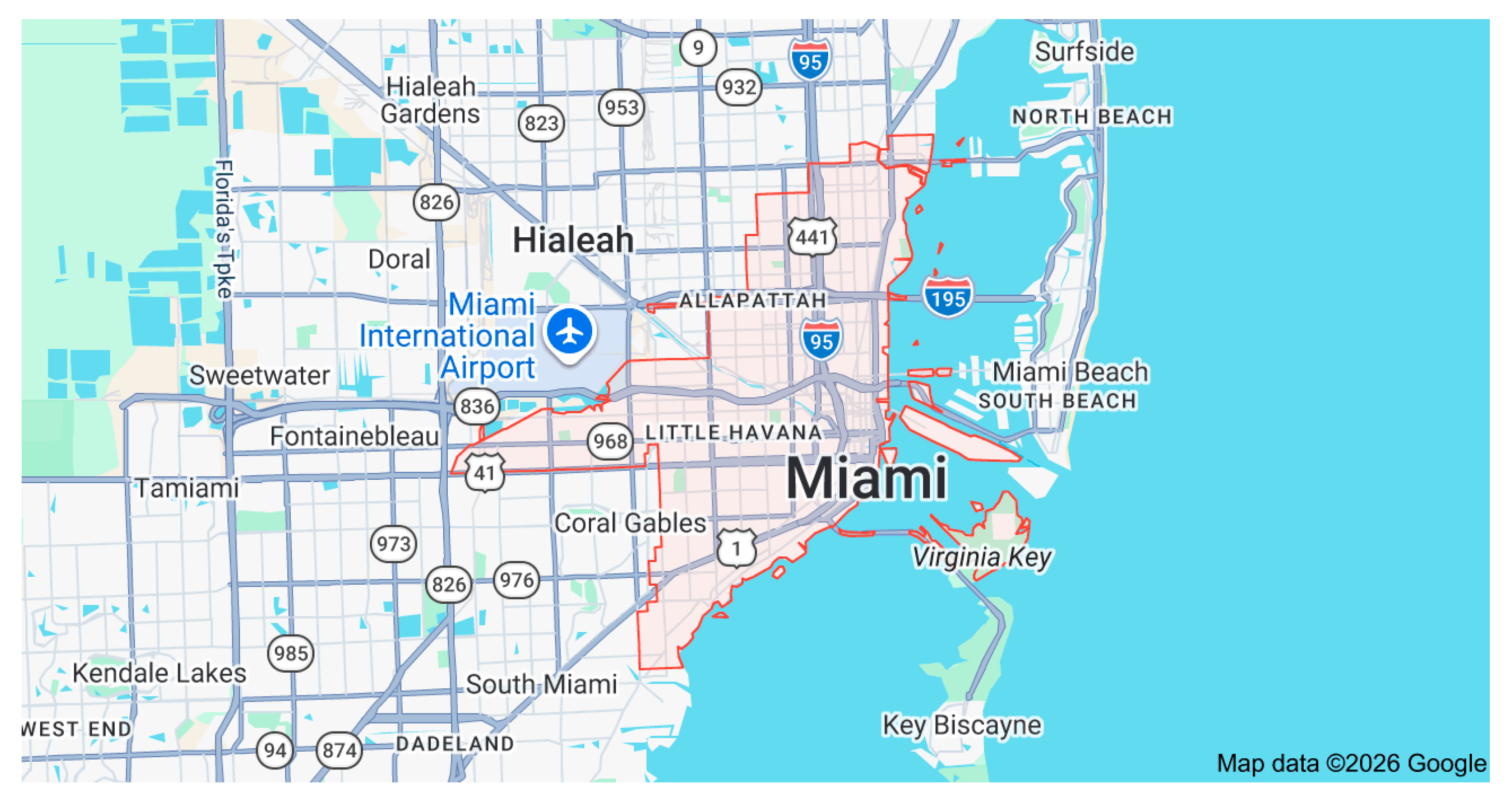
Figure 2.
Workflow Chart.
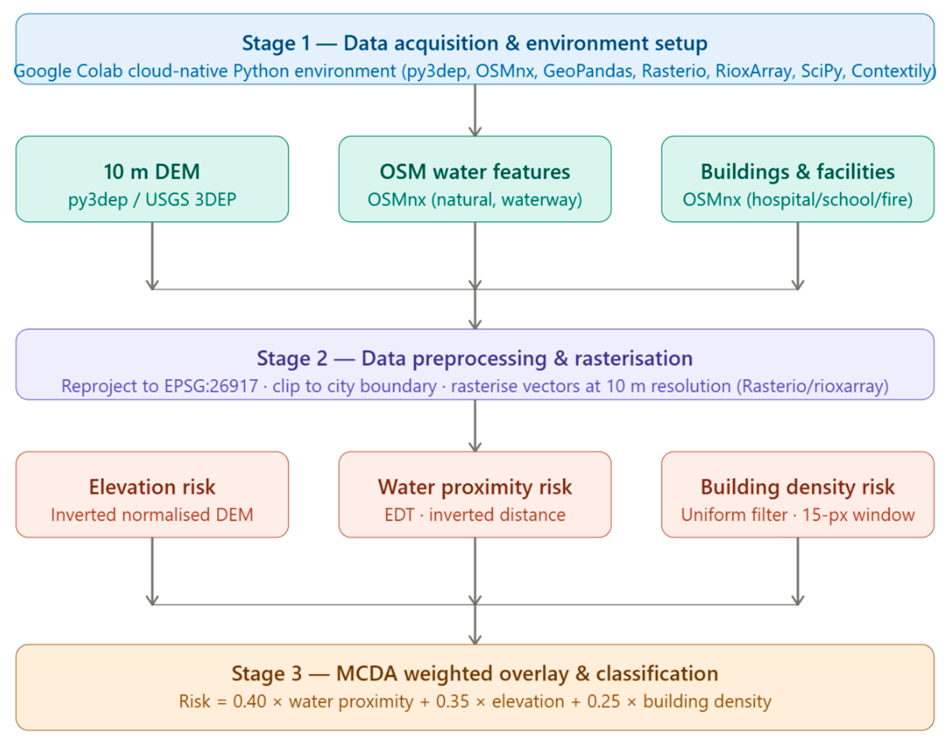
Figure 3.
Clipped DEM.
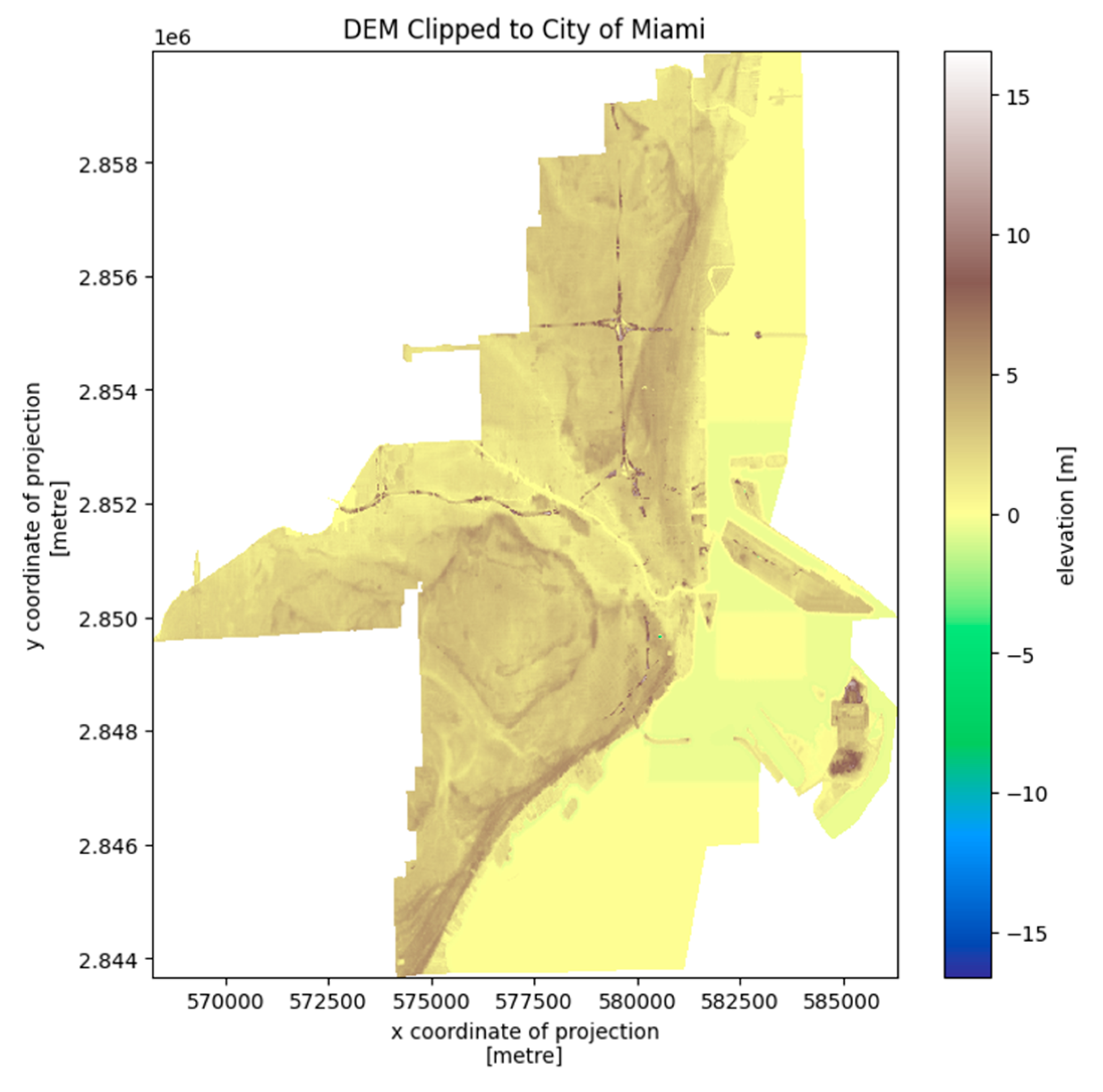
Figure 4.
Extracted Water Feature.
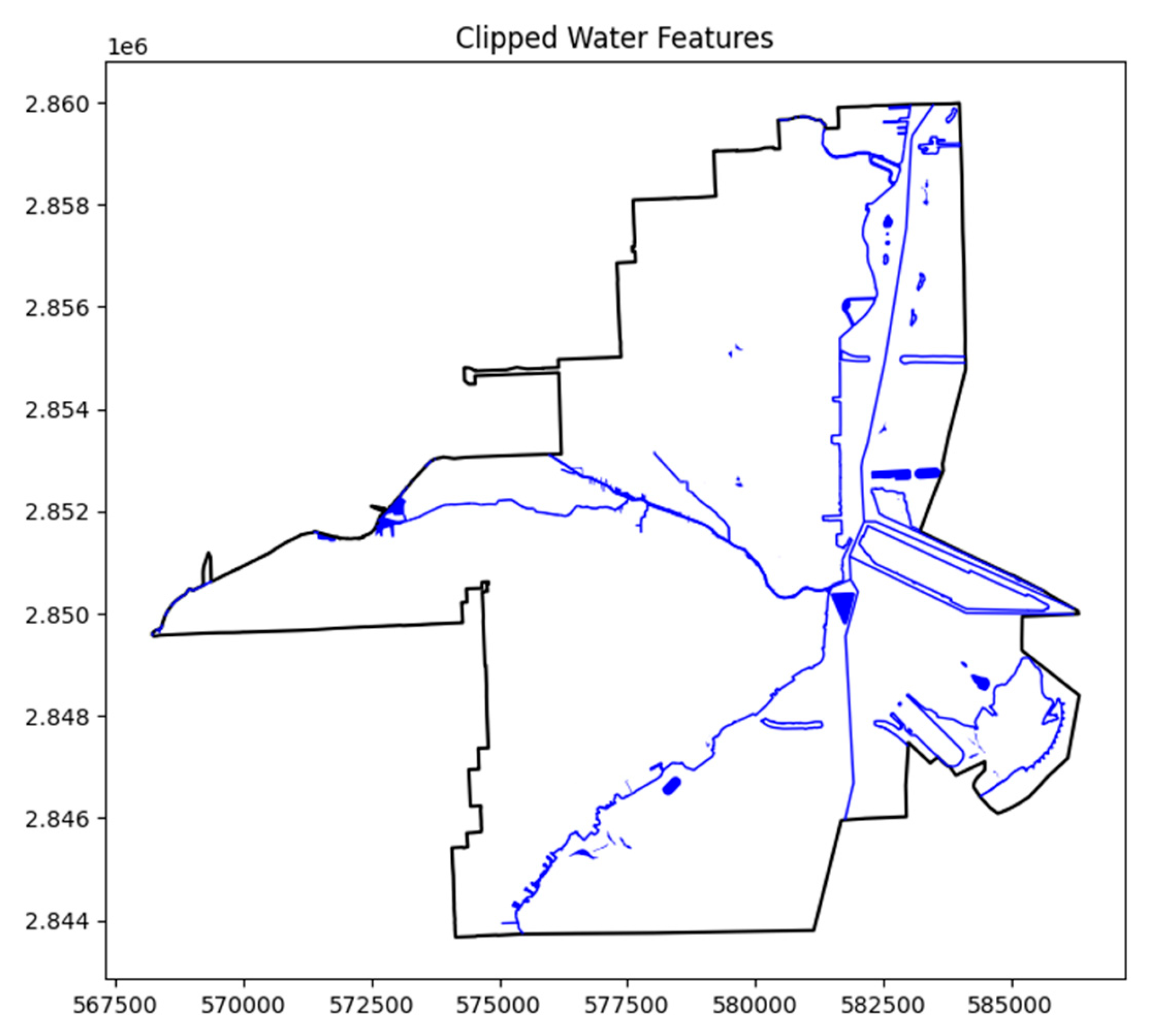
Figure 5.
Rasterised Water Feature.
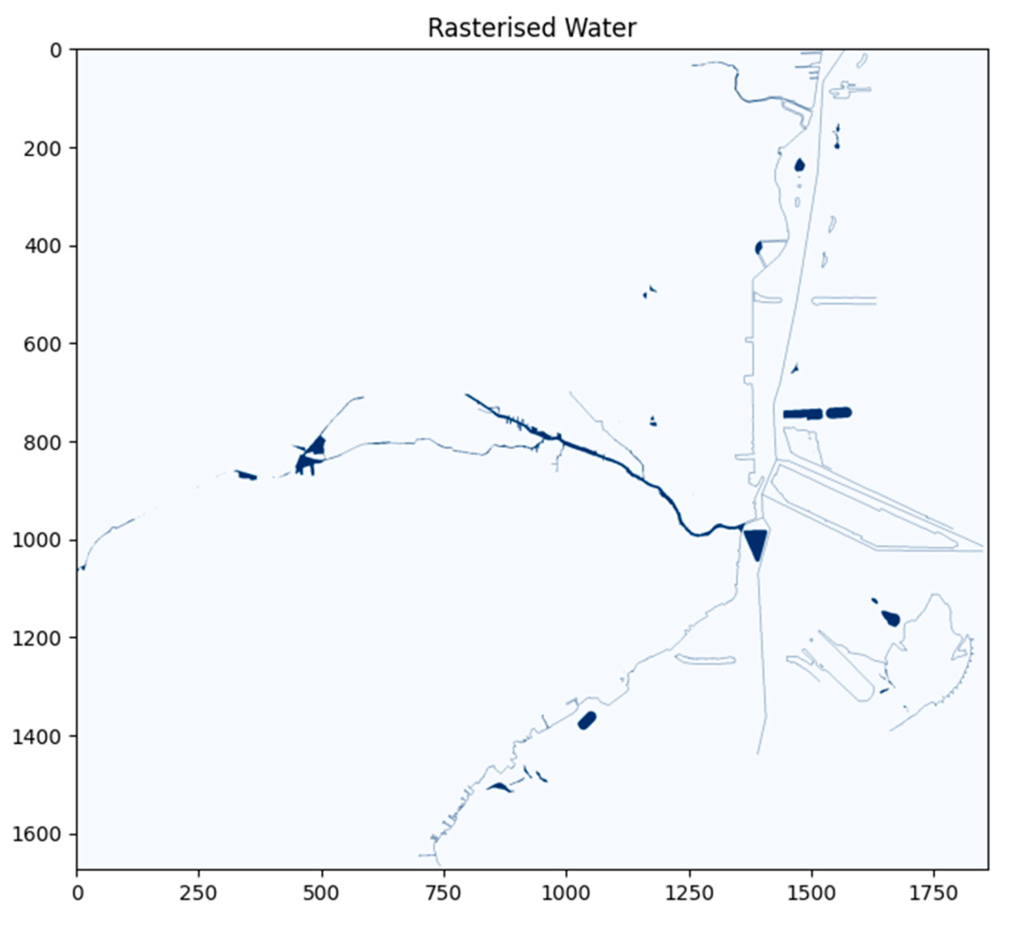
Figure 6.
Rasterised Building features
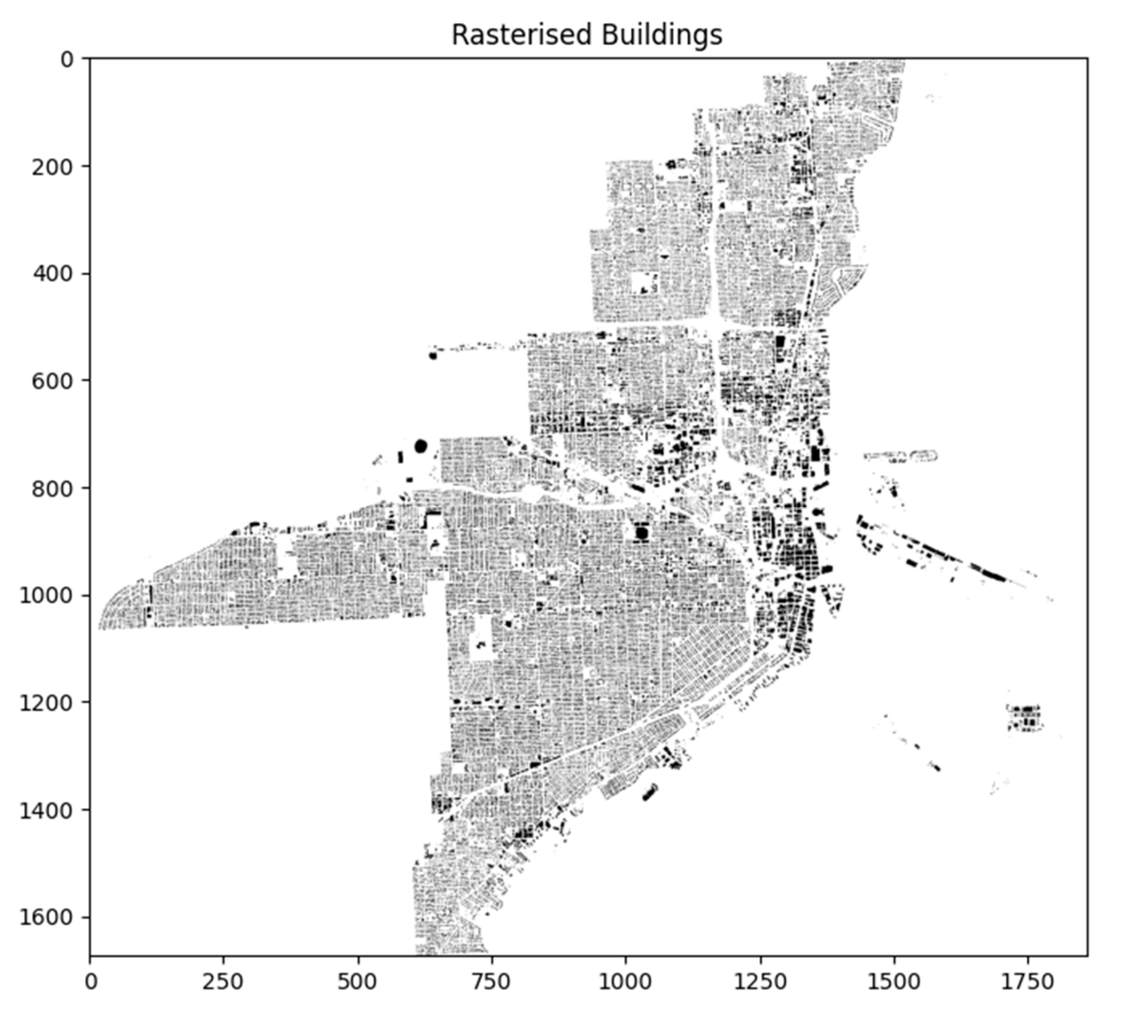
Figure 7.
Extracted Critical Facilities.
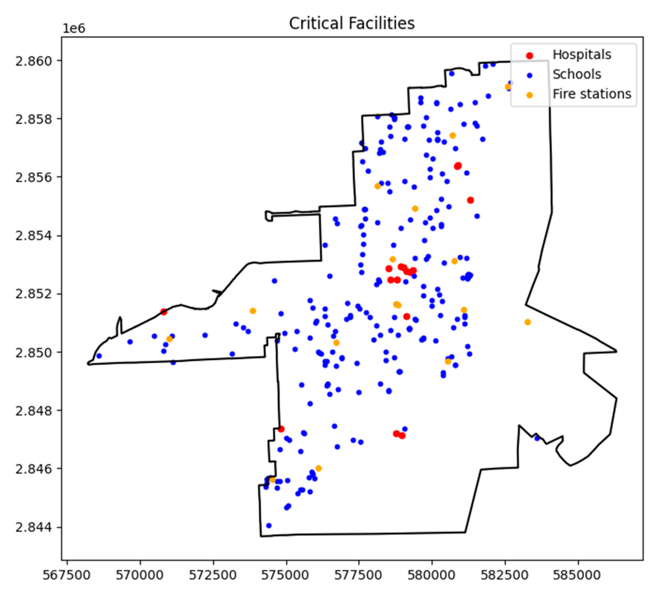
Figure 9.
Flood Risk Classification.
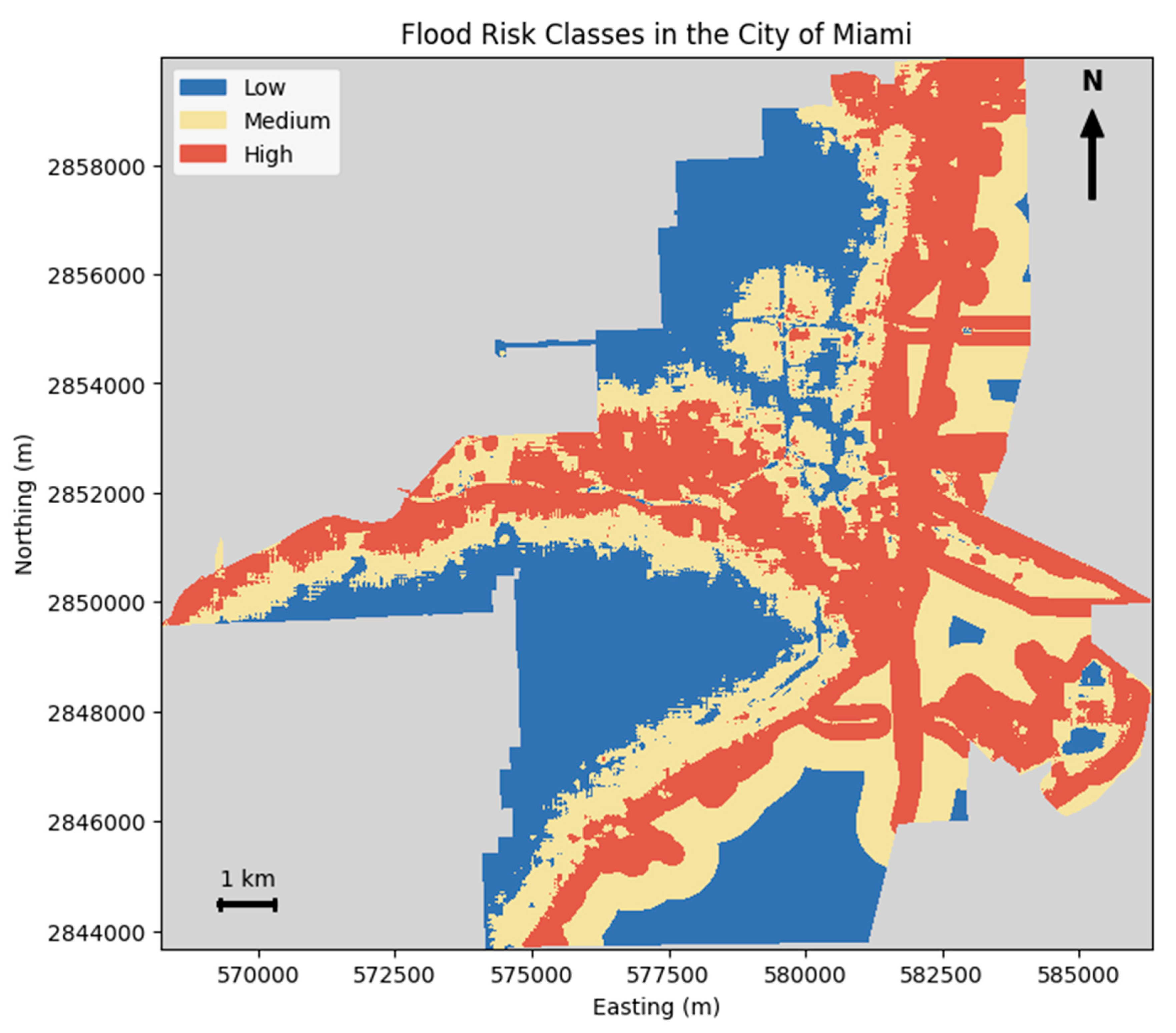
Figure 10.
Critical Facilities in High-Risk Areas.
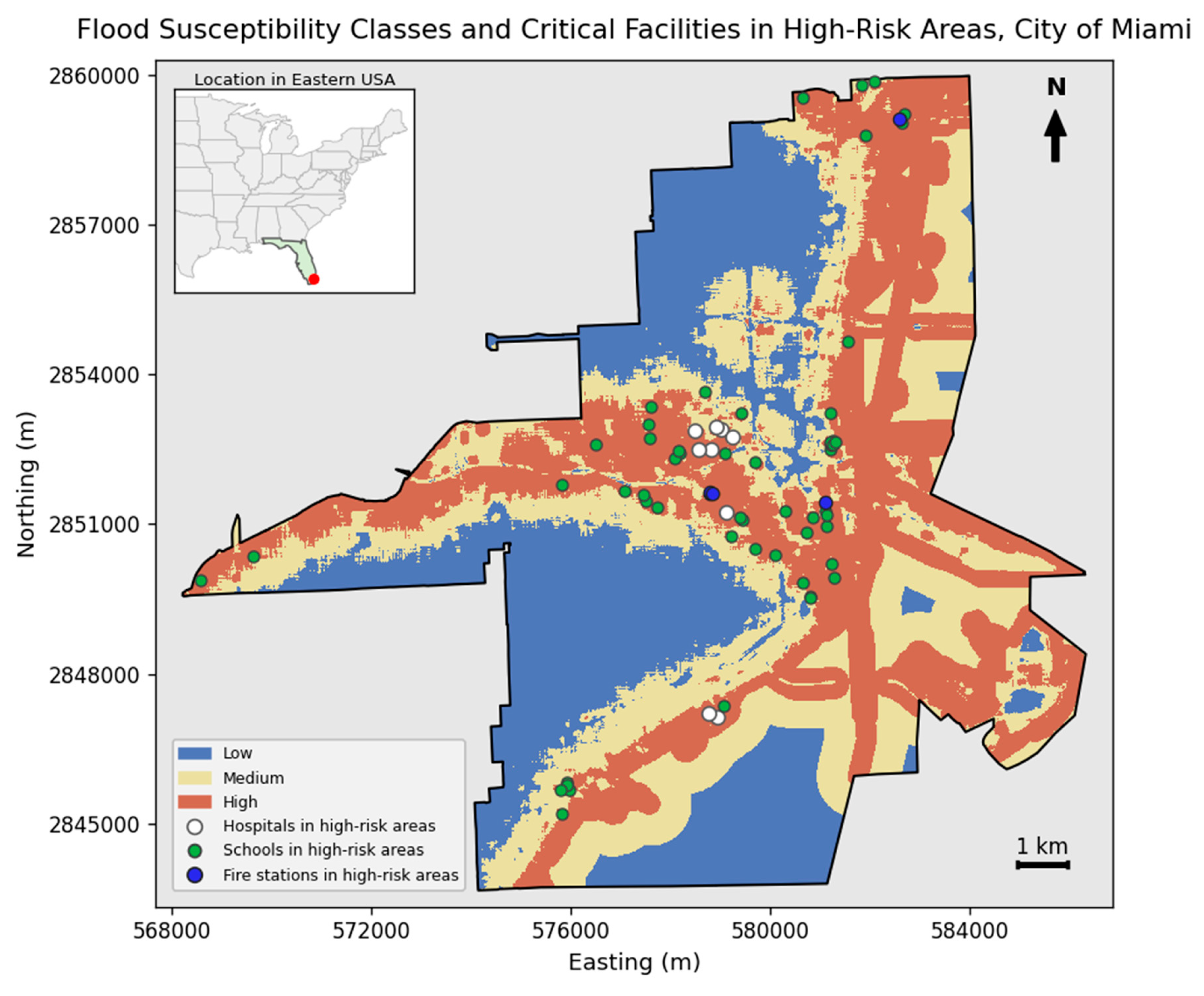

Table 1.
Flood susceptibility class distribution across the City of Miami.
| Susceptibility class | Pixel count | Area (km2) | % of study area | Index range |
|---|---|---|---|---|
| Low | 472,260 | 47.23 | 33.0 | 0–q1 |
| Medium | 472,260 | 47.23 | 33.0 | q1–q2 |
| High | 486,570 | 48.66 | 34.0 | >q2 |
| Total | 1,431,090 | 143.12 | 100.0 | — |
Note: q1 = 33rd percentile threshold; q2 = 66th percentile threshold. Pixel area = 100 m2 (10 m × 10 m resolution).
Table 2.
Critical facility exposure by flood susceptibility class.
| Facility type | Total | Low risk | Medium risk | High risk | High risk (%) | Exposure ratio |
|---|---|---|---|---|---|---|
| Hospitals | 16 | 4 | 3 | 9 | 56.2% | 1.65 |
| Schools | 244 | 88 | 95 | 61 | 25.0% | 0.74 |
| Fire stations | 17 | 7 | 5 | 5 | 29.4% | 0.87 |
Note: Exposure ratio = (high-risk facility % / high-risk area %). Values >1.0 indicate greater-than-area-proportional exposure.
Disclaimer/Publisher’s Note: The statements, opinions and data contained in all publications are solely those of the individual author(s) and contributor(s) and not of MDPI and/or the editor(s). MDPI and/or the editor(s) disclaim responsibility for any injury to people or property resulting from any ideas, methods, instructions or products referred to in the content. |
© 2026 by the authors. Licensee MDPI, Basel, Switzerland. This article is an open access article distributed under the terms and conditions of the Creative Commons Attribution (CC BY) license (http://creativecommons.org/licenses/by/4.0/).
Copyright: This open access article is published under a Creative Commons CC BY 4.0 license, which permit the free download, distribution, and reuse, provided that the author and preprint are cited in any reuse.