

Submitted:
07 May 2026
Posted:
08 May 2026
You are already at the latest version
Abstract
Rapid detection and localization of liquid fuel spills is critical for first responders assessing fire and health hazards, yet current methods require ground-based sampling or specialized instrumentation, limiting their practicality for wide-area emergency response. We present a drone-based passive colorimetric sensor system using test strips impregnated with Nile red, similar to colored confetti. Nile red is a solvatochromic dye that undergoes distinct visible color transitions upon exposure to different liquids. The dye is embedded within a polymer matrix that minimizes leaching while providing high optical contrast between dry, water-exposed, and fuel-exposed states. The sensor strips exhibit solvent-specific colorimetric responses within one minute of exposure, readily detectable by standard RGB cameras mounted on unmanned aerial vehicles (UAV) at altitudes up to 50 m. Automated classification was validated at 20 m altitude, enabling remote surveillance of contaminated surfaces without specialized equipment. Color-corrected image analysis using Calibrite ColorChecker calibration ensures reliable interpretation under variable field illumination (625–77,000 lux). Systematic laboratory evaluation of twelve fossil and bio-derived fuels revealed characteristic hue shifts that clearly discriminate ethanol-containing gasoline blends from diesel-range fuels. Field validation confirmed localization and classification of fuel-exposed sensors, achieving F1 scores of 0.94 for gasoline and 0.98 for diesel detection with no false positives in the tested scenarios. This cost-effective and scalable approach provides actionable information on both contamination location and fuel type, crucial for rapid hazard assessment in emergency response scenarios.
Keywords:
UAV
; Nile red
; first responders
; chemical accident
; hazard assessment
; HAZMAT
; hue analysis
; cellulose test strip
; aerial surveillance
; environmental monitoring
1. Introduction
Contamination with liquid fuels poses a persistent and very common threat to environmental integrity and public health. Accidental spills, storage tank failures, and transportation accidents can cause fire hazards and extensive soil and groundwater contamination [1,2]. Acute exposure to gasoline and diesel vapors causes airway irritation and, upon aspiration, chemical pneumonitis. Chronic exposure to aromatic components, particularly benzene, is hematotoxic and increases leukemia risk [3,4]. The urgency of rapid detection is particularly high for large-scale or remote contamination sites, where immediate hazard assessment is essential to minimize health, environmental impacts, and particularly fire or explosion hazards.
Unmanned aerial vehicles (UAV) have expanded the possibilities for environmental monitoring and enable safe surveillance of hazardous areas that pose risks to ground personnel [5,6,7,8,9,10]. However, current airborne chemical sensing approaches face fundamental constraints. Drone-mounted gas sensors suffer from aerodynamic interference, as rotor downwash disrupts sampling accuracy and disperses volatile analytes [11,12,13]. Advanced remote-sensing modalities such as hyperspectral imaging or laser-induced fluorescence show good sensitivity but very limited chemical information, require complex instrumentation at often prohibitively high costs, limiting routine deployment [14,15,16]. Physical sample collection from UAV platforms remains logistically challenging. These limitations highlight the need for lightweight, passive sensing approaches that decouple chemical detection from the aerodynamic and payload constraints of multi-rotor platforms [17].
Conventional detection methods such as gas chromatography–mass spectrometry (GC-MS) and infrared spectroscopy (IR) provide high analytical precision but require expensive instrumentation, extensive sample preparation, and trained personnel, reducing their applicability in field scenarios [18]. Portable colorimetric sensors have emerged as a complementary approach, offering field-deployable operation with low complexity [19,20]. Among chromophores suitable for liquid detection, solvatochromic dyes are especially promising because their optical properties shift significantly with solvent polarity [21,22,23]. Nile red, a benzophenoxazine dye, is a prominent example, exhibiting pronounced color transitions between polar and nonpolar environments [24,25]. While prior studies have mainly exploited fluorescence, these approaches require controlled illumination and sophisticated optics. In contrast, the visible absorption-based color change of Nile red can be captured with standard RGB cameras, eliminating the need for specialized optics or excitation sources.
This feature is particularly attractive for UAV-based remote sensing, where lightweight, low-complexity optical payloads are advantageous. More broadly, camera-readable colorimetric responses enable distributed sensing strategies in which the chemical recognition element remains passive, while information is acquired remotely by an aerial imaging platform. Building upon the “Passive Smart Dust” concept introduced in our previous work, we extend this framework from pH-based acid/base detection [26] to the classification of liquid fuel contamination. In the Passive Smart Dust approach, small, low-cost sensor papers, like confetti snippets, operate without any electronics or internal power supply. Instead, they use intrinsic material properties, e.g. solvatochromism, to provide information that can be accessed remotely via optical imaging from a UAV platform. This transition presents an additional challenge: While pH-sensitive indicators produce strong, clear color changes, the solvatochromic response to fuels results in more subtle color changes that require a robust sensor formulation and calibrated image analysis to ensure reliable classification under variable field conditions.
The main contributions of this work are: (I) Development of a Nile red paper sensor that appears white when dry and undergoes a pronounced color change upon contact with liquid fuels. (II) Systematic evaluation of solvatochromic hue signatures across twelve fuel types, enabling differentiation of ethanol-containing gasoline blends from diesel-type fuels. (III) A standardized ColorChecker-based calibration protocol for consistent color quantification across laboratory and field illumination conditions (625–77,000 lux). (IV) UAV field validation with an automated image processing pipeline for detecting and geolocating fuel spills from an altitude of 20 meters.
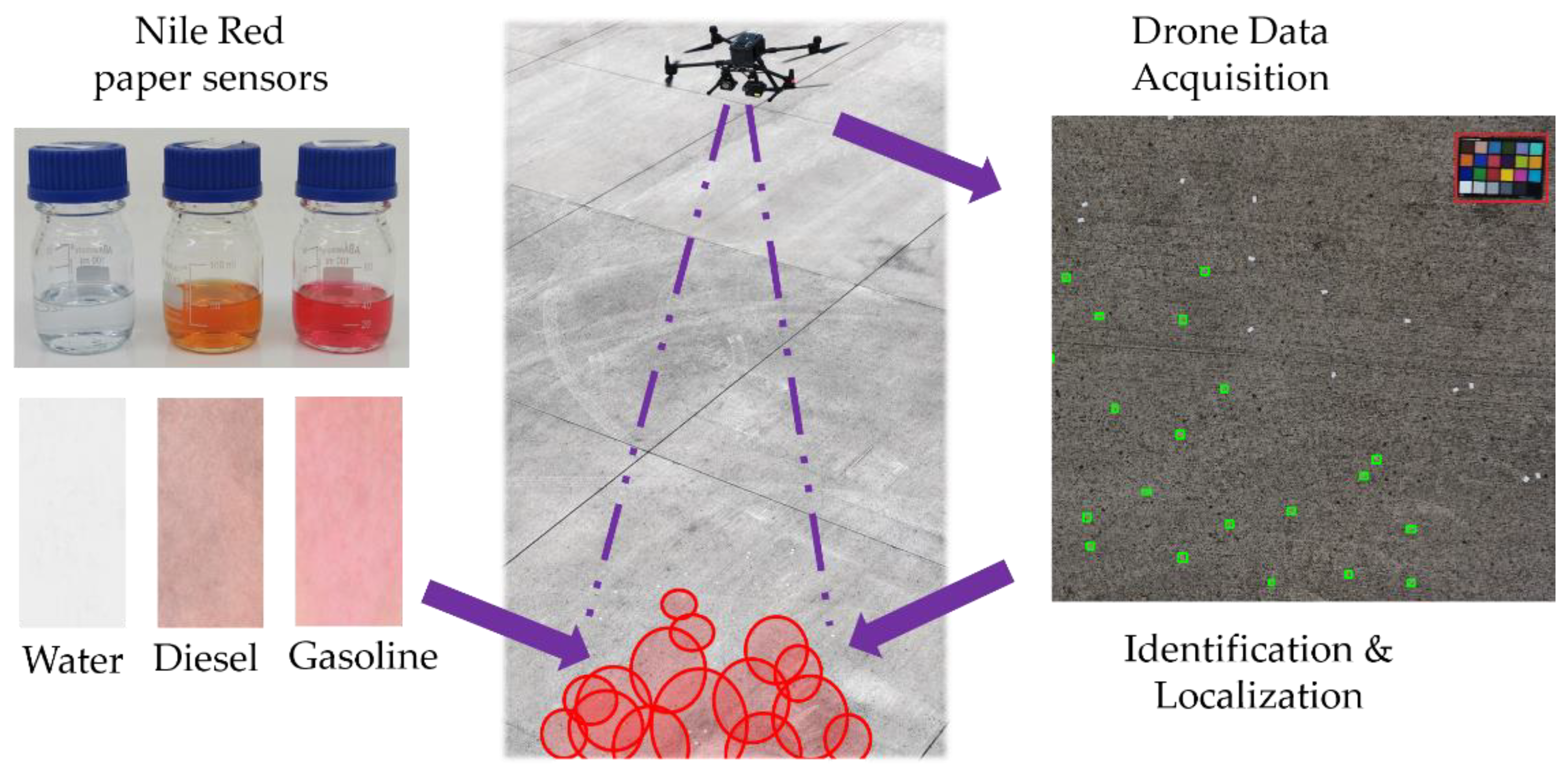
Figure 1.
Graphical abstract of the Passive Smart Dust concept. Colorimetric paper-based test strips with Nile red embedded in a polymer respond specifically to different liquid fuels (left). The test strips were deployed in the field, and their colorimetric response was recorded by a UAV at 20-meter altitude (middle). Potential contamination sites were identified and geolocated using a custom image processing algorithm. (right).
Figure 1.
Graphical abstract of the Passive Smart Dust concept. Colorimetric paper-based test strips with Nile red embedded in a polymer respond specifically to different liquid fuels (left). The test strips were deployed in the field, and their colorimetric response was recorded by a UAV at 20-meter altitude (middle). Potential contamination sites were identified and geolocated using a custom image processing algorithm. (right).
Nile red (9-diethylamino-5H-benzo[α]phenoxazin-5-one) is a lipophilic benzophenoxazine dye with pronounced solvatochromic properties arising from intramolecular charge transfer (ICT) between the diethylamino donor and phenoxazinone acceptor moieties [27]. Upon photoexcitation, the dipole moment increases by approximately 1.8 D relative to the ground state, with the HOMO localized primarily on the donor group and the LUMO on the acceptor core. In polar solvents, stabilization of the ICT state leads to bathochromic shifts in both absorption and emission spectra, whereas nonpolar environments induce hypsochromic shifts, producing a distinctive, blue-shifted colorimetric response exploitable for solvent detection [28,29].
In aqueous media, Nile red exhibits poor solubility and forms non-emissive H-type aggregates via π–π stacking, resulting in blue-shifted absorption and quenched fluorescence [25,30]. Hydrogen bonding with protic solvents further reduces quantum yield and lifetime through nonradiative decay. In contrast, in nonpolar hydrocarbons and short-chain alkanols, Nile red shows intense emission, with red shifts increasing with solvent polarity and hydrogen-bonding capacity; longer-chain alcohols tend to promote aggregation and diminish spectral shifts [31].
These pronounced polarity-dependent spectral changes enable selective sensing of nonpolar hydrocarbons against aqueous backgrounds as seen in Figure 2 [32]. The dye maintains stable optical properties in fuels such as gasoline, kerosene, and isooctane, with minimal degradation during thermo-oxidative aging and demonstrated antioxidant activity. Spectral shifts in fuel–ethanol blends correlate with ethanol content, and emission intensity decreases with increasing temperature, providing temperature-dependent sensing capability [33,34]. Other solvents not belonging to fuels were also tested (supplement Figures S6, S8). The incorporation into polymer matrices preserves the solvatochromic reaction while delaying the leaching of the dye, enabling robust solid-state sensors [35]. In such matrices, emission maxima shift according to the local dielectric constant, and multiexponential fluorescence decays reflect coexisting locally excited and ICT states. This environmental sensitivity, combined with stability in hydrocarbon-based media, underpins Nile red’s suitability as a functional dye for polymer-based colorimetric fuel detection.
2. Materials and Methods
2.1. Preparation of Test Strips
Filter paper (MN 617, Macherey-Nagel, Düren, Germany), composed of pure cellulose, was selected as the base substrate for sensor fabrication. The paper was pretreated by immersion in 0.1 M sodium hydroxide solution (Honeywell, Raunheim, Germany) for 10 s, followed by thorough rinsing with ultrapure water to remove residual alkali. A polymer coating solution was prepared by slowly adding 250 mg of poly(acrylic acid sodium salt) (PAA-Na, Mw ≈ 2,100 g mol⁻¹, CAS 9003-04-7, Sigma-Aldrich, Merck KGaA, Darmstadt, Germany) and 125 mg of poly(vinyl alcohol) (PVA, 87–90% hydrolyzed, Mw 30,000–70,000 g mol⁻¹, CAS 9002-89-5, Merck KGaA, Darmstadt, Germany) to 40 mL of ultrapure water under constant stirring at 60 °C for 30 min. After cooling to room temperature, 4 mg of Nile red (Carl Roth, Karlsruhe, Germany; CAS 7385-67-3) was added. The mixture was homogenized with a high-power ultrasonic disperser (Hielscher UP200St, Sonotrode S26d2) at 100% amplitude for 12 min, followed by ultrasonic treatment in a bath sonicator (Elma TI-H-5, 45 kHz) for an additional 10 min to ensure uniform dye distribution. Excess non-suspended dye was removed from the emulsion by filtration, using a Whatman® PTFE syringe filter with 0.2 µm pore size.
The dye–polymer suspension was applied to the pretreated paper by dip-coating for 20 s. Coated papers were dried overnight by placing them in a laboratory fume hood at room temperature (Figure 3). After drying, the test strips were cut into pieces of 1 × 2 cm and stored in sealed containers at 4 °C until use. The resulting test strips appeared white under ambient light and exhibited distinct color changes upon contact with liquid fuels and other solvents. The strips were designed to provide reliable colorimetric responses under outdoor deployment and UAV imaging conditions.
2.2. Calibration and Color Correction
A comprehensive laboratory calibration protocol was implemented to establish optimal colorimetric accuracy for color hue determination. Images were acquired using a Pentax K10D digital SLR camera (Pentax Corporation, Tokyo, Japan) with a 10.2 MP APS-C CCD sensor (23.5 × 15.7 mm) and an SMC-DA 18-55 mm f/3.5-5.6 kit zoom lens (≈ 27-83 mm equivalent focal length). Photographs were recorded in DNG format at maximum resolution (3872 × 2592 px). Camera settings were fixed at ISO 200, exposure time 1/125 s, and daylight white balance. The camera captured ColorChecker Classic reference target (Calibrite, Rochester, NY, USA) images under multiple controlled illumination scenarios (supplement Figure S5). For each lighting configuration, the average color difference (ΔE) between captured values and certified references of all 24 patches was calculated in CIE color space; the illumination with the lowest mean ΔE was selected as the optimal setting for deriving a 3×3 color-correction matrix (CCM). The CCM, mapping the camera’s native RGB response to a device-independent color space, was archived and applied to all subsequent laboratory images to compensate for camera-specific spectral response and illumination-dependent chromatic bias.
Test strips were positioned in a fixed holder then wetted with 60 µL of the respective test liquid using an Eppendorf micropipette and the images were taken after 1 minute. Following color correction, the images were converted to HSV color space, and hue values were extracted. Hue shifts induced by contact with various organic solvents and defined fuel blends were then determined under standardized and reproducible imaging conditions. Statistical analysis: Hue values (0–360°) were treated as circular data for descriptive statistics; circular mean and mean resultant length (R) were calculated using standard circular statistical methods. For regression analysis, hue values were linearized by subtracting 360° from values exceeding 180°. Here the ethanol-trend regression was performed on adjusted group mean values. As all observed values clustered within a contiguous arc of approximately 320°–45° (i.e., less than 90° total), this transformation yielded a contiguous scale without splitting natural data clusters, suitable for parametric modelling [36]. Gasoline 98E5 here because its higher-octane base-fuel matrix is not directly comparable to that of the defined 95E blend series. Group differences were assessed using Welch’s ANOVA, which does not assume homogeneity of variance. This choice was motivated by significant variance heterogeneity across groups (Levene’s test: F = 8.3, p < 0.001) [37,38,39]. Post-hoc pairwise comparisons used Welch’s t-test with Bonferroni correction.
Analytes: Commercial fuels were procured as follows: gasoline 95E5 (Super E5, 95 RON; HEM, Deutsche Tamoil GmbH, Hamburg, Germany), an unleaded gasoline containing 5% (v/v) ethanol; gasoline 95E10 (Super E10, 95 RON; HEM), containing 10% (v/v) ethanol; gasoline 98E5 (Super Plus E5, 98 RON; HEM), containing 5% (v/v) ethanol; and automotive diesel (EN 590; HEM), a low-sulfur diesel that may contain up to 7% (v/v) fatty acid methyl ester (FAME). All fuels were purchased at a HEM retail station in Berlin, Germany, supplied via the regional distribution network, and originating predominantly from PCK Raffinerie GmbH, Schwedt/Oder, Germany.
Additional gasoline samples (95E5, RON 95, EN 228) were procured from three major German retail brands (Aral, Shell, and JET) at stations in the Berlin area. Immediately after purchase, subsamples were transferred into airtight glass containers to minimize evaporation and stored at room temperature in the dark until measurement.
Further analytes for selectivity testing included Kerosene (Jet A-1 (ASTM D1655)), supplied by TotalEnergies Marketing Deutschland GmbH, Aviation Division, Duisburg, Germany, hydrotreated vegetable oil (HVO100/XTL) from TOOL-FUEL Services GmbH, Hamburg, Germany, marine diesel oil (MDO, 0.1% sulfur, SECA area) from UTG Tanklogistik, Bremerhaven, Germany, and biodiesel (FAME, EN 14214) from Münzer Deutschland GmbH, Rosenheim, Germany. Ethanol (CHEMSOLUTE®), Th. Geyer GmbH & Co. KG, Renningen, Germany; CAS 64-17-5 served as the solvent in selected experiments.
2.3. Drone Imaging
Aerial imaging was performed using a DJI Matrice M300 RTK UAV (DJI, Shenzhen, China) equipped with a gimbal-stabilized Zenmuse H20T multi-sensor payload (Supplement Figure S4). The integrated RTK positioning system provided centimeter-level spatial accuracy through real-time kinematic correction. For the present study, the 20.15-megapixel RGB module (1/1.7″ CMOS sensor, 4:3 aspect ratio) was used exclusively to assess the feasibility of colorimetric detection. Image data were recorded in JPEG format, reflecting realistic operational constraints in aerial surveillance scenarios where storage, transmission, and processing efficiency are critical [40,41]. Due to the nonlinear camera processing inherent to JPEG images, the outdoor color normalization was implemented as an empirical ColorChecker-based mapping rather than a strictly linear radiometric CCM. This approach compensates for the nonlinear tone curves and camera processing and improves hue stability under variable illumination. The use of JPEG was adopted based on our previous finding that lossy compression introduces negligible hue deviation for colorimetric sensor detection [42,43]. Prior to each flight, a ColorChecker reference was imaged as described in Section 2.2 to ensure consistent radiometric calibration. Outdoor illuminance was measured immediately before acquisition using a Voltcraft MS-200LED luxmeter (Conrad Electronic SE, Hirschau, Germany). The sensor was positioned horizontally adjacent to the test area, avoiding shadowing and specular reflections. Multiple readings were averaged to account for short-term daylight fluctuations, yielding measurement conditions spanning 625–77,000 lux. Procedures followed manufacturer specifications to ensure inter-session repeatability.
All UAV missions were carried out at BAM’s certified test site TTS (An der Düne 9, 15837 Baruth/Mark, Germany) Flight altitudes between 15 and 50 m above ground level were evaluated. A height of 20 m was selected as the standard operating altitude, representing a compromise between maximizing spatial resolution per strip and minimizing aerodynamic disturbance. Below approximately 15 m, rotor downwash caused partial displacement of the lightweight paper sensors and introduced reflectance instability due to surface motion. At 20 m altitude with telephoto configuration, the ground sampling distance was approximately 0.6 mm pixel⁻¹, corresponding to 644 ± 42 pixels per 1 × 2 cm strip. Table 1 summarizes the experimentally determined pixel coverage as a function of altitude. For legal reasons, all sensor strips were manually deployed on the test field (supplement Figure S1); no aerial dispersal was conducted. Test liquids were applied using a handheld trigger sprayer with a fine-mist nozzle to achieve uniform, low-volume deposition. Sprayer parameters and application distance were kept constant across experiments, and overspray was minimized using surface shielding. Strips were allowed to equilibrate briefly before imaging to ensure stable colorimetric states.
2.4. Automated Image Analysis
Automated segmentation of the deployed sensor strips followed the HSV-based workflow described previously [26]. In the present work, this pipeline was extended by incorporating a calibrated color correction step using a color correction matrix derived from a ColorChecker reference (Section 2.2), which reduced hue variability between laboratory and outdoor acquisitions (Figure 4).
Following color correction, images were converted from RGB to HSV color space. Hue-based thresholding was then applied to identify activated sensor strips. he hue thresholds were predefined from laboratory-derived hue distributions, whereas the remaining image-processing parameters were fixed empirically for the present field dataset. The segmentation was designed to operate under variable outdoor illumination while maintaining robustness against background color variability.
Initial binary masks exhibited local fragmentation caused by substrate texture, shading effects, and compression-related artifacts. Morphological closing operations were therefore applied to obtain spatially coherent regions. Subsequent area filtering removed small isolated pixel clusters inconsistent with the expected strip dimensions. Connected-component labeling was then used to isolate individual candidate objects corresponding to sensor strips [44,45]. After contour filtering, candidate sensor centroids were clustered using DBSCAN, and the cluster closest to the image center was selected for radius construction
Cluster centroids were extracted from the labeled objects to generate georeferenced hotspots representing detected contamination locations. These hotspots were subsequently buffered with dynamic heuristic safety radii defined in image space from the Euclidean distance to the second-nearest detected sensor centroid, thereby conservatively covering eventually unsampled areas. This spatial representation was directly usable for operational planning and situational awareness.
Detection performance was quantified against manually annotated ground truth data. The number and position of deployed sensor strips (positive and negative) in each aerial frame were determined by visual inspection of magnified image crops by the first author. Given the unambiguous optical contrast between fuel-exposed (pink/orange) and unexposed (white) strips, annotation was deterministic and did not require independent reevaluation. The HSV threshold configuration was intentionally conservative to minimize false positives originating from colored environmental elements such as soil, vegetation, or debris. All image-processing steps were implemented in Python using OpenCV, relying exclusively on standard image-processing operations.
3. Results
3.1. Colorimetric Response and Test Characterization
The prepared paper-based sensors reliably detected and differentiated multiple fuel types. After optimization of the fabrication process, hue deviations were minimized and closely matched perceived color differences. Although primarily designed for UAV-based detection, the test strips can also be evaluated by eye as standard colorimetric test strips. For maximum robustness (e.g., daylight variability, different observers), targeting ≥10° hue shift would ensure unambiguous detection by eye. The test strips were able to reliably differentiate between the investigated fuels based on their measured hue values. Regarding operational efficiency, the minimum fuel volume required for a reliable readout was evaluated to ensure practical suitability for field inspections. We found that a sample volume of approximately 20 µl/cm2 is sufficient to fully saturate the cellulose-fiber matrix and trigger the maximum solvatochromic shift. Once this saturation threshold is reached, the hue response remains largely independent of the total sample volume. This low sample requirement underscores the sensor’s potential for rapid, minimally invasive fuel quality monitoring in UAV operations. Exposure to water was tested as negative control. Consistent with the photophysical properties described in the introduction, no colorimetric shift was observed: Aqueous media do not cause any noticeable color change compared to dry sensor strips. Exposure to rain, puddles, or firefighting water, therefore, should not generate false positives in the detection workflow. The physical characterization of the Passive Smart Dust sensors yielded an average mass of 17.0 ± 0.5 mg per unit. Extrapolating this to a large-scale scenario, 1,000,000 paper sensors would result in a total payload of only ~17 kg, confirming the system’s suitability for high-volume deployment. This required load capacity is well within the normal range for modern agricultural drones [46,47].
3.2. Laboratory Validation
The average hue for each fuel (ethanol, 95E5, 95E10, 95E20, 95E50, 95E80, 98E5, biodiesel, diesel, hydrotreated vegetable oil [HVO100], marine diesel oil [MDO], and kerosene) was determined. Hue values were recorded after 1 min of exposure to allow for signal equilibration (n = 5 independent sensor strips from one fabrication batch for all fuels). The response time for gasoline-type fuels was essentially instantaneous, whereas the more viscous diesel-type fuels required an additional equilibration period of approximately 30 s to achieve a stable signal. The 1-min measurement interval was therefore chosen to ensure complete equilibration across all fuel types.
As shown in Figure 5 and summarized in Table 2, the colorimetric sensor utilizing Nile red as a probe successfully discriminated between the various fuel classes with high statistical significance (F(3, 19.4) = 4353.8, p < 0.001). A fundamental distinction was observed between the diesel type matrix (Diesel, HVO100, MDO, and Kerosene), which maintained a stable hue range (mean = 31.8 ± 3.0°), and the gasoline-ethanol type blends.
Within the diesel-range group, the hydrocarbon fuels diesel, HVO100, MDO, and kerosene showed only minimal variance and did not differ significantly from biodiesel (p = 0.81), whereas the addition of ethanol to the gasoline base triggered a significant and concentration-dependent bathochromic shift. Even at low concentrations (95E5), the hue values began to deviate from the hydrocarbon baseline, shifting toward the red-end of the scale. This divergence intensified with increasing ethanol content, following a logarithmic trend ((Hue = 28.9 - 32.8 × log₁₀([EtOH]), R2 = 0.915, p = 0.003). The 5% ethanol blend approaches the 0°/360° boundary of the hue color space, introducing increased measurement uncertainty at low ethanol concentrations. Reproducibility was tested at various time points (supplement Figure S7). The logarithmic relationship (supplement Figure S8) between ethanol content and hue shift (R² = 0.915) suggests a saturation-type mechanism consistent with preferential solvation of the Nile red probe by polar co-solvent molecules.
These distinct hue signatures support both visual and quantitative discrimination of ethanol-containing gasoline blends under standardized measurement conditions. The group difference between ethanol blends and pure hydrocarbons was large (Cohen’s |d| = 3.81), and the estimated statistical power was 1.00 (α = 0.05), indicating that with the present sample sizes the study had a very high probability of detecting such differences. Diesel-like fuels formed a separate cluster with highly similar hue values due to their nearly identical physicochemical properties. All are composed mainly of long-chain hydrocarbons with low dielectric constants (ε ≈ 2–4), resulting in only minor solvatochromic shifts in these low-polarity environments [24,48]. They are non- or only weakly hydrogen-bonding liquids, lacking functional groups capable of interacting strongly with the carbonyl oxygen of Nile red. Their refractive indices (≈1.43–1.47) are also highly similar, generating comparable local field effects [49,50,51]. Furthermore, their solvation environments exhibit similar microviscosity, which restricts molecular reorientation around the dye’s excited-state dipole. Obviously, none of the tested diesel-type fuels contain larger amounts of polar additives that would significantly alter the solvatochromic response. Other solvents or natural oils not directly belonging to fuels have been tested too and are shown in the supplement (Figures S7, S8, S9, S14).
3.3. Sensor Robustness and Reproducibility
To assess the reproducibility of the colorimetric sensor response, different sensor batches (April 2025, November 2025, December 2025, and February 2026) were tested. Each batch was produced between 1 to 3 weeks before the respective measurement under the experimental conditions described in Section 2.3.
Note that the hue values reported in this section represent pooled statistics across several production batches and thus differ from values in Table 2, which were obtained from the initial laboratory characterization batch. Across all four manufactured batches, the hue values for E5 (mean 12.1° ± 2.5°) and Diesel (mean 28.2° ± 2.4°) remained clearly separated, with no overlap between the two distributions (Figure 6). The separation gap between the highest recorded E5 value (15.33°) and the lowest Diesel value (24.31°) spans approximately 9°, indicating that the sensor response is robust against batch-to-batch variation in the fabrication process.
Statistical analysis validates this conclusion. A Welch’s t-test yielded a highly significant difference between the two fuel types (t = −20.88, p < 0.001), and the Mann–Whitney U test confirmed this result non-parametrically (U = 0.0, p < 0.001). The effect size, quantified by Cohen’s d of 6.60, indicates an exceptionally large separation between the two groups. A receiver operating characteristic (ROC) analysis yielded an area under the curve (AUC) of 1.0, demonstrating that a simple threshold-based classification at the midpoint of 20.1° achieves perfect discrimination between E5 and Diesel across all measured samples.
The further practical reliability of the Nile red-functionalized test strips was evaluated. Using RON95E5 fuel of four major commercial gasoline brands (HEM, Aral, Jet, Shell) and showed no statistically significant deviations in hue response (Supplement Figure S13a), confirming that the sensor’s response is primarily driven by ethanol content rather than brand-specific additives. Integrity was confirmed via dye bleeding tests (Figure S13c); the stable hue values over time in gasoline demonstrate the retention of Nile red within the polymer matrix, minimizing signal leaching.
3.4. UAV-Based Detection and Image Processing
Application of the HSV-based image processing pipeline enabled reliable aerial detection of gasoline-exposed test strips. Raw thresholding often produces fragmented or noisy binary masks, but subsequent morphological filtering effectively merged strip regions and removed isolated artifacts. With the optimized workflow, test strips were consistently detected as coherent objects across all UAV images, even under variable outdoor illumination. The processed masks allowed accurate geolocation of activated strips, supporting identification and localization of simulated contamination events in the test field. Representative detection results are shown in Figure 7 b, where fragmented raw detections were consolidated into well-defined strip regions after morphological operations. In each aerial acquisition, unexposed (dry) sensor strips were co-deployed alongside fuel-exposed strips to serve as negative controls. Across all missions and frames, none of the blank strips were classified as positive detections by the automated HSV threshold pipeline, confirming that the segmentation algorithm reliably discriminated between activated and non-activated sensors under field illumination conditions.
For two gasoline missions, three independent aerial frames (Frames 1–3) were analyzed. The automated HSV threshold-based detector correctly identified 139/157 strips (sensitivity = 0.885, Wilson 95% CI: 0.825–0.927) with no false positives (specificity = 1.000, Wilson 95% CI: 0.883–1.000). Overall performance across missions and frames yielded F1 = 0.939 and accuracy = 0.904 (see Table 3). Missed detections (FN = 18) occurred exclusively without false positives (FP = 0), indicating a conservative thresholding regime.
In one diesel mission, three separate frames were evaluated for diesel detection. The detector correctly identified 89/92 strips (sensitivity = 0.967, Wilson 95% CI: 0.909–0.989) with no false positives (specificity = 1.000, Wilson 95% CI: 0.942–1.000). Missed detections (FN = 3) occurred at the boundary of the defined hue threshold range, confirming the robustness of the segmentation approach. Aggregated across frames, the method achieved F1 = 0.983 and accuracy = 0.981 (see Table 4)
4. Discussion
4.1. Sensor Performance and Fuel Classification
The Nile red–based test strips enabled reproducible differentiation between multiple fuel classes under both laboratory and field conditions. The measured hue separations (Table 2) between fuels with varying ethanol content exceeded typical visual discrimination limits for saturated colors and were sufficiently resolved for automated image-based classification. This approach is not intended for compositional analysis, but rather enables rapid categorization into gasoline, diesel, and alcohol-containing blends. In contrast to infrared cameras or hyperspectral sensors, which primarily detect surface signatures or thermal emissions, the Nile red-functionalized sensor enables chemical classification via polarity-driven solvatochromism, while high-end spectral systems are often limited by significant acquisition costs and restricted chemical resolution when analyzing complex fuel mixtures [52]. This paper-based approach provides a drastically more cost-effective and sufficiently selective method for fuel classification at the point of use [53,54]. This technology efficiently bridges the gap between retrospective and expensive laboratory analyses and purely visual on-site inspections, resulting in improved safety for first responders and other affected parties.
4.2. Material Properties and Stability
The colorimetric sensor successfully discriminated between fuel types with high statistical significance (Welch’s F(3, 19.4) = 4353.8, p < 0.001, ω² = 0.863). Ethanol-containing blends exhibited hue values that were distinctly different from those of pure hydrocarbon fuels. For the two UAV experiments operationally relevant fuel classes, gasoline (95E5) and diesel, an extended dataset (n = 20) confirmed the reproducibility of the hue signatures with comparable variance to the screening dataset (n = 5, in Table 2 and Figure 5). Within ethanol blends, hue shift magnitude showed a strong logarithmic trend with ethanol content (R² = 0.915). The high coefficient of determination indicates a robust solvatochromic response to ethanol concentration, consistent with the expected stabilization of the ICT state by polar co-solvents. Ethanol acts as a polar co-solvent and stabilizes the intramolecular charge-transfer state of the Nile red dye, producing a bathochromic (red) shift in emissions. The magnitude of this shift increased with ethanol concentration, enabling clear differentiation among the gasoline blends 95E5, 95E10, 95E20, 95E50,95E80 and ethanol, further confirming its influence. The 95% confidence intervals (Table 2) demonstrate clear separation between fuel classes. The minimum angular separation between ethanol-containing gasoline (95E5, 13.4° ± 1.6°) and diesel-range fuels (28.4° ± 0.6°) amounts to approximately 15°, exceeding the combined standard deviations by more than one order of magnitude. Misclassification would require a hue drift of at least ~10° in either class, which was not observed across four independent production batches spanning ten months (Figure S10) nor under field illumination variations from 625 to 77,000 lux. The minimum observed gap between the highest E5 value (15.33°) and the lowest Diesel value (24.31°) across four production batches amounts to 9.0° with no overlap across all measurements (Figure 6). Non-significant differences within the diesel-range fuel group, including diesel, HVO100, MDO, kerosene, and biodiesel (e.g., biodiesel vs. the hydrocarbon diesel-range fuels, p = 0.81), reflect similarity of properties rather than insufficient power. This observation is consistent with the general behavior of solvatochromic dyes which respond to bulk solvent properties rather than molecular identity. Nile red is present as hydrophobic aggregates within the hydrogel network, where the initial colorimetric response occurs upon formation of localized liquid domains. At longer exposure times, gradual dye extraction can occur due to the nonpolar character of the fuel. The polymer formulation was therefore optimized to prolong dye retention within the matrix and ensure a stable colorimetric response during the operational detection window.
Consequently, fuels with equivalent physicochemical characteristics produce near-identical optical responses. For instance, toluene and RON95E5, exhibit overlapping hue angle ranges (Figure S8). In an operational context, this corresponds to reliable detection of hydrocarbon contamination and broad categorization of fuel types into distinct classes ethanol-containing gasoline blends, pure gasoline, diesel-type fuels (including biodiesel), and pure alcohols. This is in line with the requirements of on-site contamination assessment and risk identification, where rapid classification of the type of contamination is more important than precise fuel specification.
4.3. UAV Integration and Detection Range
In comparison to other solvatochromic sensors reported in the literature, the system presented here is compatible with commercially available UAV platforms and standard RGB cameras. This facilitates deployment in scenarios requiring rapid, wide-area inspection, such as environmental spill assessment or industrial safety monitoring. Compared to other UAV-based sensing approaches, such as hyperspectral imaging or electronic noses, our system offers a significant reduction in payload weight and power consumption, which are critical constraints for maximizing flight endurance [55,56]. While advanced onboard spectral sensors require substantial financial investment and complex hardware integration [57], these paper-based probes provide a “zero-power” and low-weight alternative for rapid pre-flight fuel diagnostics without the need for specialized telemetry. With an average mass of a single sensor of approximately only 17 mg, even a large-scale deployment of 1,000,000 paper snippets would require a payload of 17 kg for the UAV, which could be feasible with commercially available agricultural drones. We were able to perform sensor-deployed spill simulations from a height of 50 meters, which was the largest height tested. Due to airspace regulations, the test strips were deployed manually. However, the sensor design (mass 17 mg, dimensions 1×2 cm) is compatible with pneumatic or mechanical dispensers for autonomous aerial or terrestrial deployment. In future work, automated or aerial deployment strategies could be considered to enable rapid coverage of large areas.
Under field conditions, UAV-based detection achieved high sensitivity for both gasoline and diesel with no false positives observed in any mission (Table 3 and Table 4). A limiting factor was the conservative HSV threshold filter, which prioritized specificity over sensitivity to minimize false positives from colored ground cover, vegetation, or debris. Manual inspection indicated that undetected strips had indeed undergone colorimetric change but fell outside the predetermined hue ranges established during laboratory calibration. This represents a well-known trade-off in threshold-based classification: tighter bounds reduce false positives but increase false negatives, particularly for fuels with intermediate or overlapping hue signatures such as kerosene and HVO100.
No false positives were observed across 91 negative control strips (29 gasoline, 62 diesel), corresponding to a specificity of 100% (Wilson 95% CI: 96.0–100%). The relatively small number of negative controls reflects the unambiguous optical contrast between dry (white) and fuel-exposed (pink to orange) sensor strips: unexposed strips retain their white appearance and fall far outside the hue ranges used for positive classification, making false positives from blank sensors virtually impossible under the applied threshold regime. Environmental false positives from background elements such as soil, vegetation, or debris were likewise not observed. It should be noted that the lower bounds of the Wilson confidence intervals for specificity (88.3% for gasoline, 94.2% for diesel, 96.0% combined) reflect the finite number of negative controls evaluated rather than an actual methodological limitation — no false detection occurred in any of the analyzed frames, and the binomial interval width is governed solely by sample size. This underlines that the system maintained high specificity despite variable outdoor lighting conditions. The conservative threshold settings reduced sensitivity for borderline cases.
Future implementations employing adaptive thresholding algorithms that adjust bounds based on local illumination, or machine learning-based classification trained on diverse field imagery, could improve detection rates while maintaining low false positive rates. Integration of texture features, shape analysis, or contextual information (e.g., expected strip distribution patterns) could further enhance robustness. Imaging was performed using a DJI Zenmuse H20T sensor system (Supplement Figure S4). Based on the recorded pixel density of 6.77 px/cm at an altitude of 50 m (corresponding to a GSD of approximately 0.15 cm/pixel), the camera was operated at an optical zoom factor of 10x. This magnification was necessary to compensate for the small physical size of the sensors and to ensure sufficient spatial resolution for color extraction at the maximum operating limit. The transition from 644 pixels per sensor area at 20 meters to 103 pixels at 50 meters illustrates the decrease in effective resolution and leads to an increasing deterioration of the colorimetric signal, which is caused, among other factors, by subpixel mixing.
4.4. Environmental Aspects and Selectivity
The use of a color correction matrix based on ColorChecker calibration helped stabilize color measurements under changing lighting conditions, which is known to be a challenge for colorimetric measurement in the field [58]. While the testing conditions in the laboratory were always at around 625 Lux, the outdoor conditions reached up to 77,000 Lux. Figure S13d shows that diesel hue values remain stable at ~25–30° over 100 min, while gasoline hue values shift progressively toward the 0°/360° boundary as volatile components evaporate. This divergence increases inter-class separation over time, meaning that partially evaporated gasoline spills produce an even more unambiguous classification signal than fresh fuel [59]. Because outdoor experiments with liquid fuels spills were necessarily restricted to controlled test-site scenarios, the reported field performance should be interpreted within the environmental conditions examined here. However, field validation was limited to the tested site, surface conditions, and daylight scenarios; heavy precipitation, dust accumulation, and low-light conditions were not investigated and may affect detection reliability. In addition, measurements under low-light conditions need to be tested. Moreover, gasoline is a complex mixture of several different compounds, it remains possible that other gasoline-type hydrocarbon mixtures may result in the same colorimetric response. The selectivity of the sensor is fundamentally determined by the solvatochromic properties of Nile red, which responds to bulk solvent parameters rather than specific molecular structures [50,60]. This inherent constraint limits the ability to differentiate between similar fuels, such as kerosene and HVO100 or MDO and conventional diesel.
However, the sensor provides a reliable rough categorization into different classes, which should be sufficient for an initial risk assessment. The results for all tested liquid fuels are summarized in Figure 5.
The primary objective of this study was the aerial differentiation of gasoline and diesel spills, as validated in the UAV field trials. The observed sensitivity to ethanol content within gasoline blends constitutes an additional analytical dimension beyond the original binary classification scope. This capability is important in light of regulatory developments toward higher bioethanol blending rates.
5. Conclusions
This study demonstrates that passive, paper-based solvatochromic sensors can be effectively integrated into UAV imaging to detect, classify, and spatially locate fuel contaminants from the air. In controlled laboratory experiments, Nile red-impregnated test strips yielded characteristic hue signatures that clearly differentiated gasoline blends from diesel-type fuels, with low intra-class variability across multiple replicates. By deploying these sensors around simulated spills and imaging them with a multirotor UAV at 20-meter altitude, we established an end-to-end workflow from sensor preparation to aerial detection and hazard zone mapping. The automated classification achieved sensitivities of 88.5% for gasoline (F1 score of 0.94) and 96.7% for diesel (F1 score 0.98) with pooled sensitivity 91.6% across both fuel types. No false detections were observed, and indicative hazard zones were derived from the spatial distribution of the detected paper sensors for rapid situation assessment. The system is subject to inherent limitations: Classification remains qualitative, detection accuracy still may depend on ambient illumination and calibration, and the solvatochromic response reflects bulk solvent properties rather than molecular identity. Supplementary optical scanning modes, including fluorescence and machine learning-based image classification approaches, are currently being investigated. Subject to these limitations, this Passive Smart Dust system offers a practical, cost-effective platform that combines potentially biodegradable disposable sensors for color measurement with standard UAV image capture to quickly locate fuel spills and categorize hazards.
Supplementary Materials
The following supporting information can be downloaded at the website of this paper posted on Preprints.org. Figure S1: Aerial view of the experimental test site at BAM TTS with UAV and color reference chart on a concrete apron; Figure S2: DJI Matrice M300 RTK equipped with DJI Zenmuse H20T multi-sensor payload; Figure S3: Nile Red test strips imaged by the UAV-mounted camera at 20 m altitude after exposure to gasoline (RON 95E5) and diesel (EN 590); Figure S4: Detection of diesel-exposed test strips in UAV imagery using the image-processing workflow, including HSV thresholding, safety radius estimation, and contamination zone output; Figure S5: Calibrite ColorChecker Classic used for colorimetric calibration of the imaging system under laboratory and field conditions; Figure S6: Photographic overview of Nile Red dissolved in selected hydrocarbons, fuels, and organic solvents; Figure S7: Close-up images of Nile Red solvatochromic test strips after exposure to 16 solvents and fuels, together with a blank reference; Figure S8: Semicircular hue angle distribution of Nile Red test strips exposed to 27 different solvents and liquid fuels, illustrating the solvatochromic range of the dye; Table S1: Dielectric constant (ε at 20 °C), polarity index, and Reichardt solvent polarity parameter (E_T(30)) of the 19 pure solvents used in this study, listed in order of increasing polarity; Figure S9: Boxplot Hue distributions of 27 solvents and liquid fuels measured using Nile Red-coated test strips, separated into the 0°–45° and 315°–360° ranges; Figure S10: Semicircular hue angle distributions of Nile Red test strips exposed to nine selected fuels across four production batches (April 2025, November 2025, December 2025, and February 2026), demonstrating inter-batch reproducibility; Figure S11: Box plot of hue angle distributions for nine fuel types measured from Nile Red solvatochromic test strips (n = 20 per fuel, four independent measurement runs); Figure S12: Adjusted hue angle as a function of ethanol content for the 95E blend series (95E5, 95E10, 95E20, 95E50, 95E80) and pure ethanol, with logarithmic fit h = 28.9 − 32.8 · log₁₀(φ_EtOH), R² = 0.915; Figure S13: Hue responses across four commercial gasoline brands (a), absorption spectra of test strips in gasoline (95E5) and diesel (b), dye bleeding tests revealing response time and hue stability after 1 min (c), and temporal evolution of hue values during evaporation experiments with gasoline and diesel (d); Figure S14: Hue angle distribution of Nile Red test strips exposed to nine natural oils, showing clustering in the 0°–45° range.
Author Contributions
Conceptualization, T.N., M.G.W.; methodology, T.N., M.G.W., and P.P.N.; software, T.N.; validation, T.N., T.R., and M.G.W.; formal analysis, T.N.; data curation, T.N.; writing—original draft preparation, T.N. and M.G.W.; writing—review and editing, T.N., P.P.N., and M.G.W. All authors have read and agreed to the published version of the manuscript.
Funding
This research was supported by the MI-Ideen Typ 1 funding line of the Federal Institute for Materials Research and Testing (BAM) under the funding number Ideen_2021_005.
Institutional Review Board Statement
Not applicable.
Informed Consent Statement
Not applicable.
Data Availability Statement
The Python code scripts used to analyze the image datasets are available on GitHub: https://github.com/BAMresearch/PassiveSmartDust.git. The image data of gasoline and diesel fuel test strip measurements captured by the used UAV at varying altitudes and zoom levels are openly available in Zenodo at https://doi.org/10.5281/zenodo.19113434.
Conflicts of Interest
The authors declare no conflicts of interest.
References
- Ossai, I.C.; Ahmed, A.; Hassan, A.; Hamid, F.S. Remediation of Soil and Water Contaminated with Petroleum Hydrocarbon: A Review. Environ. Technol. Innov. 2020, 17, 100526. [Google Scholar] [CrossRef]
- Truskewycz, A.; Gundry, T.D.; Khudur, L.S.; Kolobaric, A.; Taha, M.; Aburto-Medina, A.; Ball, A.S. Petroleum Hydrocarbon Contamination in Terrestrial Ecosystems—Fate and Microbial Responses. Molecules 2019, 24, 3400. [Google Scholar] [CrossRef]
- Liang, C.; Yang, T.; Wu, G.; Li, J.; Geng, W. Hydrocarbon Pneumonitis Following Fuel Siphonage: A Case Report and Literature Review. Medicine 2019, 98, e13498. [Google Scholar] [CrossRef]
- Smith, M.T. Advances in Understanding Benzene Health Effects and Susceptibility. Annu. Rev. Public Health 2010, 31, 133–148. [Google Scholar] [CrossRef]
- Gomez, C.; Purdie, H. UAV-Based Photogrammetry and Geocomputing for Hazards and Disaster Risk Monitoring—A Review. Geoenviron. Disasters 2016, 3, 23. [Google Scholar] [CrossRef]
- James, M.R.; Carr, B.; D’Arcy, F.; Diefenbach, A.; Dietterich, H. Volcanological Applications of Unoccupied Aircraft Systems (UAS): Developments, Strategies, and Future Challenges. Volcanica 2020, 3, 67–114. [Google Scholar] [CrossRef]
- Madokoro, H.; Kiguchi, O.; Nagayoshi, T.; Chiba, T.; Inoue, M.; Chiyonobu, S.; Nix, S.; Woo, H.; Sato, K. Development of Drone-Mounted Multiple Sensing System with Advanced Mobility for In Situ Atmospheric Measurement: A Case Study Focusing on PM2.5 Local Distribution. Sensors 2021, 21(21), 4881. [Google Scholar] [CrossRef] [PubMed]
- Saha, H.N.; Basu, S.; Auddy, S.; Dey, R. A Low Cost Fully Autonomous GPS (Global Positioning System) Based Quad Copter for Disaster Management. In Proceedings of the 2018 IEEE 8th Annual Computing and Communication Workshop and Conference (CCWC), Las Vegas, NV, USA, 8–10 January 2018; IEEE: Piscataway, NJ, USA, 2018; pp. 654–660. [Google Scholar] [CrossRef]
- Manfreda, S.; McCabe, M.F.; Miller, P.E.; Lucas, R.; Pajuelo Madrigal, V.; Mallinis, G.; Zalidis, G. On the Use of Unmanned Aerial Systems for Environmental Monitoring. Remote Sens. 2018, 10, 641. [Google Scholar] [CrossRef]
- Neumann, P.P.; Bennetts, V.H.; Lilienthal, A.J.; Bartholmai, M.; Schiller, J.H. Gas Source Localization with a Micro-Drone Using Bio-Inspired and Particle Filter-Based Algorithms. Adv. Robot. 2013, 27, 725–738. [Google Scholar] [CrossRef]
- Neumann, P.P.; Kohlhoff, H.; Hüllmann, D.; Krentel, D.; Kluge, M.; Dzierliński, M.; Lilienthal, A.J.; Bartholmai, M. Aerial-Based Gas Tomography – from Single Beams to Complex Gas Distributions. Eur. J. Remote Sens. 2019, 52(sup3), 2–16. [Google Scholar] [CrossRef]
- Villa, T.F.; Salimi, F.; Morton, K.; Morawska, L.; Gonzalez, F. Development and Validation of a UAV Based System for Air Pollution Measurements. Sensors 2016, 16(16), 2202. [Google Scholar] [CrossRef]
- Aurell, J.; Gullett, B.K. Effects of UAS Rotor Wash on Air Quality Measurements. Drones 2024, 8, 73. [Google Scholar] [CrossRef] [PubMed]
- Matese, A.; Prince Czarnecki, J.M.; Samiappan, S.; Moorhead, R. Are Unmanned Aerial Vehicle-Based Hyperspectral Imaging and Machine Learning Advancing Crop Science? Trends Plant Sci. 2024, 29, 196–209. [Google Scholar] [CrossRef]
- Duan, Z.; Li, Y.; Wang, J.; Zhao, G.; Svanberg, S. Aquatic Environment Monitoring Using a Drone-Based Fluorosensor. Appl. Phys. B 2019, 125, 108. [Google Scholar] [CrossRef]
- Elbasuney, S.; Baraka, A.; El-Sharkawy, Y.H. Novel Laser Induced Fluorescence with Hyperspectral Imaging of Amplifying Fluorescent Melamine Resin for TNT Vapor Detection. Opt. Laser Technol. 2020, 132, 106488. [Google Scholar] [CrossRef]
- Belkhode, P.; Mankar, A.M.; Nimbalkar, S.U.; Chaudhari, M.B.; Belkhode, T.P. Advances in Water Sample Collections with a Drone – A Review. Mater. Today Proc. 2021, 47, 3490–3495. [Google Scholar] [CrossRef]
- Douglas, R.K.; Nawar, S.; Alamar, M.C.; Mouazen, A.M.; Coulon, F. Almost 25 Years of Chromatographic and Spectroscopic Analytical Method Development for Petroleum Hydrocarbons Analysis in Soil and Sediment: State-of-the-Art…. Crit. Rev. Environ. Sci. Technol. 2017, 48, 421–455. [Google Scholar] [CrossRef]
- Liu, B.; Zhuang, J.; Wei, G. Recent Advances in the Design of Colorimetric Sensors for Environmental Monitoring. Environ. Sci. Nano 2020, 7, 2195–2213. [Google Scholar] [CrossRef]
- Alberti, G.; Zanoni, C.; Magnaghi, L.R.; Biesuz, R. Disposable and Low-Cost Colorimetric Sensors for Environmental Analysis. Int. J. Environ. Res. Public Health 2020, 17, 8331. [Google Scholar] [CrossRef] [PubMed]
- Gotor, R.; Bell, J.; Rurack, K. Tailored fluorescent solvatochromic test strips for quantitative on-site detection of gasoline fuel adulteration. J. Mater. Chem. C 2019, 7, 2250–2256. [Google Scholar] [CrossRef]
- Kumar, Keshav; Mishra, Ashok Kumar. Quantification of ethanol in petrol–ethanol blends: use of Reichardt’s E(T)(30) dye in introducing a petrol batch independent calibration procedure. Talanta 2012, 100, 414–418. [Google Scholar] [CrossRef]
- Chauhan, P.S.; Pandey, M.; Bhattacharya, S. Paper Based Sensors for Environmental Monitoring. In Paper Microfluidics: Theory and Applications; Springer: Singapore, 2019; pp. 195–212. [Google Scholar] [CrossRef]
- Yablon, D.G.; Schilowitz, A.M. Solvatochromism of Nile red in Nonpolar Solvents. Appl. Spectrosc. 2004, 58, 843–847. [Google Scholar] [CrossRef]
- Stuart, M.C.A.; Van de Pas, J.C. The Use of Nile red to Monitor the Aggregation Behavior in Ternary Surfactant–Water–Organic Solvent Systems. J. Phys. Org. Chem. 2005, 18, 984–990. [Google Scholar] [CrossRef]
- Nerger, T.; Neumann, P.P.; Weller, M.G. Drone-Based Localization of Hazardous Chemicals by Passive Smart Dust. Sensors 2024, 24(24), 6195. [Google Scholar] [CrossRef] [PubMed]
- Guido, C.A.; Mennucci, B.; Jacquemin, D.; Adamo, C. Planar vs. twisted intramolecular charge transfer mechanism in Nile Red: new hints from theory. Phys. Chem. Chem. Phys. 2010, 12, 8016–8023. [Google Scholar] [CrossRef]
- Gajo, C.; Shchepanovska, D.; Jones, J.F.; Karras, G.; Malakar, P.; Greetham, G.M.; Hawkins, O.A.; Jordan, C.J.C.; Curchod, B.F.E.; Oliver, T.A.A. Nile Red fluorescence: Where’s the twist? J. Phys. Chem. B 2024, 128, 11768–11775. [Google Scholar] [CrossRef] [PubMed]
- Kawski, A.; Bojarski, P.; Kukliński, B. Estimation of ground- and excited-state dipole moments of Nile red dye from solvatochromic effect on absorption and fluorescence spectra. Chem. Phys. Lett. 2008, 463, 410–412. [Google Scholar] [CrossRef]
- Kurniasih, I.N.; Liang, H.; Mohr, P.C.; Khot, G.; Rabe, J.P.; Mohr, A. Nile red Dye in Aqueous Surfactant and Micellar Solution. Langmuir 2015, 31, 2639–2648. [Google Scholar] [CrossRef]
- Minò, A.; Cinelli, G.; Lopez, F.; Ambrosone, L. Optical Behavior of Nile red in Organic and Aqueous Media Environments. Appl. Sci. 2023, 13, 638. [Google Scholar] [CrossRef]
- French, K.E.; Terry, N. A High-Throughput Fluorescence-Based Assay for Rapid Identification of Petroleum-Degrading Bacteria. Front. Microbiol. 2019, 10, 1318. [Google Scholar] [CrossRef]
- Lichtinger, A.; Poller, M.J.; Türck, J.; Schröder, O.; Garbe, T.; Krahl, J.; Singer, A.; Jakob, M.; Albert, J. Nile red as a Fluorescence Marker and Antioxidant for Regenerative Fuels. Energy Technol. 2023, 11, 2300260. [Google Scholar] [CrossRef]
- Koegl, M.; Vogler, J.; Zigan, L. Spectral Investigations of Fluorescence Tracers in Automotive and Aviation Fuels under Cryogenic Conditions. Sensors 2024, 24(24), 724. [Google Scholar] [CrossRef]
- Ali, R.; Lang, T.; Saleh, S.M.; Meier, R.J.; Wolfbeis, O.S. Optical Sensing Scheme for Carbon Dioxide Using a Solvatochromic Probe. Anal. Chem. 2011, 83, 2846–2851. [Google Scholar] [CrossRef]
- Mardia, K.V.; Jupp, P.E. Directional Statistics; John Wiley & Sons: Chichester, UK, 2000. [Google Scholar] [CrossRef]
- Box, G.E.P. Some Theorems on Quadratic Forms Applied in the Study of Analysis of Variance Problems, I. Effect of Inequality of Variance in the One-Way Classification. Ann. Math. Stat. 1954, 25, 290–302. [Google Scholar] [CrossRef]
- Glass, G.V.; Peckham, P.D.; Sanders, J.R. Consequences of Failure to Meet Assumptions Underlying the Fixed Effects Analyses of Variance and Covariance. Rev. Educ. Res. 1972, 42, 237–288. [Google Scholar] [CrossRef]
- Harwell, M.R.; Rubinstein, E.N.; Hayes, W.S.; Olds, C.C. Summarizing Monte Carlo Results in Methodological Research: The One- and Two-Factor Fixed Effects ANOVA Cases. J. Educ. Stat. 1992, 17, 315–339. [Google Scholar] [CrossRef]
- Hein, D.; Kraft, T.; Brauchle, J.; Berger, R. Integrated UAV-Based Real-Time Mapping for Security Applications. ISPRS Int. J. Geo-Inf. 2019, 8, 219. [Google Scholar] [CrossRef]
- Alfio, V.S.; Costantino, D.; Pepe, M. Influence of Image TIFF Format and JPEG Compression Level in the Accuracy of the 3D Model and Quality of the Orthophoto in UAV Photogrammetry. J. Imaging 2020, 6, 30. [Google Scholar] [CrossRef]
- Sunoj, S.; Igathinathane, C.; Saliendra, N.; Hendrickson, J.; Archer, D. Color calibration of digital images for agriculture and other applications. ISPRS J. Photogramm. Remote Sens. 2018, 146, 221–234. [Google Scholar] [CrossRef]
- Akkaynak, D.; Treibitz, T.; Xiao, B.; Gürkan, U.A.; Allen, J.J.; Demirci, U.; Hanlon, R.T. Use of commercial off-the-shelf digital cameras for scientific data acquisition and scene-specific color calibration. J. Opt. Soc. Am. A 2014, 31(2), 312–321. [Google Scholar] [CrossRef]
- Song, H.; Huang, B.; Zhang, K. Shadow Detection and Reconstruction in High-Resolution Satellite Images via Morphological Filtering and Example-Based Learning. IEEE Trans. Geosci. Remote Sens. 2014, 52, 2545–2554. [Google Scholar] [CrossRef]
- Teutsch, M.; Kruger, W.; Beyerer, J. Evaluation of object segmentation to improve moving vehicle detection in aerial videos. In 11th IEEE International Conference on Advanced Video and Signal Based Surveillance (AVSS’14); 2014; pp. 265–270. [Google Scholar] [CrossRef]
- Martin, D.E.; Latheef, M.A. Payload Capacities of Remotely Piloted Aerial Application Systems Affect Spray Pattern and Effective Swath. Drones 2022, 6, 205. [Google Scholar] [CrossRef]
- Timoshenko, A.; Yashin, G.; Serpiva, V.; Hamadov, R.; Fedotov, D.; Kartashova, M.; Golikov, P. Seismic Data Acquisition Utilizing a Group of UAVs. Drones 2025, 9, 156. [Google Scholar] [CrossRef]
- Karstadt, S.; Düvel, M.; Kölpin, A.; Weigel, R. Dielectric Properties of Diesel and Gasoline by Terahertz Spectroscopy. J. Infrared Millim. Terahertz Waves 2014, 35, 749–761. [Google Scholar] [CrossRef]
- Yarranton, H.W.; Okafor, J.C.; Ortiz, D.P.; van den Berg, F.G.A. Density and Refractive Index of Petroleum, Cuts, and Mixtures. Energy Fuels 2015, 29, 5723–5736. [Google Scholar] [CrossRef]
- Koegl, M.; Mull, C.; Baderschneider, K.; Wislicenus, J.; Will, S.; Zigan, L. Characterization of Nile red as a Tracer for Laser-Induced Fluorescence Spectroscopy of Gasoline and Kerosene and Their Mixture with Biofuels. Sensors 2019, 19(19), 2822. [Google Scholar] [CrossRef]
- Knoerzer, T.A.; Hill, E.M.; Davis, T.A.; Iacono, S.T.; Johnson, J.E.; Balaich, G.J. Comparative Analysis of Fuel Composition and Physical Properties of Biodiesel, Diesel, Kerosene, and Jet Fuel. J. Chem. Educ. 2018, 95, 1821–1826. [Google Scholar] [CrossRef]
- Martinez, A.W.; Phillips, S.T.; Whitesides, G.M.; Carrilho, E. Diagnostics for the Developing World: Microfluidic Paper-Based Analytical Devices. Anal. Chem. 2010, 82, 3–10. [Google Scholar] [CrossRef]
- Pasupuleti, S.; Reddy, A.S.; Cho, S. Low-Cost Sensors for the Detection of Adulterated Fuel: A Review. Sensors 2020, 20, 2875. [Google Scholar] [CrossRef]
- Marquez, S.; Liu, J.; Morales-Narváez, E. Paper-Based Analytical Devices in Environmental Applications and Their Integration with Portable Technologies. Curr. Opin. Environ. Sci. Health 2019, 10, 1–8. [Google Scholar] [CrossRef]
- Aasen, H.; Honkavaara, E.; Lucieer, A.; Zarco-Tejada, P.J. Quantitative Remote Sensing at Ultra-High Resolution with Unmanned Aerial Vehicles: A Review of the State of the Art, Current Challenges and Future Perspectives. Remote Sens. 2018, 10, 592. [Google Scholar] [CrossRef]
- Burgués, J.; Marco, S. Smelling the Environment with a Drone: Problems and Solutions. Sensors 2019, 19(19), 2324. [Google Scholar] [CrossRef]
- Pajares, G. Overview and Current Status of Remote Sensing Applications Based on Unmanned Aerial Vehicles (UAVs). Photogramm. Eng. Remote Sens. 2015, 81, 281–329. [Google Scholar] [CrossRef]
- Meng, R.; Yu, Z.; Fu, Q.; Fan, Y.; Fu, L.; Ding, Z.; Yang, S.; Cao, Z.; Jia, L. Smartphone-Based Colorimetric Detection Platform Using Color Correction Algorithms to Reduce External Interference. Spectrochim. Acta A 2024, 316, 124350. [Google Scholar] [CrossRef]
- Aryal, P.; Henry, C.S. Advancements and Challenges in Microfluidic Paper-Based Analytical Devices: Design, Manufacturing, Sustainability, and Field Applications. Front. Lab Chip Technol. 2024, 3, 1467423. [Google Scholar] [CrossRef]
- Deye, J.F.; Berger, T.A.; Anderson, A.G. Nile red as a Solvatochromic Dye for Measuring Solvent Strength in Normal Liquids and Mixtures of Normal Liquids with Supercritical and Near Critical Fluids. Anal. Chem. 1990, 62, 615–622. [Google Scholar] [CrossRef]
Figure 2.
Solvatochromism of Nile red in selected solvents. From left to right: Water, ethanol, gasoline 95E80, gasoline 95E50, gasoline 95E20, gasoline 95E10, gasoline 95E5, diesel fuel, biodiesel and hydrotreated vegetable oil (HVO 100). Each glass vial contains 40 mL of solvent and 1 mg of Nile red.
Figure 2.
Solvatochromism of Nile red in selected solvents. From left to right: Water, ethanol, gasoline 95E80, gasoline 95E50, gasoline 95E20, gasoline 95E10, gasoline 95E5, diesel fuel, biodiesel and hydrotreated vegetable oil (HVO 100). Each glass vial contains 40 mL of solvent and 1 mg of Nile red.
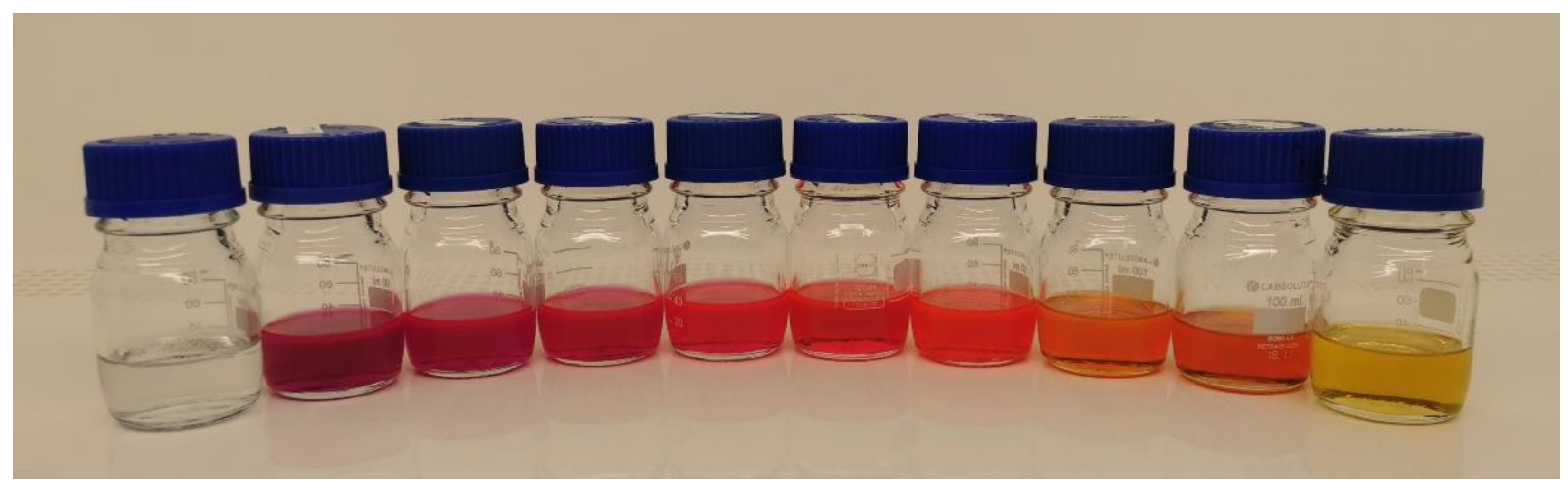
Figure 3.
Production steps for test paper manufacturing. (1) All components were mixed and stirred at 60 °C for 30 min. (2) Ultrasonic treatment was applied to ensure homogeneous distribution and to disperse the dye solids. (3) Pretreated cellulose strips were dip-coated in the emulsion for 20 s and dried overnight under ambient conditions by suspension in a fume hood.
Figure 3.
Production steps for test paper manufacturing. (1) All components were mixed and stirred at 60 °C for 30 min. (2) Ultrasonic treatment was applied to ensure homogeneous distribution and to disperse the dye solids. (3) Pretreated cellulose strips were dip-coated in the emulsion for 20 s and dried overnight under ambient conditions by suspension in a fume hood.
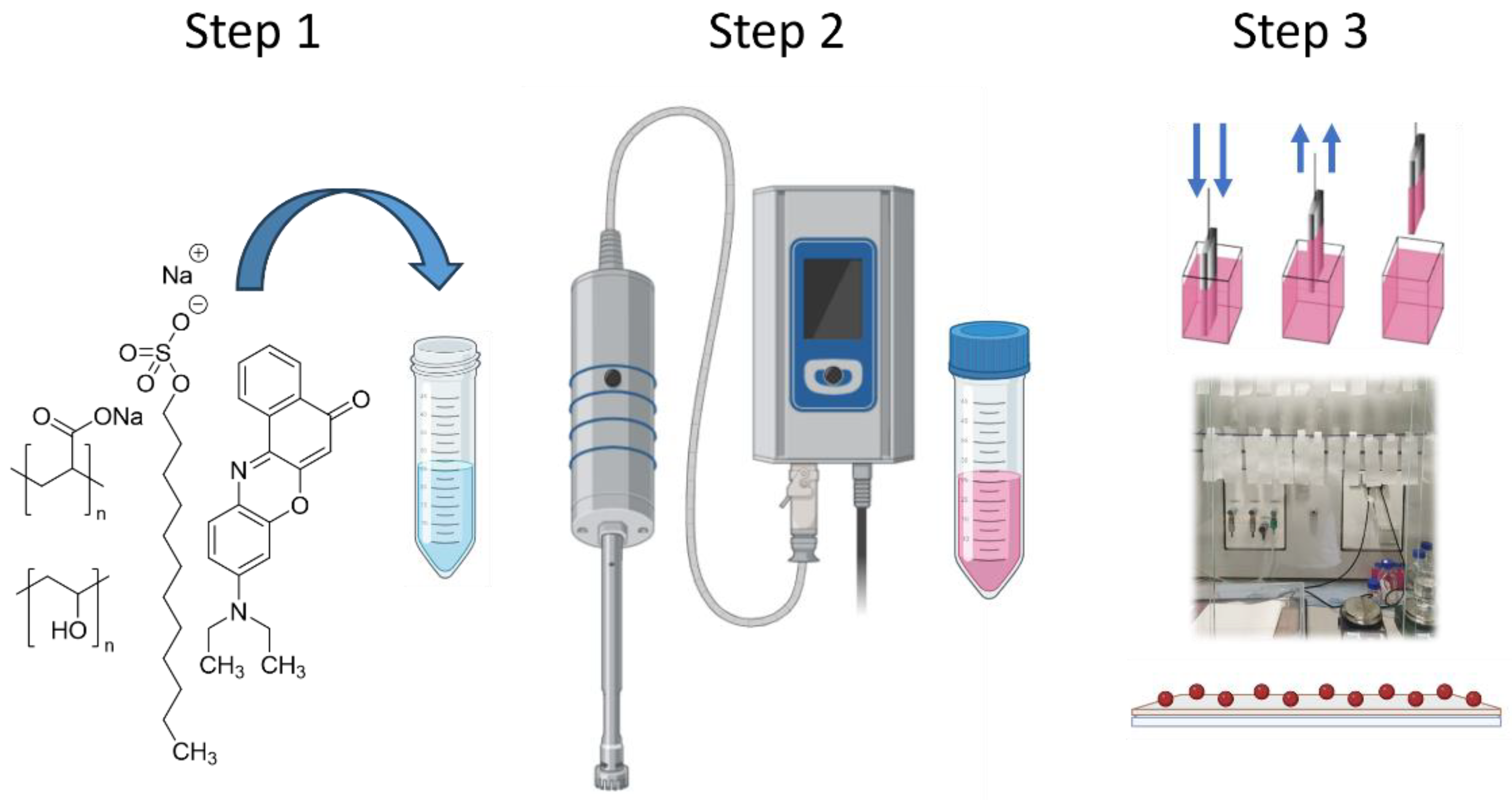
Figure 4.
Data-processing pipeline comprising four stages: (1) Image acquisition and calibration, (2) Hue-based segmentation and morphological refinement, (3) Object classification and centroid extraction, and (4) Georeferenced contamination-map generation.
Figure 4.
Data-processing pipeline comprising four stages: (1) Image acquisition and calibration, (2) Hue-based segmentation and morphological refinement, (3) Object classification and centroid extraction, and (4) Georeferenced contamination-map generation.
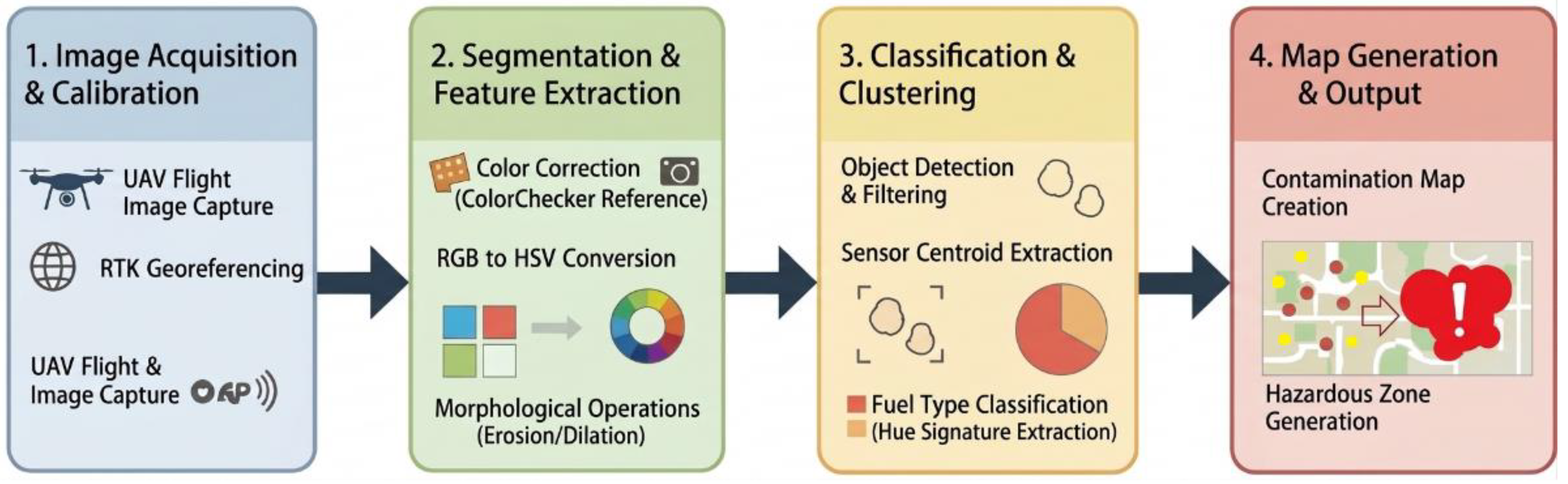
Figure 5.
Hue distribution of Nile red test papers after exposure to different liquid fuels. Hue values are expressed in degrees, with the angular position indicating the mean hue of each fuel type. The thickness of each sector represents the spread (variability) of the recorded values across replicates. Figures and a table with more solvents is shown in the supplement (Figure S8, Table S1).
Figure 5.
Hue distribution of Nile red test papers after exposure to different liquid fuels. Hue values are expressed in degrees, with the angular position indicating the mean hue of each fuel type. The thickness of each sector represents the spread (variability) of the recorded values across replicates. Figures and a table with more solvents is shown in the supplement (Figure S8, Table S1).
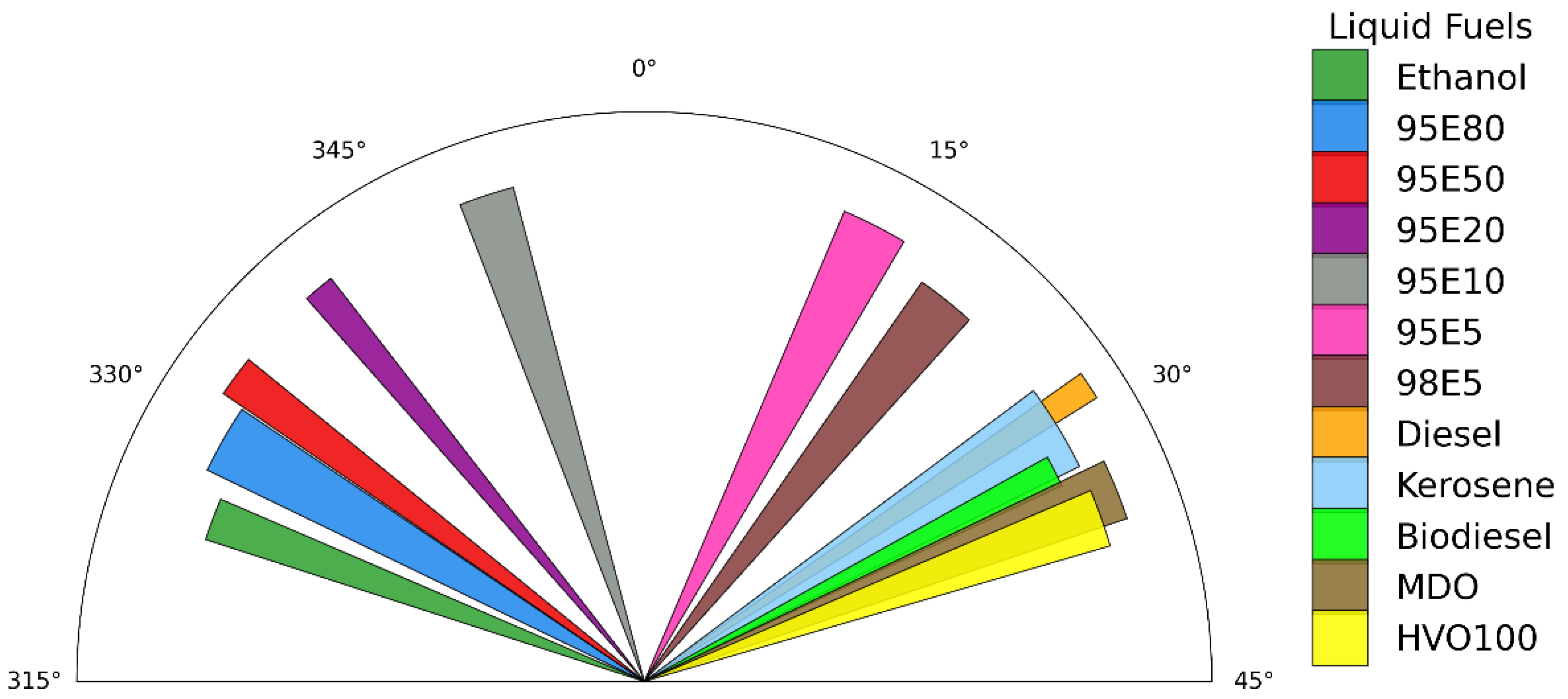
Figure 6.
Classification of gasoline (E5) and diesel by colorimetric hue value measured from Nile red test strips under laboratory conditions. (a) Frequency distribution of hue values showing complete separation between E5 (n = 20) and diesel (n = 20). (b) Individual hue values per measurement run with midpoint classification threshold (dashed line) and separation gap (green band). (c) Strip plot of all individual measurements with mean (black dot) and 95% confidence intervals. (d) Mean hue values with 95% confidence intervals; E5: 12.1 ± 2.5°, diesel: 28.2 ± 2.4° (Welch’s t-test, p < 0.001, Cohen’s d > 5, AUC = 1.0).
Figure 6.
Classification of gasoline (E5) and diesel by colorimetric hue value measured from Nile red test strips under laboratory conditions. (a) Frequency distribution of hue values showing complete separation between E5 (n = 20) and diesel (n = 20). (b) Individual hue values per measurement run with midpoint classification threshold (dashed line) and separation gap (green band). (c) Strip plot of all individual measurements with mean (black dot) and 95% confidence intervals. (d) Mean hue values with 95% confidence intervals; E5: 12.1 ± 2.5°, diesel: 28.2 ± 2.4° (Welch’s t-test, p < 0.001, Cohen’s d > 5, AUC = 1.0).
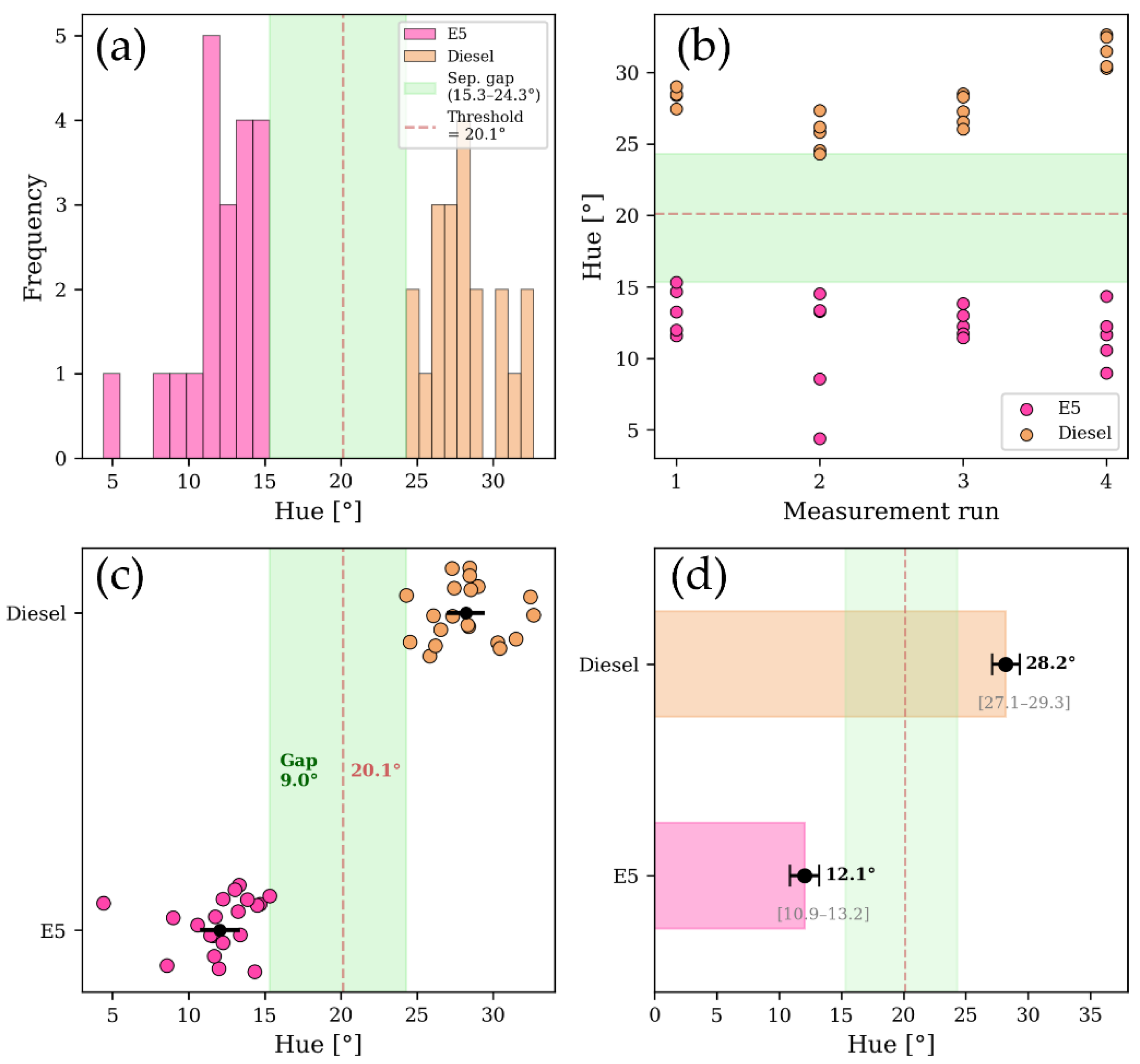
Figure 7.
Detection of gasoline-exposed test strips in UAV imagery using the image-processing workflow described in Section 2.4. (a) Original image “Frame 1”. (b) Positive detection events after HSV thresholding, filtering, and morphological operations. (c) Computed safety radii around detected clusters. (d) Final output image illustrating contamination zones for potential use by first responders. Result of diesel-exposed test strips are shown in the supplement Figure S11.
Figure 7.
Detection of gasoline-exposed test strips in UAV imagery using the image-processing workflow described in Section 2.4. (a) Original image “Frame 1”. (b) Positive detection events after HSV thresholding, filtering, and morphological operations. (c) Computed safety radii around detected clusters. (d) Final output image illustrating contamination zones for potential use by first responders. Result of diesel-exposed test strips are shown in the supplement Figure S11.
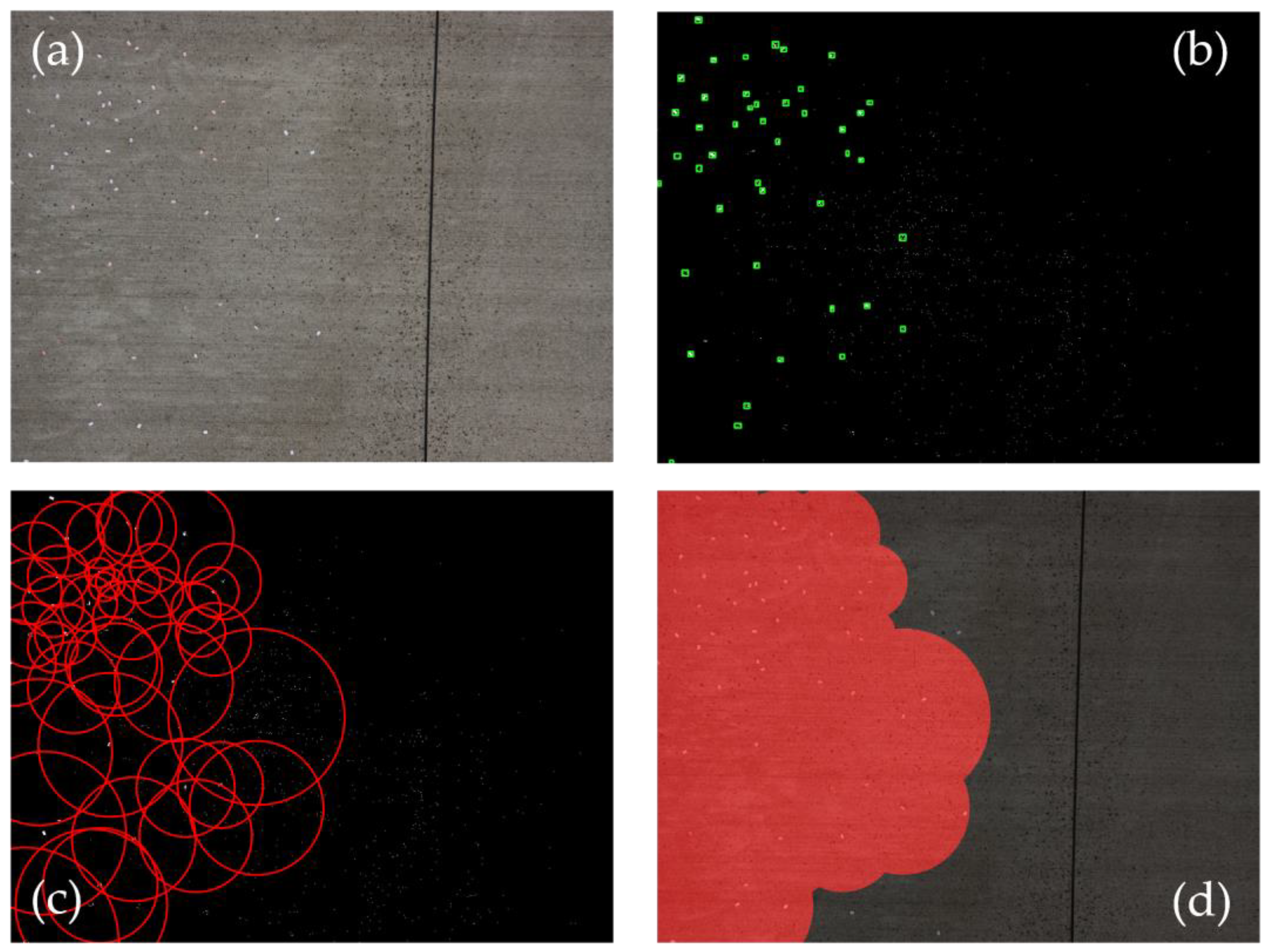

Table 1.
Spatial resolution of sensor strips (1 × 2 cm) as a function of UAV flight altitude. Pixel dimensions were determined from DJI Zenmuse H20T imagery at 10× optical zoom.
Table 1.
Spatial resolution of sensor strips (1 × 2 cm) as a function of UAV flight altitude. Pixel dimensions were determined from DJI Zenmuse H20T imagery at 10× optical zoom.
| Height (m) | 1 cm (px) horizontal |
1 cm (px) vertical |
2 cm (px) horizontal | 2 cm (px) vertical | Area (px) ± | ||
|---|---|---|---|---|---|---|---|
| 20 | 16.9 | 19.0 | 33.8 | 38.1 | 644 ± 42 | ||
| 30 | 11.3 | 12.7 | 22.6 | 25.4 | 286 ± 15 | ||
| 40 | 8.5 | 9.5 | 16.9 | 19.0 | 161 ± 8 | ||
| 50 | 6.8 | 7.6 | 13.6 | 15.2 | 103 ± 5 | ||
Table 2.
Laboratory characterization of twelve fuel types using Nile Red-impregnated cellulose test papers. Hue values, (n = 5 for all replicates) are reported as mean ± standard deviation (SD) with 95% confidence intervals (CI). Ethanol-containing gasoline blends show pronounced bathochromic shifts (hue 13 to 351°), while diesel-range fuels cluster at 28 to 35°. Low standard deviations (0.6 to 2.3°) indicate excellent measurement reproducibility.
Table 2.
Laboratory characterization of twelve fuel types using Nile Red-impregnated cellulose test papers. Hue values, (n = 5 for all replicates) are reported as mean ± standard deviation (SD) with 95% confidence intervals (CI). Ethanol-containing gasoline blends show pronounced bathochromic shifts (hue 13 to 351°), while diesel-range fuels cluster at 28 to 35°. Low standard deviations (0.6 to 2.3°) indicate excellent measurement reproducibility.
| Fuel Type | Mean Hue (°) | SD (°) | 95% CI |
|---|---|---|---|
| 98E5 | 19.2 | 1.5 | 17.4 – 21.1 |
| 95E5 | 13.4 | 1.6 | 11.3 – 15.4 |
| 95E10 | 351 | 1.3 | 349 – 352 |
| 95E20 | 340 | 0.7 | 339 – 341 |
| 95E50 | 333 | 0.9 | 332 – 334 |
| 95E80 | 330 | 1.6 | 328 – 332 |
| Ethanol | 325 | 1.1 | 323 – 326 |
| Diesel | 28.4 | 0.6 | 27.7 – 29.1 |
| Kerosene | 30.3 | 2.3 | 27.4 – 33.2 |
| Biodiesel | 31.5 | 0.7 | 30.6 – 32.4 |
| MDO | 33.6 | 1.4 | 31.9 – 35.4 |
| HVO100 | 34.9 | 1.4 | 33.2 – 36.7 |
Table 3.
UAV-based detection for Gasoline (95E5), frame-wise ground-truth validation.
| Metric | Frame 1 | Frame 2 | Frame 3 | Total |
|---|---|---|---|---|
| Positive Strips Deployed | 46 | 51 | 60 | 157 |
| TP | 44 | 43 | 52 | 139 |
| FN | 2 | 8 | 8 | 18 |
| Negative Strips Deployed | 7 | 10 | 12 | 29 |
| TN | 7 | 10 | 12 | 29 |
| FP | 0 | 0 | 0 | 0 |
| Sensitivity | 0.957 | 0.843 | 0.867 | 0.885 |
| Specificity | 1.000 | 1.000 | 1.000 | 1.000 |
| Precision | 1.000 | 1.000 | 1.000 | 1.000 |
| Accuracy | 0.962 | 0.869 | 0.889 | 0.903 |
| F1-Score | 0.978 | 0.915 | 0.929 | 0.939 |
Table 4.
UAV-based detection for Diesel (EN 590), frame-wise ground-truth validation.
| Metric | Frame 1 | Frame 2 | Frame 3 | Total |
|---|---|---|---|---|
| Positive Strips Deployed | 31 | 31 | 30 | 92 |
| TP | 30 | 29 | 30 | 89 |
| FN | 1 | 2 | 0 | 3 |
| Negative Strips Deployed | 23 | 16 | 23 | 62 |
| TN | 23 | 16 | 23 | 62 |
| FP | 0 | 0 | 0 | 0 |
| Sensitivity | 0.968 | 0.935 | 1.000 | 0.967 |
| Specificity | 1.000 | 1.000 | 1.000 | 1.000 |
| Precision | 1.000 | 1.000 | 1.000 | 1.000 |
| Accuracy | 0.982 | 0.957 | 1.000 | 0.981 |
| F1-Score | 0.984 | 0.966 | 1.000 | 0.983 |
Disclaimer/Publisher’s Note: The statements, opinions and data contained in all publications are solely those of the individual author(s) and contributor(s) and not of MDPI and/or the editor(s). MDPI and/or the editor(s) disclaim responsibility for any injury to people or property resulting from any ideas, methods, instructions or products referred to in the content. |
© 2026 by the authors. Licensee MDPI, Basel, Switzerland. This article is an open access article distributed under the terms and conditions of the Creative Commons Attribution (CC BY) license (http://creativecommons.org/licenses/by/4.0/).
Copyright: This open access article is published under a Creative Commons CC BY 4.0 license, which permit the free download, distribution, and reuse, provided that the author and preprint are cited in any reuse.