

Submitted:
06 May 2026
Posted:
07 May 2026
You are already at the latest version
Abstract
Forest structural diversity is a critical determinant of ecosystem function, yet the long-term influence of disturbance history on stand architecture remains complex. Here, we evaluate how historical disturbances shape structural and compositional diversity across 59 fully mapped plots in temperate mountain forests. Using field-based measurements, we quantified a suite of spatial, size-based, and compositional metrics, including Shannon entropy, diameter/height differentiation, species intermingling, and composite indices (SDI, Arten–Profill). Plots were categorized by time since disturbance (Recent, Intermediate, and Historical). Our results reveal a decoupling of structural recovery trajectories: biomass and tree size metrics (QMD, height, volume) follow a predictable, linear path of accumulation with disturbance age. In contrast, complex spatial indicators—such as SDI, species intermingling, and Clark–Evans aggregation—exhibit a threshold-based recovery pattern, increasing rapidly during early succession before plateauing as stands mature. Multivariate analyses (PCA and hierarchical clustering) indicate that forest maturity is not a monolithic structural endpoint; rather, late-successional stands diverge into multiple successional trajectories, each defined by unique spatial and size configurations. Compositional metrics showed lower sensitivity to disturbance history than structural indices, suggesting that structural heterogeneity is a more persistent "memory" of stand development than species composition alone. These findings suggest that structural complexity is a "built-in" feature of early stand development. Consequently, management strategies should shift from volume-centric goals toward trajectory-based approaches, employing early-successional interventions (e.g., variable-density thinning) to steer uniform stands toward complex, resilient structural configurations before developmental thresholds stabilize.
Keywords:
forest structure
; disturbance history
; structural diversity
; LiDAR
; species intermingling
; differentiation indices
; Carpathians
; montane forests
; PCA
; legacy effect
1. Introduction
Forests are among the most complex terrestrial ecosystems, supporting irreplaceable ecological, economic, and cultural functions across landscapes [1]. Their vertical and horizontal structure regulates energy exchange, water balance, carbon cycling, and biodiversity persistence [2]. These structural attributes emerge from interactions among site conditions, competition, disturbance, and management, and therefore provide a key lens for understanding how forests develop through time [3]. As global environmental change accelerates, assessing how historical legacies shape contemporary forest structure has become critical for conservation planning, sustainable management, and restoration [4]. Yet despite strong theoretical recognition of disturbance as a driver of forest heterogeneity, empirical evidence linking measurable historical events to present-day structural diversity remains surprisingly limited [5,6].
Forest structural diversity represents more than the distribution of tree size and height; it reflects spatial configuration, species intermingling, differentiation, and competitive relationships among individuals [7]. High structural diversity is often associated with increased habitat complexity, ecological resilience, and multi-layered canopies that support specialized flora and fauna [8]. Classic models of stand development predict that disturbance, natural or anthropogenic, can reset structural complexity, modify successional trajectories, and influence stand-scale biodiversity for decades to centuries[9]. However, the magnitude of these effects varies with disturbance intensity, timing, and spatial configuration [10]. Small-scale disturbance may enhance diversity by creating microsites and regeneration niches, whereas large-scale events may homogenize stands and limit recruitment opportunities [11]. These diverging pathways underscore the need for empirical assessments grounded in detailed structural metrics rather than broad categorical stand classifications.
Historical disturbances across Europe have dramatically influenced forest development [12]. Intensive harvesting, conversion to agriculture, and repeated management interventions simplified forest structure in many regions, reducing old-growth attributes and favoring even-aged cohorts [13]. More recently, partial abandonment of extractive uses, protection measures, and evolving silvicultural philosophies have permitted portions of Europe’s mountain forests to regain structural complexity [14].
Alongside climate-driven perturbations such as windthrow, drought, and bark beetle activity, these processes have created a mosaic of structural conditions spanning early successional stands to multi-layered forests with abundant large trees [15]. Yet despite the importance of these legacy effects, many forest inventories still emphasize composition and biomass while under-representing fine-scale spatial and structural features [16]. As a result, the relationships between disturbance history and structural outcomes remain insufficiently explored, especially at local scales relevant for forest management [17].
In recent years, novel terrestrial and aerial LiDAR technologies have transformed the quantification of forest structure [18]. These three-dimensional datasets allow measurement of tree attributes—diameter, height, crown geometry—and their spatial arrangement at unprecedented resolution[19,20,21] . Combined with plot-level field measurements, they permit estimation of core structural indicators including species richness, Shannon and Simpson diversity, diameter and height differentiation, Clark–Evans index for spatial pattern, competition indices, and intermingling of competing species [22]. This multidimensional analytical capability enables clearer understanding of how structural diversity varies among stands with contrasting disturbance histories. However, although LiDAR-based structural analyses have rapidly proliferated [23,24], applications linking them to legacies of historical disturbance remain sparse [25]. Most studies address stand attributes as a function of current conditions, ignoring past dynamics that may have constrained or catalysed structural complexity.
Disturbance history can influence contemporary forest structure through several mechanisms [26]. Direct removal of biomass (e.g., selective logging, clearcutting) alters size distributions and reduces vertical layering[27]. Subsequent regeneration pathways depend on disturbance timing, species traits, and local competition. In some cases, historical harvesting encourages species coexistence by reducing dominance hierarchies, while in others it homogenizes stands and suppresses long-term complexity [28]. Similarly, large natural disturbances – windthrow, fire, or beetle outbreaks—generate heterogeneous microsites that support structural differentiation. These legacies persist as variation in tree size distributions, competitive interactions, spatial aggregation, and species intermingling [29]. Empirical studies in European montane forests have demonstrated that past disturbance can increase overall heterogeneity, but effects vary considerably across landscapes. The need to evaluate how these dynamics operate within specific forest mosaics remains critical, as sustainable management increasingly seeks to emulate natural structural variability [30].
Forest structure is also strongly associated with biodiversity outcomes. Vertical and horizontal complexity create ecological niches that support specialist species, regulate microclimates, and buffer environmental extremes [31]. The spatial intermixing of species influences competition and niche partitioning, thereby contributing to functional diversity [32]. Differentiation among individuals in height and diameter is a key marker of succession and developmental stage, with greater variation typically associated with mixed-age cohorts and reduced management intensity [33]. These features provide clues about the stand’s developmental trajectory and capacity to maintain ecosystem services under changing environmental conditions. Yet, despite the ecological importance of such structural attributes, their relationships with past disturbance patterns are often inferred rather than directly measured.
Because disturbance regimes vary temporally and spatially, their influence on structural diversity may not emerge consistently across all indicators. For example, richness-based compositional metrics (Margalef, Shannon, or Simpson indices) may reflect recent regeneration patterns but not capture spatial processes [34]. Spatial or differentiation indices such as Clark–Evans, diameter differentiation, height differentiation, intermingling provide complementary insights about stand organization that relate more directly to legacy conditions. Integrating this suite of indicators provides a more holistic understanding of structural diversity and allows detection of subtle legacies that simpler metrics miss. Given increasing availability of LiDAR-derived forest inventories, such analytical frameworks are becoming more accessible and reliable [35] .
Despite conceptual consensus that disturbance legacies matter, most empirical studies focus either on large-scale regional trends or on individual stands [36]. Few combine detailed structural measurements with explicit spatially mapped disturbance history [34]. As a result, evidence remains fragmented regarding how strongly, and through which pathways, disturbances shape local structural diversity. Understanding these dynamics is key for silvicultural strategies that seek to promote ecological resilience and emulate natural patterns. Management plans increasingly prioritize diversification of stand structure, but interventions require robust reference conditions informed by empirical data [37].
To address these gaps, our overarching goal is to determine whether historical disturbances exert a persistent influence on present-day forest structural diversity. Specifically, we aim: i) to quantify the sensitivity of specific structural dimensions to disturbance history, by evaluating how compositional, spatial, and size-differentiation indices respond to disturbance categories and time since disturbance, identifying which metrics best capture legacy effects; and ii) to assess multivariate structural trajectories, determining through ordination and clustering whether forest stands with different disturbance histories converge toward a uniform mature state or diverge into distinct structural configurations.
2. Materials and Methods
2.1. Study Area
The study was conducted in a mountainous forest landscape in the Romanian Carpathians (Figure 1). The region is characterized by steep terrain, elevations ranging from approximately 900–1,600 m, and a temperate-continental climate with strong orographic influence. Annual precipitation exceeds 1,200 mm, with rain and wet snow dominating cold-season inputs. Forests are dominated Norway spruce (Picea abies), followed byEuropean beech (Fagus sylvatica) and silver fir (Abies alba), forming structurally varied mixed montane stands typical of the Carpathian range [38].
Forest management interventions have historically included selective logging, salvage logging, and local clearcutting. More recent protection and reduced harvesting intensity have allowed partial regeneration and development of structurally complex patches. The study area presents a mosaic of plots that experienced historical disturbances and others that appear structurally intact, offering an opportunity to compare development patterns [38].
2.2. Data
2.2.1. Disturbance History
Disturbance histories were reconstructed from existing geospatial layers describing historical and recent disturbances, including selective harvests, salvage logging, and moderate to severe canopy loss [26,38]. Reference layers were derived from satellite image chronologies, historical spy satelites, and forest management records. For the oldest disturbances D3C1206-200249F065 Corona Spy Satellite was used (Figure 2). The disturbance database was completed with a compilation of data from various sources and studies [5,26,39,40,41,42]
Disturbances were binarily assigned to each plot based on overlap with disturbance polygons classified as either: historical disturbance (> 70 years), intermediate disturbance (40–70 years), recent disturbance (< 40 years). Plots were consequently grouped into disturbance categories for subsequent analysis.
2.2.2. Field and LiDAR-Derived Tree Measurements
A total of 59 fixed-area sampling plots were used for structural assessment. Each plot was fully mapped and surveyed using a combination of Mobile Laser Scanning (MLS) and field measurements. The plots were scanned using ZEB Horizon, a scanner based on LiDAR technology. The scanner uses a rotating mirror to beam around the area that is scanned. The measurement characteristics consist of up to 300,000 repetitions per second. Data acquired using GEOSLAM Horizon technology is a point cloud in the form of three-dimensional data compiled using SLAM (simultaneous localization and mapping). Tree attributes including species identity, diameter at breast height (DBH), total height, and spatial coordinates were obtained either directly in the field or through LiDAR-assisted extraction. Individual tree volume was estimated from species-specific allometric equations .
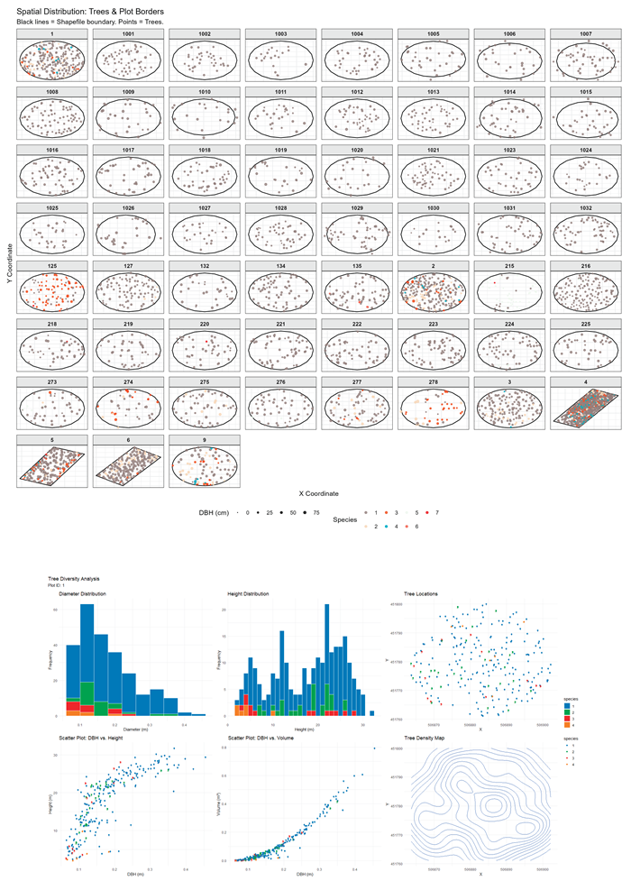
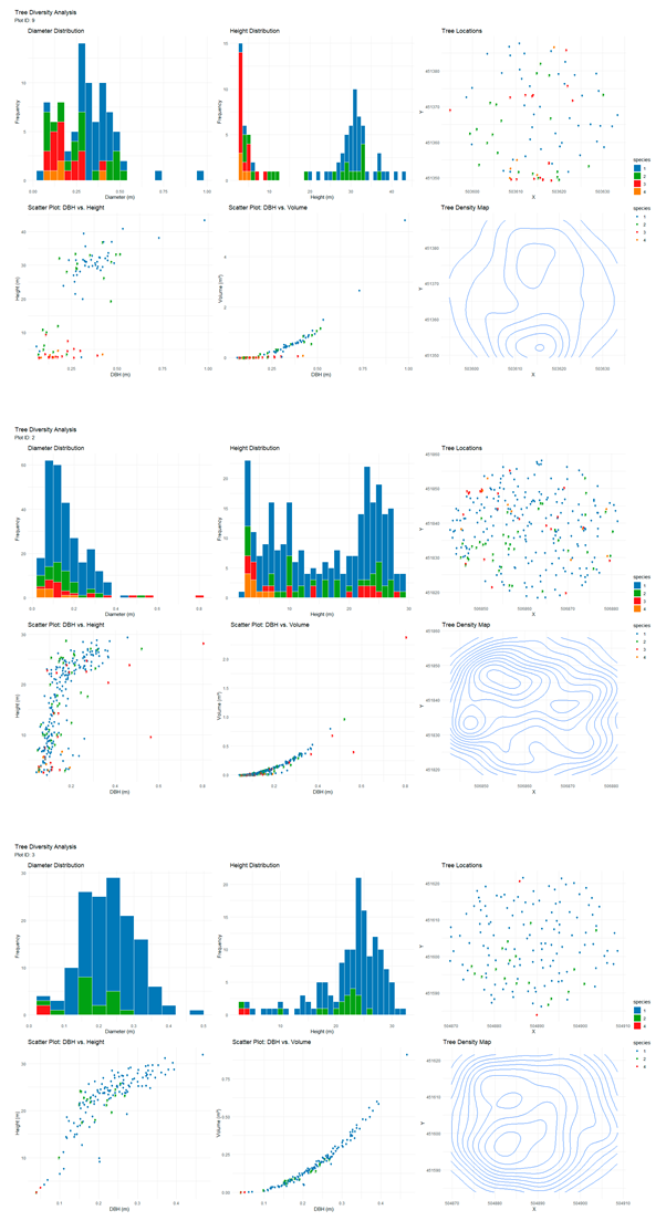
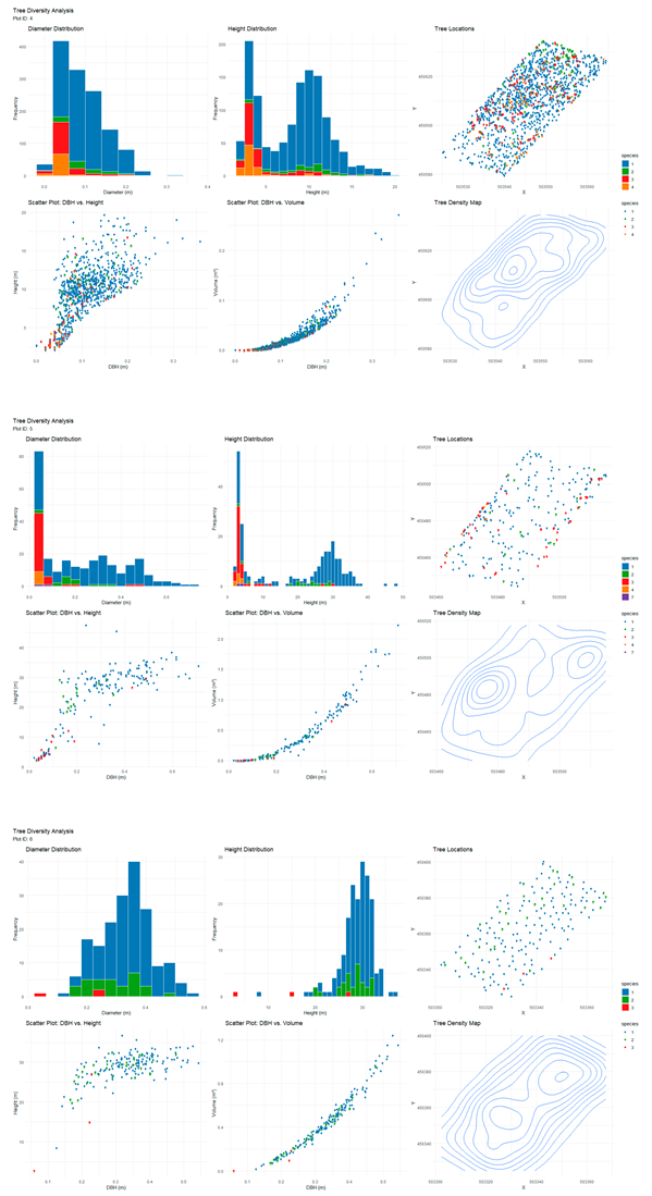
The resulting tree inventory dataset contained DBH and height distributions, species composition, and precise three-dimensional stem locations for each plot (Figure 2). These metrics provided the necessary basis for computing structural diversity indices (Appendix A1).
2.3. Structural Diversity Indices
Regarding Compositional Indices we calculated a set of widely used indices to quantify diversity of species composition within plots: Margalef species richness index, Shannon–Wiener entropy, Simpson’s index (λ), and Pielou’s evenness. These indices summarize species presence and proportional abundance, providing insight into composition independent of spatial structure.
For Size Differentiation the DBH and height heterogeneity were evaluated using the diameter differentiation index and the height differentiation index. Both measure how tree dimensions vary among neighbours, reflecting competition gradients or cohort structure.
On Spatial Pattern and Intermingling the Horizontal structure was evaluated via the Clark–Evans index, quantifying aggregation vs. regularity, and the species intermingling index, describing spatial mixing of species pairs.
Regarding competition and overall diversity to reflect competitive interactions and integrate multiple structural dimensions, we computed the Bella competition index, the Jaehne & Dohrenbusch total diversity index, and the Arten–Profill index. These composite metrics summarize neighbourhood interactions, structural complexity, and functional heterogeneity.
All indices were computed at the plot scale using tree positions and measured attributes. As common in forest inventories only trees above the minimum DBH threshold of 8 cm were included. Mathematical definitions for all calculated indices are provided in Appendix A2.
2.4. Statistical Analysis
All statistical analyses were performed in the R statistical computing environment, utilizing the ‘vegan’ package for diversity metrics, ‘spatstat’ for spatial point pattern analysis, and ‘mgcv’ for generalized additive modeling.
To address the first objective of quantifying the sensitivity of structural dimensions to disturbance history we adopted a dual approach evaluating both categorical differences and continuous temporal trends. First, structural indices were aggregated by plot and compared across the four disturbance categories (Recent, Intermediate, Historical, and Undisturbed). Due to the non-normal distribution of the data, differences between groups were tested using the non-parametric Kruskal–Wallis test. Significant results were followed by pairwise Wilcoxon rank-sum tests with a Bonferroni correction to adjust for multiple comparisons. Second, to evaluate temporal recovery trajectories, disturbance age was treated as a continuous predictor. We assessed monotonic relationships between age and structural indices using Spearman’s rank correlation coefficients. Additionally, to detect potential non-linear recovery patterns (e.g., rapid early structural development followed by saturation), we fitted Generalized Additive Models (GAMs) using thin plate regression splines and compared these trends against linear models.
To address the second objective of assessing multivariate structural trajectories we performed a multivariate analysis to determine whether stands converge or diverge over time. All structural indices were first standardized (Z-score scaling) to account for differences in measurement units. We conducted a Principal Component Analysis (PCA) to reduce dimensionality and identify the primary gradients of structural variation. Subsequently, to classify stands based on their multidimensional structural signatures, we performed hierarchical clustering on the Euclidean distance matrix using Ward’s minimum variance method (ward.D2). The resulting clusters were analyzed via contingency tables to assess their correspondence with the original disturbance categories.
3. Results
3.1. General Structural Characteristics and Raw Data Distribution
The 59 analysed forest plots covered a comprehensive range of development stages, from young regeneration phases to mature, fully stocked stands. Plot ages spanned a broad chronosequence from 10 to 130 years, ensuring that the dataset captures the full trajectory of post-disturbance recovery (Table A1).
Figure 3.
Raw metric data plots.
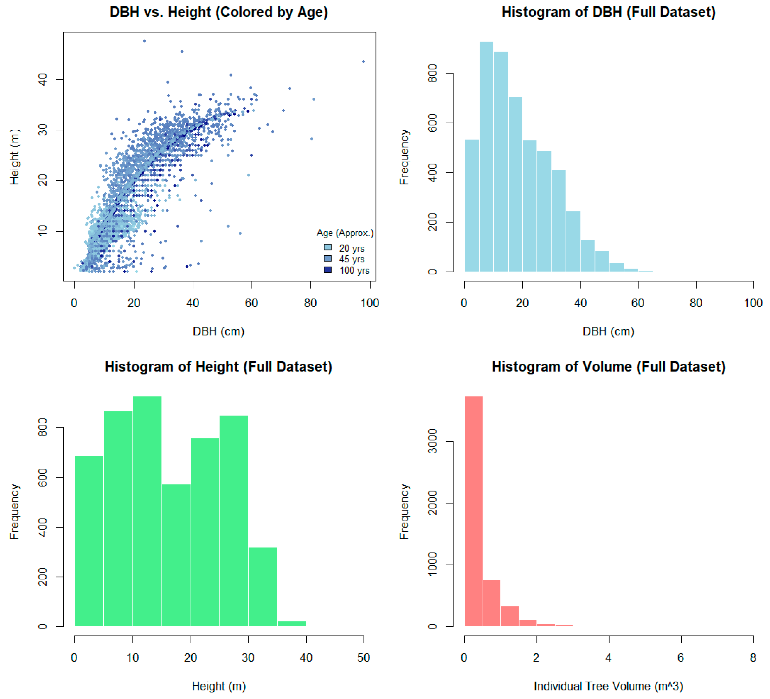
Structural attributes varied widely across this gradient. Quadratic Mean Diameter (QMD) ranged from 10.7 cm in dense young stands to 36.2 cm in mature forests, while mean heights varied from 9.1 m to 29.0 m. This structural heterogeneity was further reflected in wood volume and basal area, which showed distinct patterns based on stand origin. Planted stands generally exhibited higher stocking levels, with basal areas reaching up to 102.8 m²/ha and volumes peaking at approximately 1148 m³/ha, reflecting the uniform spacing and rapid initial biomass accumulation typical of silvicultural establishment. In contrast, naturally regenerated stands, while also capable of reaching high volumes (up to 1136 m³/ha at maturity), displayed greater variability in stem density (ranging from 745 to 2971 trees/ha) compared to the extreme density ranges sometimes observed in younger planted plots (610–11,405 trees/ha). Older natural stands (>100 years) typically maintained lower stem densities but larger individual tree dimensions, consistent with self-thinning processes and gap dynamics. The complete inventory of plot-level structural metrics is provided in Appendix B.
3.2. Sensitivity of Structural Dimensions to Disturbance History
When analysing specific structural dimensions, distinct patterns emerged regarding disturbance history (Table A2). Compositional metrics revealed a stark contrast within the landscape; while some mixed stands reached Shannon entropy values of 0.5–0.6, a significant proportion of the dataset—particularly planted stands in the 30–45 year range—exhibited values approaching 0.00 for Margalef richness, Shannon entropy, and Simpson’s index. This quantifies the presence of widespread monocultures where compositional diversity is effectively null, regardless of stand age.
Horizontal and size-based structures exhibited significantly stronger gradients than composition alone. The Clark–Evans aggregation index showed high variability, ranging from values indicating strong clustering in young, recently disturbed regeneration to values exceeding 1.0 in older or thinned stands, which shifted toward random or regular distributions. Similarly, the species intermingling index tracked the monoculture-to-mixed gradient; numerous plots showed minimal intermingling, whereas structurally complex natural plots approached values of 1.0, indicating that nearest neighbors in these stands are almost always different species. Diameter differentiation remained consistently high across the dataset, generally ranging between 0.80 and 0.95, indicating that even in monocultures, substantial neighborhood-scale variation in tree size exists (Figure 4). Height differentiation showed a similar tendency, with the wide range of differentiation within old plots suggesting the development of multiple cohorts.
Competition intensity (Bella index) showed extreme variability, peaking in dense young stands and generally decreasing in mature, thinned stands. Composite indices demonstrated separation among disturbance histories; Total Diversity (SDI) and the Arten–Profill (APi) index provided a multidimensional view that compositional indices often missed. While these indices showed clear categorical differences, they did not exhibit strictly linear increases across the chronosequence (Table 1), suggesting that structural complexity accrues rapidly in early succession but levels off as stands reach a threshold of maturity (Figure 5).
Wood volume per hectare and basal area differed notably according to stand origin. Planted plots showed higher basal area on average, peaking at 102.8 m²/ha, alongside higher total stand volume, reflecting the uniformity and density of silvicultural establishment. In contrast, naturally regenerated plots exhibited broader variation in these metrics, consistent with more variable disturbance histories (Figure 6).
The analysis of continuous disturbance age (Table 1) clarified these trends. While categorical tests (Kruskal-Wallis) suggested rapid early recovery, linear correlations with disturbance age were strongest for size and stocking metrics. Quadratic mean diameter (QMD) showed a significant positive correlation (rho = 0.62, p < 0.001), as did mean height (rho = 0.50, p < 0.001). Furthermore, basal area (rho = 0.32, p < 0.05) and total volume (rho = 0.41, p < 0.01) showed significant positive linear relationships with age. Conversely, stem density decreased significantly (rho = -0.38, p < 0.01) as stands self-thinned.
Despite the clear categorical separation between recent and old stands, complex structural indices (Shannon entropy, Intermingling, SDI, APi, and Clark-Evans) did not exhibit significant linear correlations with disturbance age (Table 1). This indicates that structural complexity increases significantly in the initial decades following disturbance (creating the contrast seen in categorical tests) but does not follow a strict monotonic trajectory in later succession, effectively plateauing once maturity is reached (Figure 6). The DBH–height relationship (Figure 3) further supports this, showing that older stands are defined more by the presence of tall, large-diameter trees rather than by continually increasing spatial complexity.
3.3. Multivariate Structural Trajectories
To synthesize the multi-dimensional nature of stand structural responses to disturbance, we utilized a multivariate approach combining Principal Component Analysis (PCA) and Hierarchical Cluster Analysis (HCA). The PCA revealed that 66.4% of the total variance was explained by the first two axes, indicating strong structural gradients within the dataset (Figure 7).
PC1 (45.5% of variance) represented a “Structural Complexity” gradient. Metrics associated with stand heterogeneity, such as species intermingling, Clark–Evans, SDI, and Shannon entropy, loaded heavily along this axis. This confirms that spatial arrangement and compositional diversity covary strongly, acting as a primary axis of differentiation among plots. PC2 (20.9% of variance) captured a “Developmental/Size” gradient, characterized by positive loadings for QMD, Volume per hectare, and Basal Area, which opposed stem density. This axis effectively separates stands based on their biomass accumulation and thinning stage, independently of their compositional complexity.
Hierarchical clustering (Ward’s method, k=4) provided a robust validation of these gradients, identifying distinct structural typologies (Figure 8). The dendrogram revealed that disturbance history acts as the primary organizing factor, yet it highlighted that older stands do not converge toward a single “old-growth” condition. Instead, they diverged into multiple unique structural configurations. One cluster was dominated by stands with lower structural complexity, characteristic of recent disturbances or dense, uniform regeneration. In contrast, the remaining clusters grouped older and undisturbed plots, but these split into distinct sub-branches based on their specific developmental trajectory (e.g., volume-driven maturity versus diversity-driven complexity).
The Silhouette analysis (mean width = 0.34) supports the distinctness of these groupings, confirming that while some intermediate overlap exists, the stands possess identifiable structural signatures linked to their disturbance legacies. Collectively, these multivariate results underscore that while disturbance sets the starting point for recovery, the subsequent developmental path—governed by site-specific factors and thinning—leads to a diversification of structural forms rather than simple, linear progression.
4. Discussion
Forest structural diversity is the emergent property of disturbance history, successional time, and competitive dynamics. While traditional forest models often view structural development as a linear progression toward maturity, the results presented here reveal a more complex, threshold-based trajectory. Our analysis demonstrates that while biomass and tree size metrics exhibit continuous growth, spatial and compositional indices reach a threshold of complexity relatively early in stand development, after which they stabilize. These findings underscore that disturbance history acts as a primary “filter” for early stand configuration, while subsequent development is characterized by divergence rather than convergence toward a single structural state.
4.1. Legacy Effects on Stand Structure
The structural diversity of temperate mountain forests is not merely a product of current environmental conditions, but a persistent reflection of historical disturbance legacies. Our results demonstrate that stand structure—particularly size hierarchy and spatial configuration—functions as a long-term “memory” of past canopy events. We observed a clear bifurcation in how stand attributes respond to time since disturbance: while size-based and biomass metrics (QMD, height, and volume) correlate significantly with age in a linear fashion, complex spatial and compositional indices exhibit a threshold-based recovery pattern.
The rapid recovery of structural complexity in the early decades following disturbance is consistent with the “stand initiation” and “stem exclusion” stages defined by stand dynamics [9,43]. Our finding that spatial indices (e.g., Clark–Evans, intermingling) plateau after a certain age suggests that once the canopy closes and vertical stratification begins, the spatial “rules” of the stand are established [43]. Thereafter, the stand continues to accumulate biomass, but its fundamental structural “type” remains anchored to the dynamics of its initial regeneration phase. This aligns with findings by Bauhus et al. 2009, who emphasize that silvicultural interventions early in stand development have a disproportionate influence on creating or inhibiting future old-growth structural attributes [37].
Conversely, the significant positive linear correlations between disturbance age and metrics such as QMD (rho = 0.62) and height (rho = 0.50) confirm that biomass accumulation follows a more predictable, long-term monotonic trajectory. This is the hallmark of density-dependent development, where competition drives the size distribution toward larger individuals, a process well-documented in temperate systems [44,45]. The fact that competition intensity (Bella index) did not emerge as a primary differentiator of disturbance legacy supports the theory that, in mixed-species stands, canopy architecture and niche partitioning often mitigate competitive stress more effectively than in uniform plantations [46].
Finally, the persistent difference between planted and natural stands reinforces the concept of “silvicultural legacy.” Planted stands displayed higher maximum stocking levels, likely due to the removal of initial competitive bottlenecks through uniform spacing. As suggested by recent research, the long-term structural resilience of these forests is better predicted by the heterogeneity established during the regeneration phase than by the simple age of the stand [47,48].
4.2. Multidimensional Patterns and Structural Trajectories
Our multivariate analysis reveals that forest structure is not a unidirectional outcome of time, but a multidimensional surface defined by two primary gradients: a “Structural Complexity” axis and a “Developmental/Size” axis. The PCA captured 66.4% of the total variance, confirming that plot configurations are governed by distinct spatial and size-based drivers.
The first axis (PC1, 45.5% variance) reflects a structural complexity gradient, heavily loaded by species intermingling, SDI, and the Clark–Evans aggregation index. This aligns with the “structural complexity hypothesis” proposed by McElhinny et al. (2005), which posits that spatial heterogeneity and niche diversity are emergent properties distinct from biomass accumulation [49]. Our results suggest that spatial arrangement is an independent dimension of stand development; stands can accumulate significant biomass (PC2) while remaining spatially simple, or conversely, achieve high spatial complexity with relatively low volume.
The hierarchical clustering results provide critical insight into the successional trajectory of these stands. The dendrogram reveals that while disturbance history acts as the primary organizing factor (separating recent disturbances from historical ones), older stands diverge into multiple successional trajectories rather than converging toward a single “old-growth” condition. This lack of convergence supports the stochastic gap dynamics model, which argues that late-successional forests are mosaics where site-specific microsite conditions and historical gap frequencies produce distinct structural neighborhoods [50,51]. Our findings emphasize that forest maturity is not a monolithic structural endpoint, but a process of structural diversification, where local competitive interactions and individual tree mortality continuously reorganize the stand [52].
4.3. Management and Conservation Implications
Our findings suggest that forest management strategies should shift from a focus on volume to the active promotion of structural complexity. Because spatial complexity plateaus early in development, late-stage interventions in uniform plantations are often insufficient to restore structural diversity. To steer stands toward complexity, silvicultural treatments such as variable density thinning (VDT) or gap-based harvesting should be applied during the early-to-mid successional stages (30–50 years) to foster heterogeneity before the stand architecture stabilizes [53,54].
Furthermore, the divergence observed in older stands indicates that maturity is not a monolithic endpoint. Consequently, management should abandon single-target structural goals. Instead, we advocate for trajectory-based management that promotes a landscape-level mosaic of developmental pathways. By recognizing and maintaining the diverse configurations that emerge naturally in complex stands, managers can foster resilience against climate-driven disturbances [27]. Finally, we recommend that forest management plans incorporate spatial and compositional indicators—specifically SDI, species intermingling, and diameter differentiation—as key performance indicators (KPIs) alongside production goals.
5. Conclusions
Historical disturbances act as long-term architects of mountain forest structure, leaving persistent legacies that endure long after compositional signatures have stabilized. This study reveals that forest development is not a uniform progression toward a single structural endpoint, but a multidimensional process marked by early-stage threshold dynamics and long-term successional divergence. We found a clear decoupling between structural dimensions: while biomass and tree size follow linear, predictable growth, spatial complexity indices—such as species intermingling, diameter differentiation, and spatial aggregation—reach developmental thresholds relatively early in a stand’s life. Crucially, older stands do not converge toward a monolithic “old-growth” structure; rather, they diverge into varied successional pathways, highlighting that heterogeneity is an inherent, vital property of forest maturity rather than a transient phase.
These findings necessitate a paradigm shift from volume-centric management toward trajectory-based approaches that prioritize structural resilience. Since spatial complexity stabilizes early, late-stage interventions in uniform plantations are often inadequate to restore natural heterogeneity. Effective management requires proactive measures—such as variable-density thinning or gap-based harvesting—applied during early-to-mid successional stages (30–50 years) to steer stands toward complex, resilient configurations. By adopting spatial and size-based indicators, such as SDI and species intermingling, as key performance indicators alongside traditional production goals, forest managers can foster the landscape-level mosaic of developmental pathways necessary to ensure long-term ecological function and climate adaptability.
Appendix A
Appendix A.1
| Plot id | Origin | Average age (years) | Plot area (m2) | Trees per hectare | Quadric Mean Diameter (cm) | Quadric Mean Height (m) | Basal area (m2/ha) | Volume (m3/ha) |
| 1 | Planted | 45 | 1250 | 1984 | 19.5 | 19.1 | 59.0 | 407.37 |
| 1001 | Planted | 35 | 300 | 2170 | 19.4 | 17.7 | 64.2 | 559.66 |
| 1002 | Planted | 45 | 300 | 1153 | 23.1 | 21.4 | 48.3 | 431.91 |
| 1003 | Planted | 45 | 300 | 678 | 24.2 | 21.8 | 31.2 | 289.10 |
| 1004 | Planted | 35 | 300 | 1322 | 22.5 | 20.5 | 52.7 | 463.65 |
| 1005 | Planted | 65 | 300 | 1085 | 29.7 | 25.5 | 75.1 | 742.02 |
| 1006 | Planted | 65 | 300 | 949 | 29.7 | 25.5 | 65.7 | 645.30 |
| 1007 | Natural | 90 | 300 | 1865 | 27.1 | 23.3 | 107.3 | 1062.02 |
| 1008 | Planted | 45 | 300 | 2678 | 19.4 | 18.7 | 79.1 | 658.99 |
| 1009 | Natural | 85 | 300 | 1051 | 36.2 | 27.9 | 108.3 | 1136.34 |
| 1010 | Natural | 65 | 300 | 746 | 33.7 | 27.3 | 66.4 | 675.93 |
| 1011 | Planted | 45 | 300 | 881 | 27.9 | 22.5 | 54.0 | 545.34 |
| 1012 | Planted | 45 | 300 | 1390 | 22.4 | 20.0 | 54.7 | 519.52 |
| 1013 | Planted | 35 | 300 | 1492 | 18.9 | 18.1 | 41.8 | 361.01 |
| 1014 | Planted | 40 | 300 | 1458 | 27.8 | 23.9 | 88.3 | 868.24 |
| 1015 | Natural | 85 | 300 | 1119 | 27.3 | 23.9 | 65.5 | 629.12 |
| 1016 | Natural | 105 | 300 | 2475 | 21.2 | 19.4 | 87.3 | 801.01 |
| 1017 | Natural | 105 | 300 | 1458 | 28.9 | 24.3 | 95.5 | 939.78 |
| 1018 | Planted | 35 | 300 | 1492 | 28.0 | 22.6 | 92.0 | 891.47 |
| 1019 | Natural | 130 | 300 | 848 | 31.0 | 23.0 | 64.0 | 652.32 |
| 1020 | Planted | 55 | 300 | 814 | 31.2 | 26.3 | 62.0 | 623.17 |
| 1021 | Planted | 35 | 300 | 1932 | 16.8 | 16.4 | 42.9 | 366.59 |
| 1023 | Natural | 105 | 300 | 1254 | 25.6 | 22.5 | 64.7 | 599.94 |
| 1024 | Planted | 45 | 300 | 915 | 19.3 | 18.4 | 26.8 | 235.25 |
| 1025 | Planted | 35 | 300 | 949 | 26.1 | 22.4 | 50.6 | 496.47 |
| 1026 | Natural | 90 | 300 | 1119 | 30.1 | 24.5 | 79.8 | 809.17 |
| 1027 | Planted | 35 | 300 | 881 | 21.2 | 20.0 | 31.2 | 281.54 |
| 1028 | Planted | 35 | 300 | 1695 | 19.8 | 18.5 | 52.1 | 465.50 |
| 1029 | Planted | 30 | 300 | 1831 | 23.8 | 20.8 | 81.7 | 783.68 |
| 1030 | Planted | 45 | 300 | 610 | 22.5 | 20.9 | 24.2 | 221.13 |
| 1031 | Planted | 40 | 300 | 1390 | 25.3 | 22.9 | 69.9 | 671.03 |
| 1032 | Planted | 30 | 300 | 2068 | 19.8 | 18.7 | 63.8 | 576.49 |
| 125 | Natural | 30 | 500 | 2035 | 15.1 | 11.4 | 36.5 | 295.05 |
| 127 | Planted | 50 | 500 | 1811 | 22.5 | 21.5 | 71.7 | 833.20 |
| 132 | Planted | 55 | 500 | 611 | 32.9 | 24.8 | 52.0 | 640.22 |
| 134 | Planted | 50 | 500 | 1547 | 25.7 | 24.5 | 80.0 | 1014.63 |
| 135 | Planted | 45 | 500 | 1384 | 26.3 | 21.3 | 75.2 | 839.35 |
| 2 | Planted | 45 | 1250 | 2167 | 19.2 | 18.0 | 62.6 | 418.03 |
| 215 | Natural | 10 | 500 | 1160 | 11.1 | 9.2 | 11.2 | 49.85 |
| 216 | Natural | 30 | 500 | 2971 | 16.2 | 12.6 | 61.2 | 426.75 |
| 218 | Natural | 90 | 500 | 936 | 27.4 | 23.3 | 55.3 | 722.26 |
| 219 | Natural | 90 | 500 | 895 | 29.6 | 21.3 | 61.8 | 668.75 |
| 220 | Natural | 115 | 500 | 855 | 26.7 | 17.8 | 47.9 | 428.48 |
| 221 | Natural | 100 | 500 | 1282 | 25.9 | 19.0 | 67.5 | 669.66 |
| 222 | Natural | 80 | 500 | 1201 | 27.5 | 21.0 | 71.4 | 745.58 |
| 223 | Natural | 80 | 500 | 1547 | 21.3 | 16.2 | 55.0 | 489.82 |
| 224 | Planted | 50 | 500 | 1241 | 24.9 | 22.9 | 60.5 | 702.79 |
| 225 | Planted | 50 | 500 | 834 | 30.3 | 22.3 | 60.3 | 641.22 |
| 273 | Planted | 55 | 500 | 957 | 28.7 | 24.9 | 61.8 | 798.54 |
| 274 | Planted | 55 | 500 | 957 | 26.6 | 19.9 | 53.2 | 648.26 |
| 275 | Planted | 55 | 500 | 1180 | 30.6 | 26.6 | 86.5 | 1145.35 |
| 276 | Planted | 55 | 500 | 997 | 29.8 | 26.9 | 69.7 | 911.50 |
| 277 | Planted | 50 | 500 | 1323 | 29.2 | 24.5 | 88.5 | 1148.07 |
| 278 | Planted | 45 | 500 | 875 | 30.1 | 18.2 | 62.4 | 688.31 |
| 3 | Natural | 40 | 1250 | 1139 | 23.8 | 23.3 | 50.8 | 388.93 |
| 4 | Planted | 20 | 1125 | 11406 | 10.7 | 9.1 | 102.8 | 710.50 |
| 5 | Planted | 60 | 2250 | 1109 | 28.5 | 22.0 | 70.9 | 626.80 |
| 6 | Planted | 60 | 2680 | 680 | 34.2 | 29.0 | 62.4 | 532.20 |
| 9 | Planted | 60 | 1250 | 693 | 33.4 | 24.9 | 60.9 | 466.15 |
Appendix A.2
Appendix A.2.1. Compositional Diversity Indices
These indices quantify the diversity of tree species within the plot based on the abundance of individuals (N) and the number of species (S).
Margalef Species Richness ():
where S is the number of species and N is the stand density (stems/ha).
Shannon–Wiener Entropy ():
where pi is the proportional abundance of species i.$
Simpson’s Index (Gini-Simpson,):
Represents the probability that two randomly selected trees belong to different species.
Pielou’s Evenness ():
Measures how equally individuals are distributed among the species.
Appendix A.2.2. Size Differentiation Indices
These indices measure the dimensional heterogeneity between neighboring trees. In this study, they were calculated based on all pairwise comparisons within the plot to capture stand-level variation.
Diameter Differentiation ():
Values range from 0 (identical diameters) to 1 (extreme differentiation).
Height Differentiation ():
where h is tree height.
Appendix A.2.3. Spatial and Competitive Indices
Clark–Evans Aggregation Index (R):
where is the mean observed distance to the nearest neighbor, and is the expected mean distance in a random distribution. R < 1 indicates clustering; R > 1indicates regularity.$
Bella Competition Index ():
Calculated for subject tree i against all competitor trees j located within the competitive influence zone (defined by crown overlap).$
Species Intermingling (M):
Calculated as the plot-level average of pairwise species dissimilarity (Jaccard distance):
where is the similarity coefficient between the species identity of tree i and tree j.$
Appendix A.2.4. Composite Structural Indices
Arten–Profil Index (APi):
A vertical diversity index based on the apportionment of basal area (BA) across three stand layers (Layer 1: >80% max height; Layer 2: 50–80%; Layer 3: <50%).
where pk is the proportion of total basal area found in layer k.$
Stand Diversity Index (SDI):
A composite index (Jaehne & Dohrenbusch) integrating species, size, and spatial components:
where:
: Normalized Species Diversity (Shannon entropy)$
: Vertical Structure (Coefficient of variation of tree heights)$
: Spatial Distribution (Clark–Evans Index)$
: Diameter Differentiation$
| ID | Origing | R | L | Shan | Even | Clark-Evans | DD | HD | Inter | CompBell | Api | SDI |
| 1 | P | 0.40 | 0.33 | 0.29 | 0.48 | 0.97 | 0.86 | 0.93 | 0.67 | 185.67 | 0.11 | 4.35 |
| 1001 | P | 0.00 | 0.00 | 0.00 | 0.00 | 1.08 | 0.92 | 0.89 | 1.00 | 42.41 | 0.00 | 3.20 |
| 1002 | P | 0.00 | 0.00 | 0.00 | 0.00 | 1.25 | 0.81 | 0.70 | 1.00 | 29.91 | 0.00 | 2.73 |
| 1003 | P | 0.00 | 0.00 | 0.00 | 0.00 | 1.14 | 0.82 | 0.69 | 1.00 | 15.93 | 0.00 | 2.72 |
| 1004 | P | 0.00 | 0.00 | 0.00 | 0.00 | 1.01 | 0.79 | 0.70 | 1.00 | 31.70 | 0.00 | 2.59 |
| 1005 | P | 0.00 | 0.00 | 0.00 | 0.00 | 1.04 | 0.69 | 0.53 | 1.00 | 27.45 | 0.00 | 2.28 |
| 1006 | P | 0.00 | 0.00 | 0.00 | 0.00 | 1.19 | 0.71 | 0.54 | 1.00 | 26.90 | 0.00 | 2.38 |
| 1007 | N | 0.00 | 0.00 | 0.00 | 0.00 | 1.00 | 0.89 | 0.83 | 1.00 | 36.57 | 0.00 | 2.85 |
| 1008 | P | 0.00 | 0.00 | 0.00 | 0.00 | 0.96 | 0.85 | 0.80 | 1.00 | 69.12 | 0.00 | 2.57 |
| 1009 | N | 0.00 | 0.00 | 0.00 | 0.00 | 1.05 | 0.79 | 0.60 | 1.00 | 26.16 | 0.00 | 2.38 |
| 1010 | N | 0.00 | 0.00 | 0.00 | 0.00 | 1.24 | 0.66 | 0.46 | 1.00 | 21.69 | 0.00 | 2.30 |
| 1011 | P | 0.00 | 0.00 | 0.00 | 0.00 | 1.30 | 0.91 | 0.84 | 1.00 | 13.21 | 0.00 | 3.45 |
| 1012 | P | 0.00 | 0.00 | 0.00 | 0.00 | 1.16 | 0.89 | 0.76 | 1.00 | 25.02 | 0.00 | 3.16 |
| 1013 | P | 0.00 | 0.00 | 0.00 | 0.00 | 1.12 | 0.90 | 0.86 | 1.00 | 32.58 | 0.00 | 3.03 |
| 1014 | P | 0.00 | 0.00 | 0.00 | 0.00 | 0.99 | 0.85 | 0.72 | 1.00 | 29.32 | 0.00 | 2.73 |
| 1015 | N | 0.00 | 0.00 | 0.00 | 0.00 | 0.93 | 0.91 | 0.84 | 1.00 | 28.03 | 0.00 | 2.52 |
| 1016 | N | 0.00 | 0.00 | 0.00 | 0.00 | 0.69 | 0.94 | 0.89 | 1.00 | 47.56 | 0.00 | 2.74 |
| 1017 | N | 0.00 | 0.00 | 0.00 | 0.00 | 0.84 | 0.85 | 0.74 | 1.00 | 29.69 | 0.00 | 2.52 |
| 1018 | P | 0.00 | 0.00 | 0.00 | 0.00 | 1.03 | 0.90 | 0.79 | 1.00 | 31.37 | 0.00 | 2.82 |
| 1019 | N | 0.00 | 0.00 | 0.00 | 0.00 | 0.96 | 0.86 | 0.73 | 1.00 | 14.07 | 0.00 | 3.01 |
| 1020 | P | 0.00 | 0.00 | 0.00 | 0.00 | 1.26 | 0.64 | 0.44 | 1.00 | 22.27 | 0.00 | 2.39 |
| 1021 | P | 0.00 | 0.00 | 0.00 | 0.00 | 1.09 | 0.85 | 0.81 | 1.00 | 38.34 | 0.00 | 3.11 |
| 1023 | N | 0.00 | 0.00 | 0.00 | 0.00 | 1.07 | 0.80 | 0.68 | 1.00 | 31.46 | 0.00 | 2.57 |
| 1024 | P | 0.00 | 0.00 | 0.00 | 0.00 | 0.86 | 0.87 | 0.83 | 1.00 | 16.52 | 0.00 | 2.96 |
| 1025 | P | 0.00 | 0.00 | 0.00 | 0.00 | 1.14 | 0.86 | 0.72 | 1.00 | 17.15 | 0.00 | 2.96 |
| 1026 | N | 0.00 | 0.00 | 0.00 | 0.00 | 0.83 | 0.88 | 0.75 | 1.00 | 21.40 | 0.00 | 2.61 |
| 1027 | P | 0.00 | 0.00 | 0.00 | 0.00 | 1.14 | 0.85 | 0.81 | 1.00 | 15.41 | 0.00 | 3.11 |
| 1028 | P | 0.00 | 0.00 | 0.00 | 0.00 | 0.93 | 0.95 | 0.91 | 1.00 | 30.94 | 0.00 | 3.07 |
| 1029 | P | 0.00 | 0.00 | 0.00 | 0.00 | 0.75 | 0.89 | 0.77 | 1.00 | 33.56 | 0.00 | 2.72 |
| 1030 | P | 0.00 | 0.00 | 0.00 | 0.00 | 1.21 | 0.93 | 0.86 | 1.00 | 11.09 | 0.00 | 3.17 |
| 1031 | P | 0.00 | 0.00 | 0.00 | 0.00 | 0.95 | 0.85 | 0.71 | 1.00 | 31.98 | 0.00 | 2.57 |
| 1032 | P | 0.00 | 0.00 | 0.00 | 0.00 | 0.85 | 0.86 | 0.73 | 1.00 | 41.25 | 0.00 | 2.77 |
| 125 | N | 0.53 | 0.44 | 0.32 | 0.46 | 0.94 | 0.92 | 0.86 | 0.56 | 62.48 | 0.12 | 4.57 |
| 127 | P | 0.27 | 0.11 | 0.11 | 0.23 | 1.20 | 0.84 | 0.84 | 0.89 | 63.72 | 0.05 | 3.50 |
| 132 | P | 0.00 | 0.00 | 0.00 | 0.00 | 1.09 | 0.90 | 0.91 | 1.00 | 18.89 | 0.00 | 3.68 |
| 134 | P | 0.00 | 0.00 | 0.00 | 0.00 | 1.02 | 0.88 | 0.84 | 1.00 | 52.73 | 0.00 | 2.88 |
| 135 | P | 0.28 | 0.19 | 0.16 | 0.34 | 0.92 | 0.91 | 0.93 | 0.81 | 41.79 | 0.07 | 3.83 |
| 2 | P | 0.39 | 0.42 | 0.36 | 0.59 | 0.95 | 0.95 | 0.93 | 0.57 | 174.11 | 0.13 | 4.93 |
| 215 | N | 0.28 | 0.38 | 0.27 | 0.56 | 0.85 | 0.76 | 0.85 | 0.61 | 45.48 | 0.13 | 3.47 |
| 216 | N | 0.13 | 0.03 | 0.03 | 0.10 | 1.08 | 0.84 | 0.90 | 0.97 | 95.73 | 0.02 | 3.10 |
| 218 | N | 0.15 | 0.04 | 0.05 | 0.15 | 1.04 | 0.92 | 0.92 | 0.96 | 24.39 | 0.02 | 3.78 |
| 219 | N | 0.00 | 0.00 | 0.00 | 0.00 | 0.96 | 0.92 | 0.91 | 1.00 | 24.97 | 0.00 | 3.17 |
| 220 | N | 0.15 | 0.05 | 0.05 | 0.16 | 1.02 | 0.89 | 0.93 | 0.95 | 28.16 | 0.02 | 3.56 |
| 221 | N | 0.00 | 0.00 | 0.00 | 0.00 | 0.72 | 0.88 | 0.93 | 1.00 | 41.94 | 0.00 | 3.07 |
| 222 | N | 0.00 | 0.00 | 0.00 | 0.00 | 0.95 | 0.88 | 0.86 | 1.00 | 42.07 | 0.00 | 2.91 |
| 223 | N | 0.00 | 0.00 | 0.00 | 0.00 | 0.74 | 0.88 | 0.85 | 1.00 | 48.95 | 0.00 | 2.92 |
| 224 | P | 0.14 | 0.06 | 0.06 | 0.21 | 1.01 | 0.85 | 0.83 | 0.94 | 49.55 | 0.02 | 2.97 |
| 225 | P | 0.00 | 0.00 | 0.00 | 0.00 | 1.20 | 0.90 | 0.86 | 1.00 | 29.28 | 0.00 | 2.89 |
| 273 | P | 0.44 | 0.23 | 0.21 | 0.36 | 1.19 | 0.90 | 0.94 | 0.76 | 30.27 | 0.13 | 4.30 |
| 274 | P | 0.44 | 0.61 | 0.46 | 0.77 | 0.82 | 0.90 | 0.94 | 0.38 | 25.57 | 0.18 | 5.34 |
| 275 | P | 0.28 | 0.30 | 0.25 | 0.51 | 1.13 | 0.91 | 0.92 | 0.70 | 46.16 | 0.11 | 3.87 |
| 276 | P | 0.14 | 0.08 | 0.07 | 0.25 | 1.30 | 0.89 | 0.85 | 0.92 | 41.38 | 0.03 | 3.24 |
| 277 | P | 0.28 | 0.38 | 0.30 | 0.63 | 1.10 | 0.89 | 0.84 | 0.61 | 40.31 | 0.13 | 4.27 |
| 278 | P | 0.30 | 0.59 | 0.43 | 0.90 | 0.94 | 0.94 | 0.94 | 0.40 | 19.56 | 0.18 | 5.54 |
| 3 | N | 0.28 | 0.24 | 0.20 | 0.41 | 1.12 | 0.91 | 0.92 | 0.75 | 123.82 | 0.08 | 3.62 |
| 4 | P | 0.32 | 0.37 | 0.33 | 0.55 | 0.69 | 1.00 | 0.89 | 0.63 | 762.58 | 0.10 | 4.47 |
| 5 | P | 0.57 | 0.44 | 0.37 | 0.53 | 0.70 | 0.97 | 0.96 | 0.56 | 110.00 | 0.11 | 5.32 |
| 6 | P | 0.31 | 0.30 | 0.23 | 0.48 | 0.99 | 0.89 | 0.93 | 0.70 | 172.02 | 0.15 | 3.22 |
| 9 | P | 0.46 | 0.64 | 0.51 | 0.84 | 1.07 | 0.94 | 0.94 | 0.35 | 56.40 | 0.18 | 5.97 |
References
- Singh, V. Forest Resources. Textb. Environ. Ecol. 2024, 143–153. [Google Scholar] [CrossRef]
- Trochta, J.; Kruček, M.; Vrška, T.; Kraâl, K. 3D Forest: An Application for Descriptions of Three-Dimensional Forest Structures Using Terrestrial LiDAR. PLoS ONE 2017, 12, e0176871. [Google Scholar] [CrossRef] [PubMed]
- Pretzsch, H.; Biber, P.; Schütze, G.; Uhl, E.; Rötzer, T. Forest Stand Growth Dynamics in Central Europe Have Accelerated since 1870. Nat. Commun. 2014, 5. [Google Scholar] [CrossRef] [PubMed]
- Munteanu, C.; Nita, M.D.; Abrudan, I.V.; Radeloff, V.C. Historical Forest Management in Romania Is Imposing Strong Legacies on Contemporary Forests and Their Management. For. Ecol. Manag. 2016, 361, 179–193. [Google Scholar] [CrossRef]
- Nita, M.D.; Munteanu, C.; Gutman, G.; Abrudan, I.V.; Radeloff, V.C. Widespread Forest Cutting in the Aftermath of World War II Captured by Broad-Scale Historical Corona Spy Satellite Photography. Remote Sens. Environ. 2018, 204, 322–332. [Google Scholar] [CrossRef]
- Munteanu, C.; Senf, C.; Nita, M.D.; Sabatini, F.M.; Oeser, J.; Seidl, R.; Kuemmerle, T. Using Historical Spy Satellite Photographs and Recent Remote Sensing Data to Identify High-conservation-value Forests. Conserv. Biol. 2022, 36, e13820. [Google Scholar] [CrossRef]
- Ehbrecht, M.; Schall, P.; Ammer, C.; Seidel, D. Quantifying Stand Structural Complexity and Its Relationship with Forest Management, Tree Species Diversity and Microclimate. Agric. For. Meteorol. 2017, 242, 1–9. [Google Scholar] [CrossRef]
- Ishii, H.T.; Tanabe, S.I.; Hiura, T. Exploring the Relationships Among Canopy Structure, Stand Productivity, and Biodiversity of Temperate Forest Ecosystems. For. Sci. 2004, 50, 342–355. [Google Scholar] [CrossRef]
- Oliver, C.D.; Larson, B.C. Forest Stand Dynamics: Updated Edition., Updated ed.; John Wiley and Sons; ISBN 0471138339, 1996. [Google Scholar]
- O’Hara, K. Stand Structure and Growing Space Efficiency Following Thinning in an Even-Aged Douglas-Fir Stand. Can. J. For. Res. 1988, 18, 859–866. [Google Scholar] [CrossRef]
- Jentsch, A.; Seidl, R.; Wohlgemuth, T. Disturbances and Disturbance Regimes; 2022; pp. 11–40. [Google Scholar] [CrossRef]
- Schelhaas, M.J.; Nabuurs, G.J.; Schuck, A. Natural Disturbances in the European Forests in the 19th and 20th Centuries. In Glob. Chang. Biol.; JOURNAL:JOURNAL:13652486; WGROUP:STRING:PUBLICATION, 2003; Volume 9, pp. 1620–1633. [Google Scholar] [CrossRef]
- Knorn, J.; Kuemmerle, T.; Radeloff, V.C.; Keeton, W.S.; Gancz, V.; Biris, I.-A.; Svoboda, M.; Griffiths, P.; Hagatis, A.; Hostert, P. Continued Loss of Temperate Old-Growth Forests in the Romanian Carpathians despite an Increasing Protected Area Network. Environ. Conserv. 2012, 40, 182–193. [Google Scholar] [CrossRef]
- Fabbio, G.; Merlo, M.; Tosi, V. Silvicultural Management in Maintaining Biodiversity and Resistance of Forests in Europe—the Mediterranean Region. J. Environ. Manag. 2003, 67, 67–76. [Google Scholar] [CrossRef]
- Tudose, N.C.; Petritan, I.C.; Toiu, F.L.; Petritan, A.-M.; Marin, M. Relation between Topography and Gap Characteristics in a Mixed Sessile-Beech Old-Growth Forest. Forests 2023, 14. [Google Scholar] [CrossRef]
- Florea, S.C.; Dutca, I.; Nita, M.D. Tradeoffs and Limitations in Determining Tree Characteristics Using 3D Pointclouds from Terrestrial Laser Scanning: A Comparison of Reconstruction Algorithms on European Bech (Fagus Sylvatica L.) Trees. Ann. For. Res. 2024, 67, 185–199. [Google Scholar] [CrossRef]
- Anyomi, K.A.; Neary, B.; Chen, J.; Mayor, S.J. A Critical Review of Successional Dynamics in Boreal Forests of North America. 30, 563–594. [CrossRef]
- Niță, M.D. Testing Forestry Digital Twinning Workflow Based on Mobile LiDAR Scanner and AI Platform. Forests 2021, 12, 1576. [Google Scholar] [CrossRef]
- Srinivasan, S.; Popescu, S.C.; Eriksson, M.; Sheridan, R.D.; Ku, N.W. Terrestrial Laser Scanning as an Effective Tool to Retrieve Tree Level Height, Crown Width, and Stem Diameter. Remote Sens. 2015, 7, 1877–1896. [Google Scholar] [CrossRef]
- Xu, D.; Wang, H.; Xu, W.; Luan, Z.; Xu, X. LiDAR Applications to Estimate Forest Biomass at Individual Tree Scale: Opportunities, Challenges and Future Perspectives. Forests 2021, 12, 550. [Google Scholar] [CrossRef]
- Dutcă, I.; Cernat, A.; Stăncioiu, P.T.; Ioraș, F.; Niță, M.D. Does Slope Aspect Affect the Aboveground Tree Shape and Volume Allometry of European Beech (Fagus Sylvatica L.) Trees? Forests 2022, 13, 1071. [Google Scholar] [CrossRef]
- Valbuena, R. Forest Structure Indicators Based on Tree Size Inequality and Their Relationships to Airborne Laser Scanning. Diss. For. 2015. [Google Scholar] [CrossRef]
- Torralba, J.; Carbonell-Rivera, J.P.; Ruiz, L.Á.; Crespo-Peremarch, P. Analyzing TLS Scan Distribution and Point Density for the Estimation of Forest Stand Structural Parameters. Forests 2022, 13, 2115. [Google Scholar] [CrossRef]
- Stovall, A.E.L.; MacFarlane, D.W.; Crawford, D.; Jovanovic, T.; Frank, J.; Brack, C. Comparing Mobile and Terrestrial Laser Scanning for Measuring and Modelling Tree Stem Taper. For. An. Int. J. For. Res. 2023, 96, 705–717. [Google Scholar] [CrossRef]
- Grabska-Szwagrzyk, E.; Jakiel, M.; Keeton, W.; Kozak, J.; Kuemmerle, T.; Onoszko, K.; Ostafin, K.; Shahbandeh, M.; Szubert, P.; Szwagierczak, A.; et al. Historical Maps Improve the Identification of Forests with Potentially High Conservation Value. Conserv. Lett. 2024, 17, e13043. [Google Scholar] [CrossRef]
- Viana-Soto, A.; Senf, C. The European Forest Disturbance Atlas: A Forest Disturbance Monitoring System Using the Landsat Archive. Earth Syst. Sci. Data 2025, 17, 2373–2404. [Google Scholar] [CrossRef]
- Senf, C.; Seidl, R. Mapping the Forest Disturbance Regimes of Europe. Nat. Sustain. 2020 2020, 4, 63–70. [Google Scholar] [CrossRef]
- Seidl, R.; Rammer, W.; Spies, T.A. Disturbance Legacies Increase the Resilience of Forest Ecosystem Structure, Composition, and Functioning. In Ecological Applications; ISSUE:ISSUE:DOI, 2014; Volume 24, pp. 2063–2077. [Google Scholar] [CrossRef]
- Burton, P.J.; Jentsch, A.; Walker, L.R. The Ecology of Disturbance Interactions. Bioscience 2020, 70, 854–870. [Google Scholar] [CrossRef]
- Splechtna, B.E.; Gratzer, G.; Black, B.A. Disturbance History of a European Old-growth Mixed-species Forest—A Spatial Dendro-ecological Analysis. In Journal of Vegetation Science; STRING:ARTICLE/CHAPTER: PAGE, 2005; Volume 16, pp. 511–522. [Google Scholar] [CrossRef]
- Fedrowitz, K.; Koricheva, J.; Baker, S.C.; Lindenmayer, D.B.; Palik, B.; Rosenvald, R.; Beese, W.; Franklin, J.F.; Kouki, J.; Macdonald, E.; et al. Can Retention Forestry Help Conserve Biodiversity? A Meta-Analysis. J. Appl. Ecol. 2014, 51, 1669–1679. [Google Scholar] [CrossRef] [PubMed]
- Wardhaugh, C.W. The Spatial and Temporal Distributions of Arthropods in Forest Canopies: Uniting Disparate Patterns with Hypotheses for Specialisation. In Biological Reviews; STRING:PUBLICATION: WGROUP, 2014; Volume 89, pp. 1021–1041. [Google Scholar] [CrossRef]
- Liu, J.; Huang, X.; Chen, S.; Zheng, P.; Han, D.; Liu, W. Effects of Stand Age Gradient and Thinning Intervention on the Structure and Productivity of Larix Gmelinii Plantations. Forests 2025, 16, 1552. [Google Scholar] [CrossRef]
- Kameniar, O.; Baláž, M.; Svitok, M.; Reif, J.; Mikoláš, M.; Pettit, J.L.; Keeton, W.S.; Pettit, J.M.; Vostarek, O.; Langbehn, T.; et al. Historical Natural Disturbances Shape Spruce Primary Forest Structure and Indirectly Influence Bird Assemblage Composition. For. Ecol. Manag. 2021, 481, 118647. [Google Scholar] [CrossRef]
- Kaarlejärvi, E.; Salemaa, M.; Tonteri, T.; Merilä, P.; Laine, A.L. Temporal Biodiversity Change Following Disturbance Varies along an Environmental Gradient. In Global Ecology and Biogeography; STRING:PUBLICATION: PAGEGROUP, 2021; Volume 30, pp. 476–489. [Google Scholar] [CrossRef]
- Bowd, E.J.; Banks, S.C.; Bissett, A.; May, T.W.; Lindenmayer, D.B. Direct and Indirect Disturbance Impacts in Forests. Ecol. Lett. 2021, 24, 1225–1236. [Google Scholar] [CrossRef] [PubMed]
- Bauhus, J.; Puettmann, K.; Messier, C. Silviculture for Old-Growth Attributes. For. Ecol. Manag. 2009, 258, 525–537. [Google Scholar] [CrossRef]
- Nicolae, I.A.; Niță, M.D. Quantifying Forest Disturbances and Lanscape Level Over Half a Century Using Cold War SPY Satellite and Contemporary Imagery. Case Study Pecineagu Watershed, Romania. Bulletin of the Transilvania University of Brasov. Series II: Forestry • Wood Industry • Agricultural Food Engineering 2024, 17(66), 55–70. [Google Scholar] [CrossRef]
- Potapov, P. V.; Turubanova, S.A.; Tyukavina, A.; Krylov, A.M.; McCarty, J.L.; Radeloff, V.C.; Hansen, M.C. Eastern Europe’s Forest Cover Dynamics from 1985 to 2012 Quantified from the Full Landsat Archive. Remote Sens. Environ. 2015, 159, 28–43. [Google Scholar] [CrossRef]
- Hansen, M.C.; Potapov, P. V.; Moore, R.; Hancher, M.; Turubanova, S.A.; Tyukavina, A.; Thau, D.; Stehman, S. V.; Goetz, S.J.; Loveland, T.R.; et al. High-Resolution Global Maps of 21st-Century Forest Cover Change. Science (1979) . 2013, 342, 850–853. [Google Scholar] [CrossRef] [PubMed]
- Munteanu, C.; Kuemmerle, T.; Keuler, N.S.; Müller, D.; Balazs, P.; Dobosz, M.; Griffiths, P.; Halada, L.; Kaim, D.; Király, G.; et al. Legacies of 19th Century Land Use Shapes Contemporary Forest Cover. Glob. Environ. Change 2015, 34, 83–94. [Google Scholar] [CrossRef]
- BIRIŞ, I.-A.; GANCZ, V.; GRIFFITHS, P.; HAGATIS, A.; HOSTERT, P.; KEETON, W.S.; KNORN, J.A.N.; KUEMMERLE, T.; RADELOFF, V.C.; SVOBODA, M. Continued Loss of Temperate Old-Growth Forests in the Romanian Carpathians despite an Increasing Protected Area Network. Environ. Conserv. 2013, 40, 182–193. [Google Scholar] [CrossRef]
- Kimmins, J.P. Forest Ecology – A Foundation for Sustainable Forest Management and Environmental Ethics in Forestry, 3rd ed.; Prentice Hall: New Jersey, U.S., 2004. [Google Scholar]
- Reineke, L.H. Perfecting a Stand-Density Index for Even-Aged Forest. J. Agric. Res. 1933, 46, 627–638. [Google Scholar]
- Yoda, K.; Kira, T.; Ogawa, H.; Hozumi, K. Self-Thinning in Overcrowded Pure Stands under Cultivated and Natural Conditions. In Journal of Biology; - References - Scientific Research Publishing, 1963; Volume 14, pp. 107–129. Available online: https://www.scirp.org/reference/referencespapers?referenceid=1450256 (accessed on 21 April 2026).
- Messier, C.; Puettmann, K.J.; Coates, K.D. Managing Forests as Complex Adaptive Systems: Building Resilience to the Challenge of Global Change. Managing Forests as Complex Adaptive Systems: Building Resilience to the Challenge of Global Change 2013, 1–354. [Google Scholar] [CrossRef]
- Kaarlejärvi, E.; Salemaa, M.; Tonteri, T.; Merilä, P.; Laine, A.L. Temporal Biodiversity Change Following Disturbance Varies along an Environmental Gradient. In Global Ecology and Biogeography; STRING:PUBLICATION: PAGEGROUP, 2021; Volume 30, pp. 476–489. [Google Scholar] [CrossRef]
- Martin-Benito, D.; Molina-Valero, J.A.; Pérez-Cruzado, C.; Bigler, C.; Bugmann, H. Development and Long-Term Dynamics of Old-Growth Beech-Fir Forests in the Pyrenees: Evidence from Dendroecology and Dynamic Vegetation Modelling. For. Ecol. Manag. 2022, 524, 120541. [Google Scholar] [CrossRef]
- McElhinny, C.; Gibbons, P.; Brack, C.; Bauhus, J. Forest and Woodland Stand Structural Complexity: Its Definition and Measurement. For. Ecol. Manag. 2005, 218, 1–24. [Google Scholar] [CrossRef]
- Whitmore, T.C. Canopy Gaps and the Two Major Groups of Forest Trees. Ecology 1989, 70, 536–538. [Google Scholar] [CrossRef]
- Kuuluvainen, T. Forest Management and Biodiversity Conservation Based on Natural Ecosystem Dynamics in Northern Europe: The Complexity Challenge. Ambio 2009, 38, 309–315. [Google Scholar] [CrossRef]
- Zenner, E.K.; Hibbs, D.E. A New Method for Modeling the Heterogeneity of Forest Structure. For. Ecol. Manag. 2000, 129, 75–87. [Google Scholar] [CrossRef]
- Franklin, J.F.; Mitchell, R.J.; Palik, B.J. Natural Disturbance and Stand Development Principles for Ecological Forestry. Gen. Tech. Rep. NRS-19. Newtown Square, PA: U.S. Department of Agriculture, Forest Service, Northern Research Station. 44 p. 2007, 19, 1–44. [CrossRef]
- Vacek, Z.; Prokůpková, A.; Vacek, S.; Cukor, J.; Bílek, L.; Gallo, J.; Bulušek, D. Silviculture as a Tool to Support Stability and Diversity of Forests under Climate Change: Study from Krkonoše Mountains. Cent. Eur. For. J. 2020, 66, 116–129. [Google Scholar] [CrossRef]
Figure 1.
Study location and plots.
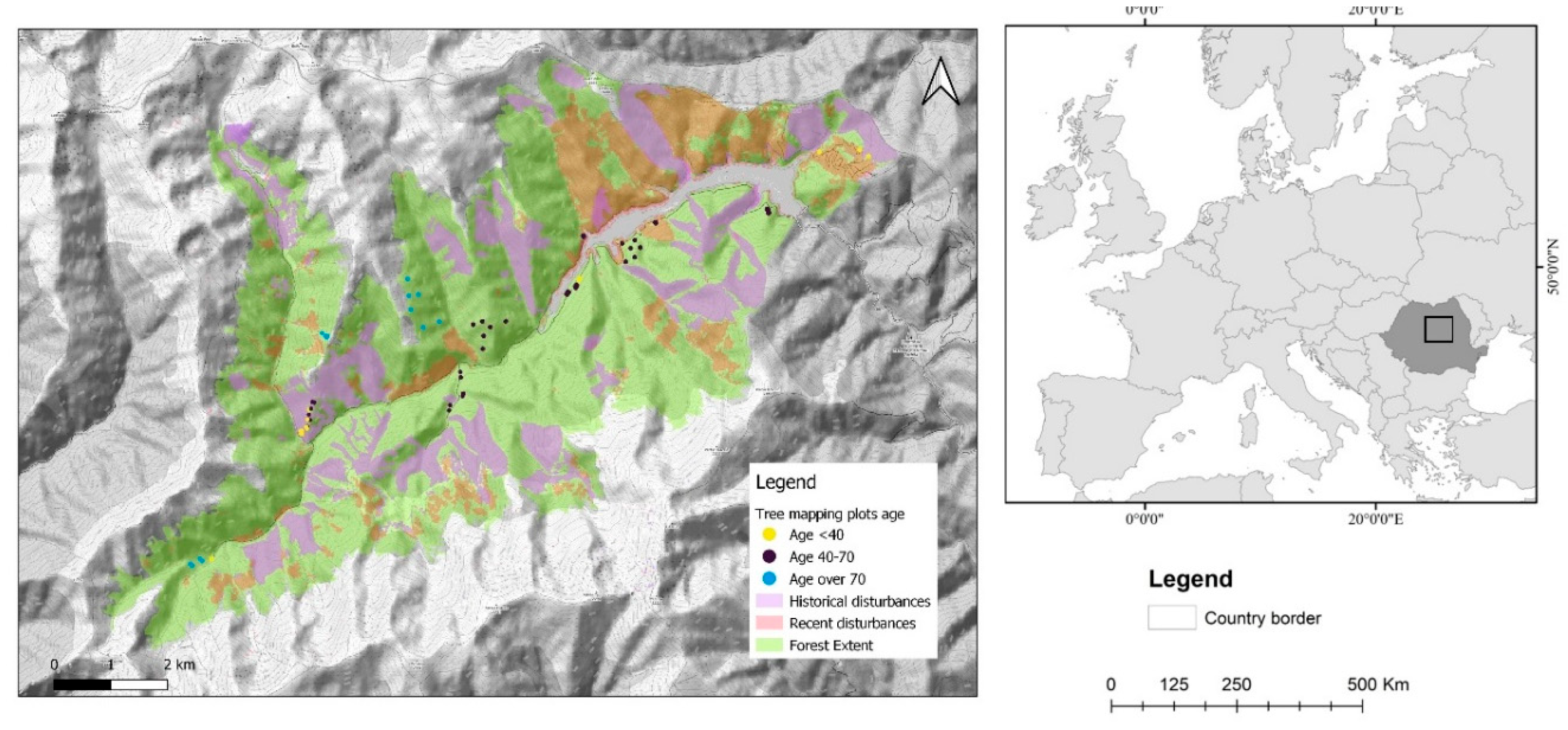
Figure 2.
Workflow and example of tree inventory dataset for a plot.
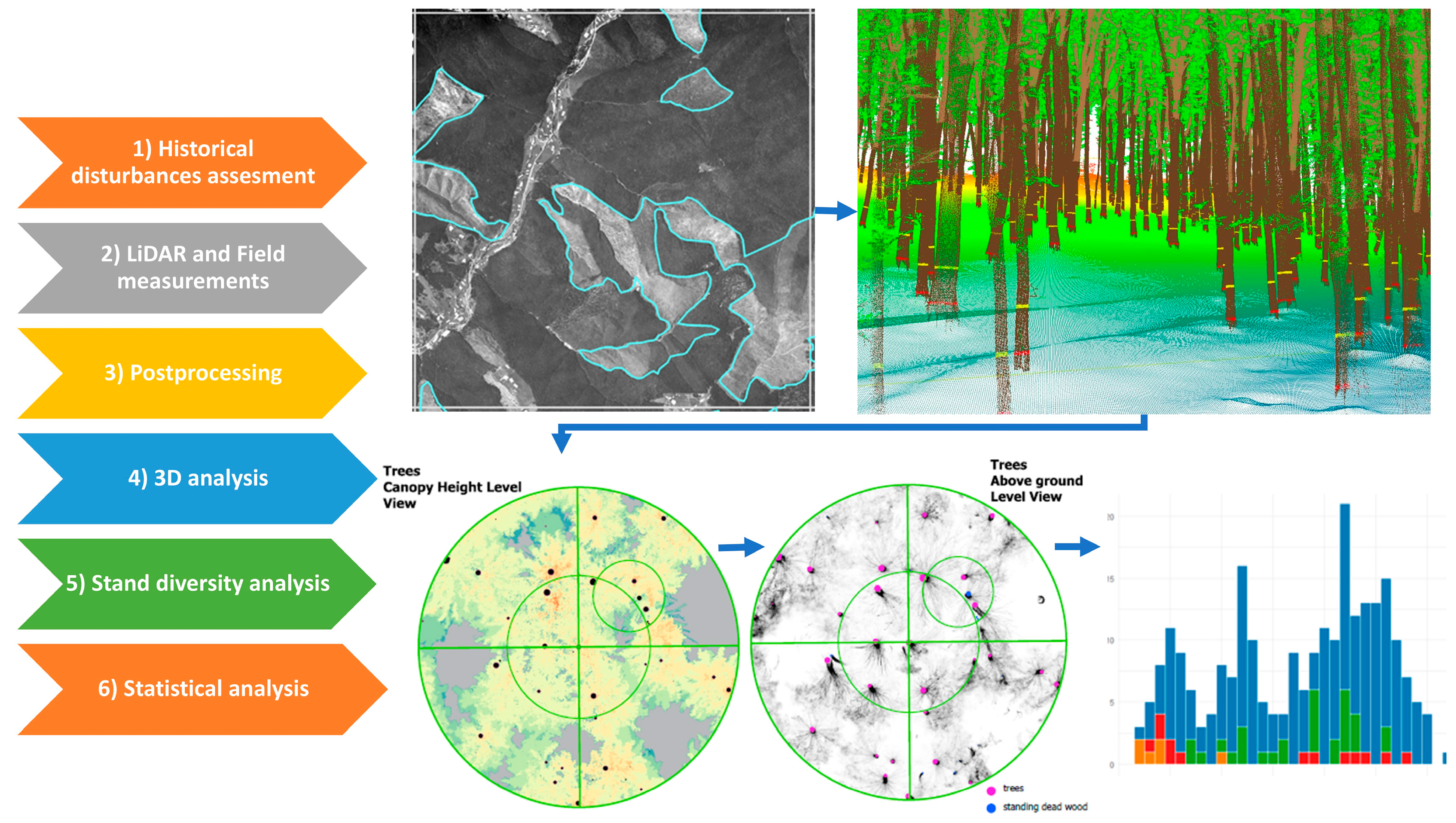
Figure 4.
Structural differentiation vs. Disturbance age.
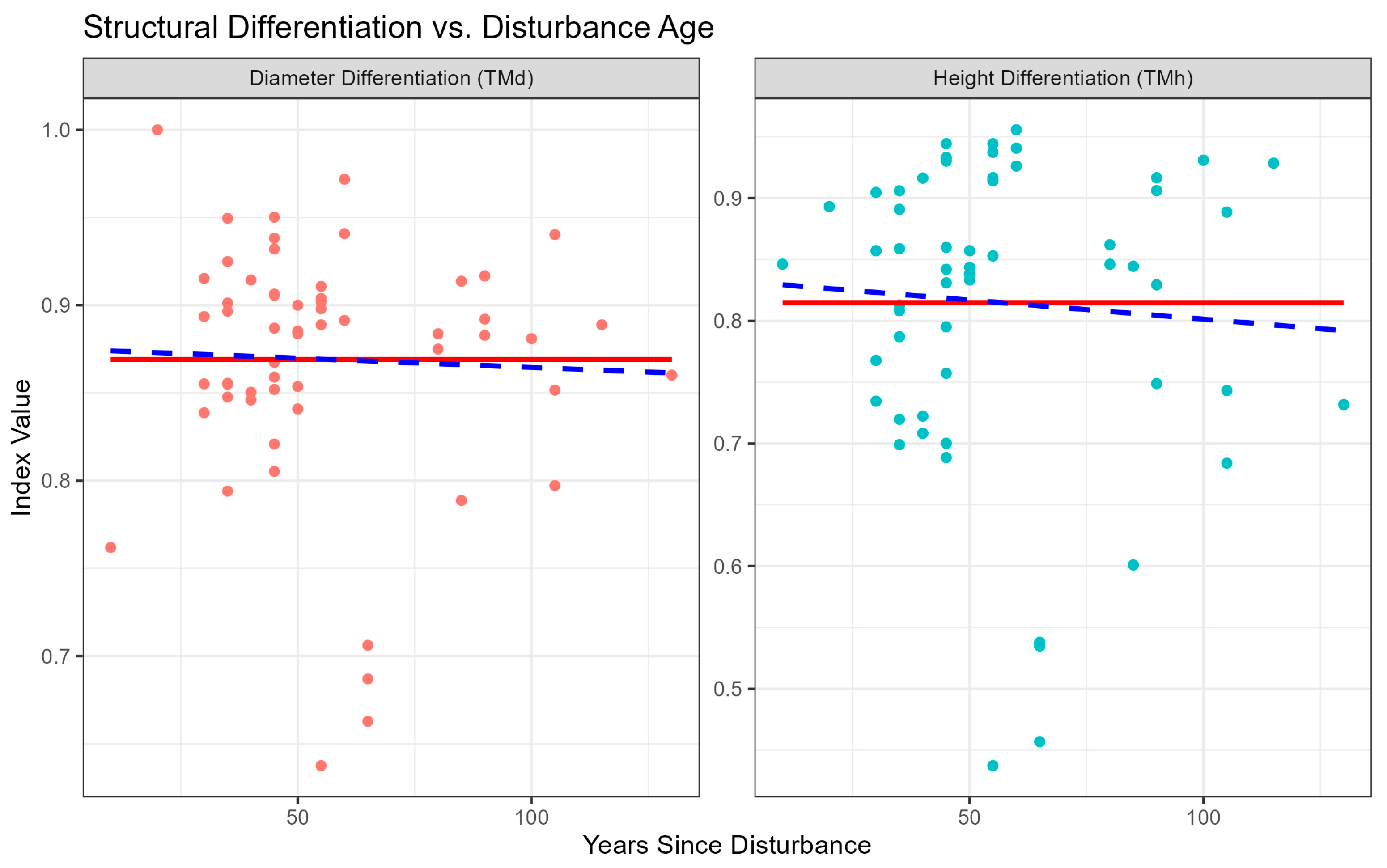
Figure 5.
Composite Diversity vs. disturbance age.
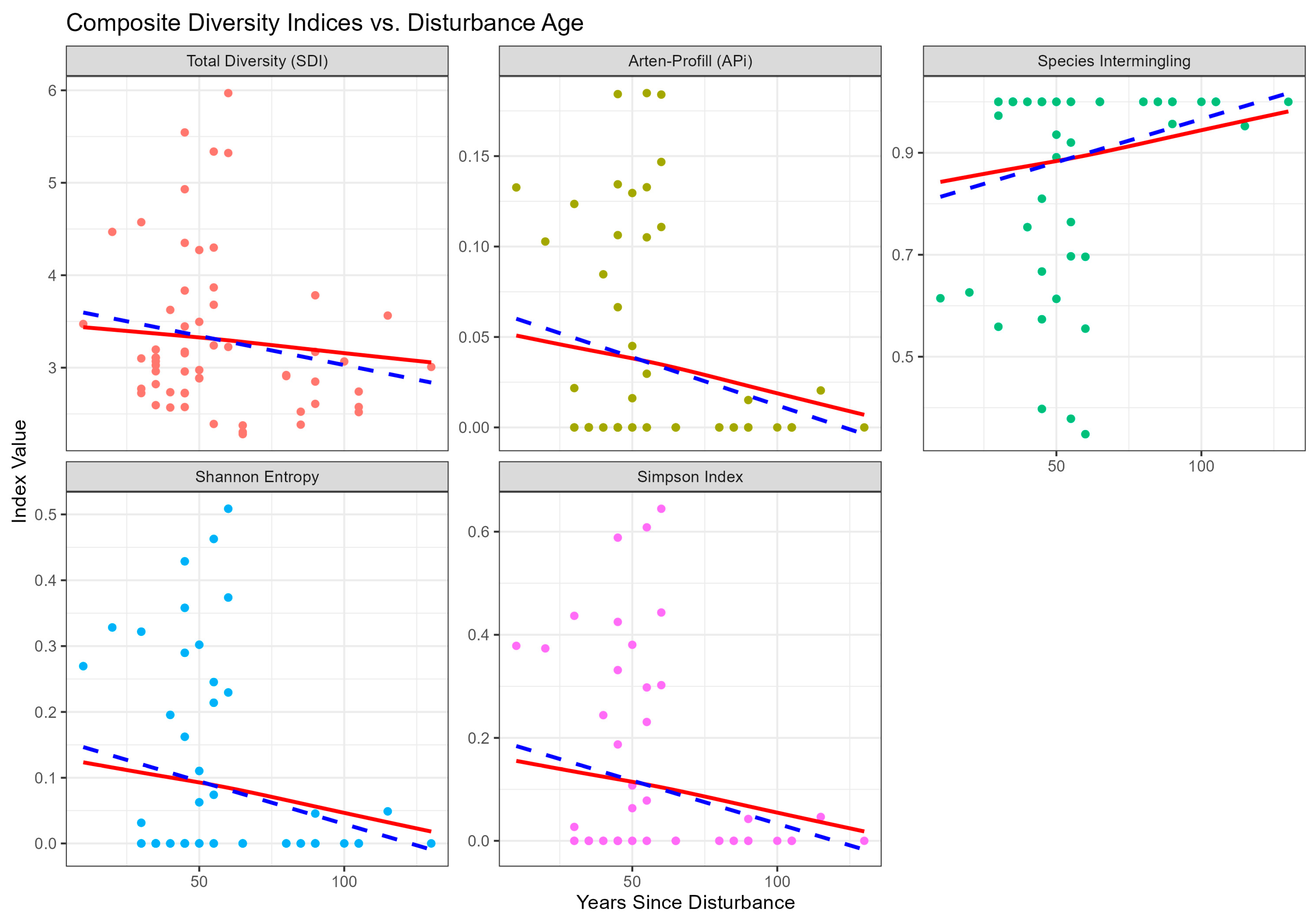
Figure 6.
Comparison Volume per hectare, Richness, Stand Diversity Index, Basal Area by Origin and disturbance.
Figure 6.
Comparison Volume per hectare, Richness, Stand Diversity Index, Basal Area by Origin and disturbance.
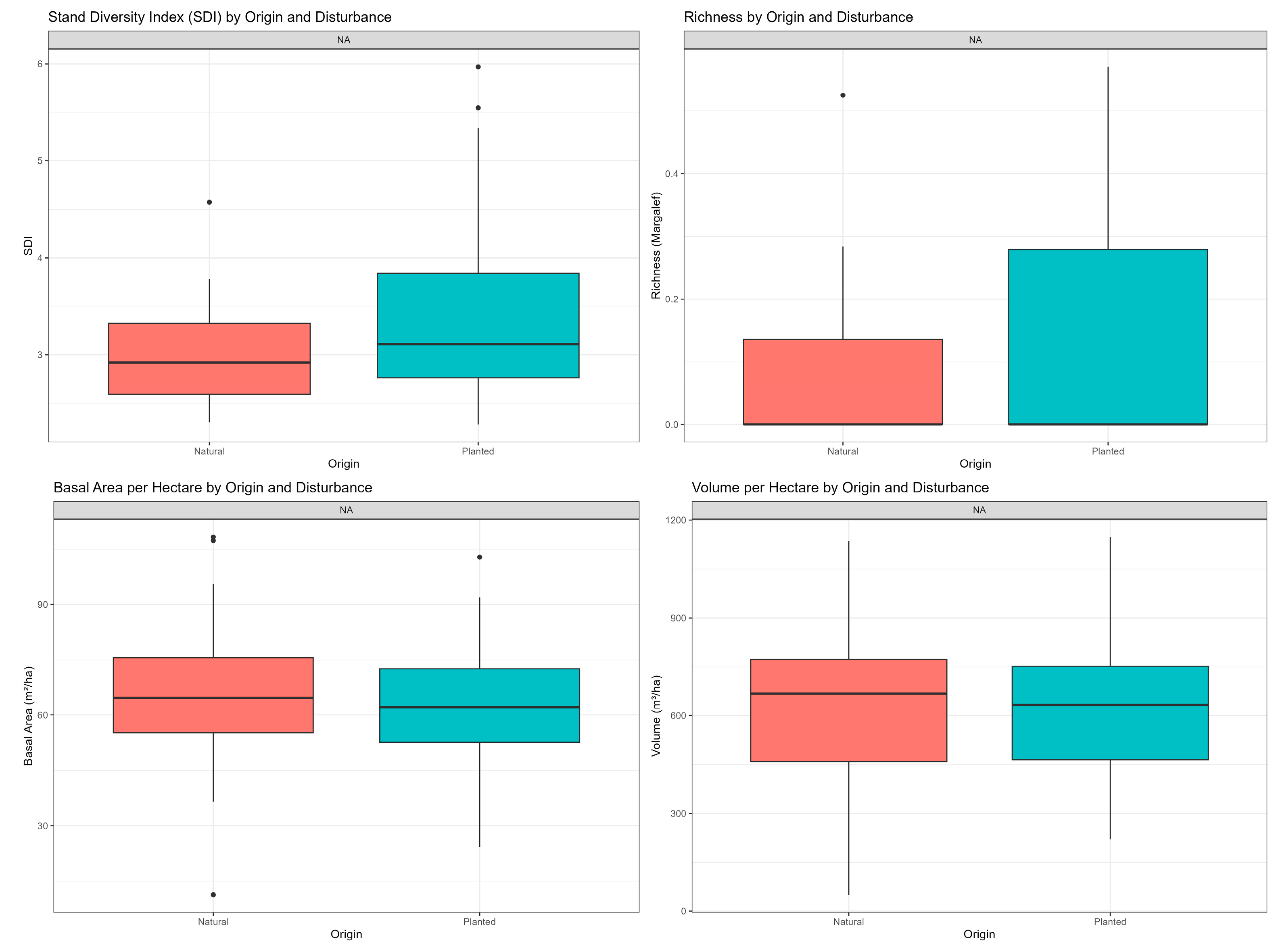
Figure 7.
Principal Component Analysis of stand structural indexes and dendrogram hierarchical clustering of plots.
Figure 7.
Principal Component Analysis of stand structural indexes and dendrogram hierarchical clustering of plots.
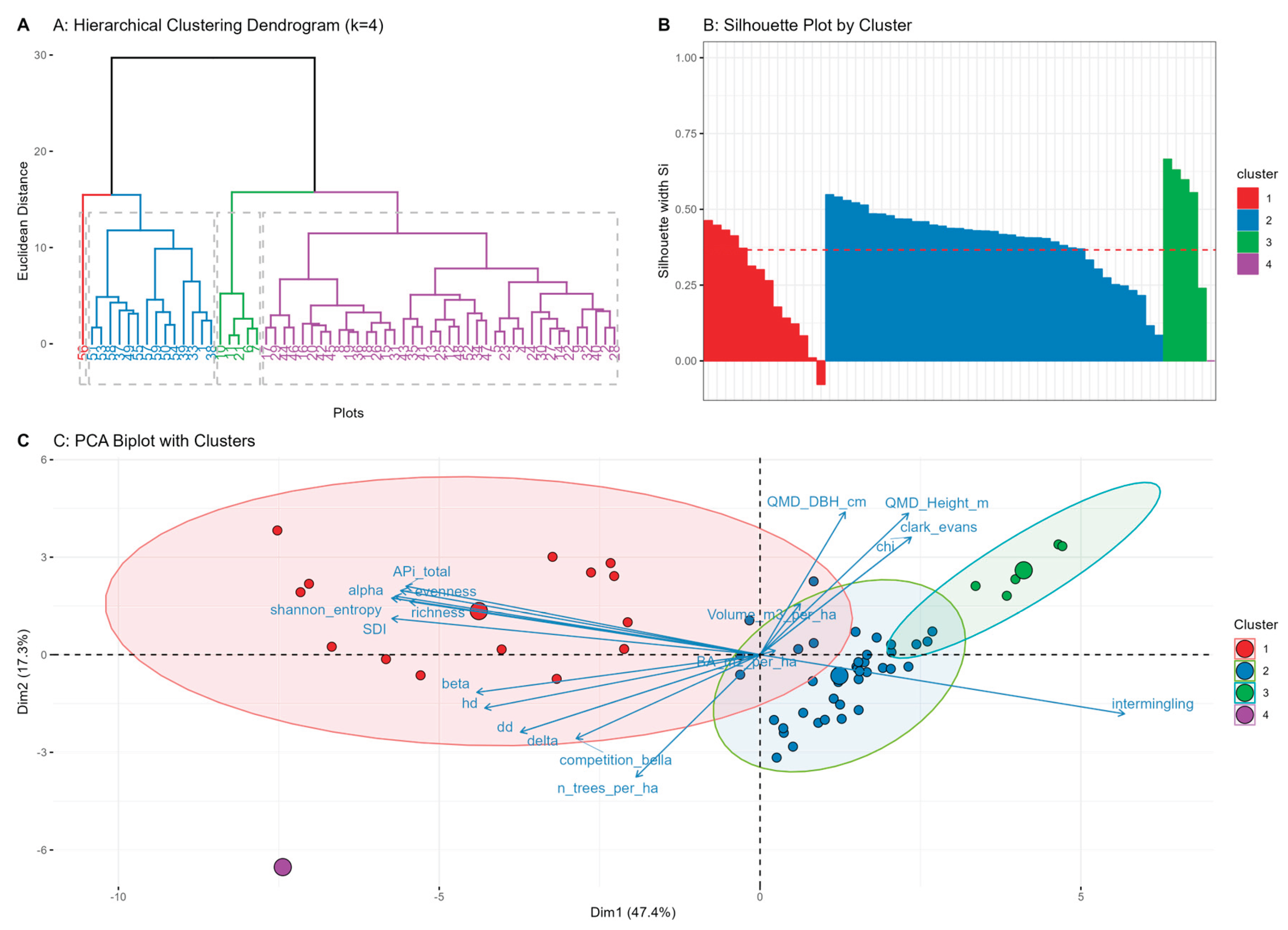

Table 1.
Spearman rank correlations between structural indices and time since disturbance (years).
| Index | Spearman_rho | p_value | significance |
|---|---|---|---|
| richness | -0.089490976 | 0.500285857 | ns |
| index_lambda | -0.100512116 | 0.448779967 | ns |
| shannon_entropy | -0.09872676 | 0.456919143 | ns |
| evenness | -0.099825441 | 0.4519009 | ns |
| clark_evans | -0.065165784 | 0.62387927 | ns |
| dd | -0.022839889 | 0.863669297 | ns |
| hd | 0.036876525 | 0.781559178 | ns |
| intermingling | 0.100512116 | 0.448779967 | ns |
| competition_bella | -0.195556141 | 0.137721599 | ns |
| alpha | -0.09872676 | 0.456919143 | ns |
| beta | -0.04914623 | 0.711646388 | ns |
| chi | -0.065165784 | 0.62387927 | ns |
| delta | -0.022839889 | 0.863669297 | ns |
| APi_total | -0.091001661 | 0.493050198 | ns |
| SDI | -0.180829908 | 0.170502416 | ns |
| n_trees_per_ha | -0.382294178 | 0.002807859 | ** |
| QMD_DBH_cm | 0.620882664 | 1.5524E-07 | *** |
| QMD_Height_m | 0.500368583 | 5.44673E-05 | *** |
| BA_m2_per_ha | 0.321390477 | 0.013062404 | * |
| Volume_m3_per_ha | 0.41259906 | 0.001164596 | ** |
Disclaimer/Publisher’s Note: The statements, opinions and data contained in all publications are solely those of the individual author(s) and contributor(s) and not of MDPI and/or the editor(s). MDPI and/or the editor(s) disclaim responsibility for any injury to people or property resulting from any ideas, methods, instructions or products referred to in the content. |
© 2026 by the authors. Licensee MDPI, Basel, Switzerland. This article is an open access article distributed under the terms and conditions of the Creative Commons Attribution (CC BY) license (http://creativecommons.org/licenses/by/4.0/).
Copyright: This open access article is published under a Creative Commons CC BY 4.0 license, which permit the free download, distribution, and reuse, provided that the author and preprint are cited in any reuse.