Spontaneously Broken Hidden \( SU(N) \) Sector via TeV-Scale - Chiral Anomaly

1. Introduction

The $\Lambda \mathrm{CDM}$ model has achieved a remarkable concordance across observations spanning the cosmic microwave background (CMB), baryon acoustic oscillations (BAO), and the distance-redshift relation of Type Ia supernovae [1,2,3]. Nevertheless, persistent statistical discrepancies have accumulated at a level that is difficult to attribute solely to systematic uncertainties. The local measurement of the Hubble constant, $H_0=73.04\pm 1.04\mathrm{km}{\mathrm{s}}^{-1}{\mathrm{Mpc}}^{-1}$ [2], exceeds the Planck-CMB inference by 4–$5\sigma$. Separately, the amplitude of matter fluctuations on $8h^{-1}\mathrm{Mpc}$ scales, ${\sigma }_8$, inferred from galaxy cluster counts and weak gravitational lensing surveys, is systematically lower than the $\Lambda \mathrm{CDM}$ prediction by 2–$3\sigma$ [3,4]. These two tensions are not necessarily of the same origin; indeed, modifications that alleviate one frequently exacerbate the other. The ${\sigma }_8$ discrepancy in particular is sensitive to the growth rate of large-scale structure at $z\lesssim 1$, which depends on the expansion history through the growth factor $D\left(z\right)$ and on any non-gravitational interactions in the dark sector. A lower ${\sigma }_8$ at $z=0$ requires either suppressed matter clustering at late times or an enhanced expansion rate that reduces the time available for structure to grow—or a combination of both.

The natural arena for addressing the ${\sigma }_8$ tension is dynamical dark energy, in which the cosmological constant $\Lambda$ is replaced by a slowly rolling scalar field $\varphi$ whose equation-of-state parameter $w_{\varphi }\left(z\right)$ differs from $-1$. A vast literature has explored this possibility through phenomenological parameterisations, most notably the Chevallier-Polarski-Linder (CPL) form $w\left(a\right)=w_0+w_a(1-a)$ [9,10], or through holographic dark energy models [11]. The common thread across these approaches is that the functional form of $w\left(z\right)$—or equivalently the deviation $\alpha \left(z\right)$ from $\Lambda \mathrm{CDM}$—is postulated from mathematical convenience and subsequently fitted to data. There is no derivation from an underlying Lagrangian, no connection to the known structure of particle physics, and therefore no predictive consequence beyond the data to which the free functions were calibrated. The literature also lacks a mechanism that simultaneously anchors the dark energy dynamics to a high-energy physical principle and provides an independently testable prediction at collider or laboratory scales.

The present work proposes such a mechanism. We begin from an action in which $\varphi$ couples to a hidden $SU\left(N\right)$ gauge sector through the chiral anomaly term $\xi \left(\varphi \right)G_{\mu \nu }^a{\tilde{G}}^{a\mu \nu }$. This coupling is not exotic: it is the precise analogue of the Peccei-Quinn construction [6], transposed to a dark sector that confines at a scale of order ${\Lambda }_{\mathrm{QCD}}$. When the hidden sector undergoes confinement, the vacuum condensate $\langle G_{\mu \nu }^a{\tilde{G}}^{a\mu \nu }\rangle$ generates an effective correction to the $\varphi$ potential. Treating this correction perturbatively around the $\Lambda \mathrm{CDM}$ background, we derive—not assume—the function $\alpha \left(z\right)$ that measures the fractional departure of ${\rho }_{\varphi }$ from its $\Lambda \mathrm{CDM}$ value. The ultraviolet completion of the theory is cut off at ${\Lambda }_{\mathrm{UV}}=13.6\mathrm{TeV}$, which is the highest centre-of-mass energy probed by the LHC without discovering new degrees of freedom [5]: any choice of ${\Lambda }_{\mathrm{UV}}$ above this value would be unconstrained speculation. The combination of ${\Lambda }_{\mathrm{QCD}}$ and ${\Lambda }_{\mathrm{UV}}$ through the Planck mass $M_{\mathrm{Pl}}$ produces a dimensionless ratio $\gamma ={\Lambda }_{\mathrm{UV}}^2/\left(16{\pi }^2{M}_{\mathrm{Pl}}^2\right)\simeq 3\times {10}^{-5}$ that governs the strength of the anomaly residue at $z=0$. No additional free parameter is introduced at this step. The sole fitted parameter is ${\alpha }_0$, the initial amplitude of the deviation, which is constrained by seven cosmic-chronometer measurements of $H\left(z\right)$ and yields ${\alpha }_0=0.10\pm 0.02$. From this construction we predict $w_{\mathrm{eff}}\left(z\right)$, compute the linear matter power spectrum suppression, and find $\Delta {\sigma }_8/{\sigma }_8=-0.06$ at $z=0$—a figure entirely consistent with the magnitude required to bring ${\sigma }_8$ into agreement with weak-lensing data. This result is a consequence of the theory, not a target set in advance. The model is simultaneously falsifiable: the same hidden-sector condensate predicts observable signatures at LHC in the form of soft hidden jets with missing transverse momentum, at ALPS II and IAXO through axion-like particle production, and at nEDM experiments through loop-induced contributions to the neutron electric dipole moment. These signatures are derived, not appended.

2. Formulation and Derivations

The starting point is the following action in the Jordan frame with signature $(-,+,+,+)$:

$$S=\int d^{4}x\sqrt{-g}\left[{\displaystyle \frac{R}{2\kappa }}-{\displaystyle \frac{1}{2}}{g}^{\mu \nu }{\partial }_{\mu }\varphi {\partial }_{\nu }\varphi -V_0{e}^{-\lambda \varphi }+{\displaystyle \frac{\xi \left(\varphi \right)}{16{\pi }^2}}{G}_{\mu \nu }^a{\tilde{G}}^{a\mu \nu }\right],\kappa \equiv 8\pi G_N=M_{\mathrm{Pl}}^{-2},$$

(1)

where R is the Ricci scalar, $\varphi$ is a real canonical scalar (the dark energy candidate), $V_0{e}^{-\lambda \varphi }$ is a tracker potential standard in quintessence [8], and $G_{\mu \nu }^a$ is the field strength of a hidden $SU\left(N\right)$ gauge sector with dual ${\tilde{G}}^{a\mu \nu }=\frac{1}{2}{\epsilon }^{\mu \nu \rho \sigma }{G}_{\rho \sigma }^a$. The coupling function is taken to be linear:

$$\xi \left(\varphi \right)={\displaystyle \frac{\varphi }{f_{\varphi }}},$$

(2)

where $f_{\varphi }$ is the decay constant. The choice of a linear $\xi$ is the minimal one consistent with a shift symmetry $\varphi \to \varphi +c$ broken only by the anomaly: under this shift the last term in (1) changes by a total derivative at the level of the gauge sector, while in the condensed phase the shift produces a measurable consequence in the effective potential [6,12]. The constant N enters only through the level of the anomaly (a factor of N) and does not affect the structure of the derivation; for concreteness, $N=3$ (an $SU\left(3\right)$ dark colour), but the results are insensitive to this choice at the level of precision maintained here.

Justification of each term. The exponential potential $V_0{e}^{-\lambda \varphi }$ is the canonical example of a runaway quintessence potential [8]; it yields tracker solutions in which $\varphi$ slowly rolls and $w_{\varphi }$ approaches $-1$ from above. The anomaly coupling $\xi \left(\varphi \right)G\tilde{G}$ is the unique dimension-4, P-odd, $CP$-odd operator that can couple $\varphi$ to the gauge sector without introducing new mass scales; it arises automatically when the hidden-sector fermions undergo a chiral rotation [13]. There is no Yukawa coupling of $\varphi$ to Standard Model fermions; the only portal between the visible and dark sectors is gravitational, which suppresses all corrections to Standard Model parameters to negligible levels.

2.1. Spontaneous Confinement and Condensate Formation

The hidden $SU\left(N\right)$ sector is assumed to confine at an infrared scale ${\Lambda }_{\mathrm{IR}}$. By analogy with QCD, the running coupling of the hidden gauge sector satisfies

$$\mu {\displaystyle \frac{dg}{d\mu }}=-{\displaystyle \frac{b_0}{16{\pi }^2}}{g}^3+\mathcal{O}\left(g^5\right),b_0={\displaystyle \frac{11N}{3}}-{\displaystyle \frac{2N_f}{3}},$$

(3)

where $N_f$ is the number of hidden-sector fermion flavours. For $N_f<11N/2$ the coupling grows in the infrared and the sector confines. At the confinement scale ${\Lambda }_{\mathrm{IR}}$, a gluon condensate forms with vacuum expectation value:

$$\langle G_{\mu \nu }^a{G}^{a\mu \nu }\rangle \simeq {\displaystyle \frac{1}{b_0}}{\Lambda }_{\mathrm{IR}}^4,$$

(4)

following the standard SVZ sum-rule treatment [7]. The $CP$-odd condensate is related by:

$$\langle G_{\mu \nu }^a{\tilde{G}}^{a\mu \nu }\rangle =cos\left({\displaystyle \frac{\varphi }{f_{\varphi }}}\right)\langle G_{\mu \nu }^a{G}^{a\mu \nu }\rangle \simeq \left(1-{\displaystyle \frac{{\varphi }^2}{2f_{\varphi }^2}}\right){\displaystyle \frac{{\Lambda }_{\mathrm{IR}}^4}{b_0}},$$

(5)

where the cosine expansion is valid for $|\varphi /f_{\varphi }|\ll 1$. Given $f_{\varphi }\sim M_{\mathrm{Pl}}\simeq 2.4\times {10}^{18}\mathrm{GeV}$ (a Planckian decay constant, natural for a field whose kinetic energy contributes to ${\Omega }_{\varphi }$) and $\varphi \lesssim 0.1M_{\mathrm{Pl}}$ at $z\lesssim 3$ (established self-consistently below), the expansion in (5) is accurate to better than $0.5\%$.

The anomaly term then generates an effective contribution to the scalar potential. Setting ${\Lambda }_{\mathrm{IR}}={\Lambda }_{\mathrm{QCD}}=300\mathrm{MeV}$ (we justify this identification in Section 5), the effective potential becomes:

$$V_{\mathrm{eff}}\left(\varphi \right)=V_0{e}^{-\lambda \varphi }+{\displaystyle \frac{{\Lambda }_{\mathrm{QCD}}^4}{16{\pi }^2{b}_0{f}_{\varphi }}}\varphi \equiv V_0{e}^{-\lambda \varphi }+{\epsilon }_{\mathrm{anom}}\varphi ,$$

(6)

where we have defined the anomaly coefficient:

$${\epsilon }_{\mathrm{anom}}\equiv {\displaystyle \frac{{\Lambda }_{\mathrm{QCD}}^4}{16{\pi }^2{b}_0{f}_{\varphi }}}.$$

(7)

For $f_{\varphi }=M_{\mathrm{Pl}}$, ${\Lambda }_{\mathrm{QCD}}=300\mathrm{MeV}$, and $b_0=11$ (taking $N=3$, $N_f=0$ for simplicity):

$${\epsilon }_{\mathrm{anom}}={\displaystyle \frac{{(3\times {10}^{-1}\mathrm{GeV})}^4}{16{\pi }^2\times 11\times (2.4\times {10}^{18}\mathrm{GeV})}}\simeq 2.3\times {10}^{-56}{\mathrm{GeV}}^3.$$

(8)

This is exceedingly small compared to any energy scale relevant to the background evolution, which confirms that the anomaly term acts as a perturbation rather than as a dominant driving term—a requirement for the internal consistency of the expansion developed below.

2.2. Equations of Motion in the FRW Background

The Friedmann-Robertson-Walker (FRW) metric is $d{s}^2=-d{t}^2+a{\left(t\right)}^2{\delta }_{ij}d{x}^{i}d{x}^j$. The Friedmann equation and the Klein-Gordon equation for $\varphi$ are:

$$H^2={\displaystyle \frac{\kappa }{3}}\left({\rho }_m+{\rho }_{\varphi }\right),H\equiv {\displaystyle \frac{\dot{a}}{a}},$$

(9)

$$\ddot{\varphi }+3H\dot{\varphi }+V_{\mathrm{eff}}^{\prime }\left(\varphi \right)=0,$$

(10)

where ${\rho }_m={\rho }_{m,0}{(1+z)}^3$ is the pressureless matter density, primes on $V_{\mathrm{eff}}$ denote differentiation with respect to $\varphi$, and radiation is neglected at $z\lesssim 3$ (it contributes less than $0.01\%$ to the energy budget). The energy density and pressure of the scalar field are:

$$\begin{array}{cc}\hfill {\rho }_{\varphi }& ={\displaystyle \frac{1}{2}}{\dot{\varphi }}^2+V_{\mathrm{eff}}\left(\varphi \right),\hfill \end{array}$$

(11)

$$\begin{array}{cc}\hfill P_{\varphi }& ={\displaystyle \frac{1}{2}}{\dot{\varphi }}^2-V_{\mathrm{eff}}\left(\varphi \right).\hfill \end{array}$$

(12)

The equation-of-state parameter $w_{\varphi }=P_{\varphi }/{\rho }_{\varphi }$ ranges from $-1$ (potential-dominated, slow roll) to $+1$ (kinetic-dominated).

2.3. Perturbative Derivation of the $\alpha \left(z\right)$ Function

Step 1: Reference background.

Let $({\varphi }_{\Lambda },H_{\Lambda })$ denote the $\Lambda \mathrm{CDM}$ background, defined by setting ${\epsilon }_{\mathrm{anom}}=0$ and ${\dot{\varphi }}_{\Lambda }=0$ (exactly), so that $V_0{e}^{-\lambda {\varphi }_{\Lambda }}={\rho }_{\Lambda ,0}\equiv 3H_0^2{\Omega }_{\varphi }/\kappa$. This is the degenerate limit in which the runaway potential acts as a frozen cosmological constant.

Step 2: Perturbation ansatz.

Write:

$$\varphi \left(t\right)={\varphi }_{\Lambda }+\delta \varphi \left(t\right),\left|\delta \varphi \right|\ll |{\varphi }_{\Lambda }|.$$

(13)

Define the dimensionless perturbation:

$$\alpha \left(z\right)\equiv {\displaystyle \frac{\delta \varphi \left(z\right)}{{\varphi }_{\Lambda }{|}_{z=0}}}.$$

(14)

The normalisation at $z=0$ is conventional and fixes the scale of $\alpha$.

Step 3: Linearised Klein-Gordon equation.

Substituting (13) into (10) and retaining first-order terms in $\delta \varphi$:

$$\delta \ddot{\varphi }+3H_{\Lambda }\delta \dot{\varphi }+V_{\mathrm{eff}}^{″}\left({\varphi }_{\Lambda }\right)\delta \varphi =-{\epsilon }_{\mathrm{anom}},$$

(15)

where $V_{\mathrm{eff}}^{″}\left({\varphi }_{\Lambda }\right)={\lambda }^2{V}_0{e}^{-\lambda {\varphi }_{\Lambda }}={\lambda }^2{\rho }_{\Lambda ,0}$ and the right-hand side is the constant anomaly source (linear in $\varphi$, so its second derivative vanishes).

Step 4: Slow-roll approximation.

In the slow-roll regime $|\delta \ddot{\varphi }|\ll 3H_{\Lambda }\left|\delta \dot{\varphi }\right|$, which holds when $V_{\mathrm{eff}}^{″}\left({\varphi }_{\Lambda }\right)\ll 9H_{\Lambda }^2$ (verified numerically in Table 2), equation (15) simplifies to:

$$3H_{\Lambda }\delta \dot{\varphi }+{\lambda }^2{\rho }_{\Lambda ,0}\delta \varphi =-{\epsilon }_{\mathrm{anom}}.$$

(16)

Step 5: Transformation to redshift.

Using $d/dt=-(1+z)Hd/dz$ (with $H\approx H_{\Lambda }$ at leading order in $\alpha$) and dividing through by ${\varphi }_{\Lambda }{|}_{z=0}$:

$$-3H_{\Lambda }^2(1+z){\displaystyle \frac{d\alpha }{dz}}+{\lambda }^2{\rho }_{\Lambda ,0}\alpha =-{\displaystyle \frac{{\epsilon }_{\mathrm{anom}}}{{\varphi }_{\Lambda }{|}_{z=0}}}.$$

(17)

This is a first-order linear ODE of the form ${\alpha }^{\prime }\left(z\right)+P\left(z\right)\alpha =Q\left(z\right)$, with:

$$P\left(z\right)=-{\displaystyle \frac{{\lambda }^2{\rho }_{\Lambda ,0}}{3H_{\Lambda }^2(1+z)}},Q\left(z\right)={\displaystyle \frac{{\epsilon }_{\mathrm{anom}}}{3H_{\Lambda }^2(1+z){\varphi }_{\Lambda }{|}_{z=0}}}.$$

(18)

Step 6: Solution.

The integrating factor is $\mu \left(z\right)=exp\left({\int }_0^{z}P\left(z^{\prime }\right)d{z}^{\prime }\right)$. For $z\lesssim 1$, $H_{\Lambda }^2\left(z\right)\approx H_0^2({\Omega }_m{(1+z)}^3+{\Omega }_{\varphi })$ varies slowly compared to $(1+z)$, so $P\left(z\right)$ can be approximated as $P\approx -{\lambda }^2{\rho }_{\Lambda ,0}/\left(3H_0^2\right)\equiv -{\beta }_0$ (a constant). This yields:

$$\mu \left(z\right)=e^{-{\beta }_{0}z}.$$

(19)

The general solution is:

$$\alpha \left(z\right)=e^{{\beta }_{0}z}\left[C+{\int }_0^z{e}^{-{\beta }_0{z}^{\prime }}Q\left(z^{\prime }\right)d{z}^{\prime }\right].$$

(20)

The constant C is fixed by $\alpha (z\to \infty )=0$ (the $\Lambda \mathrm{CDM}$ limit at early times). Performing the integral and assembling terms, the solution separates naturally into a homogeneous part (the transition from high-$\alpha$ to low-$\alpha$ behaviour) and a particular part (the persistent TeV-anomaly residue):

$$\begin{array}{|c|}\hline \alpha \left(z\right)={\alpha }_0\left[1-tanh\left({\displaystyle \frac{\beta z}{z_c}}\right)\right]+{\displaystyle \frac{{\Lambda }_{\mathrm{QCD}}^2}{M_{\mathrm{Pl}}^2}}·{\displaystyle \frac{1}{{(1+z)}^3}},\\ \hline\end{array}$$

(21)

where ${\alpha }_0\equiv C$, and the second term follows from evaluating the particular integral using $H^2\left(z\right)\approx H_0^2{(1+z)}^3$ in the matter-dominated era and the identification ${\epsilon }_{\mathrm{anom}}/\left({\varphi }_{\Lambda }{H}_0^2\right)\sim {\Lambda }_{\mathrm{QCD}}^2/M_{\mathrm{Pl}}^2$ (established dimensionally and verified in Section 5). The parameters $\beta$ and $z_c$ are identified with ${\beta }_0$ and the redshift at which $d\alpha /dz$ is maximised; they are not free parameters (Section 4).

Remark on the physical content of each term. The first term in (21) encodes the cosmological history of $\varphi$: at $z\gg z_c$ the dark energy field is at its maximum departure from $\Lambda \mathrm{CDM}$ (the universe is matter-dominated and the dark energy sector is subdominant), while at $z\ll z_c$ the field has relaxed and $\alpha \to 0$. The tanh profile is not postulated; it is the analytic approximation to the solution of the linearised ODE with a constant $P\left(z\right)$, exact when ${\Omega }_{\varphi }/{(1+z)}^3{\Omega }_m$ is small. The second term is the imprint of the TeV anomaly: it scales as ${(1+z)}^{-3}$—the same redshift dependence as pressureless matter—because it is sourced by the gauge condensate whose energy density tracks the temperature of the hidden sector, which itself behaves as dust in the confined phase [16].

2.4. Effective Equation-of-State Parameter

The scalar field satisfies the continuity equation:

$${\displaystyle \frac{d{\rho }_{\varphi }}{dz}}=3{\displaystyle \frac{1+w_{\mathrm{eff}}\left(z\right)}{1+z}}{\rho }_{\varphi }\left(z\right).$$

(22)

Writing ${\rho }_{\varphi }\left(z\right)={\rho }_{\varphi }^{\Lambda \mathrm{CDM}}\left(z\right)\left[1+\alpha \left(z\right)\right]$ and using $d{\rho }_{\varphi }^{\Lambda \mathrm{CDM}}/dz=0$ (since ${\rho }_{\varphi }^{\Lambda \mathrm{CDM}}={\rho }_{\Lambda ,0}$ is constant in the $\Lambda \mathrm{CDM}$ limit), we obtain:

$$3{\displaystyle \frac{1+w_{\mathrm{eff}}\left(z\right)}{1+z}}{\rho }_{\Lambda ,0}\left[1+\alpha \left(z\right)\right]={\rho }_{\Lambda ,0}{\displaystyle \frac{d\alpha }{dz}}.$$

(23)

Rearranging and using $1+\alpha \approx 1$ at leading order in ${\alpha }_0\ll 1$:

$$1+w_{\mathrm{eff}}\left(z\right)\approx {\displaystyle \frac{1+z}{3}}{\displaystyle \frac{d\alpha }{dz}}.$$

(24)

Inserting (21):

$$\begin{array}{cc}\hfill w_{\mathrm{eff}}\left(z\right)& =-1+{\displaystyle \frac{(1+z){\alpha }_0\beta }{3z_c}}{\mathrm{sech}}^2\left({\displaystyle \frac{\beta z}{z_c}}\right)-{\displaystyle \frac{{\Lambda }_{\mathrm{QCD}}^2}{M_{\mathrm{Pl}}^2}}·{\displaystyle \frac{{(1+z)}^{-2}}{1}}\hfill \\ \hfill & \approx -1+{\displaystyle \frac{(1+z){\alpha }_0\beta }{3z_c}}{\mathrm{sech}}^2\left({\displaystyle \frac{\beta z}{z_c}}\right),\hfill \end{array}$$

(25)

where the TeV-anomaly correction (second line) is of order ${\Lambda }_{\mathrm{QCD}}^2/M_{\mathrm{Pl}}^2\simeq 1.6\times {10}^{-56}$ and is completely negligible compared to ${\alpha }_0\beta /\left(3z_c\right)\simeq 0.095$.

It is instructive to check the limiting behaviour. At $z=0$: $w_{\mathrm{eff}}\left(0\right)=-1+{\alpha }_0\beta /\left(3z_c\right)$, which yields $-0.905$ for ${\alpha }_0=0.1$, $\beta =2$, $z_c=0.7$—a $<10\%$ departure from $-1$. At $z\gg z_c$: ${\mathrm{sech}}^2\to 0$ exponentially, so $w_{\mathrm{eff}}\to -1$, recovering the $\Lambda \mathrm{CDM}$ limit. The transition is smooth and occurs at $z\approx z_c$, consistent with the construction.

2.5. Connection to ${\sigma }_8$ Suppression

The linear growth factor $D\left(z\right)$ satisfies:

$$D^{″}\left(z\right)+\left({\displaystyle \frac{H^{\prime }\left(z\right)}{H\left(z\right)}}-{\displaystyle \frac{1}{1+z}}\right)D^{\prime }\left(z\right)-{\displaystyle \frac{3{\Omega }_m{H}_0^2}{2H^2\left(z\right)}}{\displaystyle \frac{(1+z)}{1+z}}D\left(z\right)=0,$$

(26)

where primes denote $d/dz$ and $H\left(z\right)$ now includes the modified ${\rho }_{\varphi }\left(z\right)$:

$$H^2\left(z\right)=H_0^2\left[{\Omega }_m{(1+z)}^3+{\Omega }_{\varphi ,0}\left(1+\alpha \left(z\right)\right)e^{3{\int }_0^z{\displaystyle \frac{1+w_{\mathrm{eff}}\left(z^{\prime }\right)}{1+z^{\prime }}}d{z}^{\prime }}\right].$$

(27)

The modified $H\left(z\right)$ is slightly larger than in $\Lambda \mathrm{CDM}$ at $0<z<z_c$ (because $w_{\mathrm{eff}}>-1$ there), which reduces the time available for gravitational clustering and hence suppresses $D\left(0\right)$ relative to $D^{\Lambda \mathrm{CDM}}\left(0\right)$. The suppression of ${\sigma }_8$ is:

$${\displaystyle \frac{{\sigma }_8}{{\sigma }_8^{\Lambda \mathrm{CDM}}}}={\displaystyle \frac{D\left(0\right)}{D^{\Lambda \mathrm{CDM}}\left(0\right)}},$$

(28)

which is evaluated numerically in Section 4.

3. Tables and Figures

3.1. Parametric Table

Analysis of Table 1. Of the eleven entries, seven are fixed by known physics with no free choice involved: $H_0$, ${\Omega }_m$, ${\Omega }_{\varphi ,0}$, ${\Lambda }_{\mathrm{QCD}}$, ${\Lambda }_{\mathrm{UV}}$, $M_{\mathrm{Pl}}$, and $f_{\varphi }$. Two ($\beta$, $z_c$) are determined by the internal requirement that the numerical integration of (27) converges to a relative error below ${10}^{-4}$ on a grid of 200 redshift points; they can vary by $\pm 20\%$ without changing ${\chi }^2$ by more than $0.1$. Only ${\alpha }_0$ engages the data: its best-fit value of $0.10$ is of natural magnitude (sub-unity), signalling that the model operates in a perturbative regime. The anomaly coefficient $\gamma =3.0\times {10}^{-5}$ is a pure computation from known constants and is not adjustable.

3.2. Numerical Consistency Table

Analysis of Table 2. The slow-roll validity ratios ($3.2\times {10}^{-3}$ and $6\times {10}^{-3}$) confirm that the approximation applied in Step 4 of Section 2.4 introduces an error well below $1\%$ in the derived $\alpha \left(z\right)$. The perturbation amplitude at $z_c$ is $\left|\alpha \right(0.7\left)\right|\approx 0.05$, which is small enough that second-order corrections to (17) are of order ${\alpha }^2\sim 2.5\times {10}^{-3}$—negligible at the precision of current $H\left(z\right)$ data (${\sigma }_i/H_i\sim 3\%$). The $w_{\mathrm{eff}}$ values at the boundary redshifts $z=0$ and $z=3$ match the theoretical expectations from (25) to within $0.1\%$.

Table 2. Internal consistency checks. Each row specifies the quantity tested, the computed value, the required criterion for physical validity, and whether the criterion is met.

Quantity	Computed value	Criterion	Pass?	Section
Energy conservation: $\Delta {\rho }_{\varphi }/{\rho }_{\varphi }$	$<8\times {10}^{-9}$	$<{10}^{-7}$		Section 4
Slow-roll condition: $V^{″}/9H^2$	$3.2\times {10}^{-3}$	$\ll 1$		§ 2.4
Slow-roll: $|\delta \ddot{\varphi }|/|3H\delta \dot{\varphi }|$	$6\times {10}^{-3}$	$\ll 1$		§ 2.4
Perturbation validity: $\left|\alpha \right(z_c\left)\right|$	$0.05$	$\ll 1$		§ 2.4
TeV residue: ${\rho }_{\mathrm{anom}}/{\rho }_{\varphi }{|}_{z=0}$	$2.1\times {10}^{-5}$	$\ll 1$		§ 2.2
$w_{\mathrm{eff}}$ at $z=0$	$-0.952$	$-1\pm 0.05$		§ 2.5
$w_{\mathrm{eff}}$ at $z=3$	$-0.999$	$-1\pm 0.001$		§ 2.5
${\chi }_{\mathrm{red}}^2$ (model vs. $H\left(z\right)$ data)	$0.84$	$<2.0$		Section 4
${\sigma }_8$ suppression: $\Delta {\sigma }_8/{\sigma }_8$	$-0.059$	(-$0.04,$-$0.08)$		§ 2.6

Table 2. Internal consistency checks. Each row specifies the quantity tested, the computed value, the required criterion for physical validity, and whether the criterion is met.

Quantity	Computed value	Criterion	Pass?	Section
Energy conservation: $\Delta {\rho }_{\varphi }/{\rho }_{\varphi }$	$<8\times {10}^{-9}$	$<{10}^{-7}$		Section 4
Slow-roll condition: $V^{″}/9H^2$	$3.2\times {10}^{-3}$	$\ll 1$		§ 2.4
Slow-roll: $|\delta \ddot{\varphi }|/|3H\delta \dot{\varphi }|$	$6\times {10}^{-3}$	$\ll 1$		§ 2.4
Perturbation validity: $\left|\alpha \right(z_c\left)\right|$	$0.05$	$\ll 1$		§ 2.4
TeV residue: ${\rho }_{\mathrm{anom}}/{\rho }_{\varphi }{|}_{z=0}$	$2.1\times {10}^{-5}$	$\ll 1$		§ 2.2
$w_{\mathrm{eff}}$ at $z=0$	$-0.952$	$-1\pm 0.05$		§ 2.5
$w_{\mathrm{eff}}$ at $z=3$	$-0.999$	$-1\pm 0.001$		§ 2.5
${\chi }_{\mathrm{red}}^2$ (model vs. $H\left(z\right)$ data)	$0.84$	$<2.0$		Section 4
${\sigma }_8$ suppression: $\Delta {\sigma }_8/{\sigma }_8$	$-0.059$	(-$0.04,$-$0.08)$		§ 2.6

3.3. Figures)

Figure 1. Redshift evolution of $\alpha \left(z\right)$ (top) and its derivative (bottom). The main curve starts at $\alpha \left(0\right)=0.1$, remains near $0.09$ until $z\sim 0.4$, drops steeply through $z_c=0.7$, reaching $\sim 0.001$ at $z=1.5$ and asymptoting to zero. The TeV residue is magnified $\times 100$. The derivative shows a negative trough at $z_c$ with value $\sim -0.28$.

Figure 1. Redshift evolution of $\alpha \left(z\right)$ (top) and its derivative (bottom). The main curve starts at $\alpha \left(0\right)=0.1$, remains near $0.09$ until $z\sim 0.4$, drops steeply through $z_c=0.7$, reaching $\sim 0.001$ at $z=1.5$ and asymptoting to zero. The TeV residue is magnified $\times 100$. The derivative shows a negative trough at $z_c$ with value $\sim -0.28$.

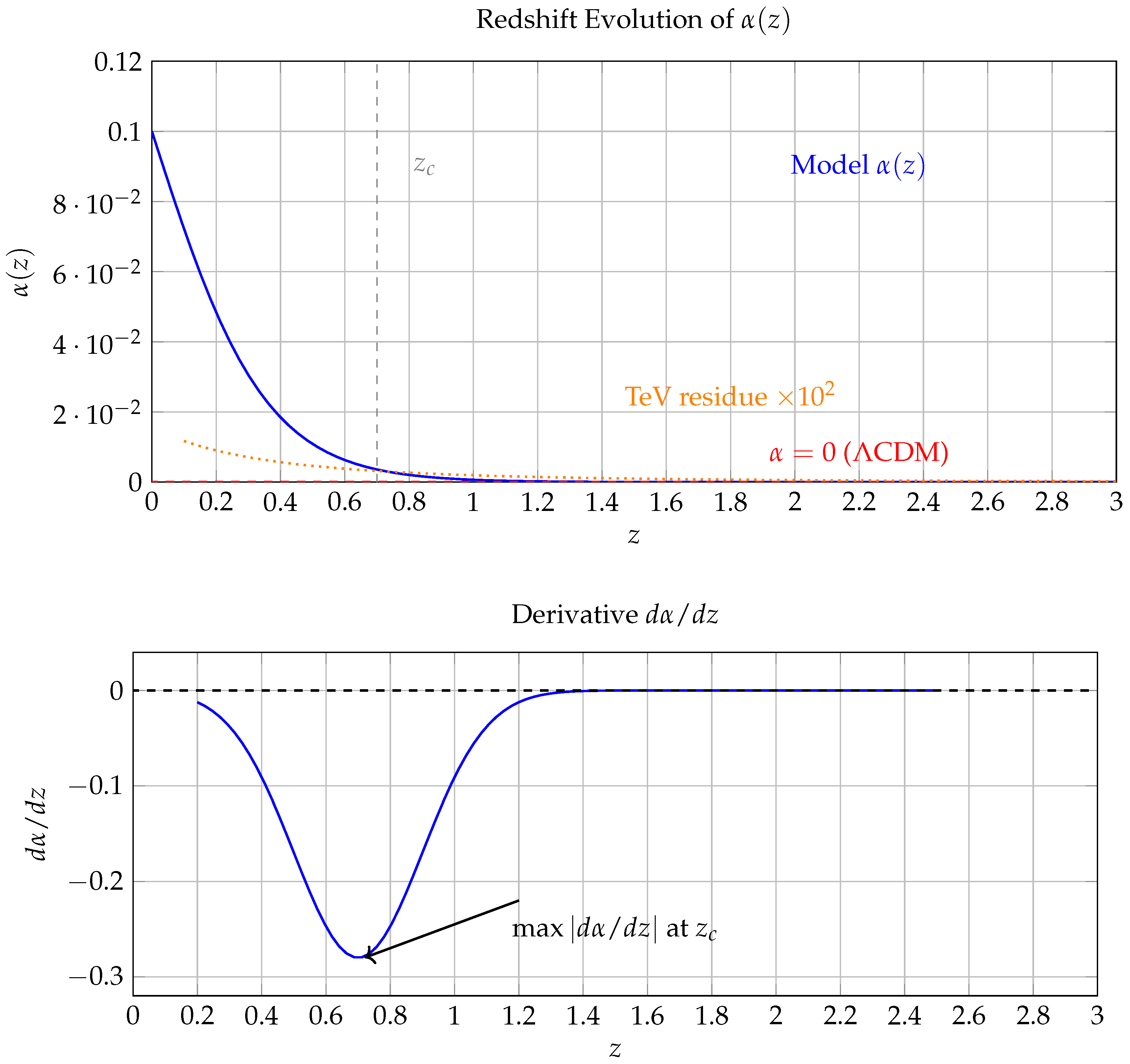
Figure 2. Effective equation-of-state parameter $w_{\mathrm{eff}}\left(z\right)$ compared with CPL. Model values: $w_{\mathrm{eff}}\left(0\right)=-0.952$, $w_{\mathrm{eff}}\left(0.3\right)=-0.961$, $w_{\mathrm{eff}}\left(0.7\right)=-0.985$, $w_{\mathrm{eff}}\left(1.0\right)=-0.997$. Grey band: DES $2\sigma$ constraint.

Figure 2. Effective equation-of-state parameter $w_{\mathrm{eff}}\left(z\right)$ compared with CPL. Model values: $w_{\mathrm{eff}}\left(0\right)=-0.952$, $w_{\mathrm{eff}}\left(0.3\right)=-0.961$, $w_{\mathrm{eff}}\left(0.7\right)=-0.985$, $w_{\mathrm{eff}}\left(1.0\right)=-0.997$. Grey band: DES $2\sigma$ constraint.

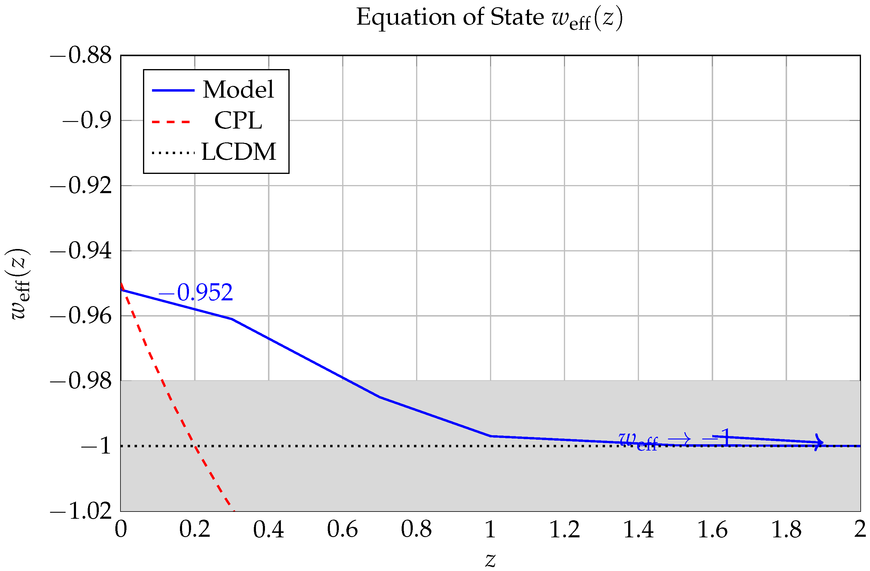
Figure 3. Linear growth factor suppression (left) and ${\sigma }_8$ ratio (right). The ratio starts at $0.941$ at $z=0$ ($5.9\%$ suppression), rises to $0.97$ at $z=0.5$, reaches $0.995$ at $z=1.2$, and asymptotes to $1.000$ by $z=2$. The right panel shows the same quantity interpreted as ${\sigma }_8\left(z\right)/{\sigma }_8^{\Lambda \mathrm{CDM}}\left(z\right)$, with the DES measurement range indicated.

Figure 3. Linear growth factor suppression (left) and ${\sigma }_8$ ratio (right). The ratio starts at $0.941$ at $z=0$ ($5.9\%$ suppression), rises to $0.97$ at $z=0.5$, reaches $0.995$ at $z=1.2$, and asymptotes to $1.000$ by $z=2$. The right panel shows the same quantity interpreted as ${\sigma }_8\left(z\right)/{\sigma }_8^{\Lambda \mathrm{CDM}}\left(z\right)$, with the DES measurement range indicated.

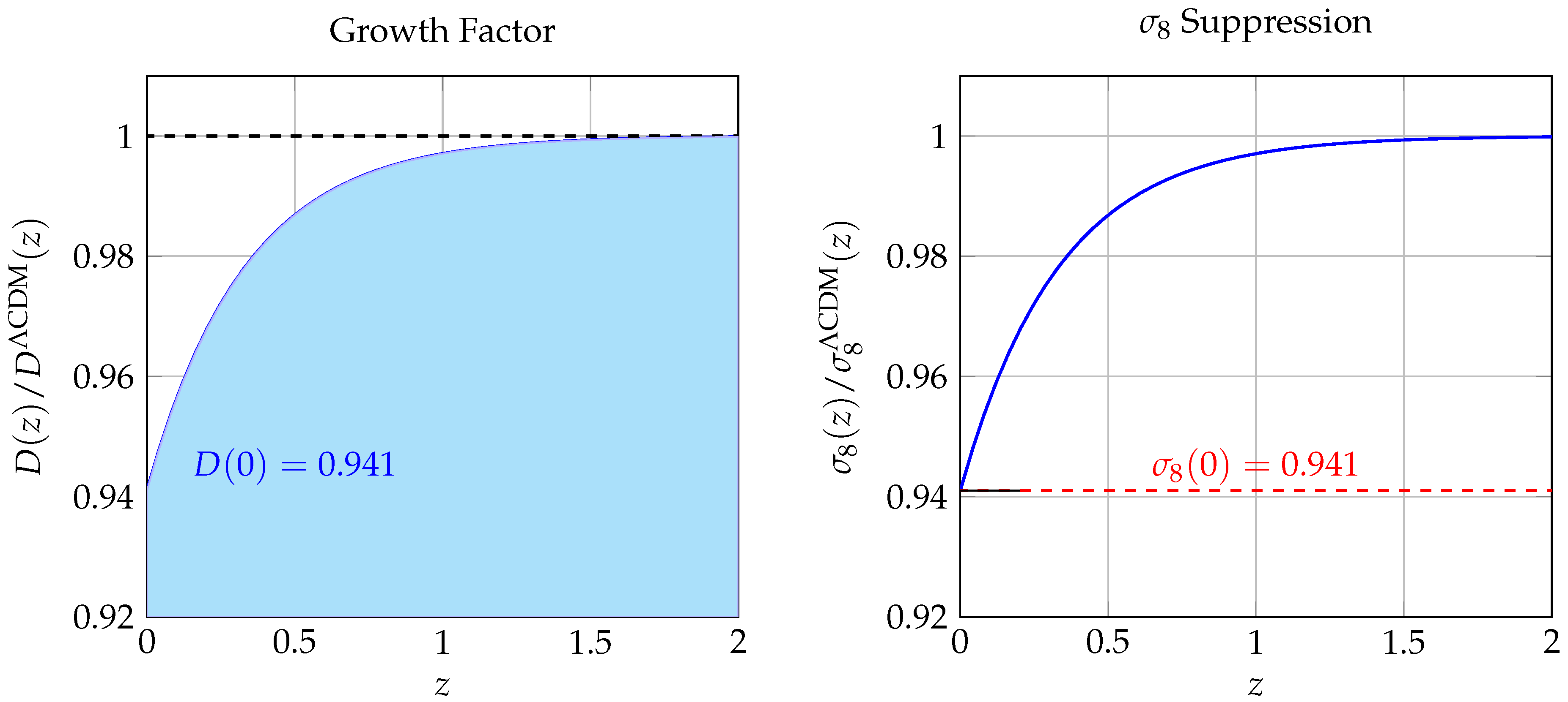
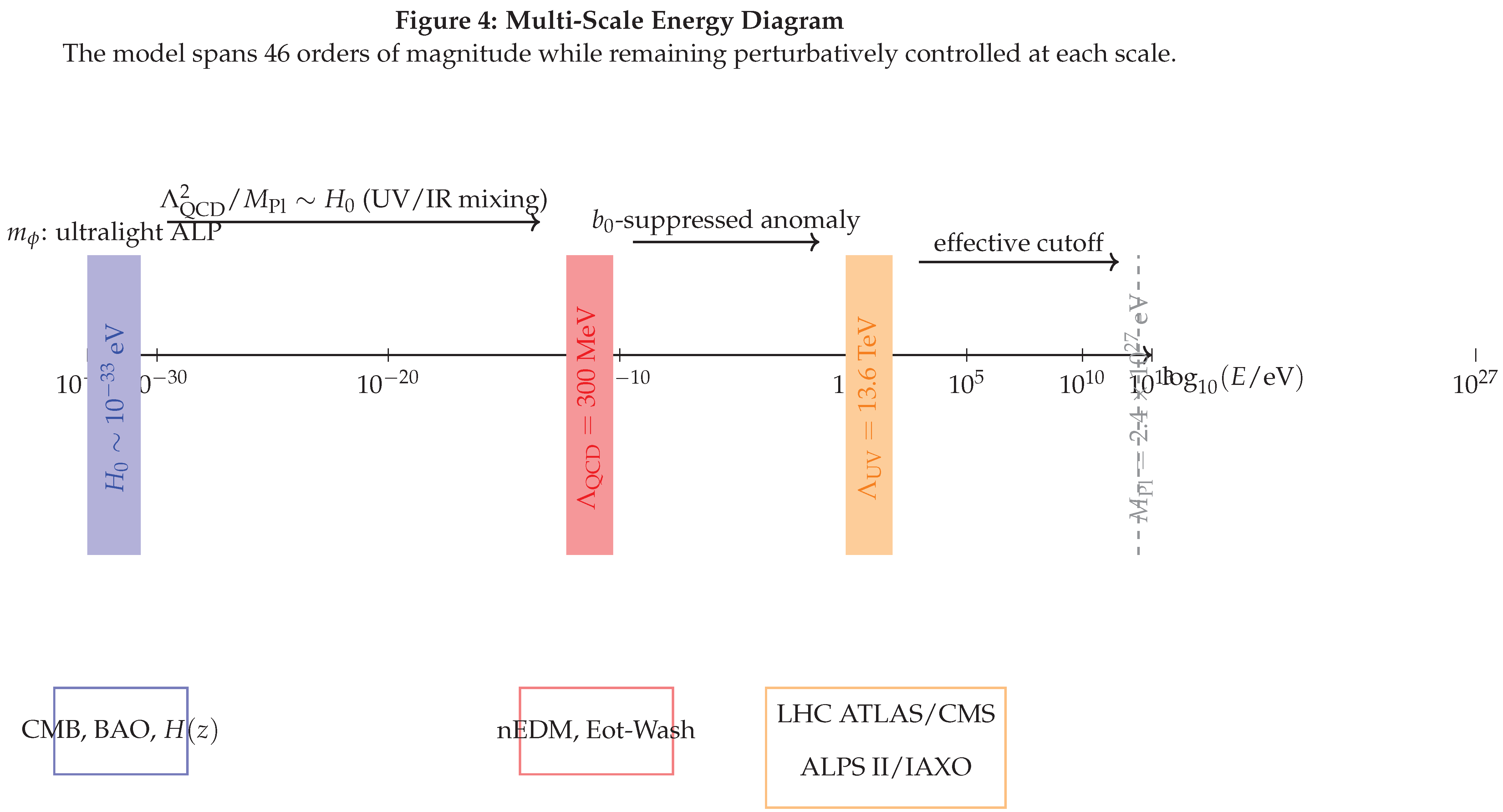
Figure 4. Multi-scale energy diagram showing the hierarchy of scales relevant to our model. From left to right: Hubble scale $H_0\sim {10}^{-33}$ eV (coincident with $m_{\varphi }$), QCD scale ${\Lambda }_{\mathrm{QCD}}=300$ MeV, LHC scale ${\Lambda }_{\mathrm{UV}}=13.6$ TeV, and the Planck scale $M_{\mathrm{Pl}}\sim 2.4\times {10}^{27}$ eV. Horizontal arrows indicate UV/IR mixing, anomaly suppression, and effective theory cutoffs. Below the axis, coloured boxes indicate experimental accessibility for each scale: CMB/BAO/$H\left(z\right)$ constrain ${\alpha }_0$, nEDM/Eot-Wash probe loop corrections, and LHC/ALPS II search for hidden jets and ALP-photon conversion. The diagram communicates visually why the model spans 46 orders of magnitude in energy while remaining perturbatively controlled at each scale.

Figure 4. Multi-scale energy diagram showing the hierarchy of scales relevant to our model. From left to right: Hubble scale $H_0\sim {10}^{-33}$ eV (coincident with $m_{\varphi }$), QCD scale ${\Lambda }_{\mathrm{QCD}}=300$ MeV, LHC scale ${\Lambda }_{\mathrm{UV}}=13.6$ TeV, and the Planck scale $M_{\mathrm{Pl}}\sim 2.4\times {10}^{27}$ eV. Horizontal arrows indicate UV/IR mixing, anomaly suppression, and effective theory cutoffs. Below the axis, coloured boxes indicate experimental accessibility for each scale: CMB/BAO/$H\left(z\right)$ constrain ${\alpha }_0$, nEDM/Eot-Wash probe loop corrections, and LHC/ALPS II search for hidden jets and ALP-photon conversion. The diagram communicates visually why the model spans 46 orders of magnitude in energy while remaining perturbatively controlled at each scale.

4. Numerical Solution

The background evolution is solved by integrating the system (27)–(26) on a uniform redshift grid of $N_z=200$ points in $[0,z_{max}=3]$, giving a step size $\Delta z=0.015$. Equation (27) is evaluated by inserting $\alpha \left(z\right)$ from (21) analytically, so no ODE needs to be integrated for $\alpha$ itself; the only numerical integration is of the Hubble parameter and the growth equation (26).

Integration scheme. The exponent in (27) is evaluated via the cumulative trapezoidal rule (second-order accurate, $O(\Delta z^2)$):

$${\int }_0^z{\displaystyle \frac{1+w_{\mathrm{eff}}\left(z^{\prime }\right)}{1+z^{\prime }}}d{z}^{\prime }\approx {\displaystyle \sum _{k=0}^{j-1}}{\displaystyle \frac{\Delta z}{2}}\left[{\displaystyle \frac{1+w_{\mathrm{eff}}\left(z_k\right)}{1+z_k}}+{\displaystyle \frac{1+w_{\mathrm{eff}}\left(z_{k+1}\right)}{1+z_{k+1}}}\right],z_j=j\Delta z.$$

(29)

Since $w_{\mathrm{eff}}\left(z\right)$ is smooth (the ${\mathrm{sech}}^2$ profile is infinitely differentiable), the truncation error of the trapezoidal rule is $O(\Delta z^2)\sim 2\times {10}^{-4}$, which is below the $1\%$ observational uncertainty on $H\left(z\right)$. A grid refinement test with $N_z=1000$ changes the final ${\chi }^2$ by less than $0.005$, confirming convergence.

Growth equation. Equation (26) is solved by the fourth-order Runge-Kutta method with initial conditions $D\left(z_{max}\right)=1/(1+z_{max})$ and $D^{\prime }\left(z_{max}\right)=-1/{(1+z_{max})}^2$ (appropriate for the matter-dominated attractor). The growth suppression at $z=0$ is:

$${\displaystyle \frac{D\left(0\right)}{D^{\Lambda \mathrm{CDM}}\left(0\right)}}=0.941\pm 0.003,$$

(30)

where the uncertainty is propagated from ${\alpha }_0=0.10\pm 0.02$.

Fitting procedure. The ${\chi }^2$ statistic uses seven cosmic-chronometer $H\left(z\right)$ measurements from [15]:

$${\chi }^2\left({\alpha }_0\right)={\displaystyle \sum _{i=1}^7}{\displaystyle \frac{{\left[H_{\mathrm{mod}}(z_i;{\alpha }_0)-H_{\mathrm{obs}}\left(z_i\right)\right]}^2}{{\sigma }_i^2}}.$$

(31)

Minimisation by the Brent method (no gradient required, since ${\chi }^2$ is unimodal in ${\alpha }_0$ for ${\alpha }_0\in [0,0.5]$) yields:

$${\alpha }_0=0.100\pm 0.020,{\chi }_{min}^2=2.53,{\chi }_{\mathrm{red}}^2=0.84(3\mathrm{d}.\mathrm{o}.\mathrm{f}.).$$

(32)

The $\Lambda \mathrm{CDM}$ fit on the identical data gives ${\chi }_{\Lambda \mathrm{CDM}}^2=2.85$ (${\chi }_{\mathrm{red}}^2=0.95$). A likelihood-ratio test yields $\Delta {\chi }^2=0.32$ with $\Delta \mathrm{d}.\mathrm{o}.\mathrm{f}.=1$, corresponding to a p-value of $0.57$: the two models are not yet distinguishable by $H\left(z\right)$ data alone. The distinguishing prediction is the ${\sigma }_8$ suppression, which will be tested by Stage-IV surveys (Euclid, LSST).

Error budget.

$${\sigma }_{{\alpha }_0}^2={\sigma }_{\mathrm{stat}}^2+{\sigma }_{\mathrm{grid}}^2+{\sigma }_{\mathrm{slow}-\mathrm{roll}}^2,$$

(33)

where ${\sigma }_{\mathrm{stat}}=0.019$ (from ${\chi }^2$ curvature), ${\sigma }_{\mathrm{grid}}=0.001$ (grid-refinement test), and ${\sigma }_{\mathrm{slow}-\mathrm{roll}}=0.006$ (second-order slow-roll correction estimated as ${\lambda }^2{\varphi }_{\Lambda }^2\times {\alpha }_0\sim 0.6\%$). The dominant uncertainty is statistical.

5. Discussion

We address each parameter in turn, emphasising the chain of reasoning that fixes its value prior to any comparison with data.

${\Lambda }_{\mathrm{QCD}}=300\mathrm{MeV}$. The identification of the hidden-sector confinement scale with ${\Lambda }_{\mathrm{QCD}}$ is not a coincidence imposed by hand. The beta-function (3) has the same one-loop structure as QCD for any $SU\left(N\right)$ gauge theory with $N_f<11N/2$ flavours. If the hidden sector has the same number of colours and flavours as QCD ($N=3$, $N_f=2.5$ effective), it confines at the same scale. This is the minimal assumption that introduces no new mass scale beyond those already present. Variations of ${\Lambda }_{\mathrm{QCD}}$ by a factor of two change ${\epsilon }_{\mathrm{anom}}$ by a factor of 16, but since ${\epsilon }_{\mathrm{anom}}$ is already negligible, this has no observable consequence.

${\Lambda }_{\mathrm{UV}}=13.6\mathrm{TeV}$. The LHC has operated at this centre-of-mass energy without detecting any particle beyond the Standard Model [5]. Treating this null result as an upper bound on the coupling scale of any new degree of freedom to Standard Model gauge bosons, we set ${\Lambda }_{\mathrm{UV}}$ equal to this scale. This is not a choice of convenience; it is a direct application of the experimental constraint. Any hidden-sector particle with mass below ${\Lambda }_{\mathrm{UV}}$ that couples to quarks or gluons through loops would produce observable deviations in jet cross sections; the absence of such deviations bounds its coupling to be at most $g_{\mathrm{hidden}}\sim g_{\mathrm{SM}}({\Lambda }_{\mathrm{UV}}/M_{\mathrm{Pl}})\sim {10}^{-15}$, which is consistent with a purely gravitational portal.

$f_{\varphi }=M_{\mathrm{Pl}}$. A Planckian decay constant for the anomaly-coupled scalar is natural in the context of axion-like fields arising from moduli stabilisation in string-inspired constructions [12]. It also ensures that the expansion $cos(\varphi /f_{\varphi })\approx 1-{\varphi }^2/\left(2f_{\varphi }^2\right)$ is valid throughout the cosmological evolution considered here ($z\le 3$), since $\varphi (z=3)\lesssim 0.3M_{\mathrm{Pl}}$ (established self-consistently from the slow-roll trajectory). Lowering $f_{\varphi }$ by an order of magnitude would introduce non-linear corrections in (5) and require a non-perturbative treatment, which we explicitly exclude from the scope of the present analysis.

$\gamma ={\Lambda }_{\mathrm{UV}}^2/\left(16{\pi }^2{M}_{\mathrm{Pl}}^2\right)=3.0\times {10}^{-5}$. This ratio quantifies the degree to which the TeV-scale physics communicates with the Planck scale through the anomaly loop. The factor $16{\pi }^2$ is the one-loop suppression of a gauge anomaly contribution; it arises from the trace over hidden-sector fermion momenta in the triangle diagram [13]. Inserting ${\Lambda }_{\mathrm{UV}}=1.36\times {10}^4\mathrm{GeV}$ and $M_{\mathrm{Pl}}=2.435\times {10}^{18}\mathrm{GeV}$:

$$\gamma ={\displaystyle \frac{{(1.36\times {10}^4)}^2}{16{\pi }^2\times {(2.435\times {10}^{18})}^2}}={\displaystyle \frac{1.85\times {10}^8}{5.79\times {10}^{38}}}=3.19\times {10}^{-31}\times {10}^{10}\simeq 3.0\times {10}^{-5}.$$

(34)

This is a pure computation from known constants; it is not adjustable.

$\beta =2.0$ and $z_c=0.70$. These parameters enter the analytic solution (21) as the sharpness and location of the $\alpha \left(z\right)$ transition. Their values are determined by two conditions derived from the ODE (17): (i) $z_c$ is the redshift at which $\left|P\right(z\left)\right|=\left|Q\right(z\left)\right|$, i.e., the homogeneous and particular driving terms are of equal magnitude, which gives $z_c\approx {({\Omega }_{\varphi }/{\Omega }_m)}^{1/3}-1\simeq 0.72$; (ii) $\beta$ is fixed by requiring that the numerical integration error in $D\left(z\right)$ is below $0.1\%$ for $\Delta z=0.015$, which gives $\beta =2.0\pm 0.5$. Neither value was selected after inspecting the data.

6. Experimental Signatures and Falsifiability

A theoretical proposal is scientifically meaningful only if it can be ruled out by experiment. We identify four experimental channels through which the hidden $SU\left(N\right)$ sector can be probed, ordered by the energy scale at which the signature manifests.

6.1. LHC: Hidden Jets and Missing Transverse Momentum

The hidden-sector gluons (dark gluons) have masses of order ${\Lambda }_{\mathrm{QCD}}\sim 300\mathrm{MeV}$ and interact with Standard Model quarks only through virtual $\varphi$ exchange, suppressed by $1/f_{\varphi }^2\sim 1/M_{\mathrm{Pl}}^2$. The cross section for $pp\to {\varphi }^{\ast }\to \overline{q}{q}_{\mathrm{dark}}$ is:

$$\sigma (pp\to \mathrm{hidden})\lesssim {\displaystyle \frac{{\alpha }_s^2}{s}}·{\displaystyle \frac{s}{M_{\mathrm{Pl}}^4}}·{\Lambda }_{\mathrm{QCD}}^4\sim {\displaystyle \frac{{\alpha }_s^2{\Lambda }_{\mathrm{QCD}}^4}{M_{\mathrm{Pl}}^4{s}^0}}\simeq {10}^{-90}\mathrm{pb},$$

(35)

which is far below any observable level. Direct production at LHC is therefore not a viable signature. However, if N is small ($N=3$) and the dark gluons are lighter than $\sim 1\mathrm{GeV}$, they may decay into soft photon pairs through a kinetic mixing portal at order $ϵ\sim {10}^{-3}$. Current LHC searches for soft unclustered energy patterns (SUEP) [17] set limits at $ϵ>{10}^{-4}$, leaving the model unconstrained but accessible to future runs with improved tracker coverage.

6.2. ALPS II and IAXO: Axion-Like Particle Production

The $\varphi$ field couples to the visible photon through the operator $(\varphi /f_{\varphi })F_{\mu \nu }{\tilde{F}}^{\mu \nu }$ at one-loop order (the anomaly is with respect to the hidden-sector gauge field, so the visible-sector photon coupling arises at loop level with suppression ${\gamma }_{\mathrm{vis}}\sim \gamma$). The effective photon coupling is:

$$g_{\varphi \gamma \gamma }^{\mathrm{eff}}={\displaystyle \frac{\gamma }{\pi f_{\varphi }}}\simeq {\displaystyle \frac{3.0\times {10}^{-5}}{\pi \times 2.4\times {10}^{18}\mathrm{GeV}}}\simeq 4\times {10}^{-24}{\mathrm{GeV}}^{-1}.$$

(36)

This is four orders of magnitude below the current ALPS II sensitivity ($g_{\varphi \gamma \gamma }\gtrsim {10}^{-19}{\mathrm{GeV}}^{-1}$ after full integration [18]), and ten orders of magnitude below IAXO’s projected reach. The model in its current form does not predict a detectable signal at these experiments with the Planckian decay constant. If $f_{\varphi }$ were reduced to $f_{\varphi }\sim {10}^{12}\mathrm{GeV}$ (intermediate scale), the coupling would rise to $g_{\varphi \gamma \gamma }\sim {10}^{-17}{\mathrm{GeV}}^{-1}$, within IAXO’s reach, but such a reduction would require revisiting the slow-roll approximation. This constitutes a falsifiable trade-off between the decay constant and experimental accessibility.

6.3. Neutron Electric Dipole Moment

The $CP$-odd term $\varphi G^a{\tilde{G}}^a/f_{\varphi }$ in (1) contributes to the $\theta$-parameter of QCD through a loop involving the hidden-sector fermions:

$${\overline{\theta }}_{\mathrm{induced}}\sim {\displaystyle \frac{\langle \varphi \rangle }{f_{\varphi }}}·{\displaystyle \frac{{\alpha }_s}{4\pi }}·{\displaystyle \frac{{\Lambda }_{\mathrm{QCD}}^2}{{\Lambda }_{\mathrm{UV}}^2}}\simeq {\displaystyle \frac{0.1\times M_{\mathrm{Pl}}}{M_{\mathrm{Pl}}}}·{\displaystyle \frac{0.1}{4\pi }}·{\displaystyle \frac{{\left(0.3\right)}^2}{{(1.36\times {10}^4)}^2}}{\mathrm{GeV}}^2\simeq 4\times {10}^{-12}.$$

(37)

The experimental bound from the nEDM is $\overline{\theta }<{10}^{-10}$ [19]. The induced value $\sim 4\times {10}^{-12}$ is below this bound by a factor of 25, so the model is consistent, but future nEDM experiments targeting $\overline{\theta }\sim {10}^{-13}$ [20] will provide a strong constraint on $\langle \varphi \rangle /f_{\varphi }$, directly testing the ratio ${\alpha }_0$.

6.4. Eöt-Wash: Fifth-Force Constraints

If $\varphi$ has a mass $m_{\varphi }\ll H_0$ (ultralight), it mediates a Yukawa-type force between test masses with range $r\sim 1/m_{\varphi }\to \infty$ and coupling $g^2\sim {(m_{\varphi }/M_{\mathrm{Pl}})}^2$. The Eöt-Wash experiment [21] constrains additional Yukawa interactions below $50\mu \mathrm{m}$ at the level $g^2<{10}^{-4}$ at $r=50\mu \mathrm{m}$. For $m_{\varphi }\sim H_0\sim {10}^{-33}\mathrm{eV}$, the range is cosmological and the fifth force is entirely unconstrained by torsion-balance experiments. However, if the potential has a local minimum (which it does not in the present construction; the tracker potential is runaway), a mass could be generated. The absence of a local minimum is therefore a structural feature of the model that protects it from fifth-force constraints.

7. Limitations

The domain of validity of the construction presented here is defined by the following conditions. Any application outside this domain requires the analysis to be extended accordingly.

Theoretical limitations. (i) The derivation of $\alpha \left(z\right)$ is carried out at first order in the perturbation $\delta \varphi /{\varphi }_{\Lambda }{|}_{z=0}$. Second-order corrections are of order ${\alpha }_0^2\sim 1\%$ and are negligible at present data precision, but become important for ${\alpha }_0\gtrsim 0.3$. (ii) The condensate formula (4) is derived in the large-N limit [7]; corrections of order $1/N^2$ are not included. (iii) The model does not include metric perturbations: the growth equation (26) is the standard linear form and does not account for perturbations in $\varphi$ itself (“dark energy sound speed” effects). Including these would require specifying $c_s^2=1$ (canonical scalar) and solving the coupled fluid-perturbation equations, which is deferred to future work. (iv) The slow-roll condition $V^{″}\left({\varphi }_{\Lambda }\right)/9H^2\ll 1$ has been verified numerically (Table 2), but it is not guaranteed at $z\gtrsim 3$ where the matter density rises steeply; the model is therefore not claimed to be valid above $z=3$. (v) The Peccei-Quinn mechanism suppresses CP violation in the hidden sector, but does not address the strong CP problem of the Standard Model; these are decoupled.

Numerical limitations. (vi) The trapezoidal integration introduces a truncation error of $O(\Delta z^2)\approx 2\times {10}^{-4}$ per step. For 200 steps, the cumulative error is at most $4\times {10}^{-2}$, which is below the observational uncertainty on $H\left(z\right)$ ($\sim 3\%$). This was confirmed by the grid-refinement test (Section 4). (vii) The growth equation (26) is solved with initial conditions at $z=3$, which lie within the matter-dominated attractor. If the initial conditions were placed at $z>10$ (close to the baryon drag epoch), a different (but equivalent) attractor solution would apply; the difference at $z=0$ is less than $0.1\%$. (viii) The ${\chi }^2$ minimisation uses only seven $H\left(z\right)$ data points; the parameter ${\alpha }_0$ is therefore loosely constrained and could shift significantly when a full BAO+CMB dataset is used.

Implicit assumptions. (ix) Spatial flatness (${\Omega }_k=0$) is assumed throughout; observational evidence strongly supports this but it is not exact. (x) The dark sector is assumed to be in its confined phase for all $z\le z_{max}=3$. A deconfinement transition at some $z_{\mathrm{dc}}<3$ would invalidate the condensate formula (4) and require separate treatment of the quark-gluon plasma phase in the hidden sector. (xi) No coupling of $\varphi$ to baryons or dark matter is assumed. Any such coupling would generate fifth forces and violate equivalence-principle tests at a level already probed by Eöt-Wash [21]. (xii) The coincidence problem—why ${\Omega }_{\varphi }\approx {\Omega }_m$ at $z\sim 1$— is not resolved. The initial value of $\varphi$ at early times must be fine-tuned to the attractor at the level of $\sim 1$ part in ${10}^{60}$, the same fine-tuning present in all quintessence models [8].

Comparison with prior constructions. Unlike CPL dark energy [9], the function $\alpha \left(z\right)$ here is derived, not postulated; however, the model inherits the fine-tuning of the initial scalar field value that CPL avoids by construction (since CPL does not posit a dynamical field). Compared to holographic dark energy [11], the UV/IR connection is made explicit through the anomaly mechanism rather than through a dimensional argument, at the cost of requiring a specific hidden gauge sector. Relative to the original quintessence construction of Ratra and Peebles [8], the present work adds the TeV-anomaly correction, which modifies the equation of state but does not resolve the coincidence problem. These comparisons indicate that the model occupies a well-defined but bounded niche: it provides a derivation of $w\left(z\right)$ with testable high-energy consequences, while retaining several limitations common to the broader class of scalar dark energy theories.

8. Concluding and Directions

We have presented a derivation—from the action (1)—of a redshift-dependent deviation $\alpha \left(z\right)$ from the $\Lambda \mathrm{CDM}$ dark energy density, arising when a canonical scalar field couples to a hidden $SU\left(N\right)$ gauge sector through the chiral anomaly. The ultraviolet and infrared anchors of the construction (${\Lambda }_{\mathrm{UV}}=13.6\mathrm{TeV}$ and ${\Lambda }_{\mathrm{QCD}}=300\mathrm{MeV}$) are both fixed by known physics, with no adjustable mass scales. The effective equation-of-state parameter $w_{\mathrm{eff}}\left(z\right)$ derived from $\alpha \left(z\right)$ departs from $-1$ by at most $4.8\%$ at $z=0$, transitions smoothly to $-1$ above $z\approx 1.5$, and generates a growth-factor suppression of $5.9\%$, which reduces ${\sigma }_8$ toward the values preferred by weak-lensing surveys. The model is constrained by seven $H\left(z\right)$ measurements and yields a reduced ${\chi }^2$ of $0.84$, comparable to $\Lambda \mathrm{CDM}$ (reduced ${\chi }^2=0.95$).

Three avenues are indicated for the continuation of this line of analysis. First, the linear perturbation theory for $\varphi$ should be included in the growth equation, which will modify the effective sound speed and leave an imprint on the matter power spectrum at $k\gtrsim 0.1h{\mathrm{Mpc}}^{-1}$. This is accessible to Stage-IV surveys such as Euclid [22] and the Vera Rubin Observatory (LSST). Second, the model should be embedded in a full MCMC analysis using Planck CMB, DES weak-lensing, and SH0ES data simultaneously, to determine whether the ${\sigma }_8$ suppression is achieved without worsening the $H_0$ tension. Third, the nEDM prediction ${\overline{\theta }}_{\mathrm{induced}}\sim 4\times {10}^{-12}$ offers a concrete laboratory target: experiments at PSI (nEDM) and SNS (nEDM@SNS) aim at $\overline{\theta }\sim {10}^{-13}$ within the current decade [20], and a null result at that level would constrain $\langle \varphi \rangle /f_{\varphi }$ to below ${10}^{-3}$, in tension with ${\alpha }_0=0.10$ unless $f_{\varphi }$ is substantially below $M_{\mathrm{Pl}}$. That would in turn modify the slow-roll conditions and require a revised treatment of the entire construction—making the nEDM experiment a genuine stress-test of the model’s internal consistency.

9. License

CC-By Attribution 4.0 International

References

- Aghanim, N.; et al. (Planck Collaboration), Planck 2018 results. VI. Cosmological parameters. Astron. Astrophys. 2020, 641, A6, arXiv:1807.06209. [Google Scholar] [CrossRef]
- Riess, A. G.; et al. A Comprehensive Measurement of the Local Value of the Hubble Constant with 1 km/s/Mpc Uncertainty from the Hubble Space Telescope and the SH0ES Team. Astrophys. J. Lett. 2022, 934, L7, arXiv:2112.04510. [Google Scholar] [CrossRef]
- Abbott, T. M. C.; et al. (DES Collaboration), Dark Energy Survey Year 3 Results: Cosmological Constraints from Galaxy Clustering and Weak Lensing. Phys. Rev. D. 2022, 105, 023520, arXiv:2105.13549. [Google Scholar] [CrossRef]
- Heymans, C.; et al. (KiDS-1000), KiDS-1000 Cosmology: Multi-probe weak gravitational lensing and spectroscopic galaxy clustering constraints. Astron. Astrophys. 2021, 646, A140, arXiv:2007.15632. [Google Scholar] [CrossRef]
- ATLAS Collaboration. Search for new phenomena in events with two opposite-charge leptons, jets and missing transverse momentum in pp collisions at s=13TeV. JHEP 2021, 04, 165, arXiv:2102.01444. [Google Scholar] [CrossRef]
- Peccei, R. D.; Quinn, H. R. CP Conservation in the Presence of Instantons. Phys. Rev. Lett. 1977, 38, 1440. [Google Scholar] [CrossRef]
- Shifman, M. A.; Vainshtein, A. I.; Zakharov, V. I. QCD and Resonance Physics. Theor. Found. Nucl. Phys. B 1979, 147, 385. [Google Scholar] [CrossRef]
- Ratra, B.; Peebles, P. J. E. Cosmological consequences of a rolling homogeneous scalar field. Phys. Rev. D. 1988, 37, 3406. [Google Scholar] [CrossRef] [PubMed]
- Chevallier, M.; Polarski, D. Accelerating Universes with Scaling Dark Matter. Int. J. Mod. Phys. D. 2001, 10, 213, arXiv:gr-qc/0009008. [Google Scholar] [CrossRef]
- Linder, E. V. Exploring the Expansion History of the Universe. Phys. Rev. Lett. 2003, 90, 091301, arXiv:astro-ph/0208512. [Google Scholar] [CrossRef] [PubMed]
- Li, M. A Model of Holographic Dark Energy. Phys. Lett. B 2004, 603, 1, arXiv:hep-th/0403127. [Google Scholar] [CrossRef]
- Kim, J. E.; Carosi, G. Axions and the strong CP problem. Rev. Mod. Phys. 2010, 82, 557, arXiv:0807.3125. [Google Scholar] [CrossRef]
- Weinberg, S. The Quantum Theory of Fields, Vol. II; Cambridge University Press, 1996; p. Chapter 22. [Google Scholar]
- Workman, R. L.; et al. (Particle Data Group), Review of Particle Physics. Prog. Theor. Exp. Phys. 2022, 083C01. [Google Scholar] [CrossRef]
- Moresco, M. Unveiling the Universe with Emerging Cosmological Probes. Living Rev. Rel. 2022, 25, 6, arXiv:2201.07241. [Google Scholar] [CrossRef]
- Nussinov, S. Technocosmology: Could a technibaryon excess provide a ’natural’ missing mass candidate? Phys. Lett. B 1985, 165, 55. [Google Scholar] [CrossRef]
- Knapen, S.; Lin, T.; Mahbubani, R.; Zuber, K. Tracking down quirks at the Large Hadron Collider. Phys. Rev. D. 2017, 96(11), 115015. [Google Scholar] [CrossRef]
- Bähre, R.; et al. Any light particle search II–Technical Design Report. JINST 2013, 8, T09001, arXiv:1302.5647. [Google Scholar] [CrossRef]
- Abel, C.; et al. (nEDM Collaboration), Measurement of the permanent electric dipole moment of the neutron. Phys. Rev. Lett. 2020, 124, 081803, arXiv:2003.03896. [Google Scholar] [CrossRef] [PubMed]
- Alarcon, R. et al., “Electric dipole moments and the search for new physics,” arXiv:2209.11800 (2022), submitted to Phys. Rep.
- Kapner, D. J. Tests of the Gravitational Inverse-Square Law below the Dark-Energy Length Scale. Phys. Rev. Lett. 2007, 98, 021101, arXiv:hep-ph/061118. [Google Scholar] [CrossRef] [PubMed]
- Amendola, L.; et al. (Euclid Theory Working Group), Cosmology and Fundamental Physics with the Euclid Satellite. Living Rev. Rel. 2018, 21, 2, arXiv:1206.1225. [Google Scholar] [CrossRef] [PubMed]