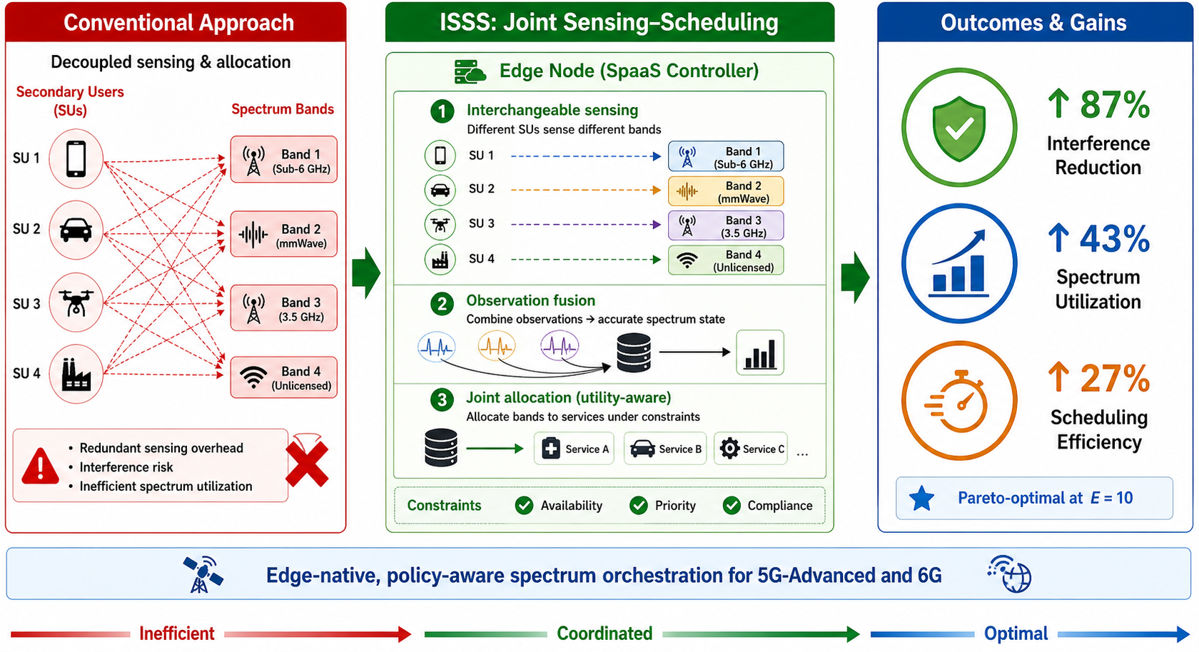
Submitted:
02 May 2026
Posted:
05 May 2026
You are already at the latest version
Abstract

Keywords:
1. Introduction
1.1. Limitations of Existing Approaches
1.2. The ISSS Approach
1.3. Contributions of This Work
1.4. Paper Organization
2. Related Work
3. System Model and Problem Formulation
3.1. Edge-Based SpaaS Control Model
3.2. Spectrum Availability as a Schedulable State
3.3. Service-Centric Spectrum Allocation
3.4. Joint Sensing–Scheduling Objective
3.5. Constraints and Governance Awareness
- Availability constraint (feasibility):
-
Exclusivity constraint (contention control):Each band can be assigned to at most one service at a given time interval, preventing conflicting simultaneous use.
-
Service priority constraint (policy enforcement):Allocation decisions must respect service priorities , reflecting SLA requirements, criticality, or regulatory preference.
-
Regulatory compliance constraint (governance adherence):
3.6. Interchangeability Principle
- temporal freshness of sensing information, and
- spatial diversity of observations.
3.7. Practical Complexity and Edge Feasibility
3.8. Architectural Logic Underpinning ISSS Performance
| Algorithm 1. ISSS Edge Controller — Per Control Interval. |
| Input: B — set of spectrum bands U — set of services with weights w_u c_b(t) — sensing cost per band at time t λ — sensing cost weight {obs_{n,b}} — observations from E sensing nodes Output: x_{u,b}(t), s_b(t), O_ISSS Step 1 — Interchangeable sensing assignment Partition B across E nodes via round-robin interchangeable schedule For each band b ∈ B: Assign b to one dedicated node; set s_b(t) = 1 O_ISSS ← |B| · log₂(E + 1) Step 2 — Observation fusion For each band b ∈ B: If mean_n{obs_{n,b}} ≥ 0.5 then â_b(t) ← 1 (band estimated idle) Else â_b(t) ← 0 (band estimated busy) Step 3 — Joint allocation For each service u ∈ U, ranked by descending w_u: For each band b ∈ B, ranked by descending score(u,b): score(u,b) ← w_u · â_b(t) − λ · c_b(t) If C1: â_b(t) = 1 (availability) And C2: Σ_u x_{u,b}(t) = 0 (exclusivity) And C3: w_u ≥ w_{u’} for all previously allocated u’ (priority) And C4: access compliant with incumbent rules (compliance) Then x_{u,b}(t) ← 1; break to next service Else x_{u,b}(t) ← 0; try next band Step 4 — Return x_{u,b}(t), s_b(t), O_ISSS |
4. Performance Evaluation and Quantified ISSS Contribution
4.1. Evaluation Framework and System Configuration
4.2. Primary User Channel Model and Detection Parameters
| Regime | Interpretation | |
| Low PU activity | 0.15 | Predominantly idle; maximum access opportunity |
| Medium PU activity | 0.40 | Mixed occupancy; representative operational scenario |
| High PU activity | 0.70 | Predominantly occupied; stringent incumbent protection required |
4.3. Performance Metrics
4.3.1. Interference Reduction Gain
4.3.2. Spectrum Utilization Gain
4.3.3. Scheduling Efficiency Gain
4.4. Simulation Procedure
| Algorithm 2: Monte Carlo Evaluation Procedure — Per Control Interval |
| Input: E (edge nodes), P_busy, P_d,s, P_f,s, λ, |B|, w_u Output: G_I(E), G_U(E), G_S(E) Initialise: I_single=0, I_ISSS=0, I_coop=0 U_single=0, U_ISSS=0, U_coop=0 O_single=0, O_ISSS=0, O_coop=0 For t = 1 to N_MC: // Generate true spectrum availability (Sec. 3.2) For each band b ∈ B: a_b(t) = 1 if U[0,1] > P_busy (idle) = 0 otherwise (busy) // ── Configuration 1: Single-edge baseline ── For each band b ∈ B: If a_b(t) = 1: x_s(b) = 1 if U[0,1] < P_d,s else 0 Else: x_s(b) = 1 if U[0,1] < P_f,s else 0 I_single += Σ_b x_s(b) · (1 − a_b(t)) // false alarms → interference U_single += Σ_b w_u · x_s(b) · a_b(t) // correct access → utility O_single += |B| // ── Configuration 2: Cooperative sensing (E nodes, no scheduling) ─ For each node n = 1 to E: For each band b ∈ B: obs_c(n,b) = sense(a_b(t), P_d,s, P_f,s) // standard Pd/Pf x_c(b) = 1 if mean_n{obs_c(n,b)} ≥ 0.5 else 0 // majority vote I_coop += Σ_b x_c(b) · (1 − a_b(t)) U_coop += Σ_b w_u · x_c(b) · a_b(t) O_coop += E · |B| //Configuration 3: ISSS — executes Algorithm 1 (Sec. 3.4, 3.5, 3.6) // Compute interchangeability-enhanced parameters (Sec. 3.6) factor = 1 − exp(−(E−1) / τ) // saturation model P_d,i = P_d,s + (P_d,max − P_d,s) · factor · (1 − ξ_d · P_busy) P_f,i = P_f,s − (P_f,s − P_f,min) · factor · (1 − ξ_f · P_busy) P_d,i = min(0.99, P_d,i); P_f,i = max(0.01, P_f,i) For each node n = 1 to E: For each band b ∈ B: obs_i(n,b) = sense(a_b(t), P_d,i, P_f,i) // improved sensing // Joint scheduling decision: access if confidence ≥ 0.5 x_i(b) = 1 if mean_n{obs_i(n,b)} ≥ 0.5 else 0 // Joint objective evaluation (Sec. 3.4): // J = Σ_b w_u·x_i(b) − λ · Σ_b c_b(t)·s_b(t) J = U_ISSS_slot − λ · O_ISSS_slot / |B| I_ISSS += Σ_b x_i(b) · (1 − a_b(t)) U_ISSS += Σ_b w_u · x_i(b) · a_b(t) O_ISSS += |B| · log₂(E+1) // sub-linear overhead (Sec. 3.6) End For // Compute gain metrics (Sec. 4.3) G_I(E) = (1 − I_ISSS / I_single) × 100% G_U(E) = ((U_ISSS − U_single) / U_single) × 100% G_S(E) = (1 − O_ISSS / O_coop) × 100% |
4.5. Results and Discussion
4.5.1. Interference Reduction Gain
4.5.2. Pareto Efficiency Frontier: ( vs. )
4.5.3. Multi-Metric Gain Profile
4.6. Consolidated Gain Analysis and Pareto-Optimal Operating Point
5. Conclusions
Author Contributions
Funding
Data Availability Statement
Acknowledgments
Conflicts of Interest
Abbreviations
| ISSS | Interchangeable Spectrum Sensing Scheduling |
| SpaaS | Spectrum-as-a-Service |
| 5G | Fifth Generation |
| 6G | Sixth Generation |
| MEC | Multi-Access Edge Computing |
| CBRS | Citizens Broadband Radio Service |
| LSA | Licensed Shared Access |
| PU | Primary User |
| SLA | Service-Level Agreement |
| URLLC | Ultra-Reliable Low-Latency Communication |
| IoT | Internet of Things |
| RAN | Radio Access Network |
| CR | Cognitive Radio |
References
- Popovski, P.; Trillingsgaard, K.F.; Simeone, O.; Durisi, G. 5G wireless network slicing for eMBB, URLLC, and mMTC: A communication theoretic view. IEEE Access 2018, 6, 55765–55779. [Google Scholar] [CrossRef]
- Abouaomar, A.; Cherkaoui, S.; Mlika, Z.; Kobbane, A. Resource provisioning in edge computing for latency-sensitive applications. IEEE Internet Things J. 2021, 8, 11088–11099. [Google Scholar] [CrossRef]
- Patil, A.; Prasad, R.; Skouby, K.E.; Prasad, N.R. A comprehensive survey on spectrum sharing techniques for 5G/B5G intelligent wireless networks. Comput. Netw. 2024, 224, 109608. [Google Scholar] [CrossRef]
- Bhattarai, S.; Park, J.M.; Gao, B.; Bian, K.; Lehr, W. A survey on Citizens Broadband Radio Service. Electronics 2022, 11, 3891. [Google Scholar] [CrossRef]
- Massaro, M.; Beltrán, F. Untangling the paradox of Licensed Shared Access: Need for regulatory refocus. Telecommun. Policy 2022, 46, 102380. [Google Scholar] [CrossRef]
- Akyildiz, I.F.; Lo, B.F.; Balakrishnan, R. Cooperative spectrum sensing in cognitive radio networks: A survey. Phys. Commun. 2011, 4, 40–62. [Google Scholar] [CrossRef]
- Ghasemi, A.; Sousa, E.S. Spectrum sensing in cognitive radio networks: Requirements, challenges and design trade-offs. IEEE Commun. Mag. 2008, 46, 32–39. [Google Scholar] [CrossRef]
- Federal Communications Commission (FCC). Report and Order and Second Further Notice of Proposed Rulemaking, FCC 15-47; FCC: Washington, DC, USA, 2015. Available online: https://www.fcc.gov/document/fcc-15-47 (accessed on 1 May 2025).
- Ofcom. TV White Spaces: Consultation on White Space Device Requirements; Ofcom: London, UK, 2012; Available online: https://www.ofcom.org.uk/spectrum/spectrum-management/tv-white-spaces (accessed on 1 May 2025).
- Kryszkiewicz, P.; Kliks, A.; Kułacz, Ł.; Bogucka, H.; Koudouridis, G.P.; Dryjański, M. Context-based spectrum sharing in 5G wireless networks based on radio environment maps. Wirel. Commun. Mob. Comput. 2018, 2018, 3217315. [Google Scholar] [CrossRef]
- ETSI. MEC Support for Edge Native Design: An Application Developer Perspective; ETSI: Sophia Antipolis, France, 2023; Available online: https://www.etsi.org/deliver/etsi_wp/55_99/55/01.01.01_60/wp_055e.pdf (accessed on 1 May 2025).
- Taleb, T.; Samdanis, K.; Mada, B.; Flinck, H.; Dutta, S.; Sabella, D. On multi-access edge computing: A survey of the emerging 5G network edge cloud architecture and orchestration. IEEE Commun. Surv. Tutor. 2017, 19, 1657–1681. [Google Scholar] [CrossRef]
- Moubayed, A.; Ahmed, T.; Haque, A.; Shami, A. Machine learning towards enabling Spectrum-as-a-Service dynamic sharing. In Proceedings of the IEEE Canadian Conference on Electrical and Computer Engineering (CCECE), London, ON, Canada, 30 August–2 September 2020. [Google Scholar] [CrossRef]
- ITU-R., S.M. 2405-1: Spectrum Management Principles for Cognitive Radio Systems; ITU: Geneva, Switzerland, 2021; Available online: https://www.itu.int/rec/R-REC-SM.2405/en (accessed on 1 May 2025).
- Salih, S.H.O.; Erman, M.; Mohammed, A. A novel spectrum sensing scheduling algorithm for cognitive radio networks. In Self-Organization and Green Applications in Cognitive Radio Networks; IGI Global: Hershey, PA, USA, 2012; pp. 136–153. [Google Scholar] [CrossRef]
- Latif, S.; Akraam, S.; Karamat, T.; Khan, M.A.; Altrjman, C.; Mey, S.; Nam, Y. An efficient Pareto-optimal resource allocation scheme in cognitive radio-based Internet of Things networks. Sensors 2022, 22, 451. [Google Scholar] [CrossRef] [PubMed]
- Mitola, J.; Maguire, G.Q. Cognitive radio: Making software radios more personal. IEEE Pers. Commun. 1999, 6, 13–18. [Google Scholar] [CrossRef]
- Haykin, S. Cognitive radio: Brain-empowered wireless communications. IEEE J. Sel. Areas Commun. 2005, 23, 201–220. [Google Scholar] [CrossRef]
- IEEE Std. 1900.5.1-2020; IEEE Standard for Policy Language for Dynamic Spectrum Access Systems. IEEE: Piscataway, NJ, USA, 2020. [CrossRef]
- 3GPP. Service Requirements for the 5G System; Technical Specification TS 22.261, Release 18; 3rd Generation Partnership Project: Sophia Antipolis, France, 2024. Available online: https://www.3gpp.org/specifications-technologies/releases/release-18 (accessed on 2 May 2026).
- ITU-R. Framework and Overall Objectives of the Future Development of IMT for 2030 and Beyond; Recommendation ITU-R M.2160-0; International Telecommunication Union: Geneva, Switzerland, 2023; Available online: https://www.itu.int/rec/R-REC-M.2160/en (accessed on 2 May 2026).
- Hossain, E.; Vera-Rivera, A. 6G cellular networks: Mapping the landscape for the IMT-2030 framework. IEEE Commun. Surv. Tutor. 2025. [Google Scholar] [CrossRef]
- Robert, C.P.; Casella, G. Monte Carlo Statistical Methods, 2nd ed.; Springer: New York, NY, USA, 2004; ISBN 978-0-387-21239-5. [Google Scholar]


| Parameter | Value | Justification |
| — Spectrum bands | 10 | Sec. 3.1 system abstraction |
| — Services | 10 | Sec. 3.1 service set |
| — Service weights | 1 (uniform) | Baseline policy, Sec. 3.3 |
| — Sensing cost weight | 0.5 | Sec. 3.4, balanced regime |
| — Single-edge detection | 0.65 | Degraded node, hidden-node effect [6] |
| — Single-edge false alarm | 0.15 | Degraded node [7] |
| — Edge node range | 1–12 | Practical edge density |
| — Monte Carlo runs | 10,000 | 95% CI ±0.4% |
| τ — Saturation time constant | 3 | Derived from ISSS spatial diversity model [15]; P_d reaches 95% of asymptote at E = 10 |
| P_d,max — Detection ceiling | 0.95 | Practical upper bound for energy detection in degraded environments [6] |
| P_f,min — False alarm floor | 0.02 | Practical lower bound for energy detection [7] |
| ξ_d — Detection load factor | 0.30 | Diversity gain compression under high PU occupancy [6] |
| ξ_f — False alarm load factor | 0.20 | False alarm suppression compression under high PU occupancy [7] |
| Metric | Marginal () | |||
| — Interference reduction | 25.9% | 87.4% | 92.2% | +4.8 pp |
| — Spectrum utilisation | 12.7% | 43.0% | 47.2% | +4.2 pp |
| — Scheduling efficiency | 0.0% | 26.7% | 28.6% | +1.9 pp |
Disclaimer/Publisher’s Note: The statements, opinions and data contained in all publications are solely those of the individual author(s) and contributor(s) and not of MDPI and/or the editor(s). MDPI and/or the editor(s) disclaim responsibility for any injury to people or property resulting from any ideas, methods, instructions or products referred to in the content. |
© 2026 by the authors. Licensee MDPI, Basel, Switzerland. This article is an open access article distributed under the terms and conditions of the Creative Commons Attribution (CC BY) license (http://creativecommons.org/licenses/by/4.0/).