
Submitted:
04 May 2026
Posted:
04 May 2026
You are already at the latest version
Abstract
A significant fraction of the HF waves is absorbed by the lowest ionospheric layer, the D-region. This region is perturbed by solar flares, which notably cause fast increases in the Sun’s X-ray flux. We present here a new chemistry model, the Lower Ionosphere Region — Absorption and Chemistry Modelling (LIR-ACheM), to study the D-region behaviour. It is based on the Mitra-Rowe [] scheme, and takes into account four distinct sources (EUV, Lyman-α, X-rays and cosmic rays) and seven species (electrons, NO+, O2+, O4+, positive cluster ions, O2− and other negative ions). It thus offers a compromise between accuracy and computing time. The D-region sluggishness and its recovery time after a flare are analysed, highlighting the importance of detachment at low altitudes and soft X-ray fluxes above 80 km.
Keywords:
Ionospheric D-region
; chemistry
; solar flares
; time delay
; recombination coefficient
1. Introduction
The D-region is the lowest ionosphere layer, situated between 60 km and 90 km. This region is principally composed of resulting from the ionisation of nitric oxide () by solar Lyman- radiation (e.g., [2]). A secondary source of ions comes from the ionisation of , O and N by solar X-rays (XR, 0.05 - 0.4 nm). During solar flares, the X-ray fluxes may increase by several orders of magnitude in a few minutes. This surge of X-rays becomes the dominant ionisation source, thus increasing the D-region’s electron density by photoionisation. Modelling the D-region presents some challenges ([3], p. 173). First, it is dominated by neutrals, and the variety of species allows diverse ions to form, multiplying the number of possible interactions. Contrary to the upper layers, the relatively high pressure in the D-region also allows three-body reactions to occur, which further increases the chemistry complexity of this region. Distinct ionisation sources are responsible for the ionisation of this region: EUV, Lyman- and X-ray fluxes, cosmic rays (CR) at low altitudes and electron precipitations at high latitudes (e.g., [1,4,5,6,7]). They operate on different timescales (e.g. minutes to hours for XR during solar flares, while CR and electron precipitations vary on the timescales of hours for magnetic storms or years for the solar cycle), at different altitudes (Lyman- ionise above 65 km, while CR impact more efficiently at lower altitudes), and on different species (Lyman- on , XR on O, N and ). This adds to the complexity of this region and the difficulties in its accurate modelling.
Multiple chemistry schemes exist, differing in their treatment of the ion species. GPI models [8,9] group ion species into categories such as negative ions and positive cluster ions. Though these models are efficient, the use of ion categories removes the possibility of identifying the role of each ion in the evolution of the ionosphere. In addition, some chemical reactions are neglected. In particular, they do not consider the reaction from to that decreases the effective recombination coefficient at 80 km [1], resulting in longer recovery times. On the other hand, more complete models, such as SIC [10] or WACCM-D [11] consider dozens of ion species and hundreds of reactions, allowing for more precise estimates of the D-region chemistry, but requiring longer computational time and implying knowledge of some minor species (e.g. , ). Alternative schemes exist, among which the Mitra-Rowe scheme [1,12,13] that describes the ionosphere with six ion species and the electrons, and was created for solar flare perturbations.
2. Chemistry Modelling of the D-Region
The D-region is often described by the Wait profile [14,15]:
with the D-region equivalent height and the density gradients. This two-parameter representation of electron density is easy to integrate into propagation codes (such as LWPC [16] or LMP [17]), improves computational efficiency, and facilitates interpretation. Nonetheless, this simplicity comes at the expense of losing subtle features within the D-region and lacks a detailed representation of the underlying chemical processes. To achieve a more accurate understanding of the ionosphere’s response to the two flares, a more comprehensive modelling of the D-region chemistry is required.
Modelling the D-region chemistry is a three-step process: (i) defining the neutral background, (ii) computing the external forcing from the different sources and (iii) applying the Mitra-Rowe scheme to derive the ion and electron densities in quiescent time and their time evolution. These steps are detailed in the following.
2.1. Neutral Background
In the D-region, the main neutral species are O, and . They are obtained from the NRLMISE-2.1 model [18], which also provides the neutral temperature , common to all species. O, and are species being ionised. Other such species include N, which is taken from NRLMISE-00 [19] and an excited state of (), which remains almost constant in the D-region at cm−3 [2,20].
The dominant source of ions in quiet time is the ionisation of by Lyman- radiation. is a highly variable minor species; as such its density remains one of the largest sources of uncertainty in the model. The reported from measurements (e.g., [21,22,23,24,25]) or models (e.g., [26,27,28,29,30]) vary from cm−3 [28] to [22] at 70 km. Another recent example of interest in is the incorporation of into NRLMSISE-2.1 [18] above 73 km. Here, is parameterised from [26]:
Since the ionisation rate of is directly proportional to its concentration, the uncertainty of the concentration leads to very different atmospheric compositions, even during quiescent periods. This is solved by a two-step ionosphere initialisation (Section 2.4).
Some neutral species are not directly ionised by external sources, but participate in the reaction rates between ions. A higher thus increases the conversion rate from to cluster ions. [] is computed from [31], assuming a mixing ratio of 3 ppm. increases the detachment of electrons from , and is provided by the NRLMSISE-2.1 model. Similarly, facilitates the transition from to other negative ions. It is initialised from [32], p. 178]:
where . More details are provided in Appendix B of the appendix.
Figure 1 displays the altitude profiles of different species that compose the neutral ionosphere. and are the dominant species.
2.2. Forcing Sources and Ionisation Rates
The variety of external ionisation sources is partially responsible for the complexity of the D-region. Since they have diverse energy ranges, they act differently on the neutral species (e.g., [1,4,5,6,7])
- The Lyman- radiation acts on nitric oxide (),
- The EUV and UV radiation ionise ,
- The X-ray fluxes impact , O and during solar flares,
- The cosmic rays ionise all species below 65 km.
The main source of ions outside solar flare periods comes from Lyman- radiation. Solar X-ray fluxes only dominate during flares. It should be noted that other sources of ionisation are not considered in this study: they are the particle precipitation [e.g [33] which mainly occurs at high latitudes, as well as the impact of lightning strikes (e.g., [34]) and Lyman- scattering by the geocorona [e.g. [3], p168], which play a more important role during nighttime only.
The calculation of the ionisation from the various sources depends significantly on the source considered. The next subsections describe these different ionisation terms.
2.2.1. Ionisation by Lyman- Radiation and EUV Fluxes
The main ionisation source in quiet time is the Lyman- acting on . The electron production is written:
where represents the ionisation cross-section of [35]. The main unknown in this case is , as mentioned in Section 2.1. is the solar flux at wavelength and altitude z. Its computation is detailed in Section 2.2.3.
Another major source of ions during quiet times is the ionisation of by wavelengths between 102.8-111.8 nm. This has been parameterised as [36]:
The Chapman function is used to compute this integral. It depends on the altitude and the solar zenith angle (Appendix A.1 in the appendix). H is the atmospheric scale height. This expression considers the absorption of those wavelengths by and, implicitly through the numerical coefficients, the absorption by .
2.2.2. Ionisation by X-Rays
Electron production by X-rays only dominates during solar flares, by ionisating , O and N to form , and . In the D-region, only the HXR ionise species below 85 km (see Section 2.2.3). The production of ions from neutral species n is written:
In this equation, represents the number of electron-ion pairs created by one photon of wavelength [38,39]. Indeed, the electrons created by direct ionisation from X-rays are energetic enough to participate in reactions, including excitation, ionisation and dissociation of neutral species. The values have been tabulated to account for the different photon energies and species involved, and range from 67 to 555 [40]. Both and are presented in the appendix (Appendix A.3 and Appendix A.2).
2.2.3. Absorption of Solar Radiation Above the D-Region
Before reaching the D-region, solar fluxes cross the upper ionospheric regions. The neutrals at high altitudes absorb a fraction of this radiation, described by the Beer-Lambert law [e.g [41,42]:
with the solar flux at wavelength before its absorption, the same radiation at altitude z (z is measured from the ground), and the transmission factor. is given by:
with the density of neutral species n and its absorption cross-section. The integration runs along the radiation path, which depends on the solar zenith angle . Equation 9 then becomes:
with H the atmosphere’s scale height and the Chapman function. Further details on the Chapman function, the absorption cross sections of the different species at various wavelengths and the absorption of Lyman- are given in Appendix A.1 in the appendix.
The transmission factor given by Equation 10 is represented in Figure 2. From this figure, several statements can be drawn. First, the SXR flux does not penetrate below 85 km. This implies that studies of the D-region response to solar flares should avoid classifying flares according to their soft X-ray flux. Then, the GOES HXR band comprises wavelengths of 0.05 nm to 0.4 nm. Using the integrated HXR flux over this entire band is not accurate enough, as the transmission factor for the entire band prevents the HXR from ionising the lower D-region (light-blue curve, Figure 2). This has already been noted in [40].
2.2.4. Ionisation by Cosmic Rays
The cosmic rays ionise and to produce and [e.g [4], and are the dominant ionisation term below 65 km. This ionisation is written [9]:
with N the total number of neutral species, and .
All different ionisation terms are shown in Figure 3. Ionisation by Lyman- radiation only concerns , but it is dominant in quiet times. X-rays ionise N, and , and are mostly relevant during solar flares, above 70 km. The EUV ionisation of is the second most important source in quiet time, and operates above 75 km. The lowest altitudes of the D-region are maintained by the cosmic ray ionisation of the major neutral species and .
2.3. Mitra-Rowe Scheme
To reproduce the time evolution of each species while maintaining a low numerical cost, the Mitra-Rowe chemistry scheme [1,12,13] is adopted. This scheme (Figure 4) includes seven species constituting the D-region: the electrons , four positive ion species and two negative ion types. Those positive ions are the primary and , (which is important to treat separately due to its back reaction to [1]), and the positive cluster ions of the form , grouped into . All negative ions are lumped together, which is the main assumption of the model, except for , the main negative ion being produced [3,4].
Eighteen reactions are considered (Figure 4):
- Recombination between positive and negative species (rates to for the recombination with electrons, for the recombination between and and for other ion-ion recombination).
- Attachment of electrons on neutrals (reaction from to )
- Detachment of electrons from negative ions (rates and )
- Charge exchange reactions between positive species (reactions between , and ).
- Conversion of ions into heavy clusters (rates A, B, and reaction from to )
Those reactions may also be written as a set of seven coupled differential equations. As an example, the electron density time evolution is described by:
with and the other coefficients given in Table A3 of the appendix. represents the attachment rate of electrons on to form .
The ionisation of neutral constituents by solar X-rays produces , and . No were created, since the ionisation cross-section for SXR and HXR wavelengths is zero [43]. However, the Mitra-Rowe scheme only takes and as primary ions. ions are instantaneously transformed into [13,44], so their ionisation rate is directly added to the one of . Both and are converted into and . To consider this conversion, the reaction rates in reactions 1 and 2, Tables 6 for and 14 to 17 for of [45] are computed. The ratio between these rates approximates the ion fractions converted into or .
The Mitra-Rowe scheme was notably validated by [6] during quiet times. They compared the outputs from this scheme to the SIC model and EISCAT-derived profiles, after fitting the solar X-ray flux to match E-region densities and adjusting , showing good agreement between the different approaches above 80 km. [12] also validated this scheme against observational data from rocket flights, incoherent scatter radar and ionosondes. They show that, with correct ionising fluxes and profiles, agreements between the Mitra-Rowe scheme and observational profiles are reached. Note that this scheme solves the coupled differential equations at every altitude separately. It thus does not take into account the transport of species or diffusion.
2.4. Initialisation of the Ionosphere
All ion and electron concentrations are initially set to zero. The ionosphere is then initialised a first time from the actions of the various sources on the neutral background, using the Mitra-Rowe scheme (Section 2.3). The set of differential equations are numerically solved using the explicit Runge-Kutta method of order 4(5) implemented in the SciPy Python package. The electron density is compared to the Faraday International Reference Ionosphere (FIRI-2018, [46]; Figure 6, left panel). This model describes the electron density in the D-region between 60 km and 150 km, for solar zenith angles between 0 and 130° and latitudes below 60°. It has been compiled from various rocket flight measurements. As such, this is the reference data for the D-region. After this first initialisation, the modelled electron density significantly diverges from the FIRI model, especially in the middle layers, due to the low profile ( at 70 km in the example case). Indeed, in quiet periods, the ionisation of dominates, especially at 75 km. To correct the values and thus the quiet time ionisation of the D-region, is scaled by a height-independent factor, defined at 75 km:
with and from the FIRI model and the first initialisation, respectively. The variation of k with time for this first initialisation is in Figure 5. After the renormalisation, the densities are then initialised a second time, from the same neutral background and forcing sources. As in the previous step, they are initialised to zero and then computed from the actions of the forcing sources on the neutral atmosphere. The density agrees more closely to the FIRI model at all altitudes (Figure 6, right), with errors between 0.4% (67 km) and 109% (60 km). The simulation retrieves the four areas described by [47]:
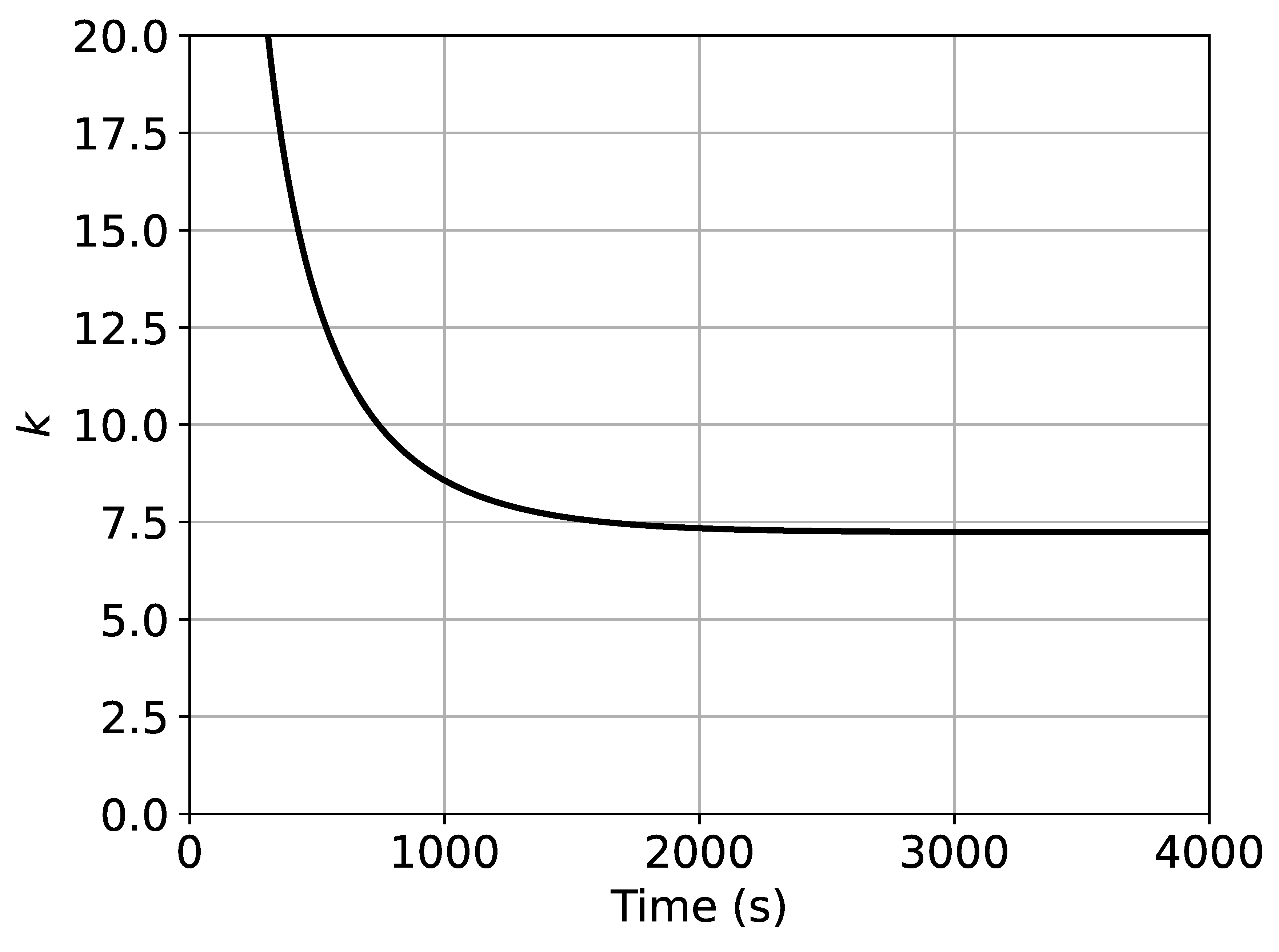
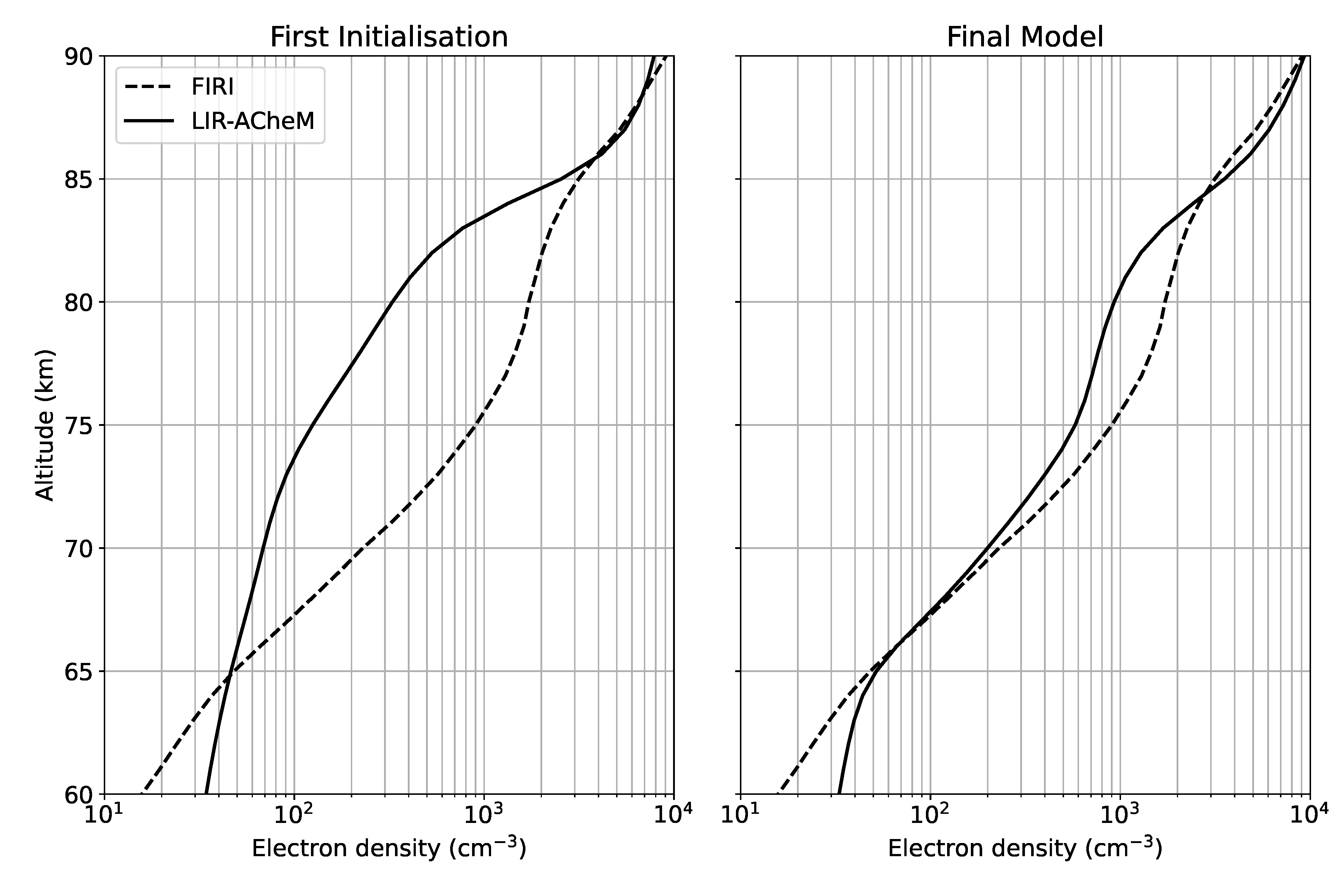
Figure 5.
Variation of k (Equation 13 with time during the first initialisation. This scaling factor is constant after 3000 s, thus defining the time required to initialise the D-region.)
Figure 5.
Variation of k (Equation 13 with time during the first initialisation. This scaling factor is constant after 3000 s, thus defining the time required to initialise the D-region.)
Figure 6.
Comparison of the electron density to FIRI with initial (left) or corrected with scaling factor (right).
Figure 6.
Comparison of the electron density to FIRI with initial (left) or corrected with scaling factor (right).
- above 85 km, dominated by and ;
- between 82 km and 85 km, defined by strong gradients;
- between 70 km and 82 km, characterised by a nearly constant electron density and the presence of water clusters (included through );
- below 70 km, where negative ions are important.
The results presented in Figure 7 showed good agreement for most species with published results [48]. Once the initial ionosphere is set, time-varying external sources may be applied to model the density time evolution during perturbed times (Figure 7, for example, shows the densities at a peak of an M1 flare). This new chemistry model is named the Lower Ionospheric Region – Absorption and Chemistry Modelling (LIR-ACheM). On a personal laptop, modelling the response to a flare takes about a quarter of an hour, with about 90% due to the ionosphere initialisation.
3. D-Region Response to a Flare
In the following, the D-region response to a short M1 solar flare occurring on 2023/11/05 and peaking at 11:43 UT is analysed. The modelling is run at a latitude of 42° and a longitude of 9° to study the D-region behaviour at middle latitudes. One important aspect of the D-region response to a flare is the time between the X-ray peak and the electron density peak, named slugishness and denoted [49,50,51,52,53,54]. Indeed, the ionisation of neutral species is not instantaneous, and occurs with a small-time delay. Appleton [49] showed that
with the effective recombination rate. varies with latitude and season [53], and more importantly, with altitudes (Figure 8). Here, (resp. ) denotes the delay between the SXR (resp. HXR) peak and the electron density modelled at each altitude. As presented in [54], is always higher than , as the HXR peaks before the SXR. Figure 9 shows the computed variation with altitude, and displays the same variation with altitude observed in Figure 5.b. of [52], though the values are higher. In Equation 14, is evaluated at the flux peak. Figure 9 highlights the importance of defining this peak flux: the reference should be the HXR below 85 km and the SXR above this altitude.
Another important metric for the D-region’s response to a solar flare is its recovery time , defined as the time for the electron density to decrease to half its peak value. It is height-dependent, as seen in Figure 8. Three areas defining both and are defined:
- Above 85 km, with a of less than a minute and of a few minutes, decreasing with height,
- Between 70 km and 85 km, where and increase with altitude,
- Below 70 km, with longer and , decreasing with altitudes.
First, at low altitudes, the main source of electrons is not the photoionisation of neutral species, but the detachment of electrons from (Figure 10). This detachment operates on longer timescales than the direct ionisation by solar radiation. The creation of negative ions by attachment and subsequent release of electrons by detachment is thus perceived as a longer recovery, because the electron production by detachment is an additional source of ionisation and reaches its peak after the XR flux. This also causes a rise in .
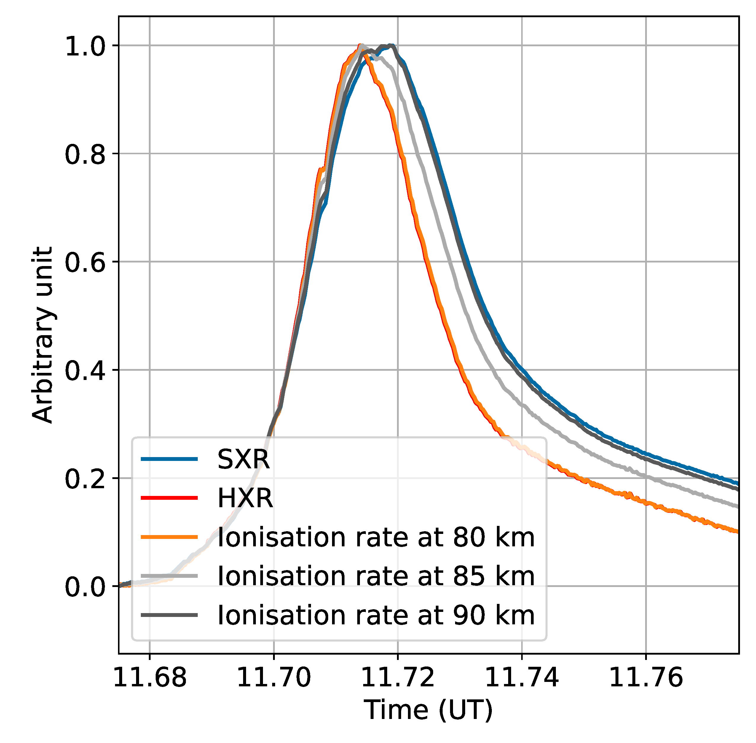
Above 80 km, the SXR flux is not completely absorbed. This is important, as the ionisation cross-sections for SXR wavelengths are much higher than those for the HXR fluxes (Appendix A in the appendix), and the SXR flux is approximately one order of magnitude above the HXR flux. A part of the ionisation at those altitudes is thus due to the SXR flux. A consequence of this is a rise in above 80 km, as the SXR peak occurs after the HXR (e.g. [54] and Figure 11). At 85 km, the ionisation rises with the (early) HXR flux, and falls with the (late) SXR flux. Thus, the perceived is longer, and increases.
Above 85 km, drops with altitude. At those altitudes, the main source of electrons is from the SXR flux (Figure 11). The peak of ionisation occurs later as the ionisation profile starts to follow the SXR flux. thus decreases, as the electron density responds to SXR only. Another factor to explain the altitude variation of is the high at high altitude. Indeed, at 85 km and above, one of the main electron sinks is the recombination with . A higher thus entails lower and as recombination occurs faster.
4. Discussion and Conclusions
A new chemistry model is presented here, LIR-ACheM, based on the Mitra-Rowe scheme. The LIR-ACheM model’s only required inputs are the geographic latitude and longitude, the time, and the forcing (given by the index for the EUV fluxes, the SXR flux in the band 0.1 - 0.8 nm and the HXR flux in the 0.05 - 0.4 nm band, as is given in the GOES data files). Those parameters are used to define the background neutral profiles and the ionisation rates. The outputs contain the variations of the different electron and ion densities for the duration of the modelling, as well as the scaling parameter k for .
Through this model, two important characteristics of the D-region response to solar flares were analysed: the peak delay and the recovery time . Both were found to follow similar altitude profiles. At low altitudes, the main source of electrons is due to a photodetachment. This implies longer and apparent , as this reaction operates on longer timescales. At higher altitudes, however, the ionisation by SXR becomes relevant. At the top of the D-region, it results in a longer apparent at 85 km, which decreases with altitude.
Further improvements in the model include adding more forcing sources (especially the scattering of Lyman- radiation by the Earth’s geocorona, which is dominant in nighttime, and the forcing from electron precipitations for high latitudes). This model is mainly limited in altitude by the production rate of from EUV, parametrised by Paulsen et al. [36]. Another description of this rate could therefore extend the validity of this model to higher altitudes.
The user is free to provide their own neutral background. This model version (v1.3.1) indeed initialises the background neutral atmosphere from NRLMSISE-00 by default. [55] showed that using a different neutral background causes deviations in the computed electron density of the order of 34%. In the present study, the initialisation of the background was done, for example, through the NRLMSISE-2.1 model and the various references presented in Section 2.1.
Author Contributions
Conceptualization, C. Briand. and P. Teysseyre.; Software, P. Teysseyre; Writing – Original Draft Preparation, C.Briand. and P.Teysseyre.; Supervision, C. Briand”
Funding
The CNRS supported the present work through its PNST/ATST program, as well as the CSAA. The CNES also supported this work through its support to Space Weather programs.
Data Availability Statement
The LIR-ACheM model is available at https://codeberg.org/pteysseyre/LIR-ACheM . Before the paper is accepted, the model is only available through Codeberg with the username `lirachem_collaborator’ and password `LIRACHEM’.
Acknowledgments
Conflicts of Interest
The authors declare no conflicts of interest.
Abbreviations
The following abbreviations are used in this manuscript:
| VLF | Very Low Frequency |
| HF | High Frequency |
| SXR | Soft X-ray (0.1 - 0.8 nm) |
| HXR | Hard X-ray (0.05 - 0.4 nm) |
| EUV | Extreme Ultraviolet (102.7 - 111.8 nm) |
| CR | Cosmic rays |
| GOES | Geostationary Operational Environmental Satellite |
| XR | X-rays |
Appendix A
This section gives more details on the computation of the different ionisation terms
Appendix A.1. Chapman Function
Appendix A.2. Absorption and Ionisation Cross Sections
The absorption of the different wavelengths is due to the major species O, and (e.g., [43,45]). The absorption cross-sections are represented in Table A1.

Table A1.
Absorption cross-sections (, cm2) of the main neutral species , and O [43].
Table A1.
Absorption cross-sections (, cm2) of the main neutral species , and O [43].
| SXR (0.1-0.8 nm) | HXR (0.05-0.4 nm) | |
|---|---|---|
| 0.0201 | 0.0025 | |
| 0.0340 | 0.0045 | |
| O | 0.0170 | 0.0023 |
The Lyman- radiation, however, is mainly absorbed by [57]. The mean absorption cross-section is given by:
where the neutral temperature is in K and .
If the HXR range is discretised in 0.05 nm bins, then the cross-sections need to be adapted. They are presented in Table A2.
Table A2.
Absorption cross-sections ( ) of the main neutral species , and O for different wavelengths in the HXR range [40].
Table A2.
Absorption cross-sections ( ) of the main neutral species , and O for different wavelengths in the HXR range [40].
| Wavelength (nm) | O | ||
|---|---|---|---|
| 0.05-0.10 | |||
| 0.10-0.15 | |||
| 0.15-0.20 | |||
| 0.20-0.25 | |||
| 0.25-0.30 | |||
| 0.30-0.40 |
In Equation 7, represents the ionisation cross-section of species n. This ionisation comes from the direct interaction of solar radiation with the neutral species. This interaction can result in ionisation, dissociation or dissociative ionisation, and the ratio between each of those possibilities is called the branching ratio. Specifically, is the branching ratio for ionisation. Those values are tabulated in [40,43], so that:
Appendix A.3. Computation of k λ
In [43], the value of the ratio of photoelectron impact ionisation to ionisation by external sources is given for the three major neutral species, for different wavelengths. Here, . The values are later reevaluated by [40], for narrower HXR bins, and range between 66 and 554. Most of the D-region ionisation during flares thus comes from electron impact ionisation.
Appendix B. Reaction Rates in the Mitra-Rowe Scheme
The different reaction rates in the Mitra-Rowe scheme are presented in Table A3. corresponds to and , with in K.
Table A3.
Reaction rates in our implementation of the Mitra-Rowe scheme.
| Reaction | Rate ( or ) | Reference |
|---|---|---|
| A | [13] | |
| B | [13] | |
| [1,13] | ||
| [45] Table 6, Reaction 30 | ||
| [45] Table 6, Reaction 27 | ||
| [45] Table 6, Reaction 110 | ||
| [13] | ||
| [13] | ||
| [45] Table 10, Reaction 26 | ||
| [45] Table 10, Reaction 27 | ||
| [45] Table 10, Reaction 31 | ||
| [45] Table 10, Reaction 33 | ||
| [45] Table 10, Reaction 34 | ||
| 0.1 + | [6] | |
| to | [45] Table 10, Reaction 1 | |
| [45] Table 10, Reaction 2 | ||
| to | [13] | |
| to | [45] Table 6, Reaction 36 | |
| to | [45] Table 6, Reaction 37 | |
| [45] Table 6, Reaction 44 | ||
| [45] Table 6, Reaction 45 | ||
| to | [45], Table 6, Reaction 28] | |
| [45] Table 6, Reaction 29 |
References
- Mitra, A.; Rowe, J. Ionospheric effects of solar flares—VI. Changes in D-region ion chemistry during solar flares. J. Atmos. Terr. Phys. 1972, 34, 795–806. [Google Scholar]
- Reid, G.C. Production and loss of electrons in the quiet daytime D region of the ionosphere. J. Geophys. Res. 1970, 75, 2551–2562. [Google Scholar] [CrossRef]
- McEwan, M.J.; Phillips, L.F. Chemistry of the atmosphere; Halsted Press: New York, 1975. [Google Scholar]
- Ferguson, E.E. Ion-molecule reactions in the atmosphere. In Kinetics of Ion-Molecule Reactions; Springer, 1979; pp. 377–403. [Google Scholar]
- Thomas, L.; Bowman, M. Model studies of the D-region negative-ion composition during day-time and night-time. J. Atmos. Terr. Phys. 1985, 47, 547–556. [Google Scholar] [CrossRef]
- Burns, C.; Turunen, E.; Matveinen, H.; Ranta, H.; Hargreaves, J. Chemical modelling of the quiet summer D- and E-regions using EISCAT electron density profiles. J. Atmos. Terr. Phys. 1991, 53, 115–134. [Google Scholar] [CrossRef]
- Bekker, S.; Ryakhovsky, I.; Korsunskaya, J. Modeling of the lower ionosphere during solar X-ray flares of different classes. J. Geophys. Res. Space Phys. 2021, 126, e2020JA028767. [Google Scholar] [CrossRef]
- Glukhov, V.S.; Pasko, V.P.; Inan, U.S. Relaxation of transient lower ionospheric disturbances caused by lightning-whistler-induced electron precipitation bursts. JGR 1992, 97, 16971–16979. [Google Scholar] [CrossRef]
- Lehtinen, N.G.; Inan, U.S. Possible persistent ionization caused by giant blue jets. Geophys. Res. Lett. 2007, 34. [Google Scholar] [CrossRef]
- Turunen, E.; Matveinen, H.; Tolvanen, J.; Ranta, H. D-region ion chemistry model. STEP Handb. Ionos. Model. 1996, 1–25. [Google Scholar]
- Verronen, P.T.; Andersson, M.E.; Marsh, D.R.; Kovács, T.; Plane, J.M.C. WACCM-D—Whole Atmosphere Community Climate Model with D-region ion chemistry. J. Adv. Model. Earth Syst. 2016, 8, 954–975. [Google Scholar] [CrossRef]
- Rowe, J.; Mitra, A.; Ferraro, A.; Lee, H. An experimental and theoretical study of the D-region—II. A semi-empirical model for mid-latitude D-region. J. Atmos. Terr. Phys. 1974, 36, 755–785. [Google Scholar] [CrossRef]
- Mitra, A. D-region in disturbed conditions, including flares and energetic particles. J. Atmos. Terr. Phys. 1975, 37, 895–913. [Google Scholar] [CrossRef]
- Wait, J.R.; Spies, K.P. Characteristics of the Earth-ionosphere waveguide for VLF radio waves; US Department of Commerce, National Bureau of Standards, 1964; Vol. 13. [Google Scholar]
- Thomson, N. Experimental daytime VLF ionospheric parameters. J. Atmos. Terr. Phys. 1993, 55, 173–184. [Google Scholar] [CrossRef]
- Ferguson, J.A. Computer Programs for Assessment of Long- Wavelength Radio Communications, Version 2.0. Technical document 3030.
- Gasdia, F.; Marshall, R.A. A new longwave mode propagator for the Earth–ionosphere waveguide. IEEE Trans. Antennas Propag. 2021, 69, 8675–8688. [Google Scholar] [CrossRef]
- Emmert, J.T.; Jones, M.; Siskind, D.E.; Drob, D.P.; Picone, J.M.; Stevens, M.H.; Bailey, S.M.; Bender, S.; Bernath, P.F.; Funke, B.; et al. NRLMSIS 2.1: An Empirical Model of Nitric Oxide Incorporated Into MSIS. J. Geophys. Res. Space Phys. 2022, 127, e2022JA030896. [Google Scholar] [CrossRef]
- Picone, J.; Hedin, A.; Drob, D.P.; Aikin, A. NRLMSISE-00 empirical model of the atmosphere: Statistical comparisons and scientific issues. J. Geophys. Res. Space Phys. 2002, 107, SIA–15. [Google Scholar] [CrossRef]
- Crutzen, P.; Jones, I.; Wayne, R. Calculation of [O2 (1Δg)] in the atmosphere using new laboratory data. J. Geophys. Res. 1971, 76, 1490–1497. [Google Scholar] [CrossRef]
- Barth, C.A. Rocket measurement of nitric oxide in the upper atmosphere. Planet. Space Sci. 1966, 14, 623–630. [Google Scholar] [CrossRef]
- Pearce, J.B. Rocket measurement of nitric oxide between 60 and 96 kilometers. J. Geophys. Res. 1969, 74, 853–861. [Google Scholar]
- Gylvan Meira, L., Jr. Rocket measurements of upper atmospheric nitric oxide and their consequences to the lower ionosphere. J. Geophys. Res. 1971, 76, 202–212. [Google Scholar] [CrossRef]
- Baker, K.; Nagy, A.; Olsen, R.; Oran, E.; Randhawa, J.; Strobel, D.; Tohmatsu, T. Measurement of the nitric oxide altitude distribution in the mid-latitude mesosphere. J. Geophys. Res. 1977, 82, 3281–3286. [Google Scholar] [CrossRef]
- Grossmann, K.; Frings, W.; Offermann, D.; André, L.; Kopp, E.; Krankowsky, D. Concentrations of H2O and NO in the mesosphere and the lower thermosphere at high latitudes. J. Atmos. Terr. Phys. 1985, 47, 291–300. [Google Scholar] [CrossRef]
- Mitra, A.P. An ionospheric estimate of nitric oxide concentration in the D-region. J. Atmos. Terr. Phys. 1966, 28, 945–955. [Google Scholar] [CrossRef]
- Hesstvedt, E.; Jansson, U.B. A photochemical atmosphere model containing oxygen, hydrogen, and nitrogen; Technical report; Oslo Institute Norway Institute Geophysics, 1969. [Google Scholar]
- Rusch, D.W.; Sharp, W.E. Nitric oxide delta band emission in the earth’s atmosphere: Comparison of a measurement and a theory. J. Geophys. Res. Space Phys. 1981, 86, 10111–10114. [Google Scholar] [CrossRef]
- Fabian, P.; Pyle, J.; Wells, R. Diurnal variations of minor constituents in the stratosphere modeled as a function of latitude and season. J. Geophys. Res. Ocean. 1982, 87, 4981–5000. [Google Scholar] [CrossRef]
- Torkar, K.; Friedrich, M. Tests of an ion-chemical model of the D-and lower E-region. J. Atmos. Terr. Phys. 1983, 45, 369–385. [Google Scholar] [CrossRef]
- Reid, G.C. The roles of water vapor and nitric oxide in determining electron densities in the D-region. In Proceedings of the Mesospheric Models and Related Experiments: Proceedings of the Fourth Esrin-Eslab Symposium Held in Frascati, Italy, 6–10 July, 1970; Springer, 1971; pp. 198–209. [Google Scholar]
- Torr, D.G. The photochemistry of the upper atmosphere. Photochem. Atmos. Earth 1985, 165–278. [Google Scholar]
- Bland, E.; Tesema, F.; Partamies, N. D-region impact area of energetic electron precipitation during pulsating aurora. Ann. Geophys. 2021, 39, 135–149. [Google Scholar] [CrossRef]
- Rodriguez, J.V.; Inan, U.S.; Bell, T.F. D region disturbances caused by electromagnetic pulses from lightning. Geophys. Res. Lett. 1992, 19, 2067–2070. [Google Scholar] [CrossRef]
- Watanabe, K.; Matsunaga, F.M.; Sakai, H. Absorption coefficient and photoionization yield of NO in the region 580–1350 Å. Appl. Opt. 1967, 6, 391–396. [Google Scholar] [CrossRef]
- Paulsen, D.; Huffman, R.; Larrabee, J. Improved photoionization rates of O2 (1Δg) in the D region. Radio Sci. 1972, 7, 51–55. [Google Scholar]
- Richards, P.G.; Fennelly, J.A.; Torr, D.G. EUVAC: A solar EUV Flux Model for aeronomic calculations. J. Geophys. Res. Space Phys. 1994, 99, 8981–8992. [Google Scholar] [CrossRef]
- Nicolet, M.; Aikin, A. The formation of the D region of the ionosphere. J. Geophys. Res. 1960, 65, 1469–1483. [Google Scholar] [CrossRef]
- Bourdeau, R.E.; Aikin, A.C.; Donley, J.L. Lower ionosphere at solar minimum. J. Geophys. Res. 1966, 71, 727–740. [Google Scholar] [CrossRef]
- Siskind, D.E.; Jones, M., Jr.; Reep, J.W.; Drob, D.P.; Samaddar, S.; Bailey, S.M.; Zhang, S.R. Tests of a New Solar Flare Model Against D and E Region Ionosphere Data. Space Weather 2022, 20, e2021SW003012. [Google Scholar] [CrossRef]
- Singer, S. Physics of the Upper Atmosphere. John A. Ratcliffe, Ed. Academic Press, New York, 1960. 586 pp. In Illus. Science; 1961; Volume 133, pp. 1123–1124. [Google Scholar]
- Brasseur, G.P.; Solomon, S. Aeronomy of the middle atmosphere: Chemistry and physics of the stratosphere and mesosphere; Springer, 2005. [Google Scholar]
- Solomon, S.C.; Qian, L. Solar extreme-ultraviolet irradiance for general circulation models. J. Geophys. Res. Space Phys. 2005, 110. [Google Scholar] [CrossRef]
- Hargreaves, J.K. The solar-terrestrial environment. An introduction to geospace - the science of the terrestrial upper atmosphere, ionosphere and magnetosphere. Camb. Atmos. Space Sci. Ser. 1992, 5. [Google Scholar]
- Pavlov, A. Photochemistry of ions at D-region altitudes of the ionosphere: A review. Surv. Geophys. 2014, 35, 259–334. [Google Scholar]
- Friedrich, M.; Pock, C.; Torkar, K. FIRI-2018, an Updated Empirical Model of the Lower Ionosphere. J. Geophys. Res. Space Phys. 2018, 123, 6737–6751. [Google Scholar] [CrossRef]
- Mitra, A. Chemistry of middle atmospheric ionization—a review. J. Atmos. Terr. Phys.;Equat. Aeron.-II 1981, 43, 737–752. [Google Scholar] [CrossRef]
- Reid, G.C. The middle atmosphere. In Proceedings of the Middle Atmosphere Electrodynamics; Maynard, N.C., Ed.; 1979; pp. 27–42. [Google Scholar]
- Appleton, E.V. A note on the “sluggishness” of the ionosphere. J. Atmos. Terr. Phys. 1953, 3, 282–284. [Google Scholar] [CrossRef]
- Žigman, V.; Grubor, D.; Šulić, D. D-region electron density evaluated from VLF amplitude time delay during X-ray solar flares. J. Atmos. Sol.-Terr. Phys. 2007, 69, 775–792. [Google Scholar] [CrossRef]
- Basak, T.; Chakrabarti, S.K. Effective recombination coefficient and solar zenith angle effects on low-latitude D-region ionosphere evaluated from VLF signal amplitude and its time delay during X-ray solar flares. Astrophys. Space Sci. 2013, 348, 315–326. [Google Scholar] [CrossRef]
- Palit, S.; Basak, T.; Pal, S.; Chakrabarti, S.K. Theoretical study of lower ionospheric response to solar flares: sluggishness of D-region and peak time delay. Astrophys. Space Sci. 2015, 356, 19–28. [Google Scholar] [CrossRef]
- Chakraborty, S.; Paul, R.; Basak, T. On the altitude profile of lower ionospheric D-region response time delay during solar flares. Front. Environ. Sci. 2022, 10, 1020137. [Google Scholar] [CrossRef]
- Briand, C.; Clilverd, M.; Inturi, S.; Cecconi, B. Role of hard X-ray emission in ionospheric D-layer disturbances during solar flares. Earth Plan. Space 2022, 74, 41. [Google Scholar] [CrossRef]
- Bekker, S.Z.; Korsunskaya, J.A. Influence of the Neutral Atmosphere Model on the Correctness of Simulation the Electron and Ion Concentrations in the Lower Ionosphere. J. Geophys. Res. Space Phys. 2023, 128, e2023JA032007. [Google Scholar] [CrossRef]
- Smith, F.L., III; Smith, C. Numerical evaluation of Chapman’s grazing incidence integral ch (X, χ). J. Geophys. Res. (1896-1977) 1972, 77, 3592–3597. [Google Scholar] [CrossRef]
- Reddmann, T.; Uhl, R. The H Lyman-. α Actinic Flux Middle Atmos. 2002. [Google Scholar] [CrossRef]
Figure 1.
Neutral profiles for the initialisation of the D-region.
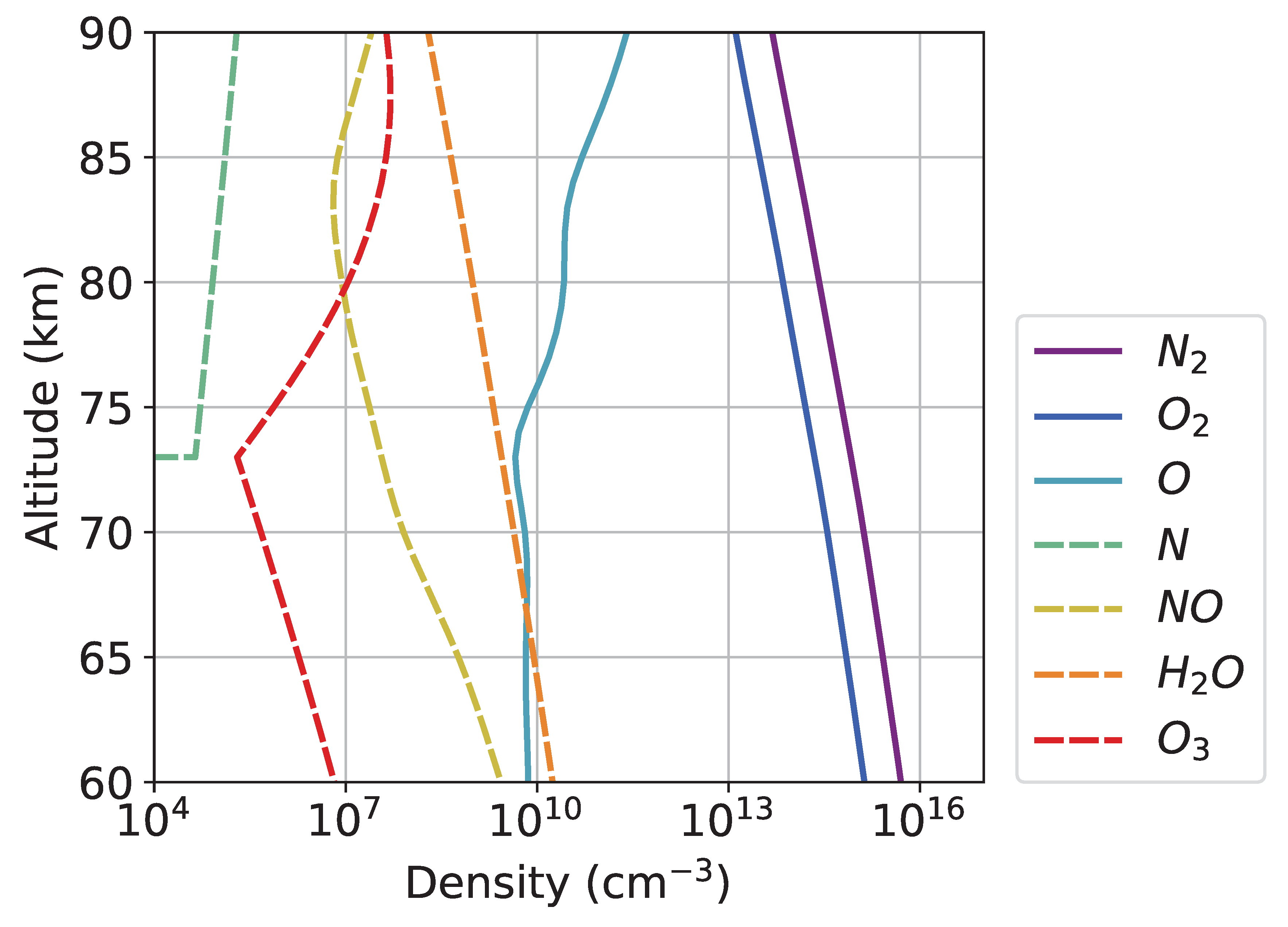
Figure 2.
Transmission factor for different wavelengths. This closely matches Figure 25 of [41], p.186].
Figure 2.
Transmission factor for different wavelengths. This closely matches Figure 25 of [41], p.186].
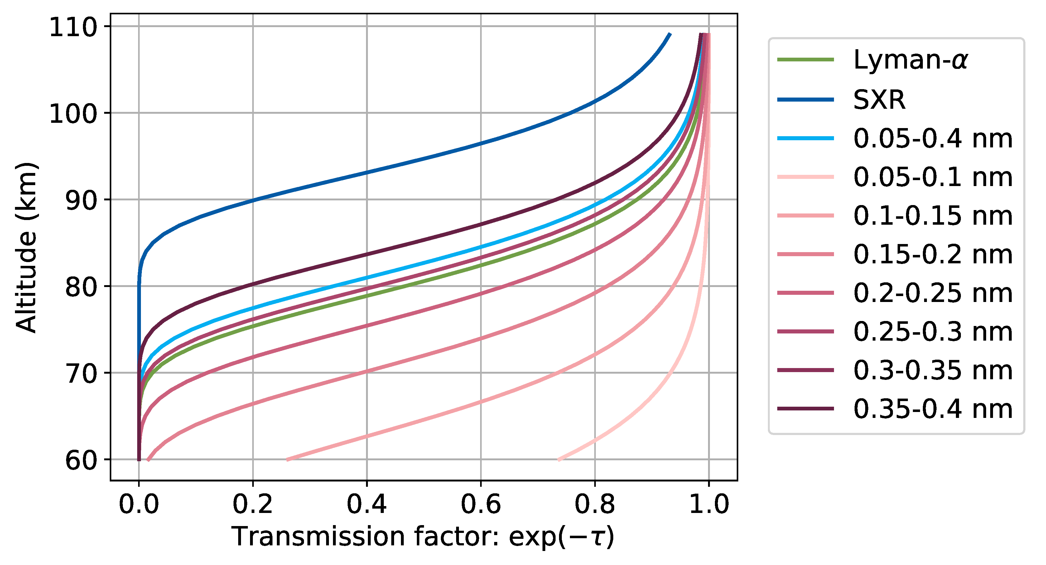
Figure 3.
Ionisation rates from the various ionisation sources vs altitude during quiet times (left) or during an M1 flare (right). The control of the D-region during quiet times by the ionisation of by Lyman- radiation [1,4,5,6] is recovered, while the ionisation by XR is important mainly during flares. The species involved in each ionisation term are specified in parentheses in the legend.
Figure 3.
Ionisation rates from the various ionisation sources vs altitude during quiet times (left) or during an M1 flare (right). The control of the D-region during quiet times by the ionisation of by Lyman- radiation [1,4,5,6] is recovered, while the ionisation by XR is important mainly during flares. The species involved in each ionisation term are specified in parentheses in the legend.
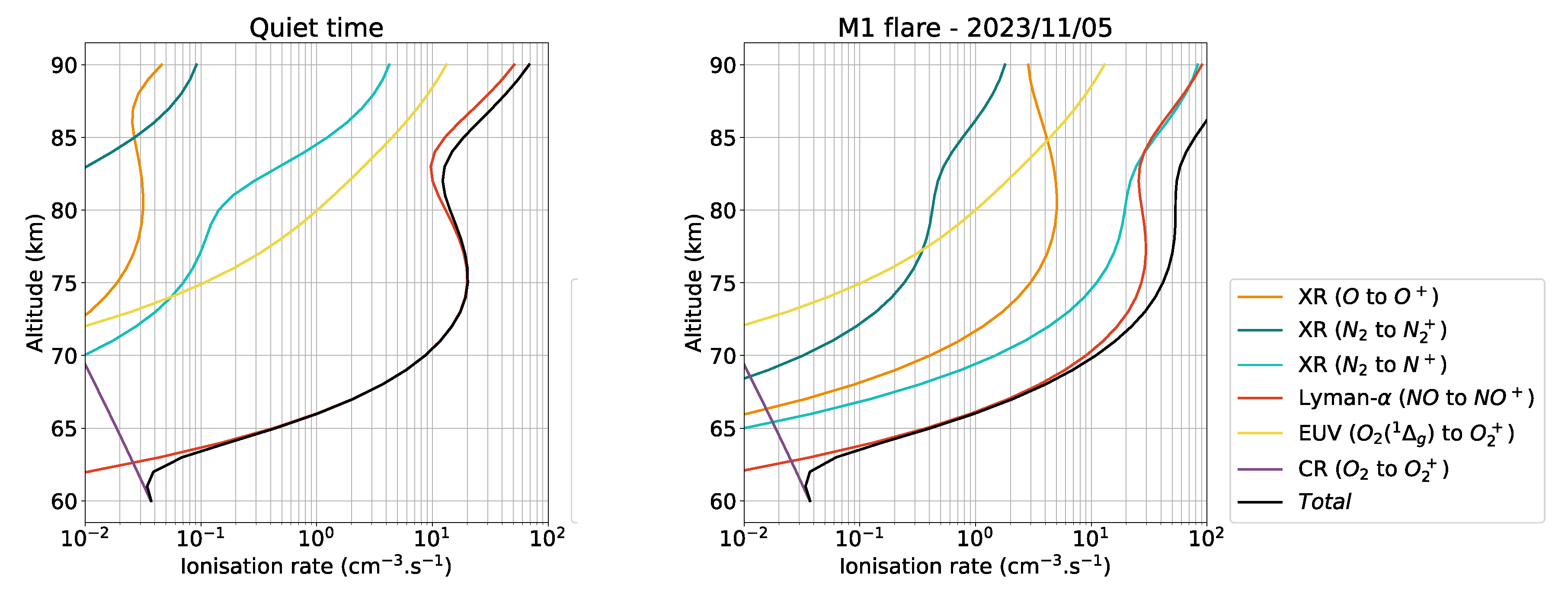
Figure 4.
Mitra-Rowe scheme. represents positive clusters, while denotes every negative ion except . The details of the various coefficients are given in Appendix B of the appendix.
Figure 4.
Mitra-Rowe scheme. represents positive clusters, while denotes every negative ion except . The details of the various coefficients are given in Appendix B of the appendix.
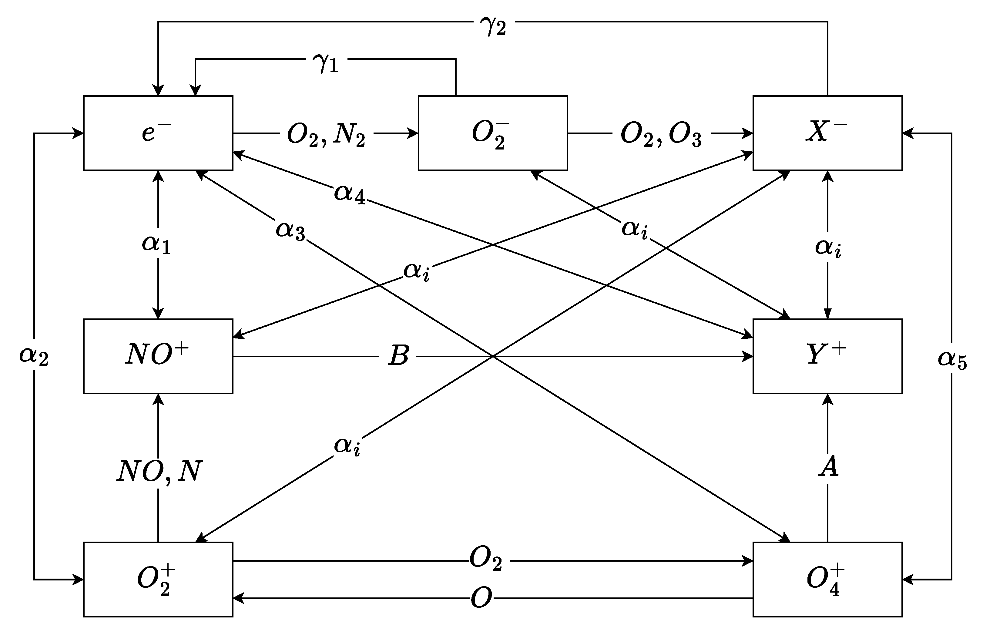
Figure 7.
Ion profiles in quiet time (left) and at the peak of an M1 flare (right), on 2023/11/05 (). The horizontal lines separate the four areas described in [47] and presented in the text.
Figure 7.
Ion profiles in quiet time (left) and at the peak of an M1 flare (right), on 2023/11/05 (). The horizontal lines separate the four areas described in [47] and presented in the text.
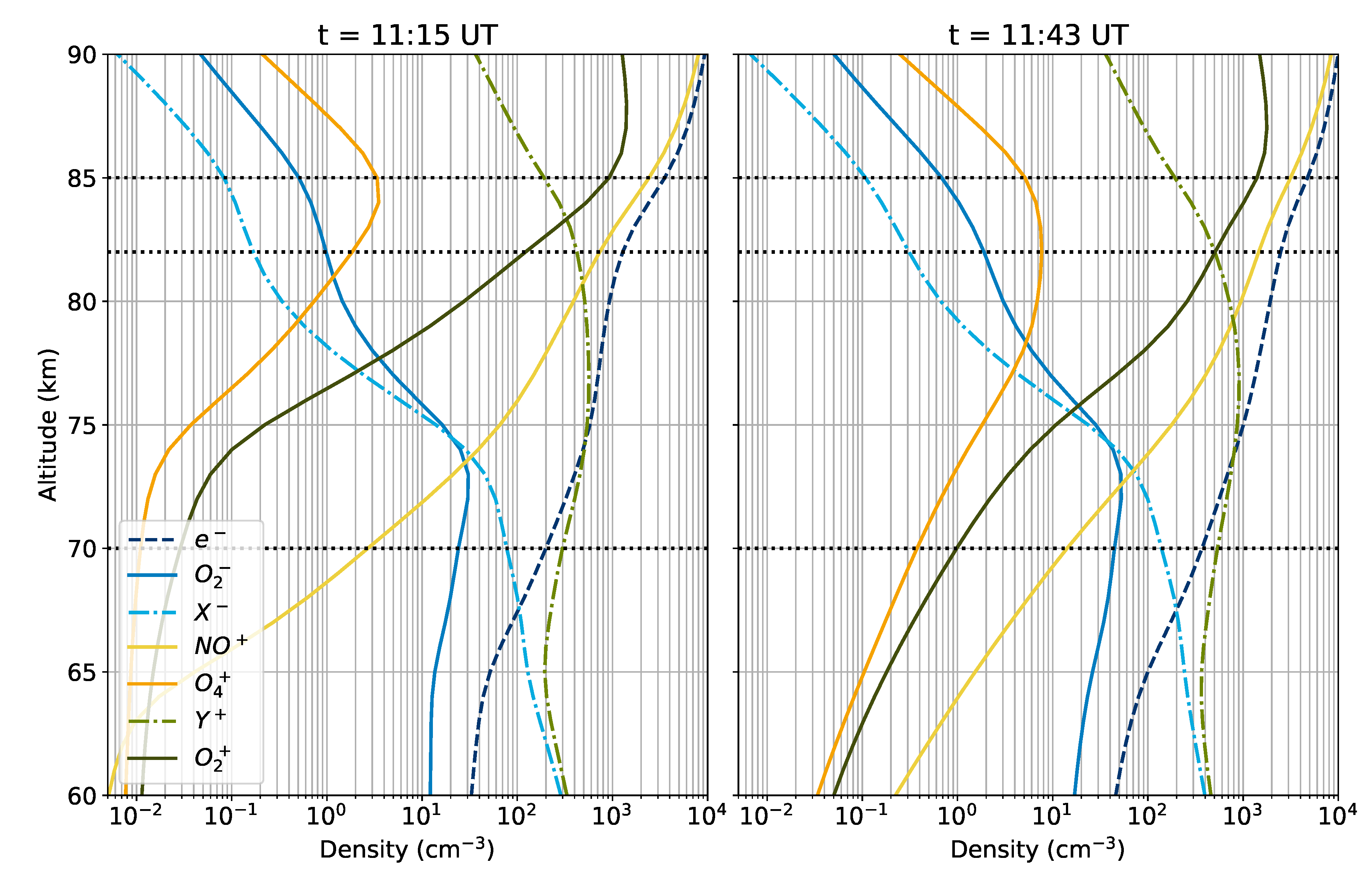
Figure 8.
(orange) and (blue) vs altitude after the M1 flare occurring on 2023/11/05 at 11:43 UT. was computed respectively to the HXR peak (, dashed lines) and the SXR peak (, plain line).
Figure 8.
(orange) and (blue) vs altitude after the M1 flare occurring on 2023/11/05 at 11:43 UT. was computed respectively to the HXR peak (, dashed lines) and the SXR peak (, plain line).
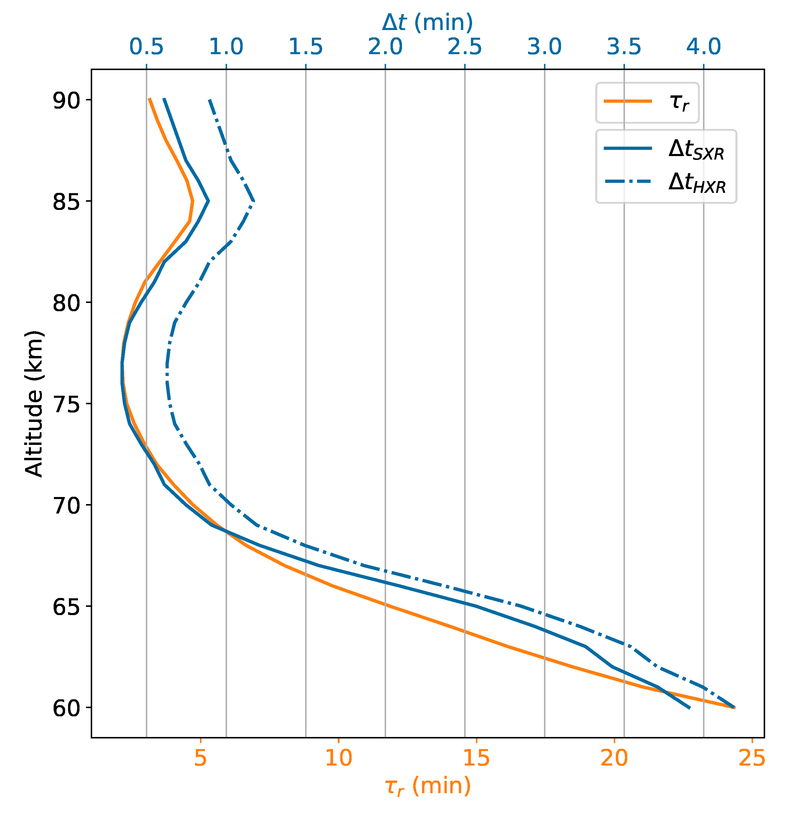
Figure 9.
vs altitude. depends explicitely on (Equation 14). However, is computed as the delay between the either the SXR or the HXR peak and the electron density peak. The resulting are represented in blue and orange respectively.
Figure 9.
vs altitude. depends explicitely on (Equation 14). However, is computed as the delay between the either the SXR or the HXR peak and the electron density peak. The resulting are represented in blue and orange respectively.
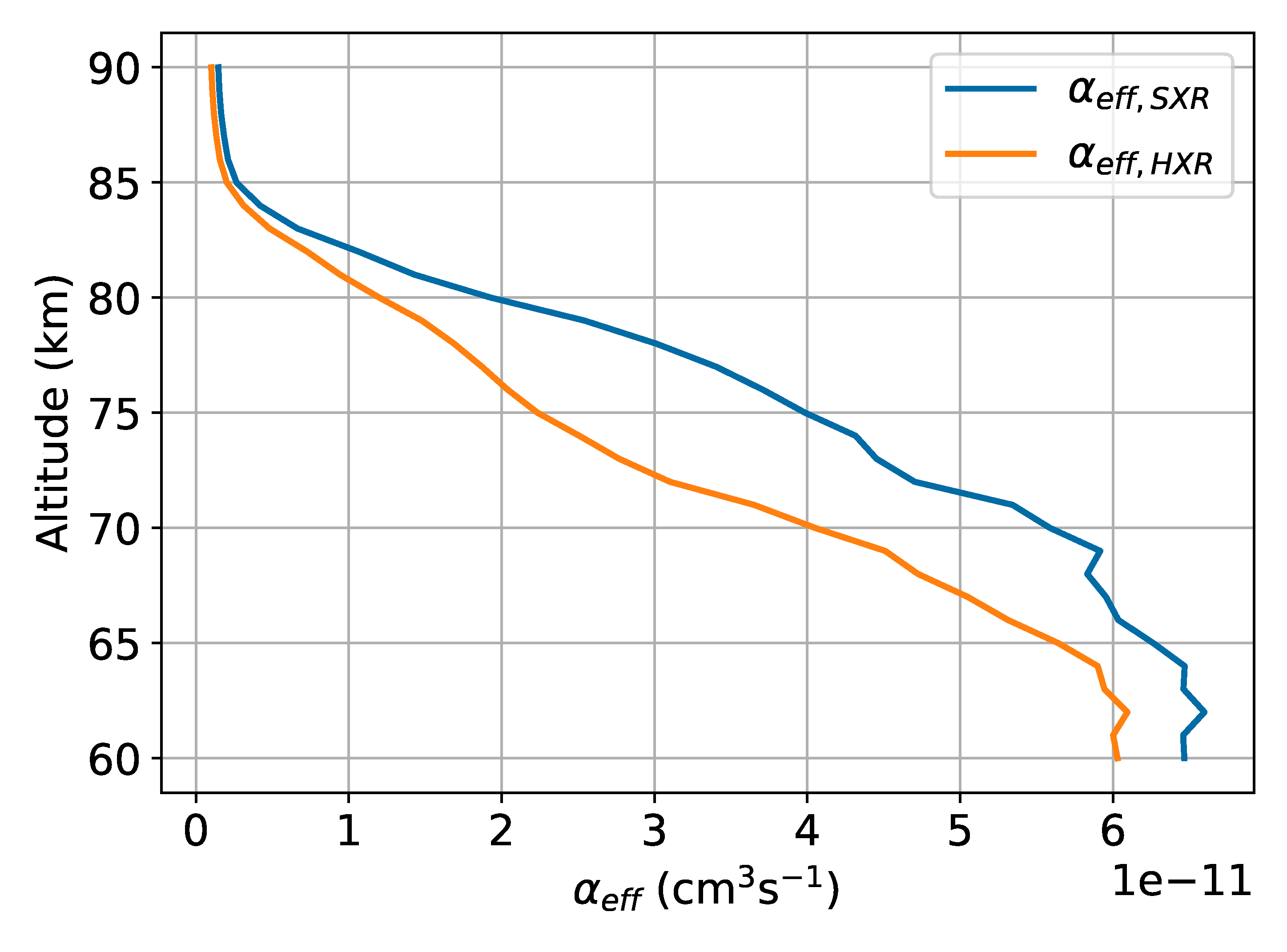
Figure 10.
Relative importance of the electron sources with altitudes in quiet time. At high altitude, the electrons are mostly created by external forcing. At low altitudes, however, their level is maintained by the detachment from negative ions, which act as a bank of electrons.
Figure 10.
Relative importance of the electron sources with altitudes in quiet time. At high altitude, the electrons are mostly created by external forcing. At low altitudes, however, their level is maintained by the detachment from negative ions, which act as a bank of electrons.
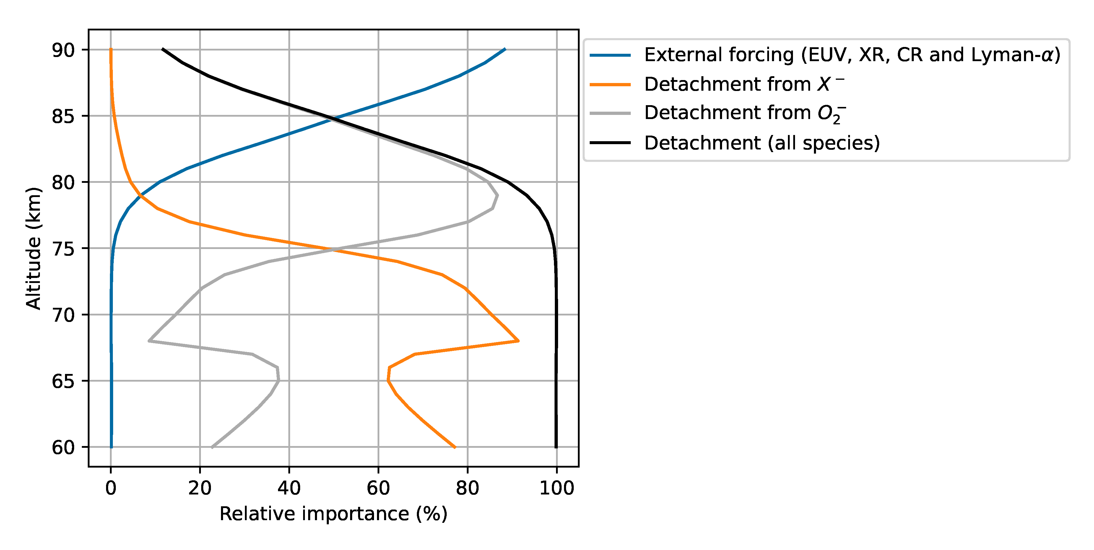
Figure 11.
SXR (blue) and HXR (red) fluxes vs time. The total ionisation at 80 (orange), 85 (light grey) and 90 km (dark grey) is presented. All curves have been normalised for better visibility.
Figure 11.
SXR (blue) and HXR (red) fluxes vs time. The total ionisation at 80 (orange), 85 (light grey) and 90 km (dark grey) is presented. All curves have been normalised for better visibility.
Disclaimer/Publisher’s Note: The statements, opinions and data contained in all publications are solely those of the individual author(s) and contributor(s) and not of MDPI and/or the editor(s). MDPI and/or the editor(s) disclaim responsibility for any injury to people or property resulting from any ideas, methods, instructions or products referred to in the content. |
© 2026 by the authors. Licensee MDPI, Basel, Switzerland. This article is an open access article distributed under the terms and conditions of the Creative Commons Attribution (CC BY) license.
Copyright: This open access article is published under a Creative Commons CC BY 4.0 license, which permit the free download, distribution, and reuse, provided that the author and preprint are cited in any reuse.


