

Submitted:
01 May 2026
Posted:
06 May 2026
You are already at the latest version
Abstract
A covariant formulation of the Geometric Dilution of Precision (GDOP) matrix is presented in the framework of a Relativistic Positioning System (RPS). By including the receiver-emitter frequency ratios, the Frequency Geometric Dilution of Precision (FGDOP) scalar is computed in terms of observable quantities, the received frequencies and the angular separation between pairs of emitters in view. Some required concepts are first introduced: the FGDOP matrix and the Gram matrix associated to k light-like vectors. From the tensor form of the FGDOP matrix and its trace, a closed form of the FGDOP scalar is obtained, extending previous matrix calculations. Clarifying computations for symmetric emitter configurations are presented. The geometric interpretation of the GDOP scalar in terms of volumes and areas defined by the relative position of the emitters on the unit celestial sphere of the user is also recovered.
Keywords:
relativistic positioning systems
; frequency geometric dilution of precision
; covariant approach
1. Introduction
The term Geometric Dilution of Precision (GDOP) is widely used in the context of Global Navigation Satellite Systems (GNSSs). It refers to a matrix constructed from the positions of the satellites on the sky, the GDOP matrix, as well as to the square root of its trace, the so called GDOP scalar. The latter is a dimensionless metric indicator of the goodness in the determination of the user location from the geometry of the satellite configuration in view, assuming a simple stochastic model [1,2,3].
More specifically, the classical positioning approach usually applies the least squares method to minimize the differences between modelled emitter-receiver distances and measured pseudoranges (travel times multiplied by the signal velocity). For k satellites in view at the user location, the GDOP matrix is the matrix defined as the inverse of , where denotes the transpose of H, the matrix whose Ath row is , with the unit vector along the line of sight of the A-emitter () expressed in Cartesian coordinates [1,2,3].
Then, under the hypothesis of unbiased and independent measurement errors, the root mean square error of the estimated user location is directly proportional to the GDOP scalar, the proportionality factor being the (square root of the) variance of the measurements. Therefore, the lower the value of the GDOP scalar, the more favorable the satellite configuration will be to attain an accurate user location and dismiss the consequences of measurement errors. High GDOP scalar values are commonly associated to bad or degenerate satellite distributions unfavourable to an effective user localization. Furthermore, as shown in [4], when the stochastic model for the pseudorange measurements is supposed Gaussian, the Cramer-Rao lower bound in estimating the user position and clock offset is reached by the GDOP matrix.
The GDOP terminology also applies in other location situations, for instance, to guide unmanned vehicles with precision. In this case the GDOP matrix involves the unit vectors pointing towards the vehicle from a station network or a set of spatially separated sensors [5,6].
The algebraic approach to GDOP concepts was analyzed and discussed by diverse authors as soon as the pioneering Global Positioning System (GPS) project was announced [7,8,9,10,11,12]. The GDOP scalar has been expressed in terms of tetrahedron volumes and triangle surfaces constructed from the unit vectors along the direction of the received signals from the emitters to the user [13,14,15]. As proposed in [16,17], the (weighted and non-weighted) GDOP scalar can be computed from the traces of powers of the so-called geometric matrix, which is explicitly carried out in the present work.
By selecting favorable sets of satellites in view, collaboration between current GNSSs should ensure positioning accuracy for a passive network of receptors. The starting point for satellite selection criteria is the GDOP computation or their variants (weighted GDOP) with additional information from a network of satellites other than the sky configuration. In [6] the authors combine GDOP and weighted GDOP computations and near-real-time observation accuracy as a satellite selection method improving other methods based on signal-to-noise ratios. In this paper, we propose a new GDOP study, a fully relativistic one which introduces the received-emitted frequency ratio as additional (non-geometric) system information. Formally, this frequency ratio can operate as a traditional weight in extended GDOP computations, informing about the effect of Doppler shifts on the degree of positioning precision. Nevertheless, the GDOP approach here presented differs from the classical one in the sense that the theory of relativity is fundamental to introduce, justify and interpret the concepts involved. The frequency-weighted extended GDOP is a useful tool to improve existing satellite selection methods, either by numerically implementing the covariant equation (1) given in Section 2 or the geometric equation (84) given in Section 6.
Nevertheless, the primordial objective of this work is to adapt the current classical GDOP formalism to the theory of Relativistic Positioning Systems (RPSs). In fact, the determination of the user location based on pseudorange measurements by common GNSS receivers [1,3] does not take into account frequency measurements, which are otherwise necessary to determine the user velocity with high accuracy or the position in unfavorable situations [18]. In this regard, the deployment of Low Earth Orbit (LEO) satellites has recently motivated the related notion of Doppler GDOP (DGDOP) [19,20,21].
The essential ingredients of a RPS are four emitter world-lines broadcasting their respective proper times (or any other time scale) by means of electromagnetic signals. The set of four broadcast times are the emission coordinates of the RPS, which are natural coordinates numbering the emitters’ future-oriented null cones [22]. Emission coordinates admit Newtonian analogous constructions broadcasting sound signals [23]. In [24] it was outlined that in the region where a RPS operates, any event knows its own coordinates immediately (that is, without delay); besides, the physical realization of a RPS does not require prior knowledge of the gravitational field and can therefore operate in any space-time. That is, at any space-time region, the realization of a RPS allows to construct a primary reference system, opening the possibility to make gravimetry, as shown in two-dimensional Lorentzian space-times [24,25,26]. The idea to develop gravimetry under the perspective of RPS theory [27] has motivated an extended classification of the properties required for a RPS [28,29]. On the other hand, emission coordinates have also been studied in [30] using the term GPS coordinates previously introduced in [31,32,33].
For an account of the genesis and current status of RPS theory see [27,31,34,35]. The main ambitious objective of RPS theory is to construct a truly relativistic laboratory with full self-capabilities to perform gravimetry in an unknown space-time region [35]. The interest of RPS theory in GNSS was stressed in [22,31]; it pursues the construction of a global reference system, primarily based on the sky sector (satellites), providing accurate positioning and time localization of the actions of control stations. The transformation from emission to inertial coordinates [36] provides the location of the user in flat space-time, once the emission coordinate domains have been analyzed in relation to the bifurcation problem [37,38,39,40]. Numerical implementation of this transformation in GNSS systems has been proposed in [41,42,43,44]. Numerical positioning simulations in Schwarzschild and perturbed Schwarzschild space-time have been performed in [34,45].
To attain a relativistic formulation of the GDOP, as an alternative to the Newtonian conception on which current notion is rooted, some aspects have to be investigated further. The search for a fully relativistic treatment of the GDOP must consider at least two main tasks: (i) to establish a covariant GDOP formalism, based on relativistic terminology, and (ii) to develop a 3+1 formulation for the GDOP, relative to an arbitrary observer, in the framework of RPS theory [39]. The present work is mainly focused on the first task (i). The results here achieved pave the way to develop the second and complementary task (ii), which is discussed in [46].
This paper is organized in steps to reach formula (1) advanced in Section 2, which allows to evaluate the so-called Frequency GDOP (FGDOP) scalar from observable quantities (the receiver-emitter frequency ratios and the angular separation between pairs of emitters). The required concepts are introduced in due time: The notion of emission coordinates (of the broadcast proper times) and its gradients are explained in Section 3, showing the relation between the GDOP and the Jacobian determinant of the transformation from inertial to emission coordinates. The Frequency-Geometric matrix G associated with k emitters is introduced in Section 4 and the Gram matrix of k null vectors in Section 5. From the tensor form of the FGDOP matrix and its trace, the FGDOP covariant formula (1) is obtained in Section 6 and applied to symmetric emitter configurations in Section 7. Finally, Section 8 summarizes the results and previews more work in progress. Three appendices have been reserved for those results whose proof is more involved: Appendices Appendix A and Appendix B present the proofs of Propositions 3 and 4, respectively, and Appendix C is devoted to the detailed proof of Proposition 7.
2. Advancing the FGDOP Formula and the Notation Used
In this work we present a covariant formulation of the Frequency Geometric Dilution of Precision (FGDOP) matrix in the framework of a Relativistic Positioning System (RPS). The FGDOP scalar is computed in terms of observable quantities, the frequency ratios, , and the mutual angles, between the k emitters, from this formula
with K, , , S, and given by
where is the Gram matrix, whose entries are the scalar products of k future oriented null vectors, , that is
with , and denoting as the ordered k-tuple of frequency ratios. If u is the user four-velocity (), then , with the unit vector along the propagation of the signal going from the A emitter to the user (that is, is the unit vector on the line of sight, from the user to the A emitter). The signature of the space-time metric g is taken as and the speed of light in vacuum c is taken .
3. Emission Coordinates
As already said, emission coordinates are physically realized by four electromagnetic signals broadcasting the proper times of the four clocks of a minimal RPS (a RPS constituted by four emitters).
The locus of space-time events with a constant proper time, say , , is a null hypersurface in vacuum, where electromagnetic signals propagate at the velocity of light. For this reason, the variations (or covectors) are restricted by the null constraint , and consequently, in emission coordinates, the contravariant components of the space-time metric g are given by:
The vanishing of the diagonal terms in (2) characterizes the form of the contravariant gravitational potentials in the coordinate gauge imposed by the emission coordinates.
The Lorentzian character of the space-time, given by the signature1 , , of its metric g, also imposes that all quantities of the matrix (2) have the same sign (the covectors are null and future-directed). It also imposes that the three geometric means , , satisfy the inequalities of the sides of a triangle [22]. In this work we have chosen .
The covariant potentials of the metric g in this coordinate gauge are more complicated to obtain [22]. They are of the form , , where the six angles are submitted to the four constraints , , and with .
Considered as physical coordinates, emission coordinates may seem striking at first, in part because they can never be at rest with respect to any observer, but also because they seem to lack the essential ingredients that are always present in classical coordinate systems. Nevertheless, according to [35], we must not forget that (i) to locate an object is to identify the place it takes up, (ii) that, consequently, to locate objects irrespective of their size we need to assign a proper name to every space-time event, (iii) that, since space-time is a four-dimensional continuum, assigning a proper name to its events has to be done with four numbers and finally (iv) that, since a clock is a continuous generator of numbers, namely the time that it displays at every instant, four clocks broadcasting their times by means of electromagnetic signals assign to every event four numbers and thus constitute a genuine coordinate system. Essentially, this initial hesitation is due to the prejudices induced by some familiar ingredients frequently present in many classical coordinate systems. Ingredients like origin, coordinate lines or synchronization of a coordinate system are respectively irrelevant, of secondary interest or inexistent in general coordinate systems and in RPSs in particular.
Emission coordinates constitute an interesting tool for the analysis of RPSs: as a field of continuous and differentiable data, and not only as simple parameters (pseudoranges) for specific real users that measure them, the usual techniques and methods of local differential geometry may be applied to their analysis, giving rise to simple and interesting physical interpretations2. But an RPS may consist of a constellation of more than four clocks. Then, what four satellites have to be chosen, among all of them, to construct the system of emission coordinates? In fact, if there are satellites, depending on the world-lines of the clocks, we may be lead to consider all the emission coordinates systems generated by all the possible tetrads of clocks. They will constitute an atlas of local coordinate systems for the emission region (whatever its topology) covered by these tetrads [36]. It is this atlas which defines precisely this region . If may be imbedded in this atlas of local coordinate systems (charts) may be the starting point to define any ideal global coordinate system3 for . This is why RPSs may play the role of generators of primary coordinate systems [31]. In the next subsection the gradients of the emission coordinates are analyzed.
3.1. Emission 1-Forms
Let be the world-line of the user of a given RPS and let be the components of x in the inertial basis , . If are the emission coordinates of x, this means that the past light cone at event x intersects the emitters’ world-lines at the emission events , . Consider the basis of 1-forms defined by the emission coordinate differentials. The affine structure of Minkowski space-time allows to define the vectors joining the reception event with the emission events,
which are null,
and future oriented (see Figure 1). Taking the differential of (4) one obtains
with the unit velocity of emitter A, . Then,
where a star under a letter is used to distinguish a covector, in this case , from its metrically equivalent vector .
On the other hand, if u is the unit velocity of the user, we have the relative decomposition
where is the relative velocity of emitter A (at the emission event) with respect to the user (at the reception event), and the emitter-user relativistic factor.
Let us consider the time plus space decomposition of relative to u,
with the unit vector along the direction of the signal broadcast by A with respect the user u ( is the unit vector along the line of sight of the A emitter). Then, from (7),
Let us consider the frequency ratio, , between the received frequency by the user u and the corresponding one emitted by satellite A, that is expressed as
From (6), (8) and (10), the one-form of the A-th emission coordinate differential is written as
In the next section, we consider the future oriented null vector defined by
which is (up to a sign) metrically equivalent to .
3.2. Jacobian Determinant of the Transformation from Inertial to Emission Coordinates and FGDOP
In this section and for , we show that the modulus of the Jacobian determinant of the transformation from inertial to emission coordinates is given by , where is the product of the frequency ratios and the volume of the inscribed tetrahedron that the four emitters define on the unit celestial sphere [47] of the user (see Figure 2 of Section 5).
Denote by the metric volume element, , with the algebraic dual basis of the orthonormal basis ,
where is the metric determinant in the coordinate system . Then we have
where the star * denotes the Hodge (or duality) operator acting on the space-time exterior algebra, and is the Jacobian determinant of the transformation .
From now on, we use the notation for (Cartesian) inertial coordinates. Then, for the transformation from inertial to emission coordinates, , the Jacobian determinant is given by
The sign of is called the orientation of the RPS at the user event x. The determination of this orientation allows to solve the bifurcation problem for Minkowskian RPSs [37], by distinguishing the space-time location of the user in inertial coordinates from another different one with the same emission coordinates. Then substituting Equation (12) in (15), and denoting the product of the frequency ratios as , we have:
For a given p-tensor T, the interior product is the tensor that results from the contraction of u with the first index of T. To reach the third and fourth equalities from the second one we have considered that
similarly for all the involved summands, where in (17) is the argument of the trilinear form and in (18) is the 3-volume metric element relative to u and denotes the mixed product on the Euclidean space orthogonal to u, that is
With the notation
the expression (16) for the Jacobian determinant and Equation (10) for lead to the following result.
Proposition 1.
Jacobian determinant of .
The Jacobian determinant, , of the inertial to emission coordinate transformation is given by:
where stands for the frequency ratio of the emitter , with the unit vector along the direction of propagation of the signal broadcast by emitter A, as seen by the user, and , .
For non-relativistic velocities at first order approximation,
The volume of the tetrahedron defined for a quad of emitters on the unit celestial sphere of the user is given by
and, for a static situation, , , and . For a regular tetrahedron inscribed on a unit 2-sphere, , the Jacobian is maximum, . In this case, the angle between each pair of vertices is , and the dihedral angle .
4. The Frequency-Geometric Matrix
In classical positioning, a geometric matrix is associated with the positions of the emitters on the sky. The GDOP matrix is the inverse of this geometric matrix, ( is supposed regular). In this section, this notion will be extended to a relativistic concept by including the frequency ratios and making it appropriate for RPS theory.
4.1. The Geometric Matrix of a Set of k Emitters
We start by introducing the classical geometric matrix for any number k of emitter points. Using the language of Global Navigation Satellite Systems (GNSS), let us consider a user instantaneously placed at a point P and a set of 3-dimensional unit vectors . In this work is the unit vector along the line of sight at P, from the receiver (user) to emitter A (satellite), for each . Let be the matrix,
defined from the Cartesian components of the unit vectors , , and adding a first column made of k ones. Different terms are used to refer to the matrix (design matrix in [2], visibility matrix in [48], design or figure matrix in [49]). The matrix follows from linearizing the Euclidean distances between the satellites (at emission time) and the receiver (at reception time) and allows to write the linearized navigation equations in matrix form [1,2,3]. In the GNSS, the column of ones is interpreted as the derivative of the pseudo-ranges with respect the user clock bias (note that ).
Then, if denotes the transpose of , the matrix is defined as the matrix given by the product , that is
which may be shortly expressed as
In the following subsection, by including the frequency ratios as a factor in the null vectors , the classical geometric matrix is generalized in the framework of RPS theory.
4.2. The Frequency-Geometric Matrix G of a Set of k Emitters
In a relativistic context, the essential elements in the definition of and are null vectors conveniently parameterized with respect to an observer. Given a space-time observer u, let us consider the null vectors defined by (12)
where is the frequency ratio measured by u; the vector (being unitary and orthogonal to u) gives the relative direction of propagation of the signal coming from emitter A. Then, the components of in an orthochronous frame adapted to u lead to define the Frequency-Visibility matrix H as
and the Frequency-Geometric matrix as
If for all emitters, . However, to obtain the relativistic generalization of classical GDOP concepts for non-static situations, it is essential to include the measured frequencies in the definition of G.
Note that the Frequency-Geometric Matrix can be written as:
where F is the diagonal matrix of frequency ratios:
Formally, the Frequency-Geometric matrix G is equivalent to a weighted GDOP matrix (see [17]), with F acting as weight matrix and the frequency ratios as the inverse of the covariances of measurement errors.
4.3. The Contravariant 2-Tensor L Associated to k Null Vectors
Given a set of k null vectors, it is apparent that the Frequency-Geometric matrix G and the tensor defined as
are closely related. In fact, if is an orthonormal basis with , we have . The components of L in this basis are the entries of the geometric matrix given by (28). However, (31) is not the adequate covariantization of G, this is accomplished in Sec. Section 4.4 below.
Given an observer u, the symmetric 2-tensor L admits the decomposition:
where , stands for the symmetrized tensor product and e and E are given by
and are called, respectively, the frequency-weighted vector axis and the frequency-weighted tensor axis of L relative to u, both axes belonging to the 3-space orthogonal to u. Notice that the trace of the tensor axis is equal to K,
where (for all ) has been included to make explicit the summation. Thus, if is the Gram matrix of the set of vectors , whose entries are , then . Moreover, and have equal trace,
for every integer p.
When the frequency ratios are all equal to one, , the algebraic structure of E (or, equivalently, that of ) is strongly connected with the symmetric configurations of emitters on the user’s unit celestial sphere (see Section 7).
4.4. Tensor Expression for G
The Frequency-Geometric matrix G (28) is a relative notion because it involves a given, otherwise arbitrary, space-time observer u. Nevertheless, it makes sense (i) to look for a covariant expression for G in which the dependence on u becomes more explicit, and then (ii) to ask for the transformation of G under a change of observer (orthochronous Lorentz transformation). To this end, as a matter of convenience, let us introduce the subsidiary positive definite metric tensor , defined from the space-time metric g and the observer u, by the relation
where is the covector metrically equivalent to u (its covariant components are obtained by lowering the contravariant index of u with the metric, ).
The entries of the geometric matrix are the components, in an orthonormal basis adapted to u, of the mixed tensor
where, as in (24), × stands for the usual matrix product (contraction of adjacent indexes). Developing this matrix product by using tensor components
where, in the last step, we have taken into account that for any emitter. Using index free tensor notation, the following result is obtained.
Proposition 2.
Tensor expression for the Frequency-Geometric matrix G.
Given an observer u, the frequency geometric tensor G associated with k null vectors , is expressed as
where , and the star under a letter is used to distinguish a covector, say , from its metrically equivalent vector v.
5. The Gram Matrix, , of Null Vectors
Let us denote by the Gram matrix of an ordered set of k future oriented null vectors . By definition, is the matrix whose entries, , are the scalar products of the given vectors with the space-time metric g, that is
Consequently, is symmetric, its diagonal entries vanish () and, for , = 0. Taking into account (26), we have
since and , and where is the angle between emitters A and B as measured by observer u, that is, .
At a given space-time event, the set of unit vectors orthogonal to u defines the observer’s unit celestial sphere at this event [47]. We shall call this unit celestial sphere . Then, If is the length of the Euclidean segment defined by the relative positions of emitters A and B on ,
that is
and the area of the triangle of vertices is given by .
Incidentally, notice that, in terms of the frequency visibility matrix H and its transpose , the Gram matrix can be expressed as a product of these matrices which also involves the space-time metric g,
Equation (44) is easily verified in an orthonormal basis adapted to the user, , with and H and given by (23) and its transpose, respectively. Once verified in a particular matrix representation attached to an orthonormal space-time basis (or Cartesian inertial coordinate system), this expression remains valid in any space-time basis (or coordinate system).
5.1. Gram Principal Minors: Geometric Interpretation
For , the only non vanishing principal minors of are those of second, third and fourth order, which are given by:
and
respectively. These minors are invariant under permutation of the involved null vectors and are related with dimensionless Euclidean lengths, areas and volumes defined by the relative positions of the emitters on , according to the following properties.
Proposition 3.
Geometric interpretation of the Gram principal minors, , , and .
- (i)
- Let be the dimensionless length of the rectilinear segment defined by the relative positions of a pair of emitters on , then
- (ii)
- Let be the dimensionless area of the triangle defined by the relative positions of a triad of emitters on , and let be the dimensionless volume of the tetrahedron defined by the vertices of this triangle and the user position U (located at the center of ), then
- (iii)
- Let be the dimensionless volume of theinscribedtetrahedron defined by a quad of emitters on , then
The frequency ratios are given by (10).
All distances, areas and volumes considered are dimensionless because they are associated to dimensionless unit vectors. Figure 2 shows a sole quad of emitters, numbered from 1 to 4, on .
Proof of Proposition 3 is presented in Appendix A.
5.2. Traces of the Powers of
Up to fourth order, the traces of the successive powers of are:
The third equality of (52) follows from and , since there are only different non-vanishing summands; the fourth equality follows from (45). Similarly, the second equality of (53) follows since there are only different non-vanishing summands; the third equality follows from (46). From now on, we introduce the following notation for these traces,
Notice that the trace of the fifth and higher powers of do not vanish. Nevertheless, these traces are not relevant for the present study and are not considered here.
In addition, we will denote:
The reason for this notation will become apparent in Section 5, where an expression of the FGDOP scalar in terms of quantities K, , , S, and is given for a regular Frequency-Geometric matrix () of emitters (see Proposition 9). The quantity is not explicitly needed since it can be obtained from K, S, , and as a consequence of the angular-Doppler identities between pairs of emitters (see Proposition 5). But, before we accomplish that, we summarize the following geometric relations between the quantities involved.
Proposition 4.
Doppler weighted sums of segments lengths, triangle areas and tetrahedron volumes.
Rectilinear segment lengths , triangle areas and tetrahedron volumes defined by the emitters’ relative positions on , quantities s, σ, λ, Σ, Λ defined above, the frequency ratios and satisfy:
- (i)
- Doppler weighted sum of the fourth power of the rectilinear lengths on ,
- (ii)
- Doppler weighted sum of squared triangle areas on ,
- (iii)
- Doppler weighted sum of squared tetrahedron volumes on ,
The proof of this proposition is presented in Appendix B.
5.3. Gram Characteristic Equation
From the Cayley-Hamilton theorem [50], the Gram matrix of null vectors satisfies the characteristic matrix equation:
where is the unit matrix. The coefficients of this equation are obtained from the traces of the powers of (given by (55)), which are related to the sum of the principal minors of the Gram matrix by these expressions:
The first equalities in (63), (64) and (65) are well known from elemental algebra. They are directly verified by taking sums in (45), (46) and (47):
and subsequently dividing by and , respectively. From (61) and (65) the following result is obtained.
Proposition 5.
Doppler weighted sum of the inscribed tetrahedrons squared volumes.
The following relations hold:
where , , , and are computed from the elements of the Gram matrix which are given by the angular separation between emitters and the frequency ratios , that is, .
Notice that the left hand side of the second equality, which is a sum of quaternary products of Gram matrix entries, may be computed from the right hand side, which is a sum involving ternary products of these entries at most.
On the other hand, from (60) and (64), the following result is obtained.
Proposition 6.
Doppler weighted sum of the squared inner tetrahedrons volumes and squared triangle areas.
The following relation holds:
with , .
6. The FGDOP Matrix , and the FGDOP Scalar,
The FGDOP matrix is defined as the inverse of the Doppler geometric matrix G given by (28) . Notice that is a lineal combination of powers of G, whose coefficients are polynomial scalars which depend on the traces of the powers of G up to fourth order. This is a consequence of the Cayley-Hamilton theorem [50], which assures that G satisfies its own characteristic equation
with I the unit matrix. The determinant of G is given by
where the notation
is used. Assuming that G is regular, we have the following expression for :
The FGDOP scalar is defined as . From (74) we have
In order to obtain a covariant expression for the FGDOP scalar, we just need to calculate the trace of the four first powers of G (all of them involved in the calculation of ). The calculations are performed through the Gram matrix and are presented in Appendix C. The expressions for the traces of G are summarized as follows.
Proposition 7.
Traces of the powers of G.
For k emitters, the traces of the power of the geometric tensor G (38) are given by
where quantities σ, λ, ω, S, Σ and Λ are computed from the angular separation between emitters and the frequency ratios through Eqs. (52)-(58).
6.1. Determinant of G
Substituting in (72) the values of , , and given by Proposition 7 we obtain, after some elemental cancelations, the following expression for the determinant of the geometric matrix:
Notice that (80) contains the fourth-order term . Nevertheless, as remarked after Proposition 5, this term can be expressed as a combination of lower-order terms according to identity (69). Thus, is more easily computed according to the following result.
Proposition 8.
Determinant of G.
The determinant of the geometric matrix is given by
which involves the powers of the Gram matrix until third order.
6.2. The FGDOP Scalar,
To obtain the FGDOP scalar, let us take the trace of Equation (74) yielding
where the second equality follows from substituting and the values of and given in Appendix C by (A23) and (A25) and later symplifying, and with given by (57). Substituting (80) in (75) we obtain
whose square root is the FGDOP scalar. In addition, taking into account (69) and (70) we have the following result.
Proposition 9.
The FGDOP covariant formula.
The FGDOP scalar at the user location can be evaluated from the following formula:
where , , , , and are computed from the elements of the Gram matrix , which are given by the frequency ratios and the angle between emitters, , with and k the number of satellites in view.
Massat and Rudnick [13] seem to be the first authors who obtained a geometric formula for the GDOP scalar in the case of four emitters, by expressing it in terms of volumes and areas defined by the relative position of the emitters on the user’s unit celestial sphere (see Figure 2). More recently [14], Santerre, Geiger and Banville have generalized Massat and Rudnick’s results for an arbitrary number of emitters. The geometric interpretation of the GDOP scalar is here recovered from (84) and (85), considering all frequency ratios equal to one, , which corresponds to the static situation where emitters and user are relatively at rest.
Proposition 10.
Geometric interpretation of the FGDOP for unit frequency ratios.
In terms of the volumes and areas associated to the relative positions of the quads and triads of emitters on the unit celestial sphere of the user U (see Figure 2), for (for any emitter) the FGDOP formulae (84) and (85) admit the following expression and geometric interpretation for a configuration of k emitters in view:
where
- is the volume of the inscribed tetrahedron defined by quad i of emitters,
- is the volume of the inner tetrahedron defined by triad i of emitters and the user,
- is the area of the triangle defined by triad i of emitters.
7. Applying the Covariant GDOP Formula
We have shown that the Doppler GDOP scalar can be directly computed from (84), which becomes (86) when for all emitters. A practical advantage of this formula is that it only involves the calculation of the Gram matrix of k null vectors and its second and third powers. Indeed, the calculations simplify remarkably when we consider symmetric configurations of satellites in view. The essential symmetric emitter configurations are the Platonic ones, which correspond to or 20 emitters placed on the vertices of a regular tetrahedron, octahedron, cube, icosahedron or dodecahedron, respectively, inscribed on . For k emitters, it is known that the lowest GDOP value is and that this value is attained by Platonic (and other symmetric) configurations [49]. As shown in [46,51] that the Gram matrix of a Platonic configuration with k emitters satisfies the minimal equation . In fact, for each Platonic situation, is a symmetric positive definite matrix with the following eigenvalues: (simple eigenvalue), (triple eigenvalue) and 0 (eigenvalue of multiplicity ). Or, equivalently, for any Platonic configuration the vector axis vanishes, , and the tensor axis is isotropic, , whith I the unit matrix. In this section, we present exact GDOP calculations for symmetric configurations of a reduced number of emitters (four or five).
7.1. Symmetric Configurations with Four Emitters
As a clarifying example, let us consider the most simple situation: four static emitters forming a symmetric configuration around a static user located at the origin of an inertial coordinate system.
- (i)
- The emitters are placed at the vertices of a regular tetrahedron: , , , . The signals propagate along the null directions defined by the four 4-vectors:expressed in an orthonormal basis adapted to the user, that is, with . In this case, the geometric matrix is diagonal, , with (), and the GDOP scalar is . All the observation angles are equal, for all , and the angular identity (A6) is satisfied (see Appendix A). The basis is a null symmetric frame [33,52,53], for all , and the Gram matrix is
- (ii)
- The emitters are placed at the vertices of an iso-rectangular tetrahedron: , , , . The null vectorsallow us to construct the geometric matrix and the Gram matrix,which are regular with (). In this configuration the GDOP scalar is . The observation angles are , and , which satisfy the constraint (A6).
Table 1 summarizes calculations for symmetric configurations of four emitters.
7.2. Symmetric Configurations with Five Emitters
Let us consider two symmetric configurations with five static emitters: one with and and the other with and (see (33)). Notice that a pentahedron is not a Platonic configuration, that is, there is no five-satellite configuration that has both the vector axis equal to zero and an isotropic tensor axis.
- (i)
- The emitters are placed at the following vertices of a pentahedron: , , , , . In this case, the geometric matrix is diagonal, . The vector axis is zero and the tensor axis has one simple and one double eigenvalue. The GDOP escalar is .
- (ii)
-
The emitters are placed at these vertices of a pentahedron: , , , , . In this case, which is also considered in [49], the geometric matrix is non-diagonal,The vector axis is , and the tensor axis has a triple eigenvalue equal to . The GDOP escalar is , which is slightly above the GDOP value of situation (i).
8. Summary and Discussion
For the sake of conciseness, the main results of the paper are presented as propositions: the geometric interpretation of the Jacabian determinant of the coordinate transformation from inertial to emission coordinates (Proposition 1); the tensor expression of the Frequency-Geometric matrix G for k emitters (Proposition 2); the geometric interpretation of the principal minors of the Gram matrix of k null vectors (Propositions 3 and 4); the frequency-weighted sums of geometric elements on the user’s unit celestial sphere and its connection with the computation of the FGDOP (Propositions 5 and 6); the expressions for the traces of the powers of G and (Proposition 7 and 8); and the closed FGDOP formula and its geometric interpretations (Propositions 9 and 10).
Equation (84) (see Proposition 9) is an analytic formula to compute the FGDOP scalar and provides a closed and exact expression that can be implemented in Mathematica to perform numerical calculations and graphic representations of the FGDOP scalar for different user locations. Moreover, even in a static situation where all the frequency ratios are equal to one, the application of our formula improves the GDOP estimation procedures that are employed in current GNSS based on pseudorange measurements. Neither the determination of the eigenvalues of G nor the numerical computation of the inverse matrix of G (the FGDOP matrix ) are essential to compute the FGDOP scalar, which is defined from its trace, . In fact, Equation (84) only requires the computation of the Gram matrix and its powers and (the fourth power of is not necessary to compute the FGDOP scalar), as a corollary of Proposition 5. Indeed, the common matrix procedure to calculate the inverse of G from its adjoint elements may also be employed, specially in simple static symmetric situations. Nevertheless, by programming Equation (84) in GNSS situations with moving satellites, the computation time required to determine the FGDOP scalar can be reduced since only the square and the cube of need to be computed. Moreover, Equation (84) only involves the frequency ratios and the angles between emitters and can therefore be directly implemented from observational data.
Equation (84) applies for a given user, located at a given space-time event. In a RPS operating in flat space-time, the location of a user is provided by the transformation from emission to inertial coordinates, which, in bifurcation situations, requires additional observational data to determine the sign of the Jacobian determinant (or RPS orientation) [36,37]. In this context, it makes sense to ask the following question: At a given space-time event, how are the FGDOP scalars measured at that event by different observers related? In other words, how does the FGDOP scalar change under a proper Lorentz transformation? The answer to this question requires a fully relativistic approach to the FGDOP concept, which is developed in [46]. A key result merits to be advanced here. It may be proved that for every quad of emitter, there always exists an observer that sees three of these emitters symmetrically distributed on its unit celestial sphere (that is, forming the same angle between them). Then, the general Equation (84) allows to determine the FGDOP for this user and the expression involves, in addition to frequency ratios, only three angles: and the two angles that determine the position of the fourth emitter on .
Author Contributions
All authors contributed equally to develop the idea of the manuscript and have read and agreed to the published version of the manuscript.
Funding
We would like to thank the support from the Conselleria d’Educació, Universitats i Ocupació of the Generalitat Valenciana through project CIAICO/2022/252 and the Research Vice-Rectorate grant program (PAID-11-25) of the Polytechnic University of Valencia.
Institutional Review Board Statement
Not applicable.
Informed Consent Statement
Not applicable.
Data Availability Statement
Not applicable.
Acknowledgments
We are grateful to Bartolomé Coll for proposing the idea to carry out this work. We would like to thank the /Sensors/ Editorial Office at MDPI for the invitation to submit this manuscript free of charge.
Conflicts of Interest
The authors declare no conflict of interest.
Appendix A. Proof of Proposition 3
Substitution of (42) in (45) leads to the first relation (48) of Proposition 3. To prove the second relation (49), notice that the squared volume of the parallelepiped defined by the triad of vectors is equal to its Gramian determinant, and then:
where is the reduced Gram matrix of ,
On the triad defines a triangle of side lengths , and , whose area satisfies Heron’s formula:
where in the last step we have used from Equation (42). Then, taking into account (46), (A1), (A2) and (A3), we obtain the relation
that gives (49).
To prove relation (50) of Proposition 3, let us develop the Gramian determinant of a quad of unit vectors , , , , which identically vanishes and leads to an angular constraint, , for each quad of emitters. To simplify the notation, let us number the quad from 1 to 4 and use , , and for the respective unit vectors of the emitter positions on (forming an inscribed tetrahedron on , see Figure 2). Consequently,
which is an algebraic identity involving the the six angles defined by pairs of emitters, with . The angular identity (A5) is expressed as:
The inner products of the corresponding quad of light-like vectors provide a reduced Gram matrix,
where , , , , , and . Substituting these definitions in (A6) and simplifying, leads to
Notice that is the sum of two homogeneous polynomials and , of fourth a third degree, respectively, in the reduced Gram components . These polynomials are defined as:
Then, for any quad of emitters, angular identity (A8) is expressed in the following equivalent ways:
The last equivalence comes from the mixed product of the triad of relative positions , the square of such mixed product being equal to its Gram determinant:
where, in the last equality, we have substituted the expressions for the squared lengths of the inscribed tetrahedron edges
and the inner products
After some algebraic manipulation, the right-hand side of equation (A12) simplifies to the right-hand side of (A10) and therefore:
establishing the second equivalence in (A11). Finally, taking into account that , it is proved that any quad of emitters satisfies (50), that is,
Appendix B. Proof of Proposition 4
In Proposition 4, item (i) directly follows from (48) and (45), by taking summation over all emitter pairs. To prove (ii), let us start from Equation (A3) using :
and take summation over all triads of values :
which, after dividing by , leads to (60). Similarly, to prove (iii), let us start from (A17) replacing numbers by :
and take summation over all quads of values ,
which, after dividing by , leads to (61).
Appendix C. Proof of Proposition 7
The FGDOP matrix, , can be computed from the powers of G and its traces using (74). In the following, this computation will be carried out by using the tensor expression of G given by (38).
Computing G 2 , and tr G 2
We start by computing the square of G:
where we have taken into account that and
Computing G 3 , and tr G 3
Computing G 4 and tr G 4
The fourth power of G is computed in a similar way by extending the above procedure:
Renaming summation indexes and grouping conveniently, we obtain the following expression:
References
- Strang, G.; Borre, K. Linear Algebra, Geodesy, and GPS; Wellesley-Cambridge Press, 1997. [Google Scholar]
- Blewitt, G. Basics of the GPS Technique: Observation Equations; Nordic Geodetic Commission: Sweden, 1997; pp. 10–54. [Google Scholar]
- Sanz Subirana, J.; Juan Zornoza, J.M.; Hernández-Pajares, M. GNSS Data Processing: Volume I: Fundamentals and Algorithms; Number ESA TM-23/1, 2013.
- Chaffee, J.; Abel, J. GDOP and the Cramer-Rao bound. In Proceedings of the Proceedings of 1994 IEEE Position, Location and Navigation Symposium - PLANS’94, 1994; pp. 663–668. [Google Scholar] [CrossRef]
- Liu, H.; Jiang, W.; Long, Q.; Xia, Q.; Chen, X. A High-Precision Cooperative Localization Method for UAVs Based on Multi-Condition Constraints. Sensors 2026, 26. [Google Scholar] [CrossRef]
- Zuo, Y.; Yao, Y.; Hu, M. A New Criterion Construction and Verification for GNSS Satellite Selection Based on Near-Real-Time Accuracy. Sensors 2025, 25. [Google Scholar] [CrossRef]
- Fang, B.T. Geometric dilution of precision in Global Positioning System navigation. J. Guid. Control 1981, 4, 92–94. [Google Scholar] [CrossRef] [PubMed]
- Kamat, P.S. Comment on "Geometric Dilution of Precision in Global Positioning. J. Guid. Control Dyn. 1982, 5, 0320a–0320a. [Google Scholar] [CrossRef]
- Fang, B.T. Reply by Author to P. S. Kamat. J. Guid. Control Dyn. 1982, 5, 0320b–0320b. [Google Scholar] [CrossRef]
- Higgins, W.T.; Mossman, D.C.; McClurg, J.L. Satellite selection for the global positioning system. J. Guid. Control Dyn. 1983, 6, 472–476. [Google Scholar] [CrossRef]
- Phillips, A.H. Geometrical determination of PDOP. Navigation 1984, 31, 329–337. [Google Scholar] [CrossRef]
- Fang, B.T. The minimum for geometric dilution of precision in Global Positioning System navigation. J. Guid. Control Dyn. 1987, 10, 116–116. [Google Scholar] [CrossRef]
- Massatt, P.; Rudnick, K. Geometric formulas for dilution of precision calculations. Navigation 1991, 37, 379–391. [Google Scholar] [CrossRef]
- Santerre, R.; Geiger, A.; Banville, S. Geometry of GPS dilution of precision: Revisited. GPS Solut. 2017, 21, 1747–1763. [Google Scholar] [CrossRef]
- Santerre, R.; Geiger, A. Geometry of GPS relative positioning. GPS Solut. 2018, 22, 50. [Google Scholar] [CrossRef]
- Doong, S.H. A closed-form formula for GPS GDOP computation. GPS Solut. 2009, 13, 183–190. [Google Scholar] [CrossRef]
- Chen, C.S. Weighted Geometric Dilution of Precision Calculations with Matrix Multiplication. Sensors 2015, 15, 803–817. [Google Scholar] [CrossRef]
- Li, L.; Zhong, J.; Zhao, M. Doppler-aided GNSS position estimation with weighted least squares. IEEE Trans. Veh. Technol. 2011, 60, 3615–3624. [Google Scholar] [CrossRef]
- Wang, D.; Qin, H.; Piao, E. Doppler GDOP lower bound for different LEO constellations of opportunity positioning. In Proceedings of the 2023 5th International Conference on Electronic Engineering and Informatics (EEI); IEEE, 2023; pp. 474–479. [Google Scholar] [CrossRef]
- Wang, W.; Lu, Z.; Tian, Y.; Bian, L.; Wang, G.; Zhang, L. Doppler-Aided Positioning for Fused LEO Navigation Systems. Aerospace 2023, 10, 864. [Google Scholar] [CrossRef]
- Xu, Y.; Liu, Y.; Lei, M.; Gao, M.; Fang, Z.; Jiang, C. Joint pseudo-range and Doppler positioning method with LEO Satellites ‘signals of opportunity. Satell. Navig. 2025, 6, 10. [Google Scholar] [CrossRef]
- Coll, B.; Pozo, J.M. Relativistic positioning systems: The emission coordinates. Class. Quantum Gravity 2006, 23, 7395. [Google Scholar] [CrossRef]
- Coll, B.; Ferrando, J.J.; Morales-Lladosa, J.A. Newtonian and relativistic emission coordinates. Phys. Rev. D. 2009, 80, 064038. [Google Scholar] [CrossRef]
- Coll, B.; Ferrando, J.J.; Morales, J.A. Two-dimensional approach to relativistic positioning systems. Phys. Rev. D. 2006, 73, 084017. [Google Scholar] [CrossRef]
- Coll, B.; Ferrando, J.J.; Morales, J.A. Positioning with stationary emitters in a two-dimensional space-time. Phys. Rev. D. 2006, 74, 104003. [Google Scholar] [CrossRef]
- Coll, B.; Ferrando, J.J.; Morales-Lladosa, J.A. Positioning in a flat two-dimensional space-time: The delay master equation. Phys. Rev. D. 2010, 82, 084038. [Google Scholar] [CrossRef]
- Coll, B. Relativistic positioning systems: Perspectives and prospects. Acta Futur. 2013, 7, 35–47. [Google Scholar] [CrossRef]
- Carloni, S.; Fatibene, L.; Ferraris, M.; McLenaghan, R.G.; Pinto, P. Discrete relativistic positioning systems. General. Relativ. Gravit. 2020, 52, 12. [Google Scholar] [CrossRef]
- Carloni, S.; Fatibene, L.; Ferraris, M.; McLenaghan, R.G.; Orizzonte, A. Relativistic GPS in 3-dimensions. arXiv 2023, arXiv:2309.00865. [Google Scholar] [CrossRef]
- Lachièze-Rey, M. The covariance of GPS coordinates and frames. Class. Quantum Gravity 2006, 23, 3531. [Google Scholar] [CrossRef]
- Coll, B. Elements for a theory of relativistic coordinate systems: Formal and physical aspects; World Scientific, 2001; pp. 53–65. [Google Scholar] [CrossRef]
- Rovelli, C. GPS observables in general relativity. Phys. Rev. D. 2002, 65, 044017. [Google Scholar] [CrossRef]
- Blagojević, M.; Garecki, J.; Hehl, F.W.; Obukhov, Y.N. Real null coframes in general relativity and GPS type coordinates. Phys. Rev. D. 2002, 65, 044018. [Google Scholar] [CrossRef]
- Delva, P.; Kostić, U.; Čadež, A. Numerical modelling of a Global Navigation Satellite System in a general relativistic framework. Adv. Space Res.;Sci. Appl. Galileo Other Glob. Navig. Satell. Syst.-I 2011, 47, 370–379. [Google Scholar] [CrossRef]
- Coll, B. Epistemic Relativity: An Experimental Approach to Physics; Springer International Publishing, 2019; pp. 291–315. [Google Scholar] [CrossRef]
- Coll, B.; Ferrando, J.J.; Morales-Lladosa, J.A. Positioning systems in Minkowski spacetime: From emission to inertial coordinates. Class. Quantum Gravity 2010, 27, 065013. [Google Scholar] [CrossRef]
- Coll, B.; Ferrando, J.J.; Morales-Lladosa, J.A. Positioning systems in Minkowski space-time: Bifurcation problem and observational data. Phys. Rev. D. 2012, 86, 084036. [Google Scholar] [CrossRef]
- Serrano Montesinos, R.; Morales-Lladosa, J.A. Minkowskian Approach to the Pseudorange Navigation Equations. Universe 2024, 10. [Google Scholar] [CrossRef]
- Serrano Montesinos, R.; Ferrando, J.J.; Morales-Lladosa, J.A. Location Problem in Relativistic Positioning: Relative Formulation. Universe 2024, 10. [Google Scholar] [CrossRef]
- Montesinos, R.S.; Morales-Lladosa, J.A. Relativistic Positioning Systems in Flat Space-Time with Inertial, Hyperbolic and Rotating Emitters. Preprints 2026. [Google Scholar] [CrossRef]
- Puchades, N.; Sáez, D. Relativistic positioning: Four-dimensional numerical approach in Minkowski space-time. Astrophys. Space Sci. 2012, 341, 631–643. [Google Scholar] [CrossRef]
- Puchades, N.; Sáez, D. Relativistic positioning: Errors due to uncertainties in the satellite world lines. Astrophys. Space Sci. 2014, 352, 307–320. [Google Scholar] [CrossRef]
- Puchades, N.; Sáez, D. Approaches to relativistic positioning around Earth and error estimations. Adv. Space Res. 2016, 57, 499–508. [Google Scholar] [CrossRef]
- Feng, J.C.; Hejda, F.; Carloni, S. Relativistic location algorithm in curved spacetime. Phys. Rev. D. 2022, 106, 044034. [Google Scholar] [CrossRef]
- Kostić, U.; Horvat, M.; Gomboc, A. Relativistic Positioning System in perturbed spacetime. Class. Quantum Gravity 2015, 32, 215004. [Google Scholar] [CrossRef]
- Serrano Montesinos, R. Relativistic Positioning Systems. Algorithms for positioning in space-time; PhD Thesis (in preparation), Universitat de València, 2026.
- Sachs, R.; Wu, H. General Relativity for Mathematicians; Springer-Verlag, 1977. [Google Scholar]
- Pachter, M.; McKay, J. Geometry Optimization of a GPS-Based Navigation Reference System. Navigation 1997, 44, 457–470. [Google Scholar] [CrossRef]
- Xue, S.; Yang, Y. Positioning configurations with the lowest GDOP and their classification. J. Geod. 2015, 89, 49–71. [Google Scholar] [CrossRef]
- Gantmacher, F.R. The theory of matrices; Vol. 1, Chelsea: New York, 1959.
- Serrano Montesinos, R.; Morales-Lladosa, J.A. Platonic emitter configurations in relativistic positioning. In preparation.
- Derrick, G.H. On a completely symmetric choice of space–time coordinates. J. Math. Phys. 1981, 22, 2896–2902. [Google Scholar] [CrossRef]
- Coll, B.; Morales, J.A. Symmetric frames on Lorentzian spaces. J. Math. Phys. 1991, 32, 2450–2455. [Google Scholar] [CrossRef]
| 1 | The signature of a metric is the sum of the signs of the terms of its diagonal form. |
| 2 | Formally, considering the emission coordinates formalism as an alternative to the (discrete) pseudorange analysis is to consider the powerful local field formalism as an alternative to action-at-a-distance theories. |
| 3 | For example, the ECR (Earth Centered Rotational) or the ECI (Earth Centered Inertial) reference frames. |
Figure 1.
Configuration vectors in Minkowski space-time and unit vectors and on the 3-space orthogonal to u.
Figure 1.
Configuration vectors in Minkowski space-time and unit vectors and on the 3-space orthogonal to u.
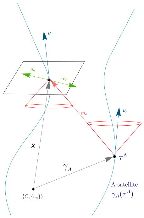
Figure 2.
User’s unit celestial sphere and inscribed tetrahedron defined by the relative positions of four emitters on it. Four inner tetrahedrons with common vertex on U and with a sole inscribed face on are also shown.
Figure 2.
User’s unit celestial sphere and inscribed tetrahedron defined by the relative positions of four emitters on it. Four inner tetrahedrons with common vertex on U and with a sole inscribed face on are also shown.
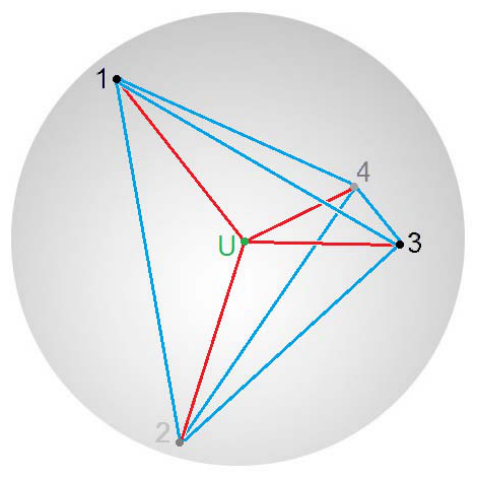

Table 1.
Computing the GDOP scalar from invariant quantities. Two highly symmetric configurations of four emitters are considered: a regular and an iso-rectangular tetrahedron.
Table 1.
Computing the GDOP scalar from invariant quantities. Two highly symmetric configurations of four emitters are considered: a regular and an iso-rectangular tetrahedron.
| Tetahedron | S | |||||||
|---|---|---|---|---|---|---|---|---|
| Regular | 64 | |||||||
| Iso-rectangular | 57 |
Disclaimer/Publisher’s Note: The statements, opinions and data contained in all publications are solely those of the individual author(s) and contributor(s) and not of MDPI and/or the editor(s). MDPI and/or the editor(s) disclaim responsibility for any injury to people or property resulting from any ideas, methods, instructions or products referred to in the content. |
© 2026 by the authors. Licensee MDPI, Basel, Switzerland. This article is an open access article distributed under the terms and conditions of the Creative Commons Attribution (CC BY) license (http://creativecommons.org/licenses/by/4.0/).
Copyright: This open access article is published under a Creative Commons CC BY 4.0 license, which permit the free download, distribution, and reuse, provided that the author and preprint are cited in any reuse.


